D2.5 Theoretic benchmark of key performance indicators (KPIs) · PDF fileTheoretic benchmark...

SANSA-645047 D2.5

D2.5

Theoretic benchmark of key performance indicators (KPIs)

Grant Agreement nº: 645047 Project Acronym: SANSA Project Title: Shared Access Terrestrial-Satellite Backhaul

Network enabled by Smart Antennas Contractual delivery date: 30/04/2016 Actual delivery date: 24/05/2016 Contributing WP 2 Dissemination level: Public Editors: Athens Information Technology (AIT) Contributors: Dimitrios Ntaikos (AIT), Kostas Ntougias (AIT),

Christos Tsinos (ULUX), George Agapiou (OTE)

Abstract: This deliverable contains the outcomes of Task 2.6. It includes the theoretical benchmark and upper bounds of the KPIs defined in Task 2.4.

D2.5: Theoretic benchmark of KPIs

Date: 30/04/2016

of 40

SANSA-645047 D2.5

Document History Version Date Editor Modification

0.1 01/02/2016 AIT Document creation with proposed Table of Contents and partners’ assignment

0.2 01/04/2016 AIT Modification of KPI’s 0.3 25/04/2016 AIT Integrated input from ULUX and OTE 0.4 26/04/2016 AIT Final additions, minor corrections, finalisation 0.5 11/05/2016 ΑΙΤ Addition of results for broadcast channel and multi-

hop relaying 0.6 – 0.9 11/05/2016

– 18/05/2016

AIT QA by AVA and TASE. Comments and proof reading by CTTC.

1.0 18/05/2016 AIT Final version


Date: 30/04/2016

of 40

SANSA-645047 D2.5

List of contributors Name Company Contributions include Dimitrios Ntaikos AIT Main editor; coordination and

integration of input by all partners. Contributor to Chapter 1, Chapter 2 (2.1), Chapter 3, Chapter 4.

Christos Tsinos ULUX Contributor to Chapter 2 (2.1.1 for the Helsinki Topology), Chapter 3.

George Agapiou OTE Executive Summary Kostas Ntougias AIT Chapter 1; Introduction to

Chapter 2; Section 2.1.2; Section 2.1.3; Contribution to Chapter 4.

George Ziaragkas AVA Proof reading; final quality assurance check

Isaak Moreno Asenjo TAS Proof reading; final quality assurance check

Kostas Voulgaris AIT Final editing


Date: 30/04/2016

of 40

SANSA-645047 D2.5

Table of Contents

List of Figures ...................................................................................................................................... 5

List of Tables ........................................................................................................................................ 6

List of Acronyms .................................................................................................................................. 7

Executive Summary ............................................................................................................................. 9

1 Introduction .............................................................................................................................. 10

2 Aggregated Throughput ............................................................................................................ 10

2.1 Parameters that affect aggregated throughput .................................................................... 10

2.1.1 Aggregated Throughput for the Helsinki Topology. .................................................. 12

2.1.2 Aggregated Throughput for Broadcast Channel Topology ....................................... 21

2.1.3 Aggregated Throughput for Multi-Hop Relaying Topology ....................................... 31

3 Energy efficiency ....................................................................................................................... 35

4 Conclusions ............................................................................................................................... 39

References ......................................................................................................................................... 40


Date: 30/04/2016

of 40

SANSA-645047 D2.5

List of Figures

Figure 2-1. Example Topology ........................................................................................................... 12 Figure 2-2. SINR distribution of the topology example ..................................................................... 14 Figure 2-3. The distribution of the required number of nulls with aggressive frequency reuse ........ 17 Figure 2-4. Aggregated Throughput with respect to SNR ................................................................. 19 Figure 2-5. Upper bound of the Aggregated Throughput with respect to the degrees of freedom per node ............................................................................................................................................ 21 Figure 2-6. Wireless terrestrial backhauling setups. ......................................................................... 22 Figure 2-7. SANSA demonstration setup. .......................................................................................... 23 Figure 2-8. System setup for 𝐾𝐾 = 2 and 𝐿𝐿 = 4................................................................................. 24 Figure 2-9 Numerical simulation results: Average SR throughput vs. low- and high-SNR capacity bounds. .............................................................................................................................................. 29 Figure 2-10 Numerical simulation results: average SR throughput of CIZF vs. ZF precoding. .......... 31 Figure 2-11 One-dimensional multi-hop network............................................................................. 32 Figure 2-12 Overall gain of directional antennas for 𝑎𝑎 = 2. ............................................................. 34 Figure 2-13 SIMO relay network. ...................................................................................................... 35 Figure 2-14 Example of achievable rate region in the case of omni-directional. ............................. 35 Figure 3-1. Energy Efficiency with respect to SNR ............................................................................ 37 Figure 3-2. Upper bound on the energy Efficiency with respect to the degrees of freedom per node ........................................................................................................................................................... 38


Date: 30/04/2016

of 40

SANSA-645047 D2.5

List of Tables

Table 2-1. Topology Parameters ....................................................................................................... 13 Table 2-2. Simulations Parameters ................................................................................................... 17 Table 2-3. Aggregated Throughput and Power requirements .......................................................... 18 Table 3-1. Energy Efficiency results for the topology example ......................................................... 36


Date: 30/04/2016

of 40

SANSA-645047 D2.5

List of Acronyms

AWGN Additive White Gaussian Noise BC Broadcast Channel

BER Bit Error Rate BLER Block Error Rate BPSK Binary Phase Shift Keying

BS Base Station CCI Co-Channel Interference CIZF Constructive Interference Zero Forcing CN Core Network CSI Channel State Information DL Downlink

DoF Degrees of Freedom DPC Dirty Paper Coding EE Energy Efficiency

FDD Frequency Division Duplex HPBM Half-Power Beam-width KPIs Key Performance Indicators

LC-PAA load-controlled parasitic antenna array LOS Line Of Sight LTE Long Term Evolution

MAMP multi-active multi-passive MRT Maximum Ration Transmission

MU-MISO Multi-User Multiple-Input Single Output PA Power Allocation

PSD Power Spectral Density PTMP Point-to-Multi-Point PTP Point to Point RAN Radio Access Network RF Radio Frequency Rx Receiver

RZF Regularised Zero-Forcing SER Symbol Error Rate

SGW Serving Gateway SIMO Single Input Multiple Output SINR Signal to Interference plus Noise Ratio


Date: 30/04/2016

of 40

SANSA-645047 D2.5

SISO Single Input Single Output SNR Signal to Noise Ratio SR Sum-Rate Tx Transmitter UL Uplink

ULA Uniform Linear Array WF Water Filling ZF Zero Forcing

ZMCSCG Zero-mean Circularly Symmetric Complex Gaussian


Date: 30/04/2016

of 40

SANSA-645047 D2.5

Executive Summary

This is Deliverable D2.5 of the SANSA project and contains the theoretic benchmark of the key performance indicators (KPIs). This deliverable is the outcome of Task 2.6.

The objective of this deliverable is to explicitly specify the theoretic benchmarks and upper bounds for the KPIs which are described in Task 2.4.

Firstly, the aggregated throughput of a terrestrial wireless backhaul system of a cellular mobile radio communication network is defined mathematically. It is the result of analysing the parameters that affect the aggregated throughput, which include the bandwidth, the SINR, and the number of hops. By determining the upper bounds on the above three parameters, results to the bound of the aggregated throughput are obtained.

In the next section, the power consumption of each backhaul node is defined. Its total value is the sum of the transmission power, the fixed load-independent circuit power and the power consumed due to signal processing operations. Thus, the Energy Efficiency is defined as the ratio of the Aggregate Throughput to the Power consumption. The parameters presented in this deliverable that affect the Energy efficiency include therefore the same parameters that affect the aggregated throughput; the bandwidth, the SINR, and the number of hops, as well as the energy consumed. The bounds on the above three parameters place a bound also on the energy efficiency.

Finally, in the conclusion section, a summary of the KPIs are presented with their effect to the improvement of the SANSA system.


Date: 30/04/2016

of 40

SANSA-645047 D2.5

1 Introduction

This document contains the outcome of Task 2.6. More specifically, it presents the theoretic benchmarks and upper bounds for the KPIs described in Task 2.4. Benchmarking is based on a conventional system which utilises currently available technologies and where satellite and terrestrial backhauling operate independently. The derivation of the upper bounds, in turn, is based on the determination of the factors that affect the corresponding KPIs as well as on the use of information-theoretic principles. These bounds represent the limit on the system’s performance. In scenarios of practical interest, the achieved performance will most likely be suboptimal due to several constraints (e.g., regarding cost, power consumption, and complexity) and non-idealities (e.g., transceiver impairments). Nevertheless, the calculation of these values will enable us to determine the gap of the proposed hybrid satellite-terrestrial mobile backhaul system and to evaluate its performance gains over conventional setups.

2 Aggregated Throughput

Consider a terrestrial wireless backhaul system of a cellular mobile radio communications network. The purpose of that system is to transfer traffic from the radio access network (RAN) to the core network (CN) and vice-versa. With the term “traffic”, we mean user data and control signalling associated with both uplink (UL) and downlink (DL) transmission. By backhaul we refer to the network of point-to-point (PTP) and point-to-multipoint (PTMP) links that convey the traffic between the Radio Access Network and the Core Network. For example, in the LTE terminology, this is network connecting the Serving Gateway (SGW) and the eNodeBs. Typically, the backhaul is built in a tree topology, with eNodeBs being located across the tree branches. Multihop is used to convey traffic from edge of the branches to those with dedicated links to the Core Network. In the SANSA architecture, however, the use of antenna arrays means that we each node may be able to use multiple routes to send its traffic to the core network. We define as aggregated throughput the data rate (in bits/s) available to each node as a result of its capability to use several links, simultaneously.

2.1 Parameters that affect aggregated throughput

The parameters that affect the aggregated throughput are:


Date: 30/04/2016

of 40

SANSA-645047 D2.5

• The available bandwidth at each link.

• The transmit power at each link.

• The distance between the transmitter (Tx) and receiver (Rx) at each link.

• The noise and interference levels.

• Path loss and fading.

• The topology.

• The number of hops in the end-to-end (i.e., source-destination) link.

More specifically, the throughput of the 𝑘𝑘-th link using bandwidth 𝐵𝐵𝑘𝑘 can be defined mathematically as

𝑅𝑅𝑘𝑘 = 𝐵𝐵𝑘𝑘 log2(1 + SINR𝑘𝑘), 𝑘𝑘 = 1,2, … ,𝐾𝐾 Eq. 1

where

SINR𝑘𝑘 = 𝑃𝑃𝑟𝑟,𝑘𝑘𝐼𝐼𝑘𝑘+𝑃𝑃𝑛𝑛,𝑘𝑘

Eq. 2

is the corresponding receive signal-to-interference-plus-noise-ratio (SINR), with 𝑃𝑃𝑟𝑟,𝑘𝑘 representing the receive power at the 𝑘𝑘-th RX, 𝐼𝐼𝑘𝑘 denoting the interference, and 𝑃𝑃𝑛𝑛,𝑘𝑘 referring to the additive noise at this Rx. The received power 𝑃𝑃𝑟𝑟,𝑘𝑘 depends on the transmitted power 𝑃𝑃𝑡𝑡,𝑘𝑘, the Tx – Rx separation, and the channel gain which in turn is determined by the path loss and fading. The interference that is present on the link depends on the topology and the transmit power of the surrounding intra- and inter-system nodes.

The aggregated throughput is expressed as:

𝑅𝑅 = ∑ 𝑅𝑅𝑘𝑘𝐾𝐾𝑘𝑘=1 = ∑ 𝐵𝐵𝑘𝑘log2(1 + SINR𝑘𝑘)𝐾𝐾

𝑘𝑘=1 Eq. 3

If the same bandwidth 𝐵𝐵 is available at all the links, the previous equation reduces to:

𝑅𝑅 = ∑ 𝑅𝑅𝑘𝑘𝐾𝐾𝑘𝑘=1 = 𝐵𝐵∑ log2(1 + SINR𝑘𝑘)𝐾𝐾

𝑘𝑘=1 Eq. 4


Date: 30/04/2016

of 40

SANSA-645047 D2.5

Note that the number of nodes 𝐾𝐾 that is required for transferring the traffic from the source to the destination depends on the topology and the routing mechanisms (e.g., the topology may offer various end-to-end routes and the routing mechanism may direct the traffic through the route with the minimum number of hops). The routing algorithm may also decide to transfer the traffic through multiple “parallel” routes, thus enhancing the aggregated throughput.

To summarise, we can express the previous list as follows:

• Bandwidth.

• SINR.

• Number of hops.

2.1.1 Aggregated Throughput for the Helsinki Topology.

Figure 2-1. Example Topology


Date: 30/04/2016

of 40

SANSA-645047 D2.5

In this section we will provide results regarding the aggregated throughput of the example topology that was firstly introduced in D2.3 [1] and here we re-describe it for the sake of completeness. The topology parameters are given in Table 2-1. Topology Parameters and the distribution of SINR per link is given in Figure 2-2, as it was derived by employing the ITU-R P.452-16 interference modeling [4], including the free space loss as well as the diffraction loss based on the Bullington model [2] to derive the SINR of each receiver.

Table 2-1. Topology Parameters

There we can see that all the receivers experience a SINR > 42dB, while a significant number of them experience a SINR > 60dB. This is to be expected, since the benchmark topology is the outcome of careful network planning through link registration by the national regulator.

This topology is comprised of a number of different links. Each link is established via a single input – single output channel with channel gain ℎ𝑖𝑖𝑖𝑖. We assume that there is a large line of sight path (specular path) of known magnitude and there are also a large number of independent paths. In this case a common channel model for SISO systems [3] is given by:


Date: 30/04/2016

of 40

SANSA-645047 D2.5

hij = � kk+1

𝜎𝜎ejθij + � 1k+1

𝒞𝒞𝒞𝒞(0,σ2) Eq. 5

where the first term is the specular path arriving with uniform phase θij and the second one is due to the aggregation of the large number of reflected and scattered paths, idepedent of θij. The parameter k is referenced as the so-called k-factor and it is the ratio of the energy in the specular path to the energy in the scattered paths; the larger k is, the more deterministic the channel becomes. The parameter 𝜎𝜎 denotes the total energy received from all the paths. The magnitude of such a variable is said to follow the so-called Rician Distribution [3]. 𝒞𝒞𝒞𝒞(0,σ2) denotes a circularly symmetric complex Gaussian random variable with zero mean and variance σ2.

Figure 2-2. SINR distribution of the topology example


Date: 30/04/2016

of 40

SANSA-645047 D2.5

This model is a good representative of the channel conditions, since backhaul links involve strong LOS paths followed by some paths through scattering which are captured by the second term of Eq. 5. The input – output relationship of a link from node i to node j is given by:

𝑦𝑦𝑖𝑖𝑖𝑖 = ℎ𝑖𝑖𝑖𝑖𝒙𝒙𝑖𝑖𝑖𝑖 + 𝑤𝑤𝑖𝑖𝑖𝑖 Eq. 6

where 𝑦𝑦𝑖𝑖𝑖𝑖 is the received signal at node j, 𝑤𝑤𝑖𝑖𝑖𝑖 is complex circular symmetric Gaussian noise of variance 𝜎𝜎𝑤𝑤2 , 𝑥𝑥𝑖𝑖𝑖𝑖 is which the transmitted signal from node i, which satisfies:

𝔼𝔼�|𝑥𝑥𝑖𝑖𝑖𝑖|2 � = 𝑃𝑃𝑖𝑖 Eq. 7

where 𝑃𝑃𝑖𝑖 is the transmit power of the i-th node. From an information theoretic point of view [3], the mutual information of each link is given by:

𝐶𝐶𝑖𝑖,𝑖𝑖 = 𝐵𝐵𝑖𝑖,𝑖𝑖𝑙𝑙𝑙𝑙𝑙𝑙2(1 + 𝑆𝑆𝐼𝐼𝑆𝑆𝑅𝑅𝑖𝑖𝑖𝑖�ℎ𝑖𝑖𝑖𝑖�2) Eq. 8

where the Signal-to-Interference-plus-noise Ratio (SINR) is defined as:

𝑆𝑆𝐼𝐼𝑆𝑆𝑅𝑅𝑖𝑖𝑖𝑖 = 𝑃𝑃𝑖𝑖𝜎𝜎𝑤𝑤2+𝐼𝐼𝑖𝑖𝑖𝑖

Eq. 9

and 𝐵𝐵𝑖𝑖,𝑖𝑖 is the bandwidth of the link.

The mutual information of a multi-hop Link 𝐿𝐿𝑘𝑘,𝑙𝑙 ⊂ [1,15] is known to be equal to [3]

𝐶𝐶𝑘𝑘,𝑙𝑙 = 𝑚𝑚𝑚𝑚𝑚𝑚(𝑖𝑖,𝑖𝑖)∈𝐿𝐿𝑘𝑘,𝑙𝑙

𝐶𝐶𝑖𝑖,𝑖𝑖 Eq. 10

Let us now assume that node 1 is the only source node that generated traffic in the topology. Furthermore, let us assume that nodes 2, 4, 5, 6, 7, 11, 12, 13, 14, 15 are the intended destinations of that traffic and the multi-hop paths via which the traffic is routed are:

𝐿𝐿1,2 = {(1,2)}

𝐿𝐿1,4 = {(1,4)}

𝐿𝐿1,5 = {(1,5)}


Date: 30/04/2016

of 40

SANSA-645047 D2.5

𝐿𝐿1,6 = {(1,6)}

𝐿𝐿1,7 = {(1,3), (3,7)}

𝐿𝐿1,11 = {(1,8), (8,10), (10,9), (9,11)}

𝐿𝐿1,12 = {(1,8), (8,10), (10,9), (9,12)}

𝐿𝐿1,13 = {(1,8), (8,10), (10,13)}

𝐿𝐿1,14 = {(1,8), (8,14)}

𝐿𝐿1,15 = {(1,8), (8,15)}

The network’s aggregated throughput is given by:

𝐶𝐶 = ∑ 𝐶𝐶𝑘𝑘,𝑙𝑙𝑘𝑘,𝑙𝑙 Eq. 11

The aim of this section is to derive some bounds regarding the aggregate throughput of the network of Figure 2-1 under different assumptions. For the low bound we consider the current condition of the topology where each link between the nodes has an allocated bandwidth of 56MHz, each node has only one antenna and no interference mitigation schemes are applied. Moreover, if two or more links involve the same node, e.g. 𝐿𝐿1,11 and 𝐿𝐿1,12 both pass through 8, 9 and 10, the total bandwidth is divided equally among them, for example via the round-robin technique.

Then, in order to calculate the upper bound, we assume full frequency reuse by each one of the nodes, and the interference between the links is mitigated completely by adequate techniques that involve multiple antennas at the nodes. Moreover, it is assumed that all the links can be accommodated simultaneously due to the multiple antennas in the nodes. The requirements for degrees of freedom are specified by the number of nulls that need to be placed in order to mitigate completely the interference and the number of simultaneous transmissions that the nodes must accommodate. The distribution of the number of nulls was derived in D2.3 and we summarize the result in Figure 2-3 for convenience. Based on this figure, we can deduce that each node needs to be able to produce 7 nulls in average. It is expected that if less aggressive frequency is used in combination with carrier allocation optimization, a smaller number of nulls will be required. Thus, this number can be considered as an upper bound requirement in SANSA smart antenna techniques.


Date: 30/04/2016

of 40

SANSA-645047 D2.5

Figure 2-3. The distribution of the required number of nulls with aggressive frequency reuse

The simulation parameters for both cases are summarized on Table 2-2. Table 2-3 depicts the results regarding the bounds on the capacity and the corresponding required transmission power to achieve them. Note that the required transmission power is computed by assuming that each transmitting node of a link (𝑚𝑚, 𝑗𝑗) ∈ 𝐿𝐿𝑘𝑘,𝑙𝑙 functions at a power such that the minimum capacity of the multi-hop link 𝐿𝐿𝑘𝑘,𝑙𝑙 is achieved (Eq.10).

Parameters Low Bound Upper Bound Maximum Power 38 dBW 38 dBW

Bandwidth per Link 56 MHz 784 MHz Table 2-2. Simulations Parameters


Date: 30/04/2016

of 40

SANSA-645047 D2.5

Parameters Low Bound Upper Bound Aggregated Throughput 5.3 ∗ 109 bits/sec 10.1 ∗ 1010 bits/sec

Power Requirements 47.8 dBW 47.8 dBW Table 2-3. Aggregated Throughput and Power requirements

As it is observed by the results of Table 2-3, by considering full frequency reuse and the availability of additional spatial degrees of freedom (multiple-antennas at the nodes), such that the interference is completely mitigated and all the links can be simultaneously accommodated, we may achieve throughput almost twenty times greater than the one of the current topology (low-bound).

The results of Table 2-3 are based on the reported SINR for the topology example. In Figure 2-4 we repeated the experiments for different mean SINR values in order to study the dependence of the aggregated throughput on the latter. As it can be seen, both the upper and the lower bounds are increasing with an increase in the SINR/SNR values.

Moreover, for the results concerning the Upper bound in the full frequency use scenario we assume that apart from the spatial degrees of freedom related to nulling and simultaneous transmission needs, each node has only one degree of freedom available for each one of the supported links. Thus the Upper bound can be further increased by adding additional degrees of freedom in each one of supported links. In this case the links are implemented via multi-antenna nodes and thus, the input-output relationship is now given by:

𝒚𝒚𝑖𝑖𝑖𝑖 = �𝑷𝑷𝑖𝑖𝑯𝑯𝑖𝑖𝑖𝑖𝒙𝒙𝑖𝑖𝑖𝑖 + 𝒘𝒘𝑖𝑖𝑖𝑖 Eq. 12

where 𝒚𝒚𝑖𝑖𝑖𝑖 is the 𝑅𝑅𝑥𝑥 × 1 received signal at node j, 𝒘𝒘𝑖𝑖𝑖𝑖 is complex circular symmetric 𝑅𝑅𝑥𝑥 × 1 vector Gaussian noise of covariance 𝜎𝜎𝑤𝑤2𝑰𝑰𝑅𝑅𝑥𝑥, 𝒙𝒙𝑖𝑖𝑖𝑖 is the 𝑇𝑇𝑥𝑥 × 1 transmitted signal from node i, which has the following covariance matrix:

𝑹𝑹𝑥𝑥 = 𝔼𝔼�𝒙𝒙𝑖𝑖𝑖𝑖𝒙𝒙𝑖𝑖𝑖𝑖𝐻𝐻� = 𝑷𝑷𝑖𝑖, Eq. 13

where 𝑷𝑷𝑖𝑖 is the power allocation matrix at the i-th node, 𝑇𝑇𝑥𝑥 is the number of transmit antennas, 𝑅𝑅𝑥𝑥 is the number of receive antennas and 𝑯𝑯𝑖𝑖𝑖𝑖 is the 𝑅𝑅𝑥𝑥 × 𝑇𝑇𝑥𝑥 matrix of the channel coefficients.


Date: 30/04/2016

of 40

SANSA-645047 D2.5

Figure 2-4. Aggregated Throughput with respect to SNR

It is easy to extend the previous model to the multi-antenna case. That is, the channel matrix between two nodes is now given by:

𝐇𝐇𝑖𝑖𝑖𝑖 = � kk+1

𝜎𝜎𝛼𝛼𝑖𝑖�𝜃𝜃𝑖𝑖�𝛼𝛼𝑖𝑖(𝜃𝜃𝑖𝑖)𝐻𝐻 +� 1k+1

𝒞𝒞𝒞𝒞(𝟎𝟎Rx×Tx ,𝜎𝜎2𝐈𝐈Rx×Tx) , Eq. 14

where

𝛼𝛼𝑖𝑖�𝜃𝜃𝑖𝑖� and 𝛼𝛼𝑖𝑖(𝜃𝜃𝑖𝑖)𝐻𝐻 are the responses of a (Uniform Linear Array) ULA which are given by:

𝛼𝛼𝑈𝑈𝐿𝐿𝑈𝑈(𝜃𝜃) + 1√𝛮𝛮

[1, 𝑒𝑒𝑖𝑖𝑗𝑗𝑗𝑗𝑗𝑗𝑖𝑖𝑛𝑛(𝜃𝜃), … , 𝑒𝑒𝑖𝑖(𝑁𝑁−1)𝑗𝑗𝑗𝑗𝑗𝑗𝑖𝑖𝑛𝑛(𝜃𝜃)], Eq. 15


Date: 30/04/2016

of 40

SANSA-645047 D2.5

where 𝑚𝑚 = 2𝜋𝜋𝜆𝜆

, d is the inter-element spacing, 𝑆𝑆 is the number of ULA’s elements, 𝟎𝟎Rx×Tx and 𝐈𝐈 Rx×Tx are the Rx × Tx matrix of zeros and identity matrix respectively and Rx , Tx are the number of receive and transmit antennas respectively. For more information, please refer to [3].

The mutual information of each link for the multi-antenna node case is given by:

𝐶𝐶𝑖𝑖,𝑖𝑖 = 𝐵𝐵 log2 |𝑰𝑰𝑅𝑅𝑥𝑥 + 1𝜎𝜎𝑤𝑤2𝑯𝑯𝑖𝑖𝑖𝑖𝑹𝑹𝑥𝑥𝑯𝑯𝑖𝑖𝑖𝑖

𝐻𝐻 |, Eq. 16

where B is the total available bandwidth and | ⋅ | is the determinant of the matrix. Now, it remains to compute the power allocation matrix 𝑷𝑷𝑖𝑖 which can be done by employing the so-called Water-Filling algorithm [3]. It can be shown that for high SNR values the WF solution converges to the equal power allocation one, that is:

𝑷𝑷𝑖𝑖 =

⎣⎢⎢⎡1𝑇𝑇𝑥𝑥

⋱1𝑇𝑇𝑥𝑥 ⎦⎥⎥⎤. Eq. 17

Note that the previous assumption is valid for backhaul networks since they are well-planned via high directional links as it can be also shown from the SINR values of Figure 2-2.

The upper bound on the aggregated throughput with respect to the number of available degrees of freedom per link is depicted in Figure 2-5, where it can be seen that additional spatial degrees of freedom provide better performance in terms of the aggregated throughput.


Date: 30/04/2016

of 40

SANSA-645047 D2.5

Figure 2-5. Upper bound of the Aggregated Throughput with respect to the degrees of freedom per node

2.1.2 Aggregated Throughput for Broadcast Channel Topology

Typically, the wireless terrestrial backhaul system in a mobile radio communications network consists of highly directional point-to-point links which connect each base station with a next-hop node through a narrow radiation beam, so that a (possibly multi-hop) route from each base station to the core network is established. To this end, the base stations are commonly equipped with microwave drum antennas.

However, in urban environments it is often difficult to follow this paradigm. This could be the case, for example, with small-cell base stations. An alternative to the conventional approach that suits


Date: 30/04/2016

of 40

SANSA-645047 D2.5

better this scenario is the use of multi-antenna nodes which utilize beamforming to connect with each other. In this case, the generated beams are not as narrow as the ones in the aforementioned method where drum antennas are employed. Therefore, precoding has to be used also on top of the beams in order to mitigate the resulting interference. Note that in this setup, the effect of scattering is much more prominent than in conventional highly directional point-to-point links, which are mainly characterized by their line-of-sight (LoS) component. Moreover, this method applies to any given radiation pattern, regardless of the utilized beam generation technique. However, due to the size, cost, and energy consumption constraints of small-cell radio access nodes, it is realistic to assume that a transceiver / antenna technology that utilizes a limited number of radio frequency (RF) chains and still provides a high number of degrees-of-freedom (DoF) is used. In addition, it makes sense to consider that a beam pattern is chosen among a set of fixed predetermined beams, so that the complexity is further reduced.

Having in mind the above, we consider the backhauling scenario that is depicted in Figure 2-6: a broadcast channel (BC) followed by a multi-hop relaying channel. The multi-antenna radio access node employs both beamforming (with “not-so-narrow” beams) and precoding to transmit over a broadcast channel to two other base stations, which then backhaul the data over a multi-hop relaying channel comprised by highly directional point-to-point links.

Figure 2-6. Wireless terrestrial backhauling setups.


Date: 30/04/2016

of 40

SANSA-645047 D2.5

The first-hop setup (i.e., the broadcast channel) is also consistent with the envisioned SANSA demo, as is illustrated in Figure 2-7. Hence, the study of the throughput bounds in this configuration is of great importance.

Figure 2-7. SANSA demonstration setup.

In this Section, we will study the performance bounds of the broadcast channel, while in the next one we will focus on the multi-hop relaying setup. Note that this work is highly generic and can be used with any radiation pattern and channel model.

System Setup

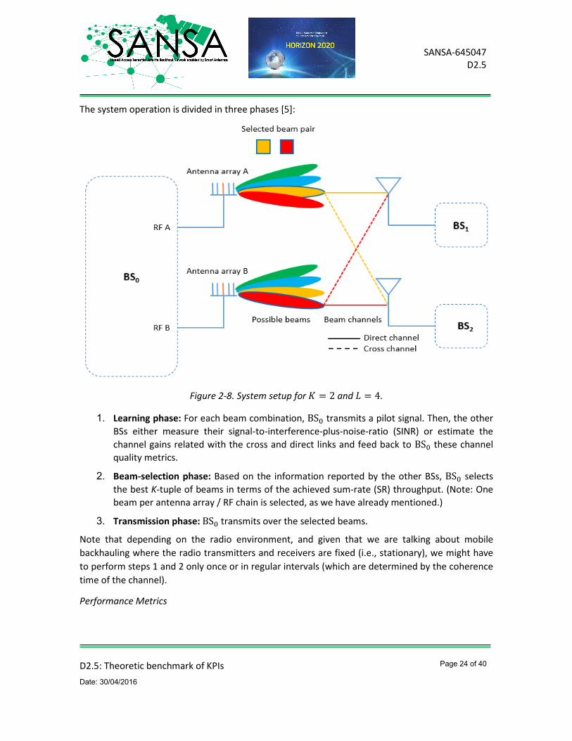
The transmitting base station (BS0) has 𝐾𝐾 (in general) RF chains / active antennas. In each time slot, it can generate 𝐾𝐾 beams (one per RF chain / active antenna). Each RF chain can choose one out of 𝐿𝐿 possible beams. This means that in each time slot, BS0 can choose 𝐾𝐾 out of 𝐿𝐿𝐾𝐾 possible beam combinations. Note that the number of antenna elements may be greater than the number of RF chains (e.g., this is the case when phased antenna arrays or parasitic antenna arrays are used). BS0 transmits data to 𝐾𝐾 other base stations (BS1 – BS𝐾𝐾) over a broadcast channel formed by the selected beams. Fig. 2-8 shows the system setup for 𝐾𝐾 = 2 and 𝐿𝐿 = 4.

Assumptions

We assume a flat- and block-fading channel model, a frequency division duplex (FDD) operating mode, and unit-variance additive noise. The receiving base stations utilize directional receive antennas.

Transmission Protocol


Date: 30/04/2016

of 40

SANSA-645047 D2.5

The system operation is divided in three phases [5]:

Figure 2-8. System setup for 𝐾𝐾 = 2 and 𝐿𝐿 = 4.

1. Learning phase: For each beam combination, BS0 transmits a pilot signal. Then, the other BSs either measure their signal-to-interference-plus-noise-ratio (SINR) or estimate the channel gains related with the cross and direct links and feed back to BS0 these channel quality metrics.

2. Beam-selection phase: Based on the information reported by the other BSs, BS0 selects the best K-tuple of beams in terms of the achieved sum-rate (SR) throughput. (Note: One beam per antenna array / RF chain is selected, as we have already mentioned.)

3. Transmission phase: BS0 transmits over the selected beams.

Note that depending on the radio environment, and given that we are talking about mobile backhauling where the radio transmitters and receivers are fixed (i.e., stationary), we might have to perform steps 1 and 2 only once or in regular intervals (which are determined by the coherence time of the channel).

Performance Metrics


Date: 30/04/2016

of 40

SANSA-645047 D2.5

Let’s assume that the beam combination (𝑙𝑙) has been selected. The data rate associated with the link formed between BS0 and BS𝑘𝑘, 𝑅𝑅𝑘𝑘 (𝑘𝑘 = 1,2, … ,𝐾𝐾), is given by

𝑅𝑅𝑘𝑘(𝑙𝑙) = log2 �1 + SINR𝑘𝑘

(𝑙𝑙)�, Eq. 18

and the SR throughput is expressed as

𝑅𝑅(𝑙𝑙) = ∑ 𝑅𝑅𝑘𝑘(𝑙𝑙)𝐾𝐾

𝑘𝑘=1 = ∑ log2 �1 + SINR𝑘𝑘(𝑙𝑙)�𝐾𝐾

𝑘𝑘=1 . Eq. 19

Channel Quality Metrics

During the learning phase, BS𝑘𝑘 (𝑘𝑘 = 1,2, … ,𝐾𝐾) can report back to BS0 its SINR for each beam combination 𝑙𝑙 = 1,2, … , 𝐿𝐿𝐾𝐾:

SINR𝑘𝑘(𝑙𝑙) =

�ℎ𝑘𝑘0(𝑙𝑙)�

2𝑝𝑝𝑘𝑘

∑ �ℎ𝑚𝑚0(𝑙𝑙) �

2𝑝𝑝𝑚𝑚𝑚𝑚≠𝑘𝑘 +1

. Eq. 20

In Eq. 20, ℎ𝑘𝑘0(𝑙𝑙) ∈ ℂ is the channel for the given beam combination (𝑙𝑙) between BS0 and BS𝑘𝑘, 𝑝𝑝𝑘𝑘 =

𝑝𝑝𝑗𝑗 = 1𝐾𝐾𝑃𝑃 is the transmission power of each link (i.e., during the learning phase it is applied

uniform power allocation), and 𝑃𝑃 is the total transmission power.

Alternatively, BS𝑘𝑘 may report to BS0 the direct channel ℎ𝑘𝑘0(𝑙𝑙) and the cross channels ℎ𝑘𝑘0,𝑗𝑗

(𝑙𝑙) (see Figure 2-8) for each beam combination (𝑙𝑙) – that is, they may feed channel state information (CSI)

back to BS0. Then, BS0 compiles the composite channel matrix 𝐇𝐇(𝑙𝑙) = �𝐡𝐡1(𝑙𝑙) 𝐡𝐡2

(𝑙𝑙) ⋯ 𝐡𝐡𝐾𝐾(𝑙𝑙)�

†∈

ℂ𝐾𝐾×𝐾𝐾, where 𝐡𝐡𝑘𝑘(𝑙𝑙) = �ℎ𝑘𝑘0

(𝑙𝑙) ℎ𝑘𝑘0,1(𝑙𝑙) ⋯ ℎ𝑘𝑘0,𝐾𝐾

(𝑙𝑙) �𝑇𝑇∈ ℂ𝐾𝐾×1 is the vector that holds the direct and

cross channels between BS0 and BS𝑘𝑘.

Beam Selection Criteria

After switching through all possible beam combinations, BS0 selects the optimum beam combination according to one of the following rules, depending on the type of channel quality metric reported back by the other BSs:

• SINR-based beam selection criterion: The 𝐾𝐾-tuple of beams (𝑙𝑙) that results in the maximum SR throughput 𝑅𝑅(𝑙𝑙) (see Eq. 19) is selected.

• CSI-based beam selection criterion: The 𝐾𝐾-tuple of beams (𝑙𝑙) that results in the minimum

value of the metric 𝑇𝑇(𝑙𝑙) = tr ��𝐇𝐇(𝑙𝑙)�𝐇𝐇(𝑙𝑙)�†�−1� is selected.

System Model


Date: 30/04/2016

of 40

SANSA-645047 D2.5

After beam selection, transmission takes place. The system model can be expressed as

𝐲𝐲 = 𝐇𝐇𝐇𝐇 + 𝐧𝐧, Eq. 21

where 𝐲𝐲 = [𝑦𝑦1 𝑦𝑦2 ⋯ 𝑦𝑦𝐾𝐾]𝑇𝑇 ∈ ℂ𝐾𝐾×1 is the vector of received symbols with 𝑦𝑦𝑘𝑘 ∈ ℂ being the symbol received at BS𝑘𝑘; 𝐧𝐧 = [𝑚𝑚1 𝑚𝑚2 ⋯ 𝑚𝑚𝐾𝐾]𝑇𝑇 ∈ ℂ𝐾𝐾×1 is the zero-mean circularly symmetric complex Gaussian (ZMCSCG) additive noise vector with unit variance, i.e., 𝐧𝐧~𝒞𝒞𝒞𝒞(𝟎𝟎𝐾𝐾 , 𝐈𝐈𝐾𝐾), with 𝑚𝑚𝑘𝑘~𝒞𝒞𝒞𝒞(0,1); and 𝐇𝐇 ∈ ℂ𝐾𝐾×𝐾𝐾 is the composite channel matrix. (Note that, for notational convenience, we have omitted the beam combination index as well as the dependence of the received signal on the path loss and shadowing effects. The latter is assumed that are absorbed in the variance of the composite channel matrix elements.)

If no precoding takes place, then 𝐇𝐇 = �𝐏𝐏1 2⁄ 𝐬𝐬� ∈ ℂ𝐾𝐾×1 and Eq. 21 becomes

𝐲𝐲 = 𝐇𝐇𝐏𝐏1 2⁄ 𝐬𝐬 + 𝐧𝐧, Eq. 22

where 𝐬𝐬 = [𝑠𝑠1 𝑠𝑠2 ⋯ 𝑠𝑠𝐾𝐾]𝑇𝑇 ∈ ℂ𝐾𝐾×1 is the transmitted symbols vector with 𝑠𝑠𝑘𝑘 ∈ ℂ being the symbol transmitted to BS𝑘𝑘 and 𝑃𝑃 = diag��𝑝𝑝1,�𝑝𝑝2, … ,�𝑝𝑝𝐾𝐾� is the power allocation (PA) matrix.

If precoding is utilized, on the other hand, then 𝐇𝐇 = �𝐖𝐖𝐏𝐏1 2⁄ 𝐬𝐬� ∈ ℂ𝐾𝐾×1 and Eq. 21 becomes

𝐲𝐲 = 𝐇𝐇𝐖𝐖𝐏𝐏1 2⁄ 𝐬𝐬 + 𝐧𝐧, Eq. 23

where 𝐖𝐖 = [𝐰𝐰1 𝐰𝐰2 ⋯ 𝐰𝐰𝐾𝐾] ∈ ℂ𝐾𝐾×𝐾𝐾 is the precoding matrix and 𝐰𝐰𝑘𝑘 ∈ ℂ𝐾𝐾×1 is the beamforming vector used to transmit 𝑠𝑠𝑘𝑘 to BS𝑘𝑘. In this case, the SINR at BS𝑘𝑘 is given by

SINR𝑘𝑘 =�𝐡𝐡𝑘𝑘†𝐰𝐰𝑘𝑘�

2𝑝𝑝𝑘𝑘

∑ �𝐡𝐡𝑘𝑘†𝐰𝐰𝑚𝑚�

2𝑝𝑝𝑚𝑚𝑚𝑚≠𝑘𝑘 +1

. Eq. 24

Multi-Cell Precoding

We consider three precoding variants. In maximum ratio transmission (MRT), the beamforming vectors are matched to the intended destination’s channel vector, as we can see in Eq. 25:

𝐯𝐯𝑘𝑘(MRT) = 𝐡𝐡𝒌𝒌 Eq. 25a

𝐰𝐰𝑘𝑘(MRT) = 𝐯𝐯𝑘𝑘

(MRT)

�𝐯𝐯𝑘𝑘(MRT)�

Eq. 25b

Note that the beamforming vector is normalized, as it is the standard practice.

In zero-forcing (ZF) precoding, the beamforming vectors are orthogonal to the subspace of non-intended receivers vectors, so that the co-channel interference (CCI) is nulled, i.e.,


Date: 30/04/2016

of 40

SANSA-645047 D2.5

�𝐡𝐡𝑘𝑘†𝐰𝐰𝑗𝑗

(ZF)�𝟐𝟐

= 0. Eq. 26

The ZF condition is translated into the use of the Moore-Penrose pseudo-inverse of the composite channel matrix as the precoding matrix:

𝐅𝐅(ZF) = 𝐇𝐇+ = 𝐇𝐇†�𝐇𝐇𝐇𝐇†�−𝟏𝟏 Eq. 27a

𝐖𝐖(ZF) = 𝐅𝐅(ZF)(:,𝑘𝑘)�𝐅𝐅(ZF)(:,𝑘𝑘)�

Eq. 27b

In this case, the SINR at BS𝑘𝑘 is given by

SINR𝑘𝑘 = �𝐡𝐡𝑘𝑘†𝐰𝐰𝑘𝑘

(ZF)�𝑝𝑝𝑘𝑘 . Eq. 28

Finally, in regularized zero-forcing (RZF) precoding, the ZF precoding matrix is regularized:

𝐅𝐅(RZF) = 𝐇𝐇† �𝐈𝐈𝐾𝐾 + 𝑃𝑃𝐾𝐾𝐇𝐇𝐇𝐇†�

−𝟏𝟏 Eq. 29a

𝐖𝐖(RZF) = 𝐅𝐅(RZF)(:,𝑘𝑘)�𝐅𝐅(RZF)(:,𝑘𝑘)�

Eq. 29b

The parameter 𝜆𝜆 = 𝑃𝑃 𝐾𝐾⁄ has been chosen so that the SINR at each receiver is maximized.

Power Allocation

In order to find the power allocation scheme that we will utilize in this setup, we have to solve the optimization problem

max𝐏𝐏≥0

∑ log2(1 + SINR𝑘𝑘)𝐾𝐾𝑘𝑘=1

s. t. ∑ ‖𝒘𝒘𝑘𝑘‖2𝐾𝐾𝑘𝑘=1 ≤ 𝑃𝑃

Eq. 30

This problem results in a water-filling solution.

Sum-Rate Capacity Bounds vs. SNR

In the high signal-to-noise-ratio (SNR) regime, the BC capacity is given by

limSNR→∞

𝐶𝐶BC ≈ 𝐾𝐾 log2 SNR . Eq. 31

In the low SNR regime, on the other hand, the optimum transmission strategy is to schedule only a receiving BS at each time slot. Then, the multi-user multiple-input single-output (MU-MISO) capacity is given by


Date: 30/04/2016

of 40

SANSA-645047 D2.5

limSNR→0

𝐶𝐶BC ≈ SNR log2 𝑒𝑒 . Eq. 32

Note: Please notice that the Shannon’s “log2” expression for the sum-rate throughput given in Eq. 19 represents already a performance bound for the transmission techniques of interest presented in a previous paragraph, since it assumes an infinite-length Gaussian input, which can be attained (or at least approached) by using appropriate modulation and coding schemes. The optimum transmission strategy is dirty paper coding (DPC), but this non-linear multi-user encoding scheme is seldom used in practice due to its high complexity. ZF precoding approaches the BC capacity in the DoF-limited high SNR regime, especially when the number of receivers is large, but it is highly suboptimal in the power-limited low SNR regime due to its power inefficiency. MRT, on the other hand, is optimum in the low SNR regime, since in this case the beamforming gain is translated into a linear capacity gain, but its capacity floors in the high SNR regime, since it cannot handle the CCI. RZF approaches the performance of ZF and MRT in the high and low SNR regimes, respectively, and performs significantly better in intermediate SNR values.

Sum-Rate Capacity Bounds vs. SNR for Setups Utilizing Parasitic Antenna Arrays

Let us consider the case where BS0 makes use of a multi-active multi-passive (MAMP) antenna array, comprised of 𝐾𝐾 active elements and 𝛫𝛫(𝛭𝛭− 1) passive elements which are connected to loads with purely imaginary impedance. Then, there is an additional beamforming gain of 𝑀𝑀 2⁄ associated with each link, in comparison with the case where a conventional antenna array is utilized. Therefore, the high-SNR and low-SNR regime SR-capacity bounds become [6]

limSNR→∞

𝐶𝐶BC ≈ 𝐾𝐾 log2 �𝑀𝑀2

SNR� . Eq. 33

limSNR→0

𝐶𝐶BC ≈ SNR𝑀𝑀2

log2 𝑒𝑒 . Eq. 34

Performance Evaluation

In this paragraph, we evaluate the performance of the considered system setup for the use case that is depicted in Figure 2-8 through numerical simulations over target receive SNR values in the range [−20,30]dB. We assume that BS0 utilizes a MAMP with 𝐾𝐾 = 2 and 𝑀𝑀 = 5. We consider (a) transmission without precoding, where the beam pair selection is based on SINR feedback; (b) ZF precoding transmission, where the beam pair selection is based on SINR feedback; (c) MRT, ZF, and RZF precoding transmission where the beam pair selection is based on CSI feedback; and (d) ZF precoding transmission in an equivalent, in terms of the number of RF chains, setup where BS0 is equipped with a conventional antenna array instead of a load-controlled parasitic antenna array (LC-PAA). The performance results represent ergodic SR throughput obtained after 1,000 simulation runs by taking the expectation of the corresponding SR equations. A single-bounce


Date: 30/04/2016

of 40

SANSA-645047 D2.5

scattering model has been incorporated in the simulations to capture both the effects of beamforming-based transmission as well as of small-scale and large-scale fading. The beams have been calculated with the help of appropriate antenna design software. They have a half-power beam width (HPBM) of 30∘.

The simulation results are illustrated in Figure 2-9. For comparison purposes, we have plotted also the high-SNR and low-SNR SR-capacity bounds for the considered setup, which are given by Eq. 33 and Eq. 34, respectively. As can be seen, at high SNR, a 5-fold sum rate gain is attained when using ZF precoding and beam selection as opposed to non-precoded beam selection, showing the importance of precoding in such setups.

Figure 2-9 Numerical simulation results: Average SR throughput vs. low- and high-SNR capacity bounds.

More specifically, a number of other interesting remarks can be made based on Figure 2-9.

• The average SR throughput of non-precoding-based transmission and MRT floors at high SNR due to the residual CCI, as expected.

• ZF precoding with LC-PAA outperforms its conventional antenna array counterpart over the entire SNR range, even when the beam pair selection is based on SINR feedback, due to the power gain attributed to transmit beamforming.

• Beam pair selection based on CSI feedback improves significantly the performance of ZF precoding, since in this case the beam pair selection and precoding tasks are performed jointly.


Date: 30/04/2016

of 40

SANSA-645047 D2.5

• Non-precoding-based transmission outperforms ZF precoding with conventional antenna array over the entire range of relevant SNRs (i.e., until the SR throughput flooring at the high SNR regime occurs). In fact, non-precoding-based transmission almost resembles MRT. Hence, we note that we can significantly reduce complexity and still pay only a negligible penalty on performance.

• We note that MRT is optimal at low SNR, ZF with beam pair selection based on CSI feedback is optimal at high SNR, and RZF approaches these two extremes at the corresponding SNR regimes while it performs better at intermediate SNRs, as expected.

• Finally, we notice that we achieve about 10dB worse performance than the high-SNR SR-capacity bound.

Constructive Interference Zero-Forcing Precoding

Conventional node-level linear precoding methods aim to reduce or even eliminate CCI. However, in some cases CCI may be constructive, in terms of the received SNR, instead of destructive at symbol-level. Constructive interference zero-forcing (CIZF) precoding is a symbol-level precoding scheme that “zero-forces” only the destructive interference, while leaving the constructive interference (CI) unaffected.

The precoding matrix is expressed as [7]

𝐖𝐖(CIZF) = 𝐖𝐖(ZF)𝐓𝐓 = 𝐇𝐇†𝐑𝐑−𝟏𝟏𝐓𝐓, Eq. 35

where

𝐑𝐑 = 𝐇𝐇𝐇𝐇†. Eq. 36

The matrix 𝐓𝐓 is calculated in a symbol-by-symbol basis as follows: First, 𝐑𝐑 is calculated according to Eq. 36. Then, 𝐆𝐆 ∈ ℂ𝐾𝐾×𝐾𝐾 is calculated. Assuming Binary Phase Shift Keying (BPSK) modulation (i.e., 𝑠𝑠𝑘𝑘 = ±1, 𝑘𝑘 = 1,2, … ,𝐾𝐾), we have

𝐆𝐆 = diag(𝐬𝐬)Re(𝐑𝐑) diag(𝐬𝐬). Eq. 37

Then, 𝜏𝜏𝑘𝑘𝑘𝑘 = 𝜌𝜌𝑘𝑘𝑘𝑘 and 𝜏𝜏𝑘𝑘𝑗𝑗 = 0 if 𝑙𝑙𝑘𝑘𝑗𝑗 < 0 or 𝜏𝜏𝑘𝑘𝑗𝑗 = 𝜌𝜌𝑘𝑘𝑗𝑗 otherwise, where

𝜌𝜌𝑘𝑘𝑗𝑗 = 𝐡𝐡𝑘𝑘𝐡𝐡𝑚𝑚†

‖𝐡𝐡𝑘𝑘‖‖𝐡𝐡𝑚𝑚‖ Eq. 38

is the 𝑘𝑘,𝑚𝑚-th element of 𝐑𝐑 and represents the cross-correlation factor between the channel vector of BS𝑘𝑘 and the mth transmitted data stream.

The SINR at BS𝑘𝑘 is given by

SINR𝑘𝑘 = ∑ |𝜏𝜏𝑘𝑘𝑗𝑗|2𝐾𝐾𝑗𝑗=1 𝑝𝑝𝑗𝑗. Eq. 39


Date: 30/04/2016

of 40

SANSA-645047 D2.5

The power-allocation problem for maximizing the SR-throughput under a sum-power constraint is solved using the water-filling algorithm, as in the node-level linear precoding scenario.

However, in this case the Shannon’s “log2” SR-throughput formulas are not useful as performance metrics, due to the strong dependence of CIZF from the utilized modulation scheme. Hence, we use instead the following formula:

𝑅𝑅 = (1 − BLER)𝑚𝑚, Eq. 40

where 𝑚𝑚 = 1 bit/symbol for BPSK and the block error rate (BLER) is given by

BLER = 1 − (1 − 𝑃𝑃𝑒𝑒)𝑁𝑁𝑓𝑓 , Eq. 41

with 𝑃𝑃𝑒𝑒 being the symbol / bit error rate (SER/BER) for BPSK and 𝑆𝑆𝑓𝑓 being the frame size.

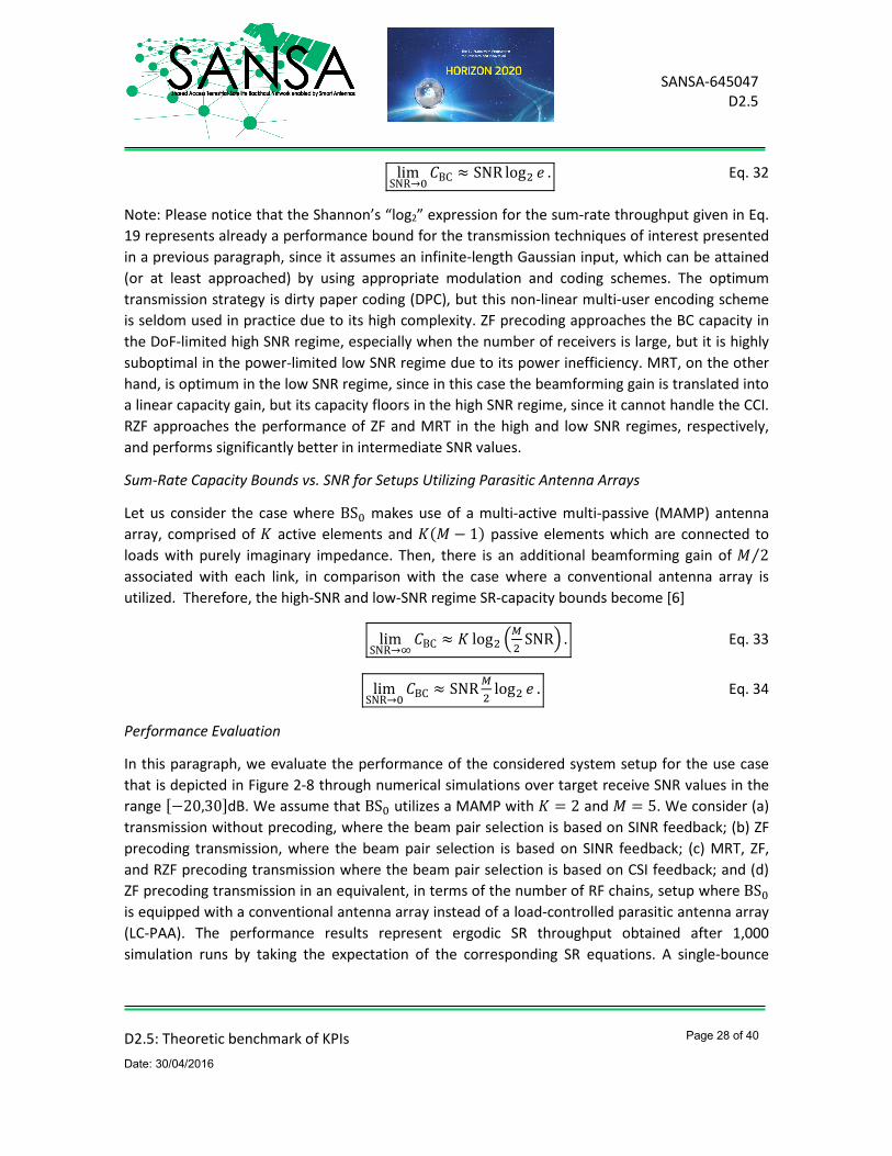
Figure 2-10 shows the SR throughput performance of ZF with CSI-based beam pair selection and CIZF precoding schemes for BPSK input signals and frame size 𝑆𝑆𝑓𝑓 = 100. We note that CIZF outperforms ZF precoding. A performance gain of about 7dB is observed. This gain is reduced with SNR. From SNR = 20dB and onwards, these precoding methods perform identical.

Figure 2-10 Numerical simulation results: average SR throughput of CIZF vs. ZF precoding.

2.1.3 Aggregated Throughput for Multi-Hop Relaying Topology

A terrestrial wireless mobile backhaul system is typically modelled as a multi-hop relaying channel where the nodes utilize directional antennas. It is of special importance to examine and evaluate


Date: 30/04/2016

of 40

SANSA-645047 D2.5

the advantages of employing directional antennas in such a setup against omni-directional antennas. In the following, we assume setups with directional relay nodes and no scattering, as it is suitable for conventional microwave line-of-sight (LoS) relaying.

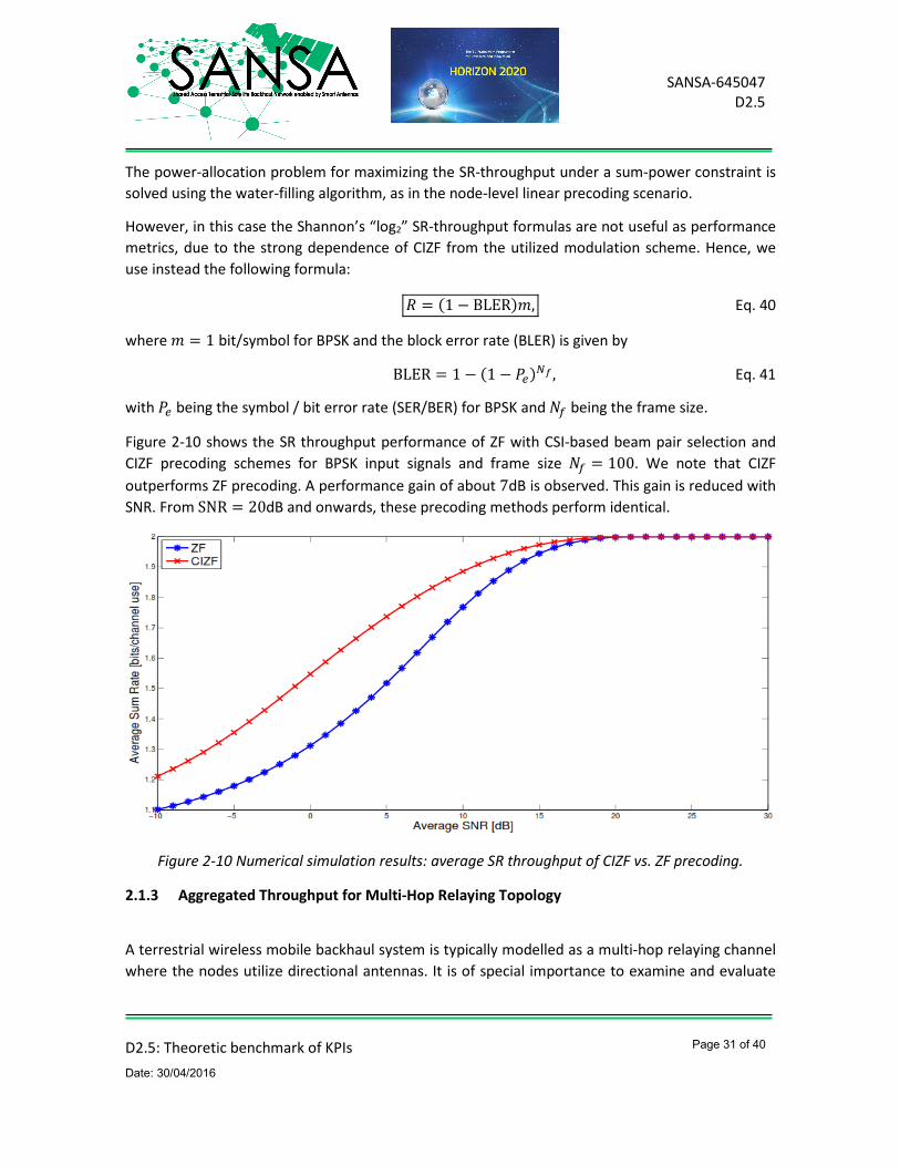
Initially, as Figure 2-11 shows, we consider a one-dimensional system with a single source node S, a single destination node D, and 𝑆𝑆 − 1 intermediate nodes F𝑖𝑖, 𝑚𝑚 = 1,2, … ,𝑆𝑆 − 1, which act as relays, are placed at equal intervals in a distance 𝐿𝐿 = 1, and share a band of radio frequencies allowing for a signalling rate of 𝑊𝑊 complex-valued symbols per second.

Figure 2-11 One-dimensional multi-hop network.

The goal is to deliver packets that are generated at the source S at a (bandwidth-normalized) rate of 𝑅𝑅 bits per second per Hertz to the destination node reliably, using coded transmission and consuming the least possible transmission power 𝑃𝑃𝑇𝑇. We assume that this power is equally allocated among the transmitting nodes. We also assume ideal directional antennas (i.e., without back- and side-lobes) with high gain and directivity. Also, we assume half-duplex decode-and-forward operation and additive white Gaussian noise (AWGN) with power spectral density (PSD) 𝑆𝑆0 2⁄ . Interference from all nodes transmitting simultaneously with the preceding node is regarded as additional Gaussian noise. The signal from node to node experiences path loss with exponent 𝛼𝛼. The attenuation factor is given by

𝛼𝛼𝑗𝑗,𝑖𝑖 = 𝑑𝑑(𝑠𝑠, 𝑚𝑚)−𝛼𝛼, Eq. 42

where 𝑑𝑑(𝑠𝑠, 𝑚𝑚) is the distance between the nodes. The path loss exponent 𝛼𝛼 typically takes values between 2 and 4.

To facilitate parallel transmission of several packets through the network, the available bandwidth is reused between transmitters, with a minimum separation of 𝐾𝐾 hops between simultaneously transmitting nodes (2 ≤ 𝐾𝐾 ≤ 𝑆𝑆). The achievable end-to-end rate is based on the minimum of the rates achieved at each hop.


Date: 30/04/2016

of 40

SANSA-645047 D2.5

For the case of omni-directional antennas, the bandwidth-normalized rate was quantified in [8] and is given by the following equation:

𝑅𝑅 = min𝑖𝑖=0,…,𝑁𝑁−1

�1𝐾𝐾

log2 �1 + 𝑃𝑃𝑖𝑖𝑁𝑁𝛼𝛼

𝑊𝑊𝑁𝑁0+∑ 𝑃𝑃𝑆𝑆(𝑅𝑅)𝑆𝑆∈𝑆𝑆𝑖𝑖 |𝑖𝑖+1−𝑗𝑗|−𝛼𝛼�� , Eq. 43

where 𝑃𝑃𝑖𝑖 = 𝐾𝐾𝑁𝑁𝑃𝑃𝑇𝑇 is the transmit power of each relay node and 𝑆𝑆𝑖𝑖 is the set of nodes that are

transmitting simultaneously with node F𝑖𝑖, i.e.,

𝑆𝑆𝑖𝑖 = {𝑠𝑠 ∈ {0,1, … ,𝑆𝑆 − 1}|𝑠𝑠 ≠ 1 and 𝐾𝐾 divides 𝑚𝑚 − 𝑠𝑠}. Eq. 44

The energy per bit to noise spectral density is given by

𝐸𝐸𝑏𝑏∗(𝑅𝑅)𝑁𝑁0

= �2𝐾𝐾𝐾𝐾−1�𝐾𝐾−1𝑁𝑁−𝑎𝑎

𝑅𝑅𝛽𝛽𝑖𝑖(𝑅𝑅)−(2𝐾𝐾𝐾𝐾−1)𝑅𝑅∑ 𝛽𝛽𝑆𝑆(𝑅𝑅)𝑆𝑆∈𝑆𝑆𝑖𝑖 |𝑖𝑖+1−𝑗𝑗|−𝛼𝛼, Eq. 45

where 𝑅𝑅 is the achievable rate, 𝐸𝐸𝑏𝑏∗ is the sum of energies per bit spent over all hops, and 𝛽𝛽𝑖𝑖(𝑅𝑅) are all functions of 𝑅𝑅 that satisfy

∑𝛽𝛽𝑖𝑖(𝑅𝑅) = 1. Eq. 46

In the case of directional antennas, each node receives interference only from the currently active preceding ones:

𝑆𝑆𝑖𝑖 = {𝑠𝑠 ∈ {0,1, … ,𝑆𝑆 − 1}|𝑠𝑠 < 1 and 𝐾𝐾 divides 𝑚𝑚 − 𝑠𝑠}. Eq. 47

Three benefits arise from the use of directional antennas and affect positively the achieved spectral efficiency [9]:

• Power gain: The minimum required transmission power and the beam width of the antenna are proportional to each other. That is, if we use an ideal directional antenna with half the angle of transmission, then we will also have to transmit with half the power (assuming LoS propagation). Hence, if we use, for example, beams of 60∘, the transmitted power is reduced by 6 times (~8 dB) in comparison with the omni-directional antennas case.

• Reuse factor gain: Directional antennas affect also the “spatial reuse factor.” In the case of omni-directional antennas, it was shown in [8] that the optimal number of hops that should separate the simultaneous transmitting nodes is 𝐾𝐾 = 3, while in [9] it was shown that for the case of directional antennas it is 𝐾𝐾 = 2. Thus, directional antennas allow for denser networks and more parallel transmission channels.

• Interference gain: Another advantage of directional antennas is that each node receives interference only from the preceding active ones.


Date: 30/04/2016

of 40

SANSA-645047 D2.5

Figure 2-12 shows the overall gain associated with the use of directional antennas for various values of 𝑆𝑆 and 𝐾𝐾 and for 𝛼𝛼 = 2, assuming a constant total power in the network. The numerical simulation results indicate that 60 ∘ directional antennas provide a 3-fold gain of the achievable rate.

Figure 2-12 Overall gain of directional antennas for 𝑎𝑎 = 2.

In [10] the achievable rate region of a two-dimensional single-input multiple-output (SIMO) relay network was studied (see Figure 2-13).


Date: 30/04/2016

of 40

SANSA-645047 D2.5

Figure 2-13 SIMO relay network.

It was shown that the use of directional antennas can improve the sum-rate up to 6 times in comparison with the omni-directional antennas case, as it is illustrated in Figure 2-14.

Figure 2-14 Example of achievable rate region in the case of omni-directional.

These works can serve as a baseline for deriving SR-capacity results for the SANSA topology with arbitrary beam patterns and scattering.

3 Energy efficiency

The energy efficiency (EE) of a link is defined as:

𝐸𝐸𝐸𝐸[bit/Joule] =Aggregate Throughput� bit

channel use�

Power Consumption� Joulechannel use�

Eq. 48


Date: 30/04/2016

of 40

SANSA-645047 D2.5

The power consumption of each backhaul node is divided in three parts, one referring to the transmission power, another representing fixed load-independent circuit power (e.g., required for filters, mixers etc.), and yet another one related with the power consumed due to signal processing operations.

For the Helsinki topology the results regarding the energy efficiency is depicted in Table 3-1. Here, as power consumption we consider only the transmission one since we do not have information related to the actual equipment in the base stations of the topology.

Parameters Low Bound Upper Bound Energy Efficiency 8.7 ∗ 104 bits/Joule 1.7 ∗ 106 bits/Joule

Table 3-1. Energy Efficiency results for the topology example

Furthermore, in Figure 3-1 and Figure 3-2 we depict the energy efficiency with respect the SNR values and the additional degrees of freedom similar to the case of the aggregated throughput of 2.1.1. We can also see that the energy efficiency increases with the SNR value and the additional degrees of freedom.


Date: 30/04/2016

of 40

SANSA-645047 D2.5

Figure 3-1. Energy Efficiency with respect to SNR


Date: 30/04/2016

of 40

SANSA-645047 D2.5

Figure 3-2. Upper bound on the energy Efficiency with respect to the degrees of freedom per node


Date: 30/04/2016

of 40

SANSA-645047 D2.5

4 Conclusions In this Deliverable, D2.5, we defined the aggregated throughput of a terrestrial wireless backhaul system of a cellular mobile radio communication network.

In the Helsinki topology, the lower bound for the aggregated throughput per link was found to be 5.3*109 bits/sec, while the upper bound was 10.1*1010 bits/sec, assuming a maximum power per antenna of the order of 47.8 dBW so that the minimum capacity of the multi-hop link is achieved.

Also, in a broadcast channel topology that is suitable for the terrestrial segment in medium-to-rich scattering environments, we presented sum rate bounds for transmission methods that employ arbitrary beam patterns and low cost / low power consumption transceivers. The bounds indicate that the combination of simple precoding and beam selection can provide a 5-fold gain in sum rate capacity for 2-branch broadcast channel configurations that employ transmission antennas of 30 degree half-power beam width.

Furthermore, in a multi-hop relaying topology, suitable for terrestrial segments with Line-of-Sight / low scattering propagation conditions and highly directive antennas, we investigated the performance gains, in terms of the achieved sum-rate throughput, of setups that utilize directional antennas over configurations that make use of omni-directional antennas. The numerical simulations’ results indicate that directional antennas of 8dB gain in the direction of transmission can provide up to a 6-fold end-to-end capacity increase over omni-antenna relaying with the same number of hops. The understanding of the effect of the beam width / directionality in the overall spectral efficiency will be useful in evaluating the performance of the SANSA system for given beam patterns.

Moreover, we defined the energy efficiency of a link as the aggregated throughput over the power consumption. The latter consists of the transmitted (over-the-air) power, the power consumed inside the circuitry (e.g. filters, mixers etc.) and the power spent for the signal processing. In the topology we examined in Helsinki, the energy efficiency in terms of transmitted power was found to be of the order of 8.7*104 bits/Joule as per the lower bound and 1.7*106 bits/Joule for the upper bound.

Both the aggregated throughput and the energy efficiency increase with the SNR value.


Date: 30/04/2016

of 40

SANSA-645047 D2.5

References [1] D2.3 “Definition of reference scenarios, overall system architectures, research challenges,

requirements and KPIs” from SANSA project.

[2] Abdollah Ghasemi, Ali Abedi, Farshid Ghasemi, “Propagation Engineering in Wireless Communications”, Chapter 6, Springer.

[3] Tse, David, and Pramod Viswanath. Fundamentals of wireless communication. Cambridge university press, 2005.

[4] Recommendation ITU-R P.452-16: Prediction procedure for the evaluation of interference between stations on the surface of the Earth at frequencies above about 0.1 GHz

[5] K. Ntougias, D. Ntaikos, and C. B. Papadias, “Coordinated MIMO with single-fed load-controlled parasitic antenna arrays,” to appear, 17th IEEE International Workshop on Signal Processing Advances in Wireless Communications (SPAWC 2016), Edinburgh, UK, July 3-6.

[6] K. Ntougias, D. Ntaikos, and C. B. Papadias, “Robust multi-cell precoding over load-controlled beams with single-fed antenna arrays,” poster presentation, IEEE Communication Theory Workshop (CTW 2016).

[7] K. Ntougias, D. Ntaikos, and C. B. Papadias, “Robust low-complexity arbitrary user- and symbol-level multi-cell precoding with single-fed load-controlled parasitic antenna arrays,”, 23rd IEEE International Conference on Telecommunications (ICT 2016).

[8] M. Sikora, J. N. Laneman, M. Haenggi, D. G. Costello, and T. Fuja, “Bandwidth- and power-efficient routing in linear wireless networks,” IEEE Trans. Inf. Theory, vol. 52, pp. 2624-2633, June 2006.

[9] L. K. Dritsoula and C. B. Papadias, “On the throughput of linear wireless multi-hop networks using directional antennas,” IEEE 10th International Workshop on Signal Processing Advances for Wireless Communications (SPAWC), pp. 384 - 388, Perugia, Italy, June 21-24, 2009.

[10] L. K. Dritsoula and C. B. Papadias, “On the throughput potential of two-dimensional wireless multi-hop networks using directional antennas,” 69th IEEE Vehicular Technology Conference (VTC), Barcelona, Spain, April 26-29, 2009.

D2.5 Theoretic benchmark of key performance indicators (KPIs) · PDF fileTheoretic benchmark...

Documents

Transcript of D2.5 Theoretic benchmark of key performance indicators (KPIs) · PDF fileTheoretic benchmark...