
D2.3 Power Curve Predictions
60
Power Curve Predictions WP2 Deliverable 2.3 Authors: Niels N. Sørensen, Martin O.L. Hansen, Néstor Ramos García., Liesbeth Florentie, Koen Boorsma Date: 1. June 2014 Agreement n.: FP7-ENERGY-2013-1/ n ◦ 608396 Duration: November 2013 to November 2017 Coordinator: ECN Wind Energy, Petten, The Netherlands Supported by This project has received funding from the European Union´ s Seventh Programme for research, technological development and demonstration under grant agreement No FP7-ENERGY-2013-1/ n ◦ 608396
Transcript of D2.3 Power Curve Predictions

Power Curve Predictions
WP2
Deliverable 2.3
Authors: Niels N. Sørensen, Martin O.L. Hansen, Néstor Ramos García., Liesbeth Florentie, Koen Boorsma
Date: 1. June 2014
Agreement n.: FP7-ENERGY-2013-1/ n◦ 608396
Duration: November 2013 to November 2017
Coordinator: ECN Wind Energy, Petten, The Netherlands
Supported by
This project has received funding from the European Unions Seventh Programme for research, technological
development and demonstration under grant agreement No FP7-ENERGY-2013-1/ n ◦ 608396

1 Introduction
The present report describes and evaluates the results of the 3D predictions of the power curve and detailed
loads for the AVATAR and INNWIND rotors, for the deliverable D2.3 in work packages 2.
To have the most clean comparison between the different computational approaches and for general ease the
computations are performed for a rotor only configuration in a uniform axial flow, excluding all aeroelastic
effects.
1.1 Grid Generation
In the project common grids were supplied by DTU Wind Energy, for both rotor geometries. Both rotors
were based on the undeformed/straight blades excluding pre-bend, as no aeroelastic effects are accounted for
in the simulations.
The topology for the meshes are identical, with 256× 129× 129 cells in the chord, span-wise and normal
direction, respectively. The grid is generated for the full three bladed rotors, with a cell size of 2× 10⁻⁶
normal to the wall. Cutting the meshes into equal sized cubic blocs, the meshes consists of 432 blocks of 323
or in total approximately 14 million cells. The common grids are generated with in-house surface grid tools
and the HypGrid3D code, the blade surface mesh can be seen in Figure 1.
Figure 1: View of the intermittency at the suction side of the AVATAR blade for a wind speed of 10 [m/s], a
large variation of the chord wise location of the transition point can be deduced from the figure.
The details about the AVATAR rotor geometry can be found in the appendix AVATAR rotor geometry, while
the information about the INNWIND/DTU-10MW turbine can be found at the following homepage:
1

Table 1: Operational conditions for the AVATAR turbine.
Wind RPM Pitch [deg.]
4.0 6.0000 0.00
5.0 6.0000 0.00
6.0 6.0000 0.00
7.0 6.0146 0.00
8.0 6.8738 0.00
9.0 7.7330 0.00
10.0 8.5922 0.00
10.5 9.0218 0.00
http://dtu-10mw-rwt.vindenergi.dtu.dk/.
2 Operational Conditions
For the initial aerodynamic computations, it was decided to work with the lower wind speed regime where
the tip pitch is fixed to zero. It was suggested that both fully turbulent and transitional computations should
be performed.
For the AVATAR rotor the following conditions are used:
Dry air at 15 degrees Celsius and 1013 hPa, Density=1.225 kgm−3, Viscosity=1.7879× 10⁻⁵ kgm−1 s−1.
The following operational conditions are suggested.
For the INNWIND/DTU-10MW rotor the following conditons are used:
Dry air at 15 degrees Celsius and 1013 hPa, Density=1.225 kgm−3, Viscosity=1.7879× 10⁻⁵ kgm−1 s−1.
The following operational conditionss are suggested.
2

Table 2: Operational conditions for the INNWIND/DTU-10MW turbine.
Wind RPM Pitch [deg.]
4.0 6.000 2.751
5.0 6.000 1.966
6.0 6.000 0.896
7.0 6.000 0.000
8.0 6.426 0.000
9.0 7.229 0.000
10.0 8.032 0.000
11.0 8.836 0.000
12.0 9.600 4.502
16.0 9.600 12.499
20.0 9.600 17.618
24.0 9.600 21.963
3

3 Partner contributions
The following subsections describes the contribution by the individual partners.
3.1 Description of the computations by CENER
The HMB2 CFD solver developed at Liverpool University20 has been employed for the computations. Ad-
ditional work with methods similar to HMB2 on wind turbines is reported in.21,22,23,24 HMB2 takes into
account the the relative motion of the blades,25 structural deformation,26 and turbulent flow.
HMB2 uses a divide-and-conquer approach to allow for multi-block structured grids to be computed on
distributed-memory machines. HMB2 solves the compressible URANS flow equations using a cell-centered
finite-volume method. Oshers27 upwind scheme is typically used to discretise the convective terms and
MUSCL28 variable extrapolation is used to provide formally third-order accuracy on uniform meshes. Bound-
ary conditions are set using two layers of halo cells. The final system of algebraic equations is solved using
a preconditioned Krylov subspace method.
For unsteady simulations, a dual-time stepping method is employed, where the time derivative was approxi-
mated by a second-order backward difference and is based on Jamesons29 pseudo-time integration approach.
The resulting nonlinear system of equations is integrated in pseudo-time using first order backward differ-
ences. In each pseudotime step, a linearization is used to obtain a system of equations, which is solved using
a generalized conjugate gradient method with a block incomplete lower-upper (BILU) preconditioner. For
steady-state30 rotor simulations, as is the case of the presented results, the grid is not rotating and the system
is solved in a non-inertial frame of reference.
Geometry
The blade geometry was obtained from the AVATAR website,31 where Liverpool University uploaded the
geometry and a mesh that was employed for flap computations. It was in *.tin format of ICEMCFD. The
pitch angle was corrected in order to fulfil the required values to obtain the power curve (at pitch 0◦, the
tip twist was of 3.14◦). The blade original length was of 100.08m and the rotor radius of 102.88m. The
maximum chord was of 6.208m and was located at radius of 25m. Mention that the blade root section was
not modeled, so the beginning of the blade was set at 16m radii. The tower and nacelle were neglected for
initial computations.
Computational Mesh
The mesh was a multiblock structured mesh, formed with hexa cells employing ANSYS ICEMCFD v14.5.7.
The computational domain and blade were normalised with the maximum aerodynamic chord (in this case
c = 6.208m). The cell distribution on the blade was of 307 cells span-wise and 332 cells chordwise (32 of
them on the thick trailing edge), being the height of the 1st cell respect the surface of the blade of 1x10⁻⁵c.
The total mesh size was of 17,619,768 cells that were spread in the 403 blocks that formed the mesh. The
boundaries of the computational domains were set at 3 radii towards inflow, 6 radii towards the outflow ant
3.6 radii towards the farfield.
CFD Computations
4

Just a third of the rotor was meshed (a single blade) and computed, assuming the periodicity in space and
time.30 The steady computations in a non inertial frame of reference were done as fully turbulent using
Menter’s k-ω SST turbulence model32 for the 0◦ pitch cases, and the k-ω turbulence model for the rest.
3.2 Description of the computations by DTU
EllipSys3D
EllipSys3D the in-house CFD solver is used for the present power curve computations. The code is developed
in co-operation between the former Department of Mechanical Engineering at the Technical University of
Denmark and The Department of Wind Energy at Risø National Laboratory, see1,2 and,3 now both institutions
are merged into DTU Wind Energy. The EllipSys3D code is a multi-block finite volume discretization of the
incompressible Reynolds Averaged Navier-Stokes (RANS) equations in general curvilinear coordinates.
The code uses a collocated variable arrangement, and Rhie/Chow interpolation 4 is used to avoid odd/even
pressure decoupling. As the code solves the incompressible flow equations, no equation of state exists for
the pressure, the pressure correction approach is used. In the present work the pressure/velocity coupling is
enforced through the Semi-Implicit Method for Pressure-Linked Equations (SIMPLE) algorithm of Patankar
and Spalding,5,6 alternatively the Pressure Implicit with Splitting of Operators (PISO) algorithm of Issa 7,8
is also available in the code.
For the unsteady computations the solution is advanced in time using a 2nd order iterative time-stepping (or
dual time-stepping) method. In each global time-step the equations are solved in an iterative manner, using
under relaxation. First, the momentum equations are used as a predictor to advance the solution in time. At
this point in the computation the flowfield will not fulfill the continuity equation. The rewritten continuity
equation (the so-called pressure correction equation) is used as a corrector making the predicted flowfield
satisfy the continuity constraint. Finally, any additional transport equations k−equation and ω−equation in
case of the k−ω model are solved. This two step procedure corresponds to a single sub-iteration, and the
process is repeated until a convergent solution is obtained for the time step. When a convergent solution is
obtained, the variables are updated, and we continue with the next time step. Thus, when the sub-iteration
process is finished all terms are evaluated at the new time level.
For steady state computations, as used in the present work, the global time-step is set to infinity and dual time
stepping is not used, this corresponds to the use of local time stepping.
The convective terms are discretized using a third order Quadratic Upstream Interpolation for Convective
Kinematics (QUICK) upwind scheme, implemented using the deferred correction approach first suggested
by Khosla and Rubin.9 Central differences are used for the viscous terms, in each sub-iteration only the
normal terms are treated fully implicit, while the terms from non-orthogonality and the variable viscosity
terms are treated explicitly.
In the present work the turbulence in the boundary layer is modeled by the k-ω Shear Stress Transport
(SST) eddy viscosity model,10 considering both fully turbulent and transitional scenarios.Two options are
available for modeling transitional flows, one is based on the γ− Reθ correlation based transition model of
Menter,11 see Sørensen ,12 while the other is based on the semi-empirical en model by Drela and Giles,13
see Michelsen.14 As the correlation based model are not well suited for airfoil predictions above a Reynolds
number of 6 million, the en model is applied in the present work.
5

The code can solve both moving frame and moving mesh, in the present simulations the moving mesh option
is used even for the steady state case were the special Steady state moving mesh algorithmís used, see
Sørensen.15
The three momentum equations, are solved decoupled using a red/black Gauss-Seidel point solver, similar
to any additional scalar transport equation. The solution of the Poisson system arising from the pressure
correction equation is accelerated using a multigrid method. In order to accelerate the overall algorithm,
a multi-level grid sequence is used in the steady state computations.The EllipSys3D code is parallelized
with the Message-Passing Interface (MPI) for executions on distributed memory machines, using a non-
overlapping domain decomposition technique.
MIRAS
The in-house solver MIRAS, Method for Interactive Rotor Aerodynamic Simulations, has been used for the
AVATAR and INNWIND power curve computations. The MIRAS solver has been recently developed and
extensively validated for small and medium size wind turbine rotors by Ramos-García et al. 16,17 Due to its
young age the solver is under a continuous process of improvement.
MIRAS is a computational model for predicting the aerodynamic behavior of wind turbine wakes and blades
subjected to unsteady motions and viscous effects. The solver is based on a three-dimensional panel method
using a surface distribution of quadrilateral sources and doublets to model the wind turbines geometry. Vis-
cous and rotational effects inside the boundary layer are taken into account via the transpiration velocity
concept, which is applied using a strip theory approach with the cross sectional angle of attack as coupling
parameter. The transpiration velocity is obtained from the solution of the integral boundary layer equations,
which in the present version of the code is externally obtained using the viscous-inviscid solver Q3UIC .19
A free wake model is used to simulate the wake behind the wind turbine by using a set of vortex filaments that
carry on the trailing and shed vorticity leaving the trailing edge of the blades. A large variety of time stepping
schemes have been implemented in MIRAS for the wake update (PCC, PC2B, ABM4, etc). However, due to
the steady nature of the present calculations and in order to speed up the simulations, a simple Euler method
has been used.
A surface mesh consisting of 20 span-wise cells and 150 chord-wise cells has been employed in the present
computations, with 20 wake revolutions simulated with an azimuthal discretization of 10 degrees.
For the transitional simulations, the en envelope transition method with Macks modification to account for
the turbulent intensity has been employed .18 In the present simulations the turbulent intensity has been set
to 0.1% of the free stream. In the fully turbulent case, the laminar to turbulent transition has been forced at
a position of 5% of the chord length from the leading edge on both the upper and lower sides of the airfoil
sections.
3.3 Description of the computations by ECN
The in-house developed ECN Aero-Module
33 is used for the present power curve computations. The ECN
Aero-Module includes both BEM as well as a lifting line free vortex wake formulation, allowing the same
external input (e.g. wind, tower, airfoil data) to be used for both models. The BEM formulation is based on
PHATAS,34 including state of the art engineering extensions which have matured over decades of research in
wind turbine rotor aerodynamics. The free vortex wake method is based on the AWSM code.35
6

For the free vortex wake simulation with AWSM, the number of wake points was chosen to make sure that the
wake length was developed over at least 3 rotor diameters downstream of the rotor plane. In addition to the
BEM and AWSM free wake results, also AWSM simulations were ran using a prescribed wake formulation. A
hybrid free-prescribed wake was adopted, drastically reducing the computational effort. A small portion of
the near wake was free and the remainder prescribed based on the calculated blade induction, obtaining sim-
ilar results to the free wake simulation for rotors running at relatively low axial induction factors. Due to the
minor differences between the ECN AWSM and the hybrid free-prescribed model for the present simulations,
only the AWSM is shown to reduce the clutter in the plots.
The airfoil coefficients used have been taken from the AVATAR website,37 stored in the ’Home > WP1
T1.2 Reference Wind Turbine > Polars’ directory. The used files from root to tip are ylindereq.txt,
DU600eq.txt, DU396eq.txt, DU346eq.txt, DU300eq.txt and DU240RE16Meq.txt.
A 3D correction is applied based on the model of Snel36 as modified in PHATAS, dependent on chord over
radius and tip speed ratio. As such it is embedded in the overall code, applied during the calculation and
restricted to the inboard region below 50 ◦ angle of attack.
3.4 Description of the computations by NTUA
MaPFlow43 is a multi-block MPI enabled unstructured compressible solver equipped with preconditioning in
regions of low Mach flow. The discretization scheme is cell centered and makes use of the Roe approximate
Riemann solver44 for the convective fluxes. In space the scheme is 2nd order accurate defined for unstructured
grids and applies the Venkatakrishnans limiter.45 The scheme is also second order and implicit in time
introducing dual time stepping for facilitating convergence. The final system of equations is solved with an
iterative Gauss-Seidel method using the Reverse Cuthill-Mckee (RCM) reordering scheme.46 The solver is
equipped with the Spalart-Allmaras (SA) and k−ω SST eddy viscosity turbulence models and the γ−ReΘ
transition model. The k−ω SST model was used in the present work. Simulations were steady state in the
rotating frame of reference using one third of the original wind turbine geometry, thus simulating the flow
around one blade out of the three. Periodic boundary conditions on the boundaries of the computational
domain were applied.
AVATAR rotor simulations were concluded using the mesh provided by DTU whereas the INNWIND rotor
was simulated using an in-house grid due to variations in pitch angle.
3.5 Description of the computations by TU-DELFT
UMPM Code description
The simulations of the AVATAR rotor have been performed using an in-house 3D unsteady free-wake multi-
body panel method (UMPM), originally implemented in Matlab by K.R. Dixon47,48 and with additions/modifications
of a.o. N.G.W. Warncke. The code was originally developed to study the near wake structure behind a vertical
axis wind turbine (VAWT).
The panel method is based upon the Katz and Plotkin49 source-doublet formulation, but includes some mod-
ifications to allow for the application to VAWTs (removal of singularities due to body/wake interactions).
A Laplace equation in terms of the velocity potential is solved for a Dirichlet boundary condition on the
7

body with the Kutta condition being enforced at the trailing edge. A second order Adams-Bashforth time
scheme is used, where every time step the local doublet, source, surface velocity and pressure distribution
are calculated. Local forces are calculated in post processing.
The shed wake is modeled according to the Ramasamy-Leishman model, such that variations in the core
velocity profile as a function of Reynolds number can be taken into account. The influence of the body on
the wake and the wakes own self-influence are calculated at each wake point for each time step, and the wake
is convected accordingly.
Inviscid and incompressible flow is assumed, thus requiring low Mach numbers and high Reynolds numbers
in order to achieve acceptable accuracy. Since viscous effects are neglected, the code is not able to account
for viscous drag, boundary layer effects, separation and turbulence. For this reason, skin friction coefficients
are not included in the output data files.
The code discretizes a body using trilateral and quadrilateral panels with a constant doublet and source
distribution over each panel. The wake is split into near and far sections, where the near wake is represented
as a doublet sheet and the far wake is represented as a velocity component in the source term. The airfoil
coordinates used to construct the geometry have been taken from the 3D blade description according to,50
with the chord and twist angle updated according to.51 40 circumferential panels per airfoil section have been
used to discretize the AVATAR blades.
3.6 Description of the Computations by the University of Stuttgart
This study was conducted based on a process chain for the simulation of wind turbines 38 ,39 which was
developed at the Institute of Aerodynamics and Gas Dynamics (IAG, USTUTT) in the last years. The main
part of the chain is the CFD code FLOWer, which is complemented by different pre- and post-processing
tools like for example Automesh, a blade grid generator developed at the IAG.
FLOWer code description: The CFD code FLOWer was developed by the German Aerospace Center (DLR)
within the MEGAFLOW project,40in the late 1990s. It is compressible code and solves the three dimen-
sional, Reynolds-averaged Navier-Stokes equations in integral form. The numerical scheme is based on a
finite-volume formulation for block-structured grids. To determine the convective fluxes a second order cen-
tral discretisation with artificial damping is used, also called the Jameson-Schmidt-Turkel (JST) method. The
time integration is accomplished by an explicit multi-stage scheme. In the case of steady computations con-
vergence can be accelerated by implicit residual smoothing, local time stepping and the multigrid algorithm.
Time accurate pseudo time iterations can be accelerated with the same methods as steady computations.
To close the Navier Stokes equation system several state of the art turbulence models can be applied as
for example the models by Menter.11 The turbulence model equations are solved separately from the main
flow equations using a full implicit time integration method. There are two main code features for the
simulation of wind turbines. The ROT module for moving and rotating reference frames in combination with
the CHIMERA technique41 for overlapping meshes allow body motions relative to each other in time accurate
simulations. FLOWer is optimized for parallel computing and uses Message-Passing Interface (MPI).
Computational setup and meshes: For the present study, the blade, spinner and nacelle were simulated
in a one-third-model with periodic boundary conditions. The four separate grids are overlapped based on
the CHIMERA technique. The blade grid was generated with Automesh, so a variety of resolutions could be
8

examined for both reference wind turbines. The spinner, nacelle and background grid are manually generated
grids with the use of the tool Pointwise. For both turbines a grid independency study has been performed
at their rated wind speed, which 10.5 m/s for the AVATAR and 11.4 m/s for the Innwind turbine. Three
different grids, fine, medium and coarse have been examined for each turbine, showing a good accordance
with regard to integral power, integral thrust and also sectional loads. For the AVATAR case, the study has
been conducted according to Celiks GCI method .42 The extrapolated error due to grid resolution could be
determined to 0.66 % in power and 1.59 % in thrust.
AVATAR Innwind AVATAR Innwind
Grids Nacelle Spinner blade blade background background
Grid cells 1.4e6 1.5e6 6.62e6 6.84e6 5.9e6 5.6e6
While the AVATAR blade grid has 201 chordwise and 141 spanwise nodes, the Innwind grid consists of
221 chordwise and 133 spanwise nodes. The higher chordwise resolution for the Innwind blade grid was
chosen due the Gurney flap at the blade root, which was challenging with regard to the grid generation.
All simulations performed are fully turbulent with the Menter SST turbulence model. The final simulations
shown in the present report were performed steady state, however also unsteady simulations were conducted
to get an impression of transient effects. These occur especially at the cylindrical blade root with massive
separation. The steady simulations made use of the implemented MultiGrid algorithm for faster convergence.
About 8000 iterations have been performed on level 2 and afterwards about 8000 to 12000 on level 1. For
the unsteady simulations a timestep of 2 degree azimuth was chosen and 100 inner iterations of the Dual-
Time-Stepping Scheme. These computations are restarted from steady solutions for a faster convergence and
the third revolution is evaluated. All computations have been performed on the Hermit and Hornet Cluster of
High Performance Computing Center Stuttgart (HLRS).
Comparison of steady and unsteady results:Although the integral power and thrust agree well for the
steady and unsteady simulations, the steady simulations show slightly higher values. For example the
AVATAR rotor at 8m/s wind speed shows a steady power of 4.156 MW in comparison to an unsteady aver-
aged value of 4.07 MW. These differences result from the blade root where transient separation effects play a
dominant role and major variations in the cp and cf distributions can be observed. These cannot be captured
correctly by steady simulations. However, as the influence of the blade root on integral values is minor and to
be able to compare to the steady simulations of the project partners, the final delivery was performed steady
state.
3.7 Description of the computations by ULIV
In this study the wind turbine flow is computed using the Helicopter Multi-Block (HMB2) flow solver devel-
oped at University of Liverpool. The code is a 3D multi-block structured solver and solves the Navier-Stokes
equations in the 3D Cartesian frame of reference. HMB2 solves the Navier-Stokes equations in integral form
using the arbitrary Lagrangian-Eulerian formulation for time-dependent domains with moving boundaries. It
has so far been validated for wind turbine applications, using the NREL Phase VI experiments52 as well as
the pressure and PIV data of the MEXICO project.53 The solver uses a cell-centered finite volume approach
combined with an implicit dual-time method. Oshers upwind scheme is used to resolve the convective fluxes.
Central differencing (CD) spatial discretization method is used to solve the viscous terms.
9
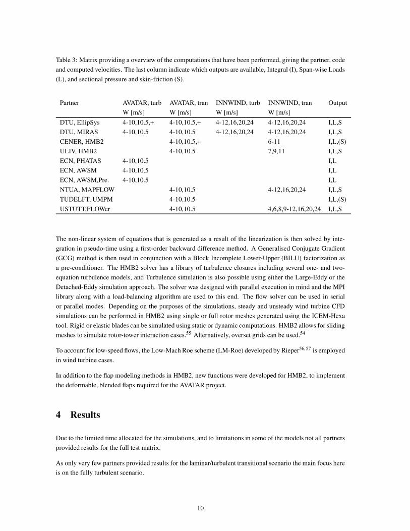
Table 3: Matrix providing a overview of the computations that have been performed, giving the partner, code
and computed velocities. The last column indicate which outputs are available, Integral (I), Span-wise Loads
(L), and sectional pressure and skin-friction (S).
Partner AVATAR, turb AVATAR, tran INNWIND, turb INNWIND, tran Output
W [m/s] W [m/s] W [m/s] W [m/s]
DTU, EllipSys 4-10,10.5,+ 4-10,10.5,+ 4-12,16,20,24 4-12,16,20,24 I,L,S
DTU, MIRAS 4-10,10.5 4-10,10.5 4-12,16,20,24 4-12,16,20,24 I,L,S
CENER, HMB2 4-10,10.5,+ 6-11 I,L,(S)
ULIV, HMB2 4-10,10.5 7,9,11 I,L,S
ECN, PHATAS 4-10,10.5 I,L
ECN, AWSM 4-10,10.5 I,L
ECN, AWSM,Pre. 4-10,10.5 I,L
NTUA, MAPFLOW 4-10,10.5 4-12,16,20,24 I,L,S
TUDELFT, UMPM 4-10,10.5 I,L,(S)
USTUTT,FLOWer 4-10,10.5 4,6,8,9-12,16,20,24 I,L,S
The non-linear system of equations that is generated as a result of the linearization is then solved by inte-
gration in pseudo-time using a first-order backward difference method. A Generalised Conjugate Gradient
(GCG) method is then used in conjunction with a Block Incomplete Lower-Upper (BILU) factorization as
a pre-conditioner. The HMB2 solver has a library of turbulence closures including several one- and two-
equation turbulence models, and Turbulence simulation is also possible using either the Large-Eddy or the
Detached-Eddy simulation approach. The solver was designed with parallel execution in mind and the MPI
library along with a load-balancing algorithm are used to this end. The flow solver can be used in serial
or parallel modes. Depending on the purposes of the simulations, steady and unsteady wind turbine CFD
simulations can be performed in HMB2 using single or full rotor meshes generated using the ICEM-Hexa
tool. Rigid or elastic blades can be simulated using static or dynamic computations. HMB2 allows for sliding
meshes to simulate rotor-tower interaction cases.55 Alternatively, overset grids can be used.54
To account for low-speed flows, the Low-Mach Roe scheme (LM-Roe) developed by Rieper56,57 is employed
in wind turbine cases.
In addition to the flap modeling methods in HMB2, new functions were developed for HMB2, to implement
the deformable, blended flaps required for the AVATAR project.
4 Results
Due to the limited time allocated for the simulations, and to limitations in some of the models not all partners
provided results for the full test matrix.
As only very few partners provided results for the laminar/turbulent transitional scenario the main focus here
is on the fully turbulent scenario.
10

4.1 AVATAR Rotor, transitional
Only three partners delivered results for the laminar/turbulent transitional scenario, but with models cover-
ing the range from a engineering BEM using externally supplied airfoil data, over a Vortex Methods using
internally computed airfoil data to full RANS CFD simulations, the results are believed to provide some
insight.
Looking at the mechanical power Figure 2, and the axial thrust force on the rotor Figure 3, the agreement
acceptable. Comparing the power at 8 and 10 m/s between the ECN AWSM or BEM results and the DTU
EllipSys results a relative difference of 2-3% is observed, while the thrust shows less than 2% error. With
respect to the computed thrust force, the force predicted by the MIRAS solver is lower than the other results.
This is a feature observed in most simulations, and might be connected to the representation of the thick
trailing edge in the vortex method.
0
2000
4000
6000
8000
10000
12000
4 5 6 7 8 9 10
Mec
han
ical
Pow
er [
kW
]
Velocity [m/s]
DTU-ELLDTU-MIRAS
ECN (AWSM)ECN (BEM)
Figure 2: Comparison of the computed mechanical power for the AVATAR reference rotor assuming transi-
tional flow.
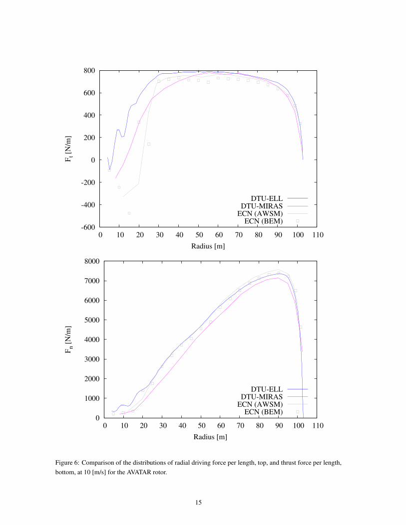
Looking at the radial distribution of the loads in the driving and thrust direction, several things can be ob-
served, see Figure 4 to Figure 6. For the driving forces, the largest deviations are observed in the root area
where separated flow will often be present, while the outboard loads agree quite well for the computed wind
speeds.
For the axial loads, the tendency is that the MIRAS code give the lowest loads, while the AWSM and EllipSys
predicts very similar load distributions.
The location of the transition line can be deduced from the intermittency, which is shown for the suction side
at 5, 8 and 10 [m/s] in Figure 7. Qualitatively, the behavior is correct with a slight movment of the suction
side transition location towards the leading edge with increasing velocity.
11

200
400
600
800
1000
1200
1400
1600
4 5 6 7 8 9 10
Thru
st f
orc
e [k
N]
Velocity [m/s]
DTU-ELLDTU-MIRAS
ECN (AWSM)ECN (BEM)
Figure 3: Comparison of the computed thrust force for the AVATAR reference rotor assuming transitional
flow.
12

-250
-200
-150
-100
-50
0
50
100
150
0 10 20 30 40 50 60 70 80 90 100 110
Ft [N
/m]
Radius [m]
DTU-ELLDTU-MIRAS
ECN (AWSM)ECN (BEM)
-500
0
500
1000
1500
2000
2500
0 10 20 30 40 50 60 70 80 90 100 110
Fn [
N/m
]
Radius [m]
DTU-ELLDTU-MIRAS
ECN (AWSM)ECN (BEM)
Figure 4: Comparison of the distributions of radial driving force per length, top, and thrust force per length,
bottom, at 5 [m/s] for the AVATAR rotor.
13

-400
-300
-200
-100
0
100
200
300
400
500
600
0 10 20 30 40 50 60 70 80 90 100 110
Ft [N
/m]
Radius [m]
DTU-ELLDTU-MIRAS
ECN (AWSM)ECN (BEM)
0
500
1000
1500
2000
2500
3000
3500
4000
4500
5000
0 10 20 30 40 50 60 70 80 90 100 110
Fn [
N/m
]
Radius [m]
DTU-ELLDTU-MIRAS
ECN (AWSM)ECN (BEM)
Figure 5: Comparison of the distributions of radial driving force per length, top, and thrust force per length,
bottom, at 8 [m/s] for the AVATAR rotor.
14
-600
-400
-200
0
200
400
600
800
0 10 20 30 40 50 60 70 80 90 100 110
Ft [N
/m]
Radius [m]
DTU-ELLDTU-MIRAS
ECN (AWSM)ECN (BEM)
0
1000
2000
3000
4000
5000
6000
7000
8000
0 10 20 30 40 50 60 70 80 90 100 110
Fn [
N/m
]
Radius [m]
DTU-ELLDTU-MIRAS
ECN (AWSM)ECN (BEM)
Figure 6: Comparison of the distributions of radial driving force per length, top, and thrust force per length,
bottom, at 10 [m/s] for the AVATAR rotor.
15

Figure 7: Development of the transition location visualized by the intermittency at the suction side of the
AVATAR blade for a wind speed of 5, 8, and 10 [m/s], from top to bottom. The expected forward movment
of the transition line can be seen as a weak movement of the red area towards the leading edge, plots are
based on EllipSys3D computations.
16

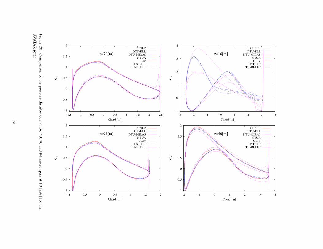
4.2 AVATAR Rotor, fully turbulent
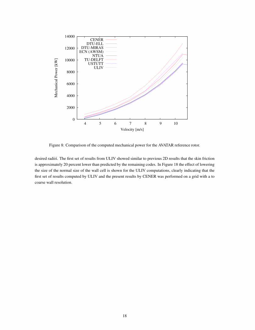
I the present section, the fully turbulent computations will be evaluated. Starting with the integral quantities
in the form of mechanical power and thrust, see Figure 8 and 9. For the mechanical power the curves are
basically distributed in three groups, the inviscid UMPM code by TU-DELFT predicts the highest power in
good agreement with the neglected friction. The MIRAS and the incompressible EllipSys code of DTU which
agreed well with the ECN engineering models for transitional flow, predicts lower power when switching
from fully turbulent to transitional computations, due to lower friction in the laminar parts of the flow. The
FLOWer code used by USTUTT and the MAPFLOW code by NTUA agrees well with the EllipSys and
MIRAS results, while the HMB2 by ULIV and CENER predicts higher power than the transitional results
predicted by the AWSM model by ECN. The ECN AWSM results based on transitional airfoil data are
included here as reference, to allow comparison between the fully turbulent and transitional results.
As it is not known if the ECN results are the correct answer, all that can be stated is that the MIRAS and
EllipSys computations perform qualitatively correct when switching from laminar/turbulent transitional con-
ditions to fully turbulent flow, by predicting lower production for the fully turbulent case. The fact that the
HMB2 by CENER over predicts the power production, is assumed mainly to be caused by the HMB2 code
predicting higher suction in the leading edge region of the airfoil, which must be one of the reasons that these
code predicts the highest mechanical power. For the HMB2 this is observed both on the grid by CENER and
on the refined grid by ULIV.
Whether this is connected to problems of handling high Re and low Mach, or connected to some other reason
like turbulence modelling is not clear. But even for the cases where the CENER simulations are based on the
k−ω SST model by Menter, similar to the EllipSys and FLOWer simulations, the results do not agree.
Looking at the thrust force in Figure 9, generally the agreement between the codes are much closer grouping
below the ECN engineering results with the exception of the inviscid UPMP code lying high above and the
MIRAS code lying far below the ECN results.
Two of the partners provided grid in dependency test, and Figure 11 and Figure 10 showing the solution for
the MAPFLOW and EllipSys on the common grid and on a grid which is coarsened by a factor two in all
direction, indicate that the grid dependency of these individual codes are much smaller than the difference
between the codes.
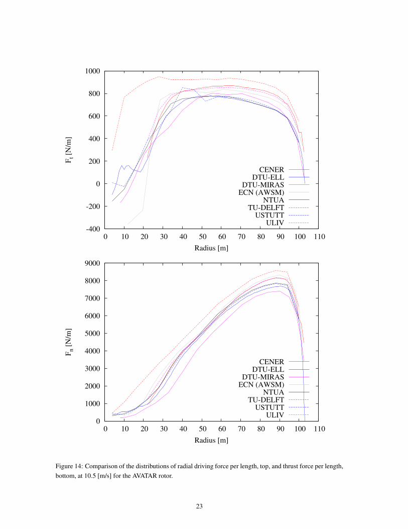
Comparing the radial distributions of the loads in driving and thrust direction as seen in the Figures 12 to 14,
the picture is more complicated and might indicate that not all data are processed in exactly the same way.
Unfortunately, at present time it is not possible to further pursue this problem. Generally, the MAPFLOW,
FLOWer and EllipSys3D results are very close with respect to the driving force.
Finally, looking at the detailed pressure and skin friction distributions, a good qualitative agreement is ob-
served, see Figures 15 to 21. At the innermost section where the thickest airfoils are located the two vortex
methods UPMP and MIRAS show large deviations from the other codes, additionally the HMB2 results were
not reported here due to convergence problems. On the outer part of the blade, the HMB2 and MAPFLOW
codes predicts higher suction than the remaining solvers,
Generally, the skin friction curves agrees well between four of the code, the FLOWer code by USTUTT,
MAPFLOW by NTUA, the EllipSys3D results by DTU and the HMB2 results by ULIV. For the remaining
partners TU-DELFT did not provide results due to the code being inviscid, CENER did not provide data
due to problems with the skin friction level, and DTU did not provide results for the MIRAS code at the
17
0
2000
4000
6000
8000
10000
12000
14000
4 5 6 7 8 9 10
Mec
han
ical
Pow
er [
kW
]
Velocity [m/s]
CENERDTU-ELL
DTU-MIRASECN (AWSM)
NTUATU-DELFT
USTUTTULIV
Figure 8: Comparison of the computed mechanical power for the AVATAR reference rotor.
desired radiis. The first set of results from ULIV showed similar to previous 2D results that the skin friction
is approximately 20 percent lower than predicted by the remaining codes. In Figure 18 the effect of lowering
the size of the normal size of the wall cell is shown for the ULIV computations, clearly indicating that the
first set of results computed by ULIV and the present results by CENER was performed on a grid with a to
coarse wall resolution.
18

0
200
400
600
800
1000
1200
1400
1600
1800
4 5 6 7 8 9 10
Thru
st f
orc
e [k
N]
Velocity [m/s]
CENERDTU-ELL
DTU-MIRASECN (AWSM)
NTUATU-DELFT
USTUTTULIV
Figure 9: Comparison of the computed thrust force for the AVATAR reference rotor.
0
1000
2000
3000
4000
5000
6000
7000
8000
9000
10000
4 5 6 7 8 9 10
Mec
han
ical
Pow
er [
kW
]
Velocity [m/s]
DTU-ELLDTU-ELL
NTUANTUA
Figure 10: Comparison of the computed mechanical power force for the AVATAR reference rotor, using two
grid levels. The fine grid level is indicated by the full drawn lines.
19

200
400
600
800
1000
1200
1400
1600
4 5 6 7 8 9 10
Thru
st f
orc
e [k
N]
Velocity [m/s]
DTU-ELLDTU-ELL
NTUANTUA
Figure 11: Comparison of the computed thrust force for the AVATAR reference rotor, using two grid levels.
The fine grid level is indicated by the full drawn lines.
20

-250
-200
-150
-100
-50
0
50
100
0 10 20 30 40 50 60 70 80 90 100 110
Ft [N
/m]
Radius [m]
CENERDTU-ELL
DTU-MIRASECN (AWSM)
NTUATU-DELFT
USTUTTULIV
-500
0
500
1000
1500
2000
0 10 20 30 40 50 60 70 80 90 100 110
Fn [
N/m
]
Radius [m]
CENERDTU-ELL
DTU-MIRASECN (AWSM)
NTUATU-DELFT
USTUTTULIV
Figure 12: Comparison of the distributions of radial driving force per length, top, and thrust force per length,
bottom, at 4 [m/s] for the AVATAR rotor.
21

-300
-200
-100
0
100
200
300
400
500
600
0 10 20 30 40 50 60 70 80 90 100 110
Ft [N
/m]
Radius [m]
CENERDTU-ELL
DTU-MIRASECN (AWSM)
NTUATU-DELFT
USTUTTULIV
0
500
1000
1500
2000
2500
3000
3500
4000
4500
5000
0 10 20 30 40 50 60 70 80 90 100 110
Fn [
N/m
]
Radius [m]
CENERDTU-ELL
DTU-MIRASECN (AWSM)
NTUATU-DELFT
USTUTTULIV
Figure 13: Comparison of the distributions of radial driving force per length, top, and thrust force per length,
bottom, at 8 [m/s] for the AVATAR rotor.
22
-400
-200
0
200
400
600
800
1000
0 10 20 30 40 50 60 70 80 90 100 110
Ft [N
/m]
Radius [m]
CENERDTU-ELL
DTU-MIRASECN (AWSM)
NTUATU-DELFT
USTUTTULIV
0
1000
2000
3000
4000
5000
6000
7000
8000
9000
0 10 20 30 40 50 60 70 80 90 100 110
Fn [
N/m
]
Radius [m]
CENERDTU-ELL
DTU-MIRASECN (AWSM)
NTUATU-DELFT
USTUTTULIV
Figure 14: Comparison of the distributions of radial driving force per length, top, and thrust force per length,
bottom, at 10.5 [m/s] for the AVATAR rotor.
23

-1
0
1
2
3
4
-3 -2 -1 0 1 2 3 4
-Cp
Chord [m]
CENERDTU-ELL
DTU-MIRASNTUAULIV
USTUTTTU-DELFT
r=16[m]
-1
-0.5
0
0.5
1
1.5
2
-2 -1 0 1 2 3 4
-Cp
Chord [m]
CENERDTU-ELL
DTU-MIRASNTUAULIV
USTUTTTU-DELFT
r=40[m]
-1
-0.5
0
0.5
1
1.5
2
-1.5 -1 -0.5 0 0.5 1 1.5 2 2.5
-Cp
Chord [m]
CENERDTU-ELL
DTU-MIRASNTUAULIV
USTUTTTU-DELFT
r=70[m]
-1
-0.5
0
0.5
1
1.5
2
-1 -0.5 0 0.5 1 1.5 2
-Cp
Chord [m]
CENERDTU-ELL
DTU-MIRASNTUAULIV
USTUTTTU-DELFT
r=94[m]
Fig
ure
15
:C
om
pariso
no
fth
ep
ressure
distrib
utio
ns
at1
6,
40
,7
0an
d9
4m
etersp
anat
4[m
/s]fo
rth
e
AV
AT
AR
roto
r.
24

0
0.002
0.004
0.006
0.008
0.01
0.012
0.014
-3 -2 -1 0 1 2 3 4
Cf
Chord [m]
CENERDTU-ELL
DTU-MIRASNTUAULIV
USTUTTTU-DELFT
r=16[m]
0
0.001
0.002
0.003
0.004
0.005
0.006
0.007
0.008
-2 -1 0 1 2 3 4
Cf
Chord [m]
CENERDTU-ELL
DTU-MIRASNTUAULIV
USTUTTTU-DELFT
r=40[m]
0
0.001
0.002
0.003
0.004
0.005
0.006
0.007
-1.5 -1 -0.5 0 0.5 1 1.5 2 2.5
Cf
Chord [m]
CENERDTU-ELL
DTU-MIRASNTUAULIV
USTUTTTU-DELFT
r=70[m]
0
0.001
0.002
0.003
0.004
0.005
0.006
-1 -0.5 0 0.5 1 1.5 2
Cf
Chord [m]
CENERDTU-ELL
DTU-MIRASNTUAULIV
USTUTTTU-DELFT
r=94[m]
Fig
ure
16
:C
om
pariso
no
fth
esk
infrictio
nd
istribu
tion
sat
16
,4
0,
70
and
94
meter
span
at5
[m/s]
for
the
AV
AT
AR
roto
r.
25

-1
0
1
2
3
4
-3 -2 -1 0 1 2 3 4
-Cp
Chord [m]
CENERDTU-ELL
DTU-MIRASNTUAULIV
USTUTTTU-DELFT
r=16[m]
-1
-0.5
0
0.5
1
1.5
2
-2 -1 0 1 2 3 4
-Cp
Chord [m]
CENERDTU-ELL
DTU-MIRASNTUAULIV
USTUTTTU-DELFT
r=40[m]
-1
-0.5
0
0.5
1
1.5
2
-1.5 -1 -0.5 0 0.5 1 1.5 2 2.5
-Cp
Chord [m]
CENERDTU-ELL
DTU-MIRASNTUAULIV
USTUTTTU-DELFT
r=70[m]
-1
-0.5
0
0.5
1
1.5
2
-1 -0.5 0 0.5 1 1.5 2
-Cp
Chord [m]
CENERDTU-ELL
DTU-MIRASNTUAULIV
USTUTTTU-DELFT
r=94[m]
Fig
ure
17
:C
om
pariso
no
fth
ep
ressure
distrib
utio
ns
at1
6,
40
,7
0an
d9
4m
etersp
anat
8[m
/s]fo
rth
e
AV
AT
AR
roto
r.
26

0
0.001
0.002
0.003
0.004
0.005
0.006
0.007
0.008
0.009
0.01
-2 -1 0 1 2 3 4
Cf
Chord [m]
DTU-ELLDTU-MIRAS
NTUAULIV
USTUTTTU-DELFT
ULIVULIV, coarse
Figure 18: Comparison of the skin friction distributions at 40 meter span at 8 [m/s] for the AVATAR rotor
illustrating the dramatical effect of refining the grid for the HMB code.
27

0
0.002
0.004
0.006
0.008
0.01
0.012
0.014
-3 -2 -1 0 1 2 3 4
Cf
Chord [m]
CENERDTU-ELL
DTU-MIRASNTUAULIV
USTUTTTU-DELFT
r=16[m]
0
0.001
0.002
0.003
0.004
0.005
0.006
0.007
0.008
0.009
0.01
-2 -1 0 1 2 3 4
Cf
Chord [m]
CENERDTU-ELL
DTU-MIRASNTUAULIV
USTUTTTU-DELFT
r=40[m]
0
0.001
0.002
0.003
0.004
0.005
0.006
0.007
-1.5 -1 -0.5 0 0.5 1 1.5 2 2.5
Cf
Chord [m]
CENERDTU-ELL
DTU-MIRASNTUAULIV
USTUTTTU-DELFT
r=70[m]
0
0.001
0.002
0.003
0.004
0.005
0.006
0.007
-1 -0.5 0 0.5 1 1.5 2
Cf
Chord [m]
CENERDTU-ELL
DTU-MIRASNTUAULIV
USTUTTTU-DELFT
r=94[m]
Fig
ure
19
:C
om
pariso
no
fth
esk
infrictio
nd
istribu
tion
sat
16
,4
0,
70
and
94
meter
span
at8
[m/s]
for
the
AV
AT
AR
roto
r.
28
-1
0
1
2
3
4
-3 -2 -1 0 1 2 3 4
-Cp
Chord [m]
CENERDTU-ELL
DTU-MIRASNTUAULIV
USTUTTTU-DELFT
r=16[m]
-1
-0.5
0
0.5
1
1.5
2
-2 -1 0 1 2 3 4
-Cp
Chord [m]
CENERDTU-ELL
DTU-MIRASNTUAULIV
USTUTTTU-DELFT
r=40[m]
-1
-0.5
0
0.5
1
1.5
2
-1.5 -1 -0.5 0 0.5 1 1.5 2 2.5
-Cp
Chord [m]
CENERDTU-ELL
DTU-MIRASNTUAULIV
USTUTTTU-DELFT
r=70[m]
-1
-0.5
0
0.5
1
1.5
2
-1 -0.5 0 0.5 1 1.5 2
-Cp
Chord [m]
CENERDTU-ELL
DTU-MIRASNTUAULIV
USTUTTTU-DELFT
r=94[m]
Fig
ure
20
:C
om
pariso
no
fth
ep
ressure
distrib
utio
ns
at1
6,
40
,7
0an
d9
4m
etersp
anat
10
[m/s]
for
the
AV
AT
AR
roto
r.
29

0
0.002
0.004
0.006
0.008
0.01
0.012
0.014
-3 -2 -1 0 1 2 3 4
Cf
Chord [m]
CENERDTU-ELL
DTU-MIRASNTUAULIV
USTUTTTU-DELFT
r=16[m]
0
0.001
0.002
0.003
0.004
0.005
0.006
0.007
0.008
0.009
-2 -1 0 1 2 3 4
Cf
Chord [m]
CENERDTU-ELL
DTU-MIRASNTUAULIV
USTUTTTU-DELFT
r=40[m]
0
0.001
0.002
0.003
0.004
0.005
0.006
0.007
-1.5 -1 -0.5 0 0.5 1 1.5 2 2.5
Cf
Chord [m]
CENERDTU-ELL
DTU-MIRASNTUAULIV
USTUTTTU-DELFT
r=70[m]
0
0.001
0.002
0.003
0.004
0.005
0.006
-1 -0.5 0 0.5 1 1.5 2
Cf
Chord [m]
CENERDTU-ELL
DTU-MIRASNTUAULIV
USTUTTTU-DELFT
r=94[m]
Fig
ure
21
:C
om
pariso
no
fth
esk
infrictio
nd
istribu
tion
sat
16
,4
0,
70
and
94
meter
span
at1
0[m
/s]fo
rth
e
AV
AT
AR
roto
r.
30

4.3 INNWIND/DTU-10MWRotor, turbulent conditions
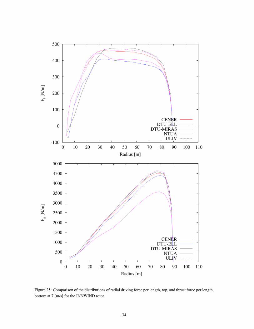
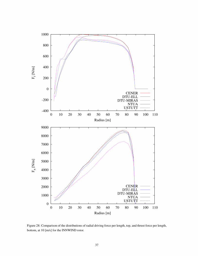
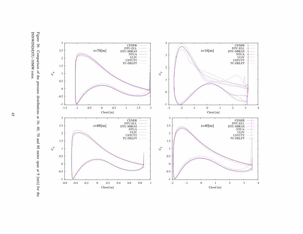
For the INNWIND/DTU-10MW rotor the picture is similar to the one seen for the AVATAR rotor, though
with a tendency to a better agreement between the codes than observed for the AVATAR rotor. It must be
said that there are fewer results available for this case, and some of the codes producing the outliers from the
AVATAR comparison are not available in the present comparison.
For the power curve, the agreement up to 10 m/s is decent, while the agreement for the thrust curve is similar
to the one observed for the AVATAR rotor, see Figures 22 and 23. Above 10 m/s a tendency similar to that
observed for the AVATAR rotor, namely that the FLOWer and EllipSys3D show good agreement between
each other, while the preconditioned MAPFLOW predict higher power.
The agreement between the radial distribution of the driving loads is again arranged in groups, with two of
the compressible solvers HMB2 by ULIV and MAPFLOW by NTUA predicting the highest driving force,
FLOWer simulations from USTUTT and EllipSys simulation from DTU mutually agreeing well, and MIRAS
predicting the lowest power, see Figures 24 to 29.
The normal force predicted by the MIRAS code is consistent with the observations from the AVATAR rotor,
where it also predicts lower thrust compared to the remaining solvers, see Figure 24 and 29. For the pressure
and skin friction good agreement is observed between the USTUTT and DTU results, see Figure 30 to 39,
here the NTUA code predicts higher suction peak especially at the outboard sections for the higher wind
speeds.
0
2000
4000
6000
8000
10000
12000
14000
0 5 10 15 20 25
Mec
han
ical
Pow
er [
kW
]
Wind Speed [m/s]
CENERDTU-ELL
DTU-MIRASNTUA
USTUTTULIV
Figure 22: Comparison of the computed mechanical power for the INNWIND/DTU 10MW reference rotor.
31

0
200
400
600
800
1000
1200
1400
1600
1800
0 5 10 15 20 25
Thru
st [
kN
]
Wind Speed [m/s]
CENERDTU-ELL
DTU-MIRASNTUA
USTUTTULIV
Figure 23: Comparison of the computed thrust force for the INNWIND/DTU 10MW reference rotor.
32

-100
-50
0
50
100
150
200
250
300
350
0 10 20 30 40 50 60 70 80 90 100 110
Ft [N
/m]
Radius [m]
CENERDTU-ELL
DTU-MIRASNTUA
USTUTT
0
500
1000
1500
2000
2500
3000
3500
4000
0 10 20 30 40 50 60 70 80 90 100 110
Fn [
N/m
]
Radius [m]
CENERDTU-ELL
DTU-MIRASNTUA
USTUTT
Figure 24: Comparison of the distributions of radial driving force per length, top, and thrust force per length,
bottom at 6 [m/s] for the INNWIND rotor.
33
-100
0
100
200
300
400
500
0 10 20 30 40 50 60 70 80 90 100 110
Ft [N
/m]
Radius [m]
CENERDTU-ELL
DTU-MIRASNTUAULIV
0
500
1000
1500
2000
2500
3000
3500
4000
4500
5000
0 10 20 30 40 50 60 70 80 90 100 110
Fn [
N/m
]
Radius [m]
CENERDTU-ELL
DTU-MIRASNTUAULIV
Figure 25: Comparison of the distributions of radial driving force per length, top, and thrust force per length,
bottom at 7 [m/s] for the INNWIND rotor.
34

-200
-100
0
100
200
300
400
500
600
700
0 10 20 30 40 50 60 70 80 90 100 110
Ft [N
/m]
Radius [m]
CENERDTU-ELL
DTU-MIRASNTUA
USTUTT
0
1000
2000
3000
4000
5000
6000
0 10 20 30 40 50 60 70 80 90 100 110
Fn [
N/m
]
Radius [m]
CENERDTU-ELL
DTU-MIRASNTUA
USTUTT
Figure 26: Comparison of the distributions of radial driving force per length, top, and thrust force per length,
bottom, at 8 [m/s] for the INNWIND rotor.
35

-200
0
200
400
600
800
1000
0 10 20 30 40 50 60 70 80 90 100 110
Ft [N
/m]
Radius [m]
CENERDTU-ELL
DTU-MIRASNTUA
USTUTTULIV
0
1000
2000
3000
4000
5000
6000
7000
8000
0 10 20 30 40 50 60 70 80 90 100 110
Fn [
N/m
]
Radius [m]
CENERDTU-ELL
DTU-MIRASNTUA
USTUTTULIV
Figure 27: Comparison of the distributions of radial driving force per length, top, and thrust force per length,
bottom, at 9 [m/s] for the INNWIND rotor.
36
-400
-200
0
200
400
600
800
1000
0 10 20 30 40 50 60 70 80 90 100 110
Ft [N
/m]
Radius [m]
CENERDTU-ELL
DTU-MIRASNTUA
USTUTT
0
1000
2000
3000
4000
5000
6000
7000
8000
9000
0 10 20 30 40 50 60 70 80 90 100 110
Fn [
N/m
]
Radius [m]
CENERDTU-ELL
DTU-MIRASNTUA
USTUTT
Figure 28: Comparison of the distributions of radial driving force per length, top, and thrust force per length,
bottom, at 10 [m/s] for the INNWIND rotor.
37

-400
-200
0
200
400
600
800
1000
1200
1400
0 10 20 30 40 50 60 70 80 90 100 110
Ft [N
/m]
Radius [m]
CENERDTU-ELL
DTU-MIRASNTUA
USTUTTULIV
0
2000
4000
6000
8000
10000
12000
0 10 20 30 40 50 60 70 80 90 100 110
Fn [
N/m
]
Radius [m]
CENERDTU-ELL
DTU-MIRASNTUA
USTUTTULIV
Figure 29: Comparison of the distributions of radial driving force per length, top, and thrust force per length,
bottom, at 11 [m/s] for the INNWIND rotor.
38

-1
0
1
2
3
4
-3 -2 -1 0 1 2 3 4
-Cp
Chord [m]
CENERDTU-ELL
DTU-MIRASNTUAULIV
USTUTTTU-DELFT
r=16[m]
-1
-0.5
0
0.5
1
1.5
2
-2 -1 0 1 2 3 4
-Cp
Chord [m]
CENERDTU-ELL
DTU-MIRASNTUAULIV
USTUTTTU-DELFT
r=40[m]
-1
-0.5
0
0.5
1
1.5
2
-1.5 -1 -0.5 0 0.5 1 1.5 2
-Cp
Chord [m]
CENERDTU-ELL
DTU-MIRASNTUAULIV
USTUTTTU-DELFT
r=70[m]
-1
-0.5
0
0.5
1
1.5
2
-0.6 -0.4 -0.2 0 0.2 0.4 0.6 0.8 1
-Cp
Chord [m]
CENERDTU-ELL
DTU-MIRASNTUAULIV
USTUTTTU-DELFT
r=88[m]
Fig
ure
30
:C
om
pariso
no
fth
ep
ressure
distrib
utio
ns
at1
6,
40
,7
0an
d8
8m
etersp
anat
6[m
/s]fo
rth
e
INN
WIN
D/D
TU
-10
MW
roto
r.
39

0
0.002
0.004
0.006
0.008
0.01
0.012
0.014
0.016
-3 -2 -1 0 1 2 3 4
Cf
Chord [m]
CENERDTU-ELL
DTU-MIRASNTUAULIV
USTUTTTU-DELFT
r=16[m]
0
0.001
0.002
0.003
0.004
0.005
0.006
0.007
0.008
0.009
-2 -1 0 1 2 3 4
Cf
Chord [m]
CENERDTU-ELL
DTU-MIRASNTUAULIV
USTUTTTU-DELFT
r=40[m]
0
0.002
0.004
0.006
0.008
0.01
0.012
-1.5 -1 -0.5 0 0.5 1 1.5 2
Cf
Chord [m]
CENERDTU-ELL
DTU-MIRASNTUAULIV
USTUTTTU-DELFT
r=70[m]
0
0.001
0.002
0.003
0.004
0.005
0.006
0.007
0.008
0.009
0.01
-0.6 -0.4 -0.2 0 0.2 0.4 0.6 0.8 1
Cf
Chord [m]
CENERDTU-ELL
DTU-MIRASNTUAULIV
USTUTTTU-DELFT
r=88[m]
Fig
ure
31
:C
om
pariso
no
fth
esk
infrictio
nd
istribu
tion
sat
16
,4
0,
70
and
88
meter
span
at6
[m/s]
for
the
INN
WIN
D/D
TU
-10
MW
roto
r.
40

-1
0
1
2
3
4
-3 -2 -1 0 1 2 3 4
-Cp
Chord [m]
CENERDTU-ELL
DTU-MIRASNTUAULIV
USTUTTTU-DELFT
r=16[m]
-1
-0.5
0
0.5
1
1.5
2
2.5
3
-2 -1 0 1 2 3 4
-Cp
Chord [m]
CENERDTU-ELL
DTU-MIRASNTUAULIV
USTUTTTU-DELFT
r=40[m]
-1
-0.5
0
0.5
1
1.5
2
2.5
3
-1.5 -1 -0.5 0 0.5 1 1.5 2
-Cp
Chord [m]
CENERDTU-ELL
DTU-MIRASNTUAULIV
USTUTTTU-DELFT
r=70[m]
-1
-0.5
0
0.5
1
1.5
2
2.5
3
-0.6 -0.4 -0.2 0 0.2 0.4 0.6 0.8 1
-Cp
Chord [m]
CENERDTU-ELL
DTU-MIRASNTUAULIV
USTUTTTU-DELFT
r=88[m]
Fig
ure
32
:C
om
pariso
no
fth
ep
ressure
distrib
utio
ns
at1
6,
40
,7
0an
d8
8m
etersp
anat
7[m
/s]fo
rth
e
INN
WIN
D/D
TU
-10
MW
roto
r.
41

0
0.002
0.004
0.006
0.008
0.01
0.012
0.014
0.016
0.018
-3 -2 -1 0 1 2 3 4
Cf
Chord [m]
CENERDTU-ELL
DTU-MIRASNTUAULIV
USTUTTTU-DELFT
r=16[m]
0
0.002
0.004
0.006
0.008
0.01
0.012
-2 -1 0 1 2 3 4
Cf
Chord [m]
CENERDTU-ELL
DTU-MIRASNTUAULIV
USTUTTTU-DELFT
r=40[m]
0
0.002
0.004
0.006
0.008
0.01
0.012
0.014
-1.5 -1 -0.5 0 0.5 1 1.5 2
Cf
Chord [m]
CENERDTU-ELL
DTU-MIRASNTUAULIV
USTUTTTU-DELFT
r=70[m]
0
0.002
0.004
0.006
0.008
0.01
0.012
0.014
-0.6 -0.4 -0.2 0 0.2 0.4 0.6 0.8 1
Cf
Chord [m]
CENERDTU-ELL
DTU-MIRASNTUAULIV
USTUTTTU-DELFT
r=88[m]
Fig
ure
33
:C
om
pariso
no
fth
esk
infrictio
nd
istribu
tion
sat
16
,4
0,
70
and
88
meter
span
at7
[m/s]
for
the
INN
WIN
D/D
TU
-10
MW
roto
r.
42

-1
0
1
2
3
4
-3 -2 -1 0 1 2 3 4
-Cp
Chord [m]
CENERDTU-ELL
DTU-MIRASNTUAULIV
USTUTTTU-DELFT
r=16[m]
-1
-0.5
0
0.5
1
1.5
2
2.5
3
-2 -1 0 1 2 3 4
-Cp
Chord [m]
CENERDTU-ELL
DTU-MIRASNTUAULIV
USTUTTTU-DELFT
r=40[m]
-1
-0.5
0
0.5
1
1.5
2
2.5
3
-1.5 -1 -0.5 0 0.5 1 1.5 2
-Cp
Chord [m]
CENERDTU-ELL
DTU-MIRASNTUAULIV
USTUTTTU-DELFT
r=70[m]
-1
-0.5
0
0.5
1
1.5
2
2.5
3
-0.6 -0.4 -0.2 0 0.2 0.4 0.6 0.8 1
-Cp
Chord [m]
CENERDTU-ELL
DTU-MIRASNTUAULIV
USTUTTTU-DELFT
r=88[m]
Fig
ure
34
:C
om
pariso
no
fth
ep
ressure
distrib
utio
ns
at1
6,
40
,7
0an
d8
8m
etersp
anat
8[m
/s]fo
rth
e
INN
WIN
D/D
TU
-10
MW
roto
r.
43

0
0.002
0.004
0.006
0.008
0.01
0.012
0.014
0.016
-3 -2 -1 0 1 2 3 4
Cf
Chord [m]
CENERDTU-ELL
DTU-MIRASNTUAULIV
USTUTTTU-DELFT
r=16[m]
0
0.002
0.004
0.006
0.008
0.01
0.012
-2 -1 0 1 2 3 4
Cf
Chord [m]
CENERDTU-ELL
DTU-MIRASNTUAULIV
USTUTTTU-DELFT
r=40[m]
0
0.002
0.004
0.006
0.008
0.01
0.012
-1.5 -1 -0.5 0 0.5 1 1.5 2
Cf
Chord [m]
CENERDTU-ELL
DTU-MIRASNTUAULIV
USTUTTTU-DELFT
r=70[m]
0
0.002
0.004
0.006
0.008
0.01
0.012
-0.6 -0.4 -0.2 0 0.2 0.4 0.6 0.8 1
Cf
Chord [m]
CENERDTU-ELL
DTU-MIRASNTUAULIV
USTUTTTU-DELFT
r=88[m]
Fig
ure
35
:C
om
pariso
no
fth
esk
infrictio
nd
istribu
tion
sat
16
,4
0,
70
and
88
meter
span
at8
[m/s]
for
the
INN
WIN
D/D
TU
-10
MW
roto
r.
44
-1
0
1
2
3
4
-3 -2 -1 0 1 2 3 4
-Cp
Chord [m]
CENERDTU-ELL
DTU-MIRASNTUAULIV
USTUTTTU-DELFT
r=16[m]
-1
-0.5
0
0.5
1
1.5
2
2.5
3
-2 -1 0 1 2 3 4
-Cp
Chord [m]
CENERDTU-ELL
DTU-MIRASNTUAULIV
USTUTTTU-DELFT
r=40[m]
-1
-0.5
0
0.5
1
1.5
2
2.5
3
-1.5 -1 -0.5 0 0.5 1 1.5 2
-Cp
Chord [m]
CENERDTU-ELL
DTU-MIRASNTUAULIV
USTUTTTU-DELFT
r=70[m]
-1
-0.5
0
0.5
1
1.5
2
2.5
3
-0.6 -0.4 -0.2 0 0.2 0.4 0.6 0.8 1
-Cp
Chord [m]
CENERDTU-ELL
DTU-MIRASNTUAULIV
USTUTTTU-DELFT
r=88[m]
Fig
ure
36
:C
om
pariso
no
fth
ep
ressure
distrib
utio
ns
at1
6,
40
,7
0an
d8
8m
etersp
anat
9[m
/s]fo
rth
e
INN
WIN
D/D
TU
-10
MW
roto
r.
45

0
0.002
0.004
0.006
0.008
0.01
0.012
0.014
0.016
0.018
-3 -2 -1 0 1 2 3 4
Cf
Chord [m]
CENERDTU-ELL
DTU-MIRASNTUAULIV
USTUTTTU-DELFT
r=16[m]
0
0.002
0.004
0.006
0.008
0.01
0.012
0.014
-2 -1 0 1 2 3 4
Cf
Chord [m]
CENERDTU-ELL
DTU-MIRASNTUAULIV
USTUTTTU-DELFT
r=40[m]
0
0.002
0.004
0.006
0.008
0.01
0.012
0.014
-1.5 -1 -0.5 0 0.5 1 1.5 2
Cf
Chord [m]
CENERDTU-ELL
DTU-MIRASNTUAULIV
USTUTTTU-DELFT
r=70[m]
0
0.002
0.004
0.006
0.008
0.01
0.012
0.014
-0.6 -0.4 -0.2 0 0.2 0.4 0.6 0.8 1
Cf
Chord [m]
CENERDTU-ELL
DTU-MIRASNTUAULIV
USTUTTTU-DELFT
r=88[m]
Fig
ure
37
:C
om
pariso
no
fth
esk
infrictio
nd
istribu
tion
sat
16
,4
0,
70
and
88
meter
span
at9
[m/s]
for
the
INN
WIN
D/D
TU
-10
MW
roto
r.
46

-1
0
1
2
3
4
-3 -2 -1 0 1 2 3 4
-Cp
Chord [m]
CENERDTU-ELL
DTU-MIRASNTUAULIV
USTUTTTU-DELFT
r=16[m]
-1
-0.5
0
0.5
1
1.5
2
2.5
3
-2 -1 0 1 2 3 4
-Cp
Chord [m]
CENERDTU-ELL
DTU-MIRASNTUAULIV
USTUTTTU-DELFT
r=40[m]
-1
-0.5
0
0.5
1
1.5
2
2.5
3
-1.5 -1 -0.5 0 0.5 1 1.5 2
-Cp
Chord [m]
CENERDTU-ELL
DTU-MIRASNTUAULIV
USTUTTTU-DELFT
r=70[m]
-1
-0.5
0
0.5
1
1.5
2
2.5
3
-0.6 -0.4 -0.2 0 0.2 0.4 0.6 0.8 1
-Cp
Chord [m]
CENERDTU-ELL
DTU-MIRASNTUAULIV
USTUTTTU-DELFT
r=88[m]
Fig
ure
38
:C
om
pariso
no
fth
ep
ressure
distrib
utio
ns
at1
6,
40
,7
0an
d8
8m
etersp
anat
10
[m/s]
for
the
INN
WIN
D/D
TU
-10
MW
roto
r.
47

0
0.002
0.004
0.006
0.008
0.01
0.012
0.014
0.016
-3 -2 -1 0 1 2 3 4
Cf
Chord [m]
CENERDTU-ELL
DTU-MIRASNTUAULIV
USTUTTTU-DELFT
r=16[m]
0
0.001
0.002
0.003
0.004
0.005
0.006
0.007
0.008
0.009
0.01
-2 -1 0 1 2 3 4
Cf
Chord [m]
CENERDTU-ELL
DTU-MIRASNTUAULIV
USTUTTTU-DELFT
r=40[m]
0
0.002
0.004
0.006
0.008
0.01
0.012
0.014
-1.5 -1 -0.5 0 0.5 1 1.5 2
Cf
Chord [m]
CENERDTU-ELL
DTU-MIRASNTUAULIV
USTUTTTU-DELFT
r=70[m]
0
0.002
0.004
0.006
0.008
0.01
0.012
-0.6 -0.4 -0.2 0 0.2 0.4 0.6 0.8 1
Cf
Chord [m]
CENERDTU-ELL
DTU-MIRASNTUAULIV
USTUTTTU-DELFT
r=88[m]
Fig
ure
39
:C
om
pariso
no
fth
esk
infrictio
nd
istribu
tion
sat
16
,4
0,
70
and
88
meter
span
at1
0[m
/s]fo
rth
e
INN
WIN
D/D
TU
-10
MW
roto
r.
48

-1
0
1
2
3
4
-3 -2 -1 0 1 2 3 4
-Cp
Chord [m]
CENERDTU-ELL
DTU-MIRASNTUAULIV
USTUTTTU-DELFT
r=16[m]
-1
-0.5
0
0.5
1
1.5
2
2.5
3
-2 -1 0 1 2 3 4
-Cp
Chord [m]
CENERDTU-ELL
DTU-MIRASNTUAULIV
USTUTTTU-DELFT
r=40[m]
-1
-0.5
0
0.5
1
1.5
2
2.5
3
-1.5 -1 -0.5 0 0.5 1 1.5 2
-Cp
Chord [m]
CENERDTU-ELL
DTU-MIRASNTUAULIV
USTUTTTU-DELFT
r=70[m]
-1
-0.5
0
0.5
1
1.5
2
2.5
3
-0.6 -0.4 -0.2 0 0.2 0.4 0.6 0.8 1
-Cp
Chord [m]
CENERDTU-ELL
DTU-MIRASNTUAULIV
USTUTTTU-DELFT
r=88[m]
Fig
ure
40
:C
om
pariso
no
fth
ep
ressure
distrib
utio
ns
at1
6,
40
,7
0an
d8
8m
etersp
anat
10
[m/s]
for
the
INN
WIN
D/D
TU
-10
MW
roto
r.
49

0
0.002
0.004
0.006
0.008
0.01
0.012
0.014
0.016
-3 -2 -1 0 1 2 3 4
Cf
Chord [m]
CENERDTU-ELL
DTU-MIRASNTUAULIV
USTUTTTU-DELFT
r=16[m]
0
0.001
0.002
0.003
0.004
0.005
0.006
0.007
0.008
0.009
0.01
-2 -1 0 1 2 3 4
Cf
Chord [m]
CENERDTU-ELL
DTU-MIRASNTUAULIV
USTUTTTU-DELFT
r=40[m]
0
0.002
0.004
0.006
0.008
0.01
0.012
-1.5 -1 -0.5 0 0.5 1 1.5 2
Cf
Chord [m]
CENERDTU-ELL
DTU-MIRASNTUAULIV
USTUTTTU-DELFT
r=70[m]
0
0.002
0.004
0.006
0.008
0.01
0.012
-0.6 -0.4 -0.2 0 0.2 0.4 0.6 0.8 1
Cf
Chord [m]
CENERDTU-ELL
DTU-MIRASNTUAULIV
USTUTTTU-DELFT
r=88[m]
Fig
ure
41
:C
om
pariso
no
fth
esk
infrictio
nd
istribu
tion
sat
16
,4
0,
70
and
88
meter
span
at1
1[m
/s]fo
rth
e
INN
WIN
D/D
TU
-10
MW
roto
r.
50

4.4 INNWIND/DTU-10MWRotor, transitional simulations
Only two set of simulations were delivered for the transitional setup of the INNWIND/DTU-10MW turbine,
using MIRAS and EllipSys respectively. Both codes behave qualitatively correct by increasing the power
and thrust when including the laminar/turbulent transition, due to the lower friction in the laminar regions.
For both codes we see a decreasing power above rated power for the fully turbulent conditions, why the inclu-
sion of transition results in an slightly increasing power. As the behavior between fully turbulent simulations
and the transitional computations are behaving qualitatively different in above rated power this suggests that
transition must be included in the simulations to be able to calibrate the controller using advanced aerody-
namic codes.
0
2000
4000
6000
8000
10000
12000
14000
0 5 10 15 20 25
Mec
han
ical
Pow
er [
kW
]
Wind Speed [m/s]
DTU-ELLDTU-ELL, tran
DTU-MIRASDTU-MIRAS, tran
Figure 42: Comparison of the computed mechanical power for the INNWIND/DTU 10MW reference rotor.
51

0
200
400
600
800
1000
1200
1400
1600
1800
0 5 10 15 20 25
Thru
st [
kN
]
Wind Speed [m/s]
DTU-ELLDTU-ELL, tran
DTU-MIRASDTU-MIRAS, tran
Figure 43: Comparison of the computed thrust force for the INNWIND/DTU 10MW reference rotor.
52

5 Summary of results and conclusion
Generally, the simulations exhibits much larger spread than what was expected before the present study was
initiated. The inviscid vortex method predict much higher loads and power than the remaining codes, and it
must be concluded that the inviscid approach can not be used for detailed load predictions. One of the com-
pressible codes the HMB2 using a Low-Mach Roe scheme, under fully turbulent assumption, predicts higher
power and load than predicted by the engineering methods using transitional airfoil polars, while the remain-
ing compressible solvers and the incompressible CFD solver under predicts the power to the same extend
when using fully turbulent conditions. When using transitional conditions for both the engineering and the
advanced aerodynamics, the incompressible solver show good agreement with the engineering method based
on integral loads, and the the viscous vortex method of DTU give good agreement for the mechanical power
production but underestimated the thrust. The failure of the vortex method to treat the open trailing edges
that are present on many modern turbines, generating high suction peaks at the trailing edge, is suspected to
be partially responsible for this effect and needs further investigation.
Further work is needed, to determine whether the over prediction of the preconditioned compressible codes
are connect to issues of low Mach and high Re.
Additionally, the fact that most partners only delivered fully turbulent results indicate that more work is
needed to make transitional rotor computations a standard tool that can be used on a daily basis.
53

References
[1] J. A. Michelsen. Basis3D - a Platform for Development of Multiblock PDE Solvers. Technical Report
AFM 92-05, Technical University of Denmark, Department of Fluid Mechanics, Technical University
of Denmark, December 1992.
[2] J. A. Michelsen. Block structured Multigrid solution of 2D and 3D elliptic PDE’s. Technical Report
AFM 94-06, Technical University of Denmark, Department of Fluid Mechanics, Technical University
of Denmark, May 1994.
[3] N. N. Sørensen. General Purpose Flow Solver Applied to Flow over Hills. Risø-R- 827-(EN), Risø
National Laboratory, Roskilde, Denmark, June 1995.
[4] C. M. Rhie. A numerical study of the flow past an isolated airfoil with separation. PhD thesis, Univ. of
Illinois, Urbana-Champaign, 1981.
[5] S. V. Patankar and D. B. Spalding. A Calculation Prodedure for Heat, Mass and Momentum Transfer
in Three-Dimensional Parabolic Flows. Int. J. Heat Mass Transfer, 15:1787, 1972.
[6] S. V. Patankar. Numerical Heat Transfer and Fluid Flow. Hemisphere Publishing Corporation, 1980.
ISBN: 0891165223.
[7] R. I. Issa. Solution of the Implicitly Discretised Fluid Flow Equations by Operator-Splitting. J. Com-
putational Phys., 62:40–65, 1985.
[8] R. I. Issa, A. D. Gosman, and A. P. Watkins. The Computation of Compressible and Incompressible
Recirculating Flows by a Non-iterative Implicit Scheme. J. Computational Phys., 62:66–82, 1986.
[9] P. K. Khosla and S. G. Rubin. A diagonally dominant second-order accurate implicit scheme. Comput-
ers Fluids, 2:207–209, 1974.
[10] F. R. Menter. Zonal Two Equation k-ω Turbulence Models for Aerodynamic Flows. AIAA paper 1993-
2906, 1993.
[11] F. R. Menter, R. B. Langtry, S. R. Likki, Y. B. Suzen, P. G. Huang, and S. Völker. A Correlation-Based
Transition Model Using Local Variables, Part I - Model Formulation. In Proceedings of ASME Turbo
Expo 2004, Power for Land, Sea, and Air, Vienna, Austria, June 14-17 2004. ASME. GT2004-53452.
[12] N. N. Sørensen. CFD modeling of laminar-turbulent transition for airfoils and rotors using the gamma -
Retheta model. In 2008 European Wind Energy Conference and Exhibition, , pages 106–112, Brussels
(BE), 31 Mar - 3 Apr 2008 2008. EWEC.
[13] M. Drela and M. B. Giles . Viscous-Inviscid Analysis of Transonic and Low Reynolds Number Airfoils.
AIAA Journal, 25(10):1347–1355, October 1987.
[14] J. A. Michelsen. Forskning i aeroelasticitet EFP-2001, chapter Beregning af laminar-turbulent omslag
i 2D og 3D, page 73. Risø-R1349(DA). 2002. In Danish.
[15] N. N. Sørensen. Rotor computations using a ’Steady State’ moving mesh. IEA Joint Action Committee
on aerodynamics, Annex XI and 20, Annex XI and 20. Aero experts meeting, Pamplona, Spaine, May
2005.
54

[16] N. Ramos-García and J. N. Sørensen and W. Z. Shen. Three-Dimensional Viscous-Inviscid Coupling
Method for Wind Turbine Computations. Wind Energy, Published online in Wiley Online Library, DOI:
10.1002/we.1821, November 2014.
[17] N. Ramos-García and J. N. Sørensen and W. Z. Shen. Validation of a Three-Dimensional Viscous-
Inviscid Interactive Solver for Wind Turbine Rotors. Renewable Energy, 70:78–92, October 2014.
[18] L. M. Mack Transition and Laminar Instability. Tech. Rep. 77-15, National Aeronautics and Space
Administration, Jet Propulsion Laboratory, 1977.
[19] N. Ramos-García and J. N. Sørensen and W. Z. Shen. A Strong Viscous-Inviscid Interaction Model for
Rotating Airfoils. Wind Energy,17(12):1957–1984, December 2014
[20] Barakos, G., Steijl, R., Badcock, K., and Brocklehurst, A.,Development of CFD capability for full
helicopter engineering analysis, 31st European Rotorcraft Forum, Paper No. 91, 2005
[21] S. Gomez-Iradi, R. Steijl and G.N. Barakos,Development and Validation of a CFD Technique for the
Aerodynamic Analysis of HAWT, J. Sol. Energy Eng. 131(3), Jul 09, 2009,doi:10.1115/1.3139144
[22] S. Gomez-Iradi, G.N. Barakos, Computational fluid dynamics investigation of some wind turbine rotor
design parameters, Proceedings of the Institution of Mechanical Engineers, Part A: Journal of Power
and Energy August 1, 2008 vol. 222 no. 5 455-470,doi: 10.1243/09576509JPE526
[23] M. Carrion, R. Steijl, M. Woodgate, G.N. Barakos, X. Munduate and S. GomezIradi, Aeroelastic analy-
sis of wind turbines using a tightly coupled CFD-CSD method, Journal of Fluids and Structures, Volume
50, October 2014, Pages 392-415
[24] M. Carrion, M. Woodgate, R. Steijl, G. N. Barakos, S. Gomez-Iradi and X. Munduate. Understanding
Wind-Turbine Wake Breakdown Using Computational Fluid Dynamics, AIAA Journal, Vol. 53, No. 3
(2015), pp. 588-602. doi: 10.2514/1.J053196
[25] R. Steijl and G. Barakos, Sliding Mesh Algorithm for CFD Analysis of Helicopter Rotor-Fuselage
Aerodynamics, International Journal for Numerical Methods in Fluids, Vol. 58, 2008, pp. 527-549
[26] F. Dehaeze and G.N. Barakos, Hovering Rotor Computations Using an Aeroelastic Blade Model, Aero-
nautical Journal, 2012
[27] S. Osher and S. Chakravarthy, Upwind Schemes and Boundary Conditions with Applications to Euler
Equations in General Geometries, J. Comp Phys. 50 (1983) 447-481
[28] B. van Leer, Towards the Ultimate Conservative Difference Scheme, V. A Second Order Sequel to
Godunov’s Method, J. Comp. Phys. 32 (1979), 101-136
[29] A. Jameson, Time Dependent Calculations Using Multigrid, with Applications to Unsteady Flows Past
Airfoils and Wings, 10th Computational Fluid Dynamics Conference, Honolulu, HI, 24-26 June 1991,
AIAA-1991-1596
[30] R. Steijl, G.N. Barakos and K. Badcock, A Framework for CFD Analysis of Helicopter Rotors in Hover
and Forward Flight, International Journal for Numerical Methods in Fluids, Vol. 51, No. 8, July 2006,
pp. 819-847. doi:10.1002/(ISSN)1097-0363
[31] https://www.eera-avatar.eu/do/login/, Home;DTU meeting Roskilde - 10,11,12 December 2014; Pre-
sentations; AVATARDec14UoL.pdf
55

[32] F.R. Menter, Two-Equation Eddy-Viscosity Turbulence Models for Engineering Applications, AIAA
Journal, Vol. 32, No. 8, August 1994, pp. 1598-1605
[33] K. Boorsma, F. Grasso, and J.G. Holierhoek. Enhanced approach for simulation of rotor aerodynamic
loads. Technical Report ECN-M–12-003, ECN, presented at EWEA Offshore 2011, Amsterdam, 29
November 2011 - 1 December 2011, 2011.
[34] C. Lindenburg and J.G. Schepers. Phatas-IV aeroelastic modelling, release "dec-1999" and "nov-2000".
Technical Report ECN-CX–00-027, ECN, 2000.
[35] A. Van Garrel. Development of a wind turbine aerodynamics simulation module. Technical Report
ECN-C–03-079, ECN, 2003.
[36] H. Snel, R. Houwink, J. Bosschers, W.J. Piers, G.J.W. Van Bussel, and A. Bruining. Sectional prediction
of 3-d effects for stalled flow on rotating blades and comparison with measurements. In Conference
proceedings European Wind Energy Conference, Lübeck-Travemünde, Germany, March 1993.
[37] J.G. Schepers. https://www.eera-avatar.eu. In Password protected environment for exchange of AVATAR
data, Petten, the Netherlands, 2014. ECN.
[38] K. Meister and Th. Lutz and E. Krämer, Development of a process chain for detailed wake simulation
of horizontal axis wind turbines. EUROMECH [508]; Madrid; 2009.
[39] D. Bekiropoulos and R. M. Riess and Th. Lutz and E. Krämer, Simulation Of Unsteady Aerodynamic
Effects On Floating Offshore Wind Turbines; 11th German Wind Energy Conference DEWEK; Bre-
men; 11-2012
[40] N. Kroll and J. Fassbender, MEGAFLOW - Numerical Flow Simulation for Aircraft Design, Springer
VerlagBerlinHeidelbergNew York, ISBN 3-540-24383-6, 2002.
[41] J.A. Benek, J.L. Steger, F.C. Dougherty, P.G. Buning, Arnold Engineering Development Center, Arnold
AFS TN., Chimera: A Grid-Embedding Technique, Defense Technical Information Center, 1986
[42] I.B. Celik; U. Ghia; P. J. Roache; C. J. Freitas; H. Coleman; P. E. Raad, Procedure for Estimation and
Reporting of Uncertainty Due to Discretization in CFD Applications; Journal of Fluids Engineering;
July 2008; Vol. 130, 078001-1-4
[43] G. Papadakis G. and S.G. Voutsinas, In view of accelerating cfd simulations through coupling with vor-
tex particle approximation, The Science of Making Torque from Wind Journal of Physics, Conference
Series, IOP Publishing Copenhagen pp. 012126, 2016
[44] P.L. Roe, Approximate Riemann solvers, parameter vectors, and difference schemes, Journal of com-
putational physics, 1981. 43(2): pp. 357-372.
[45] V. Venkatakrishnan, On the accuracy of limiters and convergence to steady state solutions, AIAA Paper
93-0880, 1993
[46] Y. Saad, Iterative methods for sparse linear systems. 2003: Siam.
[47] K.R. Dixon, The near wake structure of a vertical axis wind turbine, M.Sc. Thesis, Delft University of
Technology, 2008
56

[48] K.R. Dixon, C.J. Simao Ferreira, C. Hofemann, G.J.W. van Bussel, G.A.M. van Kuik, A 3D unsteady
panel method for vertical axis wind turbines, Proceedings of the European Wind Energy Conference &
Exhibition EWEC, Brussels, 2008
[49] J. Katz and A. Plotkin, Low speed aerodynamics, Cambridge University Press, 2006
[50] AVATARAVATAR_10MW_3D.txt
https://www.eera-avatar.eu/do/do ument/?id=2541-766f66646f63
[51] AVATARAVATAR_10MW_general_v2.txt
https://www.eera-avatar.eu/do/do ument/?id=4568-766f66646f63
[52] M.M. Hand, D.A. Simms, L.J. Fingersh, D.W. Jager, J.R. Cotrell, S. Schreck and S.M. Larwood, Un-
steady aerodynamics experiment phase VI: wind tunnel test configurations and available data cam-
paigns. Technical report TP-500-29955, NREL, December 2001.
[53] J.G. Schepers and H. Snel. Final report of IEA Task 29, MexNext (Phase I): Analysis of Mexico wind
tunnel measurements, Technical report, ECN, February 2012.
[54] M. Carrion, R. Steijl, M. Woodgate, G. Barakos, X. Munduate and S. Gomez-Iradi, Computational fluid
dynamics analysis of the wake behind the MEXICO rotor in axial flow conditions, Wind Energy, 2014,
DOI: 10.1002/WE.1745.
[55] M. Jarkowski, M. A. Woodgate, G. N. Barakos, and J. Rokicki Towards consistent hybrid overset
mesh methods for rotorcraft CFD, International Journal for Numerical Methods in Fluids, 2013, DOI:
10.1002/fld.3861.
[56] F. Rieper, A Low-Mach Number Fix for Roes Approximate Riemann Solver, J. Compute. Phys. 230
(2011) 5263-5287.
[57] M. Carrion, M. Woodgate, R. Steijl and G. Barakos, Implementation of All-Mach Roe-type Schemes in
Fully Implicit CFD Solvers - Demonstration for Wind Turbine Flows, International Journal for Numer-
ical Methods in Fluids, 2013, DOI:10.1002/fld.3818.
57

A AVATAR rotor geometry.
Table 4: Airfoil selection used for the AVATAR rotor.
Relative Thickness [%] Airfoil
60.0 Artificial airfoil based on thickest available DU airfoil
40.1 DU 00-W2-401
35.0 DU 97-W-350
30.0 DU 97-W-300
24.0 DU 91-W2-250 (Rescaled to 24% relative thickness)
21.0 DU 00-W-212, with added trailing edge thickness
Table 5: Blade description for the AVATAR rotor.
Radius [m] Chord [m] Twist [deg.] Relativ Thickness Pitch axis [m]
2.80 5.3800 17.28 100.00 0.5000
5.02 5.3800 17.28 99.00 0.4993
7.24 5.3800 17.28 98.70 0.4991
9.46 5.5000 17.28 96.39 0.4840
11.68 5.6000 17.28 90.30 0.4700
13.90 5.7200 17.27 82.47 0.4571
16.12 5.8066 16.99 73.68 0.4400
18.34 5.9685 16.40 65.08 0.4200
20.56 6.1065 15.51 57.71 0.4000
22.78 6.1990 14.53 51.96 0.3830
25.00 6.2252 13.50 47.55 0.3720
26.95 6.2046 12.59 44.55 0.3650
28.89 6.1556 11.69 42.17 0.3570
30.84 6.0867 10.81 40.29 0.3500
32.79 6.0037 10.01 38.76 0.3500
34.73 5.9110 9.35 37.48 0.3500
36.68 5.8111 8.84 36.35 0.3500
38.63 5.7063 8.45 35.28 0.3500
40.58 5.5981 8.16 34.21 0.3500
42.52 5.4874 7.91 33.14 0.3500
44.47 5.3750 7.69 32.08 0.3500
46.42 5.2613 7.47 31.04 0.3500
48.36 5.1466 7.26 30.03 0.3500
50.31 5.0313 7.05 29.06 0.3500
Continues on next page
58
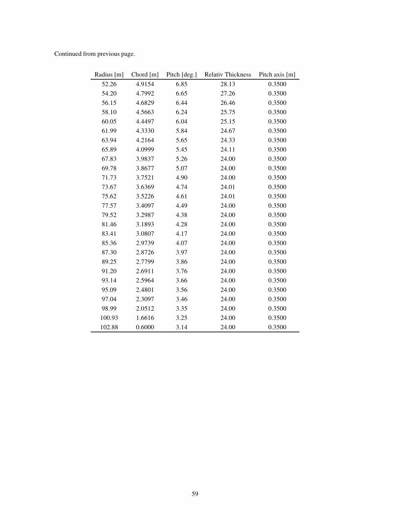
Continued from previous page.
Radius [m] Chord [m] Pitch [deg.] Relativ Thickness Pitch axis [m]
52.26 4.9154 6.85 28.13 0.3500
54.20 4.7992 6.65 27.26 0.3500
56.15 4.6829 6.44 26.46 0.3500
58.10 4.5663 6.24 25.75 0.3500
60.05 4.4497 6.04 25.15 0.3500
61.99 4.3330 5.84 24.67 0.3500
63.94 4.2164 5.65 24.33 0.3500
65.89 4.0999 5.45 24.11 0.3500
67.83 3.9837 5.26 24.00 0.3500
69.78 3.8677 5.07 24.00 0.3500
71.73 3.7521 4.90 24.00 0.3500
73.67 3.6369 4.74 24.01 0.3500
75.62 3.5226 4.61 24.01 0.3500
77.57 3.4097 4.49 24.00 0.3500
79.52 3.2987 4.38 24.00 0.3500
81.46 3.1893 4.28 24.00 0.3500
83.41 3.0807 4.17 24.00 0.3500
85.36 2.9739 4.07 24.00 0.3500
87.30 2.8726 3.97 24.00 0.3500
89.25 2.7799 3.86 24.00 0.3500
91.20 2.6911 3.76 24.00 0.3500
93.14 2.5964 3.66 24.00 0.3500
95.09 2.4801 3.56 24.00 0.3500
97.04 2.3097 3.46 24.00 0.3500
98.99 2.0512 3.35 24.00 0.3500
100.93 1.6616 3.25 24.00 0.3500
102.88 0.6000 3.14 24.00 0.3500
59


