D I - DTIC · Acknowledgements My sincerest gratitude is extended to my thesis advisor, David S....

AD-A258 VIENTATION PAGE om Approved

estimated to averaqe Inour pe '•esonse. I•nluding the time for reviewing rstructir•. seaf(rchng eisting data surces.9 arnd rev .rrf4 the ,'!-ecton Of rrtormatlon Sena comments regarding this burden estimate or any otrer asoecl of this9 th.3 o.roeri, to ,va,•hingto Headquarter, Serv :es. Directorate for rpformation Operations and Reports. 12 1 sJ-tfers•)

U,5'$ a IIinwv .s u ... .. , .*. . •... ...... to theO Of Ofie oM hianiagerent and buOciet. Paperwork RedumeJ r Prt'ject (0704.0188). Washifgt~n. 'DC 20503

1. AGENCY USE ONLY (Leave blank) 2. REPORT DATE .3. REPORT TYPE AND DATES COVERED

I May 14, 1992 THESIS/NJ X2. XA4. TITLE AND SUBTITLE S. FUNDING NUMBERS

Structural Simulation Coupling For Transient Analysis

6. AUTHOR(S)

Howard Travis Clark, III, 2nd Lt

7. PERFORMING ORGANIZATION NAME(S) AND ADDRESS(ES) 8. PERFORMING ORGANIZATIONREPORT NUMBER

AFIT Student Attending: Massachusetts Institute of AFIT/CI/CIA- 92-101Technology

9. SPON•ORING!MONITORING AGENCY NAME(S) AND ADDRESS(ES) 10. SPONSORING/MONITORINGAGENCY REPORT NUMBER

AFIT/CI

Wright-Patterson AFB OH 45433-6583

l1. SUPPLEMENTARY NOTES

"1"2a. DISTRIBUTION!/AVAILABILITY STATEMENT 12b. DISTRIBUTION CODE

Approved for Public Release lAW 190-1 WDIC (7'•7' !.. TTT--.,T-ft id

Distributed UnlimitedERNEST A. HAYGOOD, Captain, USAF Accesi n ForExecutive Officer

13. ABSTRACT (Maximum 200 words) E)Unannounced 0

JustificationD "I ¶ ................ .......................F-- ELE rTE By

• •E.C1O •°9 l Distribution/Availability Codes

Dist Avail and /or-. D.st Special

92-31211 7•!92 12 0 9 037

14. SUBJECT TERMS 15. NUMBER OF PAGES

16316. PRICE CODE

17. SECURITY CLASSIFICATION 18. SECURITY CLASSIFICATION 19. SECURITY CLASSIFICATION 20. LIMITATION OF ABSTRACT

OF REPORT OF THIS PAGE OF ABSTRACT

SS N, 7540-01-280-5500 Stindard Form 298 (Rev 2-89)

STRUCTURAL SIMULATION COUPLING

FOR TRANSIENT ANALYSIS

by

Howard Travis Clark, III

B.S., United States Air Force AcademyColorado Springs, Colorado (1990)

Submitted to the Department of Aeronautics and Astronauticsin Partial Fulfillment of the Requirements for the Degree of

MASTER OF SCIENCE

at the

MASSACHUSETTS INSTITUTE OF TECHNOLOGY

June 1992

© Howard T. Clark, III 1992, All Rights Reserved

The author hereby grants to M.I.T. permission to reproduce andto distribute copies of this thesis document in whole or in part.

Signature of Author_Department of Aeronautics and Astronautics

7 May 1992

Approved byDr. David S. Kang

Technical Staff, Charles Stark Draper LaboratoryThesis Supervisor

Certified byProfessor John Dugundji

Department of Aeronautics and AstronauticsThesis Supervisor

Accepted byProfessor Harold Y. Wachman

Chairman, Department Graduate CommitteeDepartment of Aeronautics and Astronautics

STRUCTURAL SIMULATION COUPLING

FOR TRANSIENT ANALYSIS

by

HOWARD TRAVIS CLARK, III

Submitted to the Department of Aeronauticaland Astronautical Engineering

on May 14, 1992in partial fulfillment of the requirements for the degree of

Master of Science

ABSTRACT

Analysis of the transient time response of many modern engineering

systems requires simulation by means of direct time integration of sets of

coupled-field equations. In the past the simulation of such coupled

problems has created difficulties which are not seen in analogous single-

field problems. Perhaps the most important of these difficulties is the fact

that existing engineering analysis packages have been oriented to solving

only single-field problems. This suggests one particularly attractive

option: the use of existing single-field analysis software while imposing

certain modular requirements. If modularity can be maintained, direct

integration of the equations can proceed by sequential or parallel

operation of the separate analyzers.

This research develops the theory by which the numerical

simulations of two or more separate fields may be combined to solve the

coupled-field problem. This theory allows simulations to be used with

little or no change by considering the constraints that provide for field

3

coupling. The development takes into account the various numerical

methods which may be used by individual simulations to solve their

separate problems. Above all this paper does not seek to suggest that

simulation coupling is the best or foremost simulation methodology

available, merely that it is a viable and cost saving alternative to solving

the larger, more involved coupled-field problem.

The specific discipline of focus will be multibody dynamics. The goal

will be to show that it is poxssible to couple multiple single body dynamic

analysis packages and come up with solutions comparable to the full

multibody dynamic case. The advantages of such a methodology are

readily seen here. The single body equations of motion are fairly simple

and a great deal of software exists to produce transient analyses of such

bodies. This is compared to the multibody analysis where the equations of

motion are not readily derived, few reliable analyzers exist, and changes in

the model may require a great deal of change to the analysis package.

The paper is organized into three main sections. The first section

deals with the tools necessary to evaluate the simulation coupling method.

The second part introduces this method as well as dealing with stability

and accuracy of the algorithm presented. The final section of the paper

involves numerical examples which demonstrate the strengths and

weaknesses of this theory.

Thesis Supervisor: Dr. David S. KangTechnical Staff, Charles Stark Draper Laboratory

4

Acknowledgements

My sincerest gratitude is extended to my thesis advisor, David

S. Kang, for his funding of this thesis and his all his help.

I would like to thank all those who have helped me during my

time at MIT and Draper, especially Dr. Dugundji.

I would also like to extend a special thanks to my friends at

Draper. Their help and friendship got me through many long days

and late nights and made sure the deadlines were met. Joe, Dave,

Mike, Ashok, Lou, Bill, and Kevin, thank you all and best of luck. I

also want to thank my roommate, Matt, who constantly reminded me

how much simpler life would be, if I only had a brain.

It is with all my love and appreciation that I thank my parents

for their love and support and without whom I would have never

made it this far.

5

This thesis was researched and written at the Charles Stark

Draper Laboratory under Internal Research & Development 332.

Publication of this thesis does not constitute approval by the

laboratory of the findings or conclusions herein, but is done for the

exchange and stimulation of ideas.

I hereby assign my copyright of this thesis to the Charles Stark

Draper Laboratory, Inc., of Cambridge, Massachusetts.

Howard T. Clark, III

2Lt., USAF

Permission is hereby granted by the Charles Stark Draper

Laboratory, Inc. to the Massachusetts Institute of Technology to

reproduce and to distribute copies of this thesis document in whole

or in part.

6

Table of Contents

A bstract ..................................................................................................................... 3

A cknow ledgem ents .......................................................................................... 5

Table of Contents ............................................................................................ 7

List of Illustrations ..................................................................................... 11

List of Tables .................................................................................................... 13

N om enclature .................................................................................................. 15

Chapter O ne Introduction .................................................................. 1 9

1.1 Background ....................................................................................... 19

1.2 M otivation for Current W ork ................................................... 20

1.3 Restrictions Considered ............................................................... 2 1

1.4 Overview .......................................................................................... 22

Chapter Two Solution Methods ofC oupled Field Problem s ............................... 25

2.1 Idealization of the Coupled-Field Problem .......................... 26

2.2 Field Elim ination ............................................................................. 28

2.3 Sim ultaneous Solutions ............................................................... 30

2.4 Partitioned Solutions .................................................................... 31

2.5 Simulation Coupling ....................................................................... 34

7

Chapter Three Methods for the Analysisof Numerical Integration ............................. 37

3.1 Time Discretization ....................................................................... 373.2 Effects of Computer Implementation ..................................... 41

3.2.1 Computing the Historical Vector ............................. 413.2.2 Choice of Auxiliary Vector ......................................... 42

3.3 Operational Notation ..................................................................... 443.3.1 The Shift Operator and the Z Transform ............... 443.3.2 Notation for Approximations and HistoricalV ectors ............................................................................................. 4 53.3.3 Notation for Forcing Term b, ................................... 47

3.4 Use Of Predictors .......................................................................... 483.5 E xam ples .......................................................................................... 4 9

3.5.1 Trapezoidal Rule ............................................................. 493.5.2 Gear's Two Step Method ............................................ 49

Chapter Four Constraint Equations andNumerical Simulation Coupling ............... 51

4.1 Methods of Handling Constraints ............................................. 514.1.1 The Lagrange Multiplier Method ............................ 524.1.2 The Penalty Method ..................................................... 55

4.2 The Simulation Coupling Process ............................................. 574.2.1 Concurrent Evaluation Coupling ............................. 604.2.2 Staggered Evaluation Coupling .................................. 62

4.3 Analysis of the Simulation Coupling Process ...................... 644.3.1 Stability Analysis of Simulation Coupling ........... 644.3.2 Accuracy Analysis of Simulation Coupling .......... 66

Chapter Five Illustrative Numerical Examples ................... 69

5.1 One Dimensional, Rigid Body Example ................................... 705.1.1 Analysis of 1-D Example ............................................. 715.1.2 Response of l-D Example ........................................... 75

5.2 Shuttle-Satellite Example ............................................................ 805.2.1 Stability Analysis of Shuttle-Satellite .................... 815.2.2 Accuracy Analysis of Shuttle-Satellite ................. 835.2.3 Response of Shuttle-Satellite Example .................. 86

8

5.3 Free Floating Rigid Body Example .......................................... 915.3.1 Analysis of Rigid Body Example

Translational DOFs ......................................................... 9 15.3.2 Analysis of Rigid Body Example

Rotational DOFs ............................................................... 935.3.3 Response of Rigid Body Example .............................. 96

5.4 Conclusions From Simple Examples ....................................... 98

Chapter Six Space Station Example ............................................... 101

6.1 Analysis for the Space Station Example ............................ 1026.2 Response for the Space Station Example ................................. 103

Chapter Seven Conclusion ........................................................................... 107

7.1 Sum m ary ............................................................................................... 10 77.2 Significant Findings and Results ............................................ 1087.3 Future W ork ........................................................................................ 10 9

Appendix A Satellite Rigid Body Plots ........................................ 111

A.1 First Case - Z Axis Forcing ............................................................. 111A.2 Second Case - Z Axis Torque ........................................................ 114

A.3 Third Case - Tri-Axis Forcing ...................................................... 117

A.4 Fourth Case - Non-Spin Axis Torque ........................................ 124

Appendix B Space Station Plots ....................................................... 137

B.1 Rigid Model Plots ............................................................................... 137

B.2 Flexible Model Plots .................................................................... 148

Appendix C Numerical Improvementsfor Simulation Coupling ............................... 155

C.1 Use of Rigid Body Predictors ..................................................... 155

C.2 Example of Rigid Body Prediction ........................................... 157

R efe re n c e s .............................................................................................................. 1 6 1

9

List of Illustrations

Figure Page

Figure 1.3-1 Coupled System Interaction ............................................... 22Figure 2.1-1 Arbitrary Two-Field Coupled Domain ........................... 26Figure 2.4-I Flow of Informatior in a Staggered Solution ............... 3 4Figure 5.2-1 Information Flow in Concurrent Evaluation ............... 5 8Figure 5.2-2 Information Flow in Staggered Evaluation ................... 5 9Figure 5.1-1 Satellite Rigid Body Model ................................................. 70Figure 5.1-2 Pole Locations of Rigid Body Model ................................. 74Figure 5.1-3 1-D Example Response to Constant Forcing .................. 76Figure 5.1-4 I-D Example Constraint Error, h = 0.008 ....................... 77Figure 5.1-5 I-D Example Response to Ramped Forcing ................... 78Figure 5.1-6 I-D Example Response to Pulsed Forcing ...................... 79Figure 5.2-1 I-D Shuttle-Satellite Model ................................................. 80Figure 5.2-2 Shuttle-Satellite Example Short Term Response ...... 87Figure 5.2-3 Shuttle-Satellite Example Short Term Error ............... 8 88Figure 5.2-4 Shuttle-Satellite Example Long Term Response ......... 8 9Figure 5.2-5 Shuttle-Satellite Example Long Term Error ...................... 9 CFigure 6.1-1 Space Station Freedom, Assembly Complete .................. 102Figure A.1-1 Translational Response for Case 1 ...................................... 112Figure A.1-2 Constraint Error Response for Case 1 ........................... 113Figure A.2-1 Rotational Response for Case 2 ...................................... 115Figure A.2-2 Constraint Error Response for Case 2 ........................... 116Figure A.3-1 Translational Rotor Response, Short Run, Case 3 ......... 118Figure A.3-2 Translational Platform Response, Short Run, Case 3..l 19Figure A.3-3 Translational Error Response, Short Run, Case 3 ..... 120Figure A.3-4 Translational Rotor Response, Long Run, Case 3 ....... 1 21Figure A.3-5 Translational Platform Response, Long Run, Case 3 ...122

11

Figure A.3-6 Translational E!Tor Response, Long Run, Case 3 ..... 123Figure A.4-1 Translational Rotor Response, Short Run, Case 4 ......... 125Figure A.4-2 Rotational Rotor Response, Short Run, Case 4 ............ 126Figure A.4-3 Translational Platform Response, Short Run, Case 4..127Figure A.4-4 Rotational Platform Response, Short Run, Case 4 ....... 128Figure A.4-5 Translational Error Response, Short Run, Case 4 ..... 12()Figure A.4-6 Rotational Error Response, Short Run, Case 4 ........... 130Figure A.4-7 Translational Rotor Response, Long Run, Case 4 ....... 131Figure A.4-8 Rotational Rotor Response, Long Run, Case 4 ............. 132Figure A.4-9 Translational Platform Response, Long Run, Case 4... 133Figure A.4-10 Rotational Platform Response, Long Run, Case 4 ....... 134Figure A.4-11 Translational Error Response, Long Run, Case 4 ........ 135Figure A.4-12 Rotaticnal Error Response, Long Run, Case 4 ...... 136Figure B.1-1 Z Force Response for Rigid Nonarticulated Case ..... 138Figure B.1-2 Z Force Response for Rigid Nonarticulated Case ..... 139Figure B.1-3 X Torque Response for Rigid Nonarticulated Case ........ 140Figure B.1-4 X Torque Response for Rigid Nonarticulated Case ........ 141Figure B.1-5 Z Force Response for Rigid Articulated Case ................... 142Figure B.1-6 Z Force Response for Rigid Articulated Case .............. 143Figure B.1-7 X Torque Response for Rigid Articulated Case ........... 144Figure B.1-8 X Torque Response for Rigid Articulated Case ............... 145Figure B. 1-9 Translation Errors for Rigid Nonarticulated Case ......... 146Figure B.1-10 Rotation Errors for Rigid Nonarticulated Case ............. 147Figure B.2-1 Z Force Response for Flexible Articulated Case ........ 149Figure B.2-2 Z Force Response f-'r Flexible Articulated Case ........ 150Figure B.2-3 X Torque Response for Flexible Articulated Case ......... 151Figure B.2-4 X Torque Response for Flexible Articulated Case ......... 152Figure B.2-5 Translation Errors for Flexible Nonarticulated Case .... 153Figure B.2-6 Rotation Errors for Rigid Nonarticulated Case ............ 154Figure C.l-l Two Field Rigid Body ............................................................ 156Figure C. 1-2 Force Balance Using Rigid Body Prediction .................. 157Figure C.2-1 Z Force Response for Rigid Articulated Case ............. 159Figure C.2-2 Z Force Response for Rigid Articulated Case ............ 160

12

m nm m i • m mm sal n f IIIIIIIIIII I~nlm~l• •

List of Tables

Table Page

Table 3.2-1 Steps in Finding hn .................................................................. 43Table 3.2-2 Remaining Steps in Finding Un ........................................... 43Table 3.3-1 Operational Constants in bn ................................................. 48Table 4.2-1 implementation of Concurrent Simulation Coupling ...... 62Table 4.2-2 Implementation of Staggered Simulation Coupling ......... 64Table 5.2-1 Comparison of Frequency Shifting Effects ...................... 85

13

Nomenclature

In general boldface text indicates vector or matrix quantities withupper case for matrices and lower case for vectors. Also, numbers inparenthesis represent the chapter in which a symbol occurs.

= d t first time derivative

C) = d2 second time derivativedt

2

= first variation operator (4)

det = determinant operator0 = zero matrix (of appropriate dimensions)I - identity matrix (of appropriate dimensions)

x,y = physical single field response variablesM = general mass matrix

C = general damping matrixK = general stiffness matrixR = general nodal forcing functions

or nonconservative external factors in Lagrange'sequations of motion

( = physical constraint and interface condition equations

fc = effective constraint forcesu = coupled field response variables = Laplace variable

v = auxiliary vector in order reductionA,B = weighting matrices in choice of v

w general vector for integrationh = integration stepsize

15

i, = constants for integration approximationhnw = collection of historical terms associated with w

pertaining to time t = tn

ho 0, effective stepsize (3)

70 = constants for second order integration approximationAn,bn = complex matrix and forcing function for integration (3)

= shift operatorz = discrete variable, z = esh

= operator notation polynomials

4' = operators constants in forcing term b .p = operator notation associated with predictors

T = kinetic energyV = potential energyF = Rayleigh's dissipation function

A = action integralL = Lagrange's function, Lagrangian

= Lagrange multiplier

G = •-, Jacobian of constraints wrt u

K, = constants in penalty method

H = -, Jacobian of constraints wrt u

S = complex polynomial for prediction of constraints

C = system characteristic equation/matrixR = translation from inertial (5)

0 = Euler angle rotationsa Cb = rotation matrix from frame b to frame a

CO = angular momentum of a bodyS = transformation from Euler angle rates to angular

momentum coordinates

16

Subscripts

x or y = attendant matrix of single field analysisxx,yy,

xy,yx = attendant matrix of couple field analysish or nh = indicates with holonomic or nonholonomic problems

r, p = indicates rotor or platform(5)a, s = indicates arm end effector or shuttle(5)

ss = indicates steady state quantity0 = indicates inertial quantity

Superscripts

T = transpose operatorI = implicit portion of a partitionE = explicit portion of a partitionc attendant matrix connected with constraints

u, v, w = denotes quantities associated with integration vectorsU, V, or W

P = terms are associated with prediction (3,4)= indicates a normalized quantities (3)

indicates concurrent or staggered coupling (4)* = fictitious qualifier (ie. V* = fictitious potential energy)

Acronyms

IE = implicit-explicit (partitioning scheme)IXF = degrees-of-freedomCM = center of mass

17

Chapter One

Introduction

1.1 Background

Flexible multibody problems have become increasingly

important in recent years, primarily to support the design and

deployment of large space structures. The numerical simulation of

these problems becomes especially important in space applications

where extensive laboratory research is impractical. Flexible

multibody dynamics, however, is only a subset of the larger group of

coupled-field problems whose numerical solution has been the

subject of a great deal of study over the past decade. Coupled-field

systems are readily solved single-field subsystems linked together

by constraints or interface boundaries; systems whose solution is

made difficult by the size of the combined problems, the widely

varying time response characteristics that the combined subsystems

may have, and the fact that most analysis software currently

available is written for single-field analysis.

Traditional solutions to the coupled-field problem involve

solving the system as a whole, either through field elimination or by

19

STRUCTURAL SIMULATION COUPLING FOR TRANSIENT ANALYSIS

simultaneous solution. Recently, partitioned solution methods have

received a great deal consideration for their ability to divide the

problem into pieces which may be dealt with individually. A more

extreme form of partitioning exists in the form of simulation

coupling, where the constraint or boundary interface effects are

combined with single field analyzers to solve coupled systems.

The major advantage of the simulation coupling method is its

maximal use of available software and existing analyses. This is

especially true for coupled structural problems. Transient analysis of

such problems are of particuiar interest in the design process when

variations of secondary structural systems need to be coupled to a

primary structure. Analysis of the loading due to different satellites

carried in the space shuttle's main bay and the construction and

deployment of laboratory and habitation modules connected to the

space station's main structure are two examples where, if certain

stability and accuracy needs can be reached, there would be an

advantage to coupling existing simulations instead of using the more

traditional methods to re-solve the problem for each variation.

1.2 Motivation for Current Work

Analysis of the transient time response of many modern

engineering systems requires simulation by means of direct time

integration of sets of coup!ed-field equations. The simulation of such

coupled problems has created difficulties which are not normally

seen in analogous single-field problems. Perhaps the most important

of these difficulties is the fact that existing engineering analysis

20

HAIE ONEI IRODUCTION

packages have been oriented to solving single-field problems. This

suggests one particularly attractive answer: the use existing single-

field analysis software while imposing certain modular requirements.

If modularity can be maintained, direct integration of the equations

can proceed by sequential or parallel operation of separate analyzers.

The motivation for this thesis is the development of a theory

by which the numerical simulations of two or more separate fields

may be combined to solve the coupled-field problem. This theory

should allow simulations to be used without change through

consideration of the constraints that provide for the field coupling.

This theory should account for the various numerical methods which

may be used by the individual simulations to solve their separate

problems. It should be noted that this thesis is aimed at solving

coupled problems where at least one field is structural in nature.

Even then the arguments and theory contained within this thesis are

aimed at the more physical interaction problems (ie. fluid-structure

and structure-structure problems versus control-structure and

thermal-mechanical problems).

1.3 Restrictions Considered

In developing the theory described earlier certain restrictions

of the general problem are assumed. First, the constraints which

couple the separate fields are assumed to exist as two-way

interactions between two individual fields. For this reason the

coupled problem can be examined by considering only two fields.

21


Additional fields can be dealt with in a similar fashion. Figure 1.3-1

shows the allowable interactions for a system of three coupled fields.

Separate Fields

Two-Way Constraints

Figure 1.3-1 Coupled System Interaction

It is also assumed that the equations of motion for the separate

fields are initially describable in a semi-discrete second order form:

Mi + Ci + Kx = R(t)

This is not an overly limiting assumption since most fields in coupled

problems are easily placed in this form.

1.4 Overview

The remainder of this thesis is organized in the following

manner. Chapter two reviews the available methods of solving

coupled field problems along with the benefits and shortcomings of

each method. Field-elimination and simultaneous solutions are

discussed as well as partitioned solution methods, where simulation

coupling is introduced as a special case of these methods.

22

CHAPTER ONE: INTRODUCTION

Chapter Three describes some of the tools essential to the

development of the theory for coupling simulations, namely

integration procedures and stability analysis procedures.

Chapter Four sets forth the simulation coupling procedures in

addition to discussing how to deal with the constraints which couple

the separate fields. The stability and accuracy of the coupling

procedures are also discussed.

Chapters Five and Six set forth numerical examples designed to

illuminate points made about the simulation coupling theory

developed in chapter five. Chapter Five involves small scale

examples designed to highlight specifics on the stability and accuracy

of this method. Chapter Six is dedicated to the large scale example,

namely, coupling single body simulations to form the assembly

complete form of the space station; a problem at the scale to which

simulation coupling is specifically directed.

Chapter Seven concludes this thesis by reviewing work done,

major findings included within, as well as outlining future work for

consideration in this area.

23


24

Chapter Two

Solution Methods ofCoupled-Field Problems

This chapter presents a basic overview of the primary means

by which coupled-field problems are solved. These problems are

often sufficiently large and complex that the only feasible solution

process is direct integration, which leaves the major question of what

form to place the equations of motion in order to carry out the

integration. Field elimination and simultaneous solution are standard

methods by which these problems are currently handled although

both have serious drawbacks which hinder their performance. More

recently partitioned solutions have been suggested as a possible

alternative [2.1-2.10]. A large number of partitioning schemes have

been recommended in literature and some of the more popular

methods will be introduced here. At the end of this chapter

simulation coupling is shown as a natural extension of partitioned

solutions.

25


2.1 Idealization of the Coupled-Field Problem

Consider an arbitrary domain, S, shown in Figure 2.1-1.

Allowing that S is the domain of a two-field coupled problem it may

be decomposed into three distinct subdomains: Sx and Sy, the

separate single field subdomains; and S1, the interface subdomain.

Sx

Figure 2.1-1 Arbitrary Two-Field Coupled Domain

If the effects of SI are ignored then the single fields may be

modelled by finite difference or finite element methods as

semidiscrete, linear, second order matrix differential equations

MxiE + CXx + Kxx = R,

Myy + Cy + Kyy = Ry (2.1-1)

where

x = x(t),y = y(t) : Separate field response vectors

M X, My General mass matrix

C X, Cy : General damping matrix

Kx, Ky General stiffness matrix

26

CHAPTFM TWO: SOLUTION METHODS OF COUPLED-FIELD PROBLEMS

Rx= Rx(t),Ry = Ry(t) : Separate field vector forcing functions

and ' ) denotes time integration

The fields expressed in equation (2.1-1) are coupled by the physical

constraints and interface conditions of S, which are expressed as

cI•(x,,,x,y) = 0 (2.1-2)

Note that the constraints which lead to coupled-field problems are

generally not assumed to be time varying functions.

Through appropriate use of Lagrange multipliers, penalty

formulations, or other methods equations (2.1-1) and (2.1-2) may be

combined as

Mxi + CXX + Kxx = Rx + fcx

Myy + Cyy + Kyy = Ry + fcy (2.1-3)

where fcx and fcy are effective constraint forces used to correct the

separate field response.

In the case where the interactions are linear in nature then

(2.1-3) can be rearranged as follows:

MxXi + CxxX + Kxxx =Rx - CxyY -KxY

Myyy" + Cyyy• + Kyyy =Ry - Cyxi Kyxx (2.1-4)

or if u = [XT yT ]T

Mii + Cu + Ku = R (2.1-5)

where

27


M = MXX0 Y] C Cxx Cx 1, K [Kxx Ky]0 MY Cyx Cyy Kyx Kyy

and R =[RT RyTr]T

Note: Kx may be modified by terms from fcx in (2.1-3) in order to

obtain Kxx in (2.1-4). Similar effects may be seen in Kyy, Cx,, Cyy.

However, M xx = M x and M yy = M y.

2.2 Field Elimination

Field elimination is aimed at the elimination of the interaction

terms through substitutions from the other available equations. This

method is usually suggested when the response of one field is

considered to be more important than the other. This process

reduces the number of states associated with each problem to only

one field but has several considerable drawbacks which should be

highlighted in the following example.

Consider the simpler system of the form of (2.1-4)

Mxxi + Cxxi + Kxxx = Rx - KxyY

Myyj + Cyyy + Kyyy = Ry - Kyxx (2.2-1)

Transforming these equations by means of the Laplace variable

(Mxxs2 + Cxxs + Kxx)X(s) = Rx(s) - KxyY(s)

(Myys2 + Cyys + Kyy)Y(s) = Ry(s) - KyxX(s) (2.2-2)

Eliminating Y(s) from (2.2-2a) using (2.2-2b)

28

CHAPTER TWO: SOLUTION METHODS OF COUPLED-FIELD PROBLEMS

[(MyyS2 + Cyys + Kyy)Kxy'l(Mxxs2 + Cxxs + Kxj)- Ky ]X(s)=(Myys2 + Cyys + KyyxyRx(s) - Ry(s) (2.2-3)

Multiplying through

{(MyyKxy-1Mxx)lS + (CyyKxylMxx + MyyKxylCxx) s3

+ (MyyKxy-'Kxx + CYYKxy'lCxx + KyyKxylMxxs2

++(KyyKxy-Cxx+CyyKxy-Kxx)s +(KyyKxy- x Kx}yx }X(s) (2.2-4)

= (Myys2 + Cyys + Kyy Kxy'Rx(s)- Ry(s)

Use of the inverse Laplace transform returns a differential

expression

(MyyKxy'IM xxl'X" + (CYYKxy-'Mxx + MyyKxy'lCxx)'X

+ (MyyKxylKxx + CYYKxy-'Cxx + KYYKxylMxx)

+ (KyyKxyXCxx + CYYKxY'Kxx)X I+ (KYYKxyXKxx - Kyx)X (2.2-5)

= MyyKxy'lix + CYYKxyYXRx + KYYKxy-'Rx - Ry

An expression similar to (2.2-4) can be found for the variable y(t).

The following disadvantages can be seen in this example:

- Higher-order derivatives are introduced for which there are no

readily available integrators.

- Additional initial conditions are required.

- Additional derivatives of the forcing functions are required.

- The sparsity (and possibly symmetry) of the attendant matrices is

lost.

- There is little possible use of existing software or single field

analyzers

29


- The above disadvantages become more serious as the complexity

of the problem increases.

Although field climination does succeed in reducing the states

associated with the problem it does so at the cost of introducing

further difficulties not easily solved at this time. Furthermore, every

time a secondary field to be coupled with the primary changes the

process must be repeated to solve the new problem.

2.3 Simultaneous Solutions

In simultaneous solution methods the coupled equations of

motion are integrated as a single large second-order problem in the

form of equation (2.1-5). By integrating all the equations in second-

order form, as opposed to field elimination procedures, higher order

derivatives and additional initial conditions are not required. In

addition there are accepted integration methods for use on second-

order differential systems. However, to be placed in the form of

(2.1-5) the interactions must be linear and there is still no possibility

of using existing single field analyzers.

Another shortcoming of this method is the requirement of

treatment in fully explicit or fully implicit form. This specification

carries with it the following problems. Since coupled problems

typically have very diverse time characteristics, the stability limits

on the step size tend to be unreasonably restrictive. This is

especially true if the problem includes rigid effects or incorporates

the constraints by penalty formulations. Also the interaction tends

30

CHAflER IWO: SOLUTION METHODS OF COUPLED-FILD PROBLEMS

to produce extremely large bandwidths in the associated coefficient

matrices. As a result the solution of realistic three dimensional

problems becomes rapidly prohibitive due to the number of

calculations necessary to set up and solve equations involving these

matrices.

So despite the superiority of simultaneous solutions to field

elimination there still exists the problem of setting up and solving

large set of coupled equations, along with a continued lack of

modularity.

2.4 Partitioned Solutions

Partitioned solution methods are based on dividing the system

matrices of equation (2.1-5) into two parts,

K=KI+KE and C=CI+CE (2.4-1)

where K' and C' are the inilicit portions of the partition and KE and

CE are the explicit portions. It should be mentioned that the entire

mass matrix must be contained in the implicit portion of the partition

(see [2.6]). In a partitioned solution the explicit portion, combined

with a predictor, acts like an applied force input to the differential

equation. There are two things which define a partition method: the

partitioning strategy and the particular partition used to divide the

system matrices.

The partitioning strategy is defined by the point at which the

partitioning occurs. At some point in order to solve the differential

system a numerical integration scheme must be applied. If the

31


scheme is applied and then the resulting matrix equation is

partitioned the strategy is call algebraic partitioning. If the partition

is applied before the integration scheme, then a differential

partitioning strategy results. The work of Felippa and Park [2.6]

shows a strong connection between the stability of the method and

the partitioning strategy used.

For a two-field system there are sixteen possible ways to fully

partition the system matrices and six of these simply represent field

switches. The ten remaining unique partitions for the explicit

portion, KE are

1[o 01] 2[ 0 0]1[ 10 0 ] 4[0x 01]5[ 0 K 12.-20 0 0 Ky Ky 0 8 y Ky1 0 Kyyl(2.4-2)

6 [ Kxx 0 70 7 8[Kx Kxy Kx 1Kj ~

0 Kyy Kyx 0 1 0 Kyx Kyy Kyx Kyy

The first and last cases correspond to the limiting fully implicit and

fully explicit simultaneous solutions, respectively. Partitions

numbers 2, 4, 5, 8, and 9 are all implicit-explicit partitions with 2

and 4 being more widely used, as will be discussed later. Also

number 3 is of particular importance; it is referred to as a staggered

partition and warrants further consideration. A more complete

analysis of all the available partitions is contained in [2.7].

Implicit-explicit partitions were first suggested for use in

structural dynamics by Belytschko and Mullen [2.1,2.2] in problems

where the mesh had two distinct set of time characteristics. The

specific application in mind were fluid-structure problems where a

very large, slow responding mesh (fluid) was coupled with a smaller,

32

CHAPTER TWO: SOLUTION METHODS OF COUPLED-FMELD PROBLEMS

quicker responding mesh (structure). Since the fluid mesh is very

large an explicit method was desired for improved computational

efficiency, but the large range of response frequencies in the

structure called for an implicit method for stability. By introducing a

boundary field, thus making it a three-field problem, and a three-

field partition equivalent to 4 the fluid was dealt with explicitly and

the structure implicitly. This form of partition is known as node-by-

node implicit-explicit (IE) partitioning.

Shortly thereafter Hughes and Liu [2.3,2.4] introduced the

three-field partition based on 2. This model defined the elements as

either implicit or explicit. The element-by-element IE partitioning is

easier to implement but may be more computationally intensive for

large boundary problems. However both element-by-element and

node-by-node IE partitioning still retain little modularity in solving

the problem.

Perhaps the most extensively used partition is the staggered

partition. It has thus far been effectively applied to fluid-structure

interaction problems [2.10], control-structure interaction problems

[2.9] and multibody dynamic simulation [2.8]. Staggered solutions

predict one field (in this case x) and use the prediction to solve the

second field (y). The first tield is then solved using the solution of the

second in an implicit fashion. This process is depicted below in

Figure 2.4-1 where EP is an explicit prediction flow and IS is an

implicit solution flow. Although it has been successful in allowing

more use of single field analysis software [see 2.6], it still does not

come through with the desired modularity.

33


Field X• Field YTime t

is EP is

l X Time t+dt

Figure 2.4-1 Flow of Information in a Staggered Solution

2.5 Simulation Coupling

Simulation coupling does not fall under one of the ten

partitions already mentioned since it is not a complete partition.

Instead of starting from (2.1-5) the partition is formed from the

terms in (2.1-3)

Mxx + Cxi + Kxx = Rx + fox

MyY + Cyj + Kyy = Ry + fcy

If these equations are manipulated into the form of (2.1-5) they look

like

0 M] 0 Cy 0 Ky fc y (2.5-1)

where all terms are as previously defined.

Again by approximating the interaction terms as linear, the

effective constraint terms may be written

34

CHAFlER TWO: SOLUTION MENHODS OF COUPLED-FIELD PROBLEMS

J CY CFYY I Kcyx KryJ (2.5-2)

Using these terms the partition for simulation coupling is

defined as follows:

K- Kx Jand KE = I X J (2.5-3)0 Ky KIy KY yyI

and the damping terms are similarly partitioned. The advantages to

using such a partition are that the implicit portion of the partition is

exactly the single field problem with interaction effects neglected.

This is readily seen by examining the left-hand side of (2.5-1), where

the system matrices are completely uncoupled. The interaction

effects are handled exclusively in the explicit portion of the partition.

This solution form allows existing single field analysis packages to be

applied directly with the inclusion of constraint terms as applied

forces being the only modification necessary. As this is a partitioned

solution form, the partitioning strategy, the chosen predictors, as well

as the details of implementation have great impact on overall

stability and performance of simulation coupling. These effects are

addressed in the remaining parts of this thesis.

35


36

Chapter Three

Methods for the Analysis ofNumerical Integration

Since the primary means of solving large sets of differential

equations is direct time integration, it is important to review the

basic theory and notation involved. This chapter outlines reduced

order forms as well as operational notation used to determine the

stability of a given procedure. Additionally, details of computer

implementation such as computational paths and choice of auxiliary

vectors are covered. Much of this information was first introduced

by Jensen [3.1] and is covered in detail in a series of papers by

Felippa and Park [3.2, 3.3 and 2.6].

3.1 Time Discretization

The equation for a general space-discretized structural system

described earlier is

Mii + Cu + Ku=R (3.1-1)

37


This system may be placed in reduced first order form by

introducing an auxiliary vector, v (see [3.11)

v = AM6 + Bu (3.1-2)

where A and B are suitably chosen n x n matrices. By manipulating

(3.1-1) ii may be eliminated in favor of v

AMu +ACu +AKu=AR -* ,+(AC -Bhi+AKu=AR(3.1-3)

With the equations of motion cast in first order form [(3.1-2) and

(3.1-3)], numerical integration is carried out by introducing a first

order, linear multistep integration approximation for the variables ui

and V*. Given a constant stepsize, h, the form of such approximations

is

m m

I aiwn-i = h 1 PiWn-ii=O i=O (3.1-4)

The ai's and Pi's are specific to each approximation and frequently

normalized so that a0 = 1. Also, w k is a generic vector with k

denoting the vector w(t) at time t = tk.

Note 1: A large number of integration methods have been left

out due to the restriction to linear multistep methods. Perhaps the

most frequently used of these are the Runge-Kutta class. Although

popular, this class is not feasible for large scale problems like

structural simulation due to their multiple derivative evaluations per

time step and the difficulty associated with analyzing the stability of

multiple evaluation methods.

38

CHAPFER THREE: METHODS FOR THE ANALYSIS OF NUMERICAL INTEGRATION

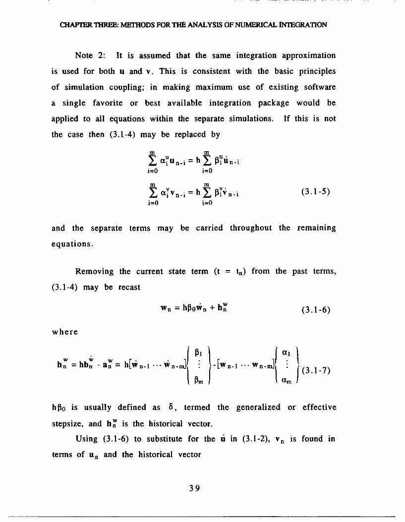
Note 2: It is assumed that the same integration approximation

is used for both u and v. This is consistent with the basic principles

of simulation coupling; in making maximum use of existing software

a single favorite or best available integration package would be

applied to all equations within the separate simulations. If this is not

the case then (3.1-4) may be replaced by

m mau u =h u"•i Uni = [i Un-i

i=O i=O

m m (.4Sa~v = h 0y. (3.1-5)Oi Vn-i =iVn-i

i=0 i=O

and the separate terms may be carried throughout the remaining

equations.

Removing the current state term (t = tn) from the past terms,

(3.1-4) may be recast

Wn = hipoWn + hw (3.1-6)

where

W W- r.W]hn =hbw an =hWn- .. Vin-n " -[Wn-1 ... Wn-h[ ,. .- (31 )

h 30 is usually defined as 8, termed the generalized or effective

stepsize, and hw' is the historical vector.

Using (3.1-6) to substitute for the ti in (3.1-2), vn is found in

terms of un and the historical vector

39


8Vn = (8B + AMýun - AM hun (3.1-8)

This equation can be used along with forms of (3.1-6) for u and V' to

remove everything except Un, the historical vectors hnu and hv', and

the current forcing term Rn from (3.1-3). Making the appropriate

substitutions leaves

[M• 8-C+B2Klun =[M• + 8(C - A'ln)]hu + 8iA'lhn + 52an (3.1-9)

Note 3: Until now nothing has been said about discretization by

means of the popular second order methods, such as Newmark,

Houbolt, or Wilson-0 integration. These second order, linear

multistep methods have been examined in detail by Geradin [3.41

and are easily cast in forms similar to the first order methods. Two

integration approximations are required, one like the first order (3.1-

4), the other in terms of accelerations

m mIauni = h 1 Piuin-i

i=0 i=O

IYiUni = h2 n1 Y Piin-i (3.1-10)

i=O i=O

or in simpler notation

Un = 8ulin + hu

Un = h iin + h(3.1-11)

where 8u is 8 from before, hu is as defined in (3.1-7) and hhn is

defined as

40

CHAPTER TREE: METHODS FOR THE ANALYSIS OF NUMERICAL INTEGRATION

h =h21jb 6 - cu = h2l,[ii n-1 -. iin. " -[Un.1 ... Un-m] i( .- 2

Using (3.1-11) to substitute for ii and ii in (3.1-1) and defining

= hrj results in a final form similar to (3.1-9)

[M + BuC + 8d~uK]un = Chu + M h + kSuRn (3.1-13)

Since this result is merely an extension of the first order form (by

choosing v = u and using separate integration formulas for each), it

may be treated in the same fashion and is not be dealt with

independently.

3.2 Effects of Computer Implementation

There are two primary decisions to be made when

implementing a numerical integration scheme. The first involves

choosing one of the equations already presented to compute the

necessary terms for h', while the second deals with the choice of

weighting matrices A and B to determine the auxiliary vector v.

Both decisions affect the solution's stability, error propagation, and

efficiency.

3.2.1 Computing the Historical Vector

The calculation of the historical vector h n is referred to as the

computational path. The three steps in finding h', for each of the

three paths (0,1,2), are shown in Table 3.2-1. The remaining steps

which find hu, form the right hand side of (3.1-9), and then solve for

41


u. are the same for all paths and are listed in Table 3.2-2. It should

be mentioned that there are other possible ways in which h' may be

calculated, but these are the most frequently encountered. However,

one common variation is to update 6. within the 0 path, creating a 0'

path.

3.2.2 Choice of Auxiliary Vector

There are two widely accepted choices for v. The physically

intuitive choice is to let v = u'. This is called the conventional form of

v. The other major form was introduced in [3.1] by Jensen. This form

is determined by

v = Mu, +Cu (3.2-1)

so that V = R-Ku. The conventional form and Jensen's form are

numerically equivalent, however, the effort and efficiency of each is

significantly different.

The conventional form has the benefit of reducing four state

vectors to three ([ u,i,v,, I to [ u,u,u 1) as well as the physical

significance of v. Unfortunately, this form sometimes requires a

non-singular mass matrix. Jensen's form does not have this difficulty

and is more computationally efficient than the conventional form

(see [3.2]). It should be noted, however, that in a simulation coupling

context the auxiliary vector and the computational path are

determined by the choice of integration package and not selected for

efficiency or effectiveness of implementation of the overall coupled

problem.

42

CHAPTER THREE: METHODS FOR THE ANALYSIS OF NUMERICAL IEGRATION

Table 3.2-1 Steps in Finding hv

Variable Equation Used Form of Equation

0 Path

Vn- 1 (3.1-3) Vn-1 +(AC - B)6n-1 + AKun. 1 - ARn-1v

Vn-1 (3.1-6) Vn-1 = hfpoi 1n-1 + hn-1v v

h_____ (3.1-7) hn = hb - an

1 Path

(3.1-3) i;n-I +(AC - B)fin-i1 + AKun-1 =ARn-1

vn-1 (3.1-2) Vn-x = A Muln- 1 + Bun-1v v

h___ (3.1-7) hn =hbn -an

2 Path

Vn-1 (3.1-2) Vn-1 = A Mun- 1 + Bun-1

Vn-. 1 (3.1-6) Vn-1 =(vn- 1 -hv-l)/hl3hV V317 v v

n_ (3.1-7) hn = hbI- an

Table 3.2-2 Remaining Steps in Finding Un

Variable Equation Used Form of EquationU U u

hn (3.1-7) hn = hbn- an

bn(3.1-9) [M + 8(C - A'B)]hu + 8A'lhv + 82Rn

An (3.1-9) [M + +82K]

Un Solve Anun = bn

in (3.1-6) in =(un-hU)/hn 0

43


3.3 Operational Notation

Operational notation is presented to produce a concise

presentable notation form and to facilitate stability and accuracy

analysis. The discrete Laplace transform and the z-transform are

introduced to the integration approximation and the historical terms

to produce an operational expression for b., the right hand side of

(3.1-9). All of these expressions are necessary for the evaluation of

the simulation coupling algorithm.

3.3.1 The Shift Operator and the Z Transform

In any series a single term may be related to the previous or

following term by means of the shift operator

wk wk-1-WWk= Wk Wk = Wk+1 (3.3-1)

Repeated application will relate any term W k to the initial or final

term

Wk= w0 , Wk Wn (3.3-2)

Since the integration methods discussed so far require only the

Wnn-m,...,Wn terms, we can focus on the second of each of the forms

above. Applying the discrete Laplace transform to the shift operator

produces

Wk = e(k'n)sh Wn (3.3-3)

Substituting the standard z-transform definition, z = esh, into the

44

CHAPTER THREE: METHODS FOR THE ANALYSIS OF NUMERICAL IN4EGRATION

above expression

Wk = Zk'n Wn (3.3-4)

With these definitions a function f

f(k) = Wn + ailwn_1 + a2Wn-2 + a3Wn.3 (3.3-5)

is transformed into the Laplace domain

f(s) = (1 + a1e'sh + a 2 e"2 sh + a 3e' 3 sh) wn (3.3-6)

and into the z domain

f(z) = (1 + alz'1 + x2Z'2 + a3Z'3 ) Wn (3.3-7)

or sometimes

f(z) = Z3(Z3 + a1Z2 + a 2Z1 + ax3) Wn (3.3-8)

Although for the function listed above the Laplace and z variables

are exact, the substitutions which following are only approximately

true. Since the time series is obtained from numerical integration

the properties of the shift operator in (3.3-1) and (3.3-2) are not met

exactly as they would be if the true solution series was used.

3.3.2 Notation for Approximations and Historical Vectors

Since numerical integration produces a time series of vectors

the terms may be readily carried into the Laplace or z domains.

Given an integration approximation of the form previously

introduced (where ao is normalized to 1 and now factoring 30o out,

leaving I3'i = Pi/130)

45


m ( m)

Wn + iWn-i Wn + i3n-i-9)i=l 1 339

Applying the shift operator and taking the discrete Laplace

transform of the approximation gives

1 + m ieish n=e1 + m j'e ni1 i(3.3-10)

or in the z domain1 _ Otz'i =• 1 + • 1'iZ~wi

1 i=l nI i n (3.3-11)

By rearranging (3.1-6) the historical vector may be written as

= W - (3.3-12)

Using this definition for hw, (3.3-10) and (3.3-11) may be

manipulated to form the following expressions:

h (s) = 8 e h " - (ie-'s)wnn (xe n

( P iz')1n - (z)iZ n (3.3-13)

It is useful to define commonly occurring polynomials in z and esh

m -

P(') + i()

i--1

a(.) = 1 + J I3'i(.) (3.3-14)i--1

Then in either domain

46

CHAPTER THREE: METHODS FOR THE ANALYSIS OF NUMERICAL INTEGRATION

P(.)Wn = 8(.)W n (3.3-15)

This also allows the historical vector to be written as

hn (0(.)- 1)n + (1P(.)) (3.3-16)

Another useful operator definition which is needed is

Wn = [p(.)/8&(.)] Wn = V(.)Wn (3.3-17)

3.3.3 Notation for Forcing Term bn

The presence of hn in the forcing term requires that

computational path be dealt with in order to come up with the

correct notation. Although each path has a distinct operational form,

the choice of auxiliary vector has no effect. Recalling the basic form

of bn

bn = [M + 8(C -A-IB)]hu + 8 + AR (3.3-18)

Using the definitions of the previous section hn can be written

hn(.) -8v(.)) (3.3-18)

which is also independent of path. The form of hn for each path

comes from the equations in Table 3.2-1 and when combined with

the above equations the following general form results:

bn = [ýMM + -C4+ KK] Un + tRRn (3.3-19)

These constants are detailed in Table 3.3-1.

47


Table 3.3-1 Operational Constants in b.

Path 44 0C 'K OR

0 1-o 0 82-1 8v"1

1 1 4.p2/Ca) 4(1-p) 82(l _0) 2(

2 1 _____ 1 (1-8V,) 0 1

3.4 Use Of Predictors

Simulation coupling is made possible by the ability to

accurately predict w. from earlier knowledge of w. A general linear

multistep predictor is suggested in [2.6] for use in large coupled

problems. The form of this predictor is

Wn M M P 0MP."= aiWn-i + hoo P [in'i + (h yiWn-ii=l i-- i=1~ Wf. (3.4-1)

As with the integration methods it is also beneficial to place the

predictor in operational form by defining polynomials in esh and z as

follows:m -i

Pw(.) = x tP.i=l

M P -

pi,(.) = 8 J•(.) (3.4-2)i=l1

2 m P

i=4

48

CHAPER THRE: METHODS FOR THE ANALYSIS OF NUMERICAL INTEGRATION

Using these definitions as well as (3.3-16) gives the final form of the

predictor as:

wn(.) = p(.)Wn = [Pw(.) + BNpiP(.) + (V) p•(.)Jn (3.4-3)

3.5 Examples

3.5.1 Trapezoidal Rule

The trapezoidal rule is a one step (m=l) implicit method

commonly used in many integration applications. Its constants are

ao = 1, al = -1, P0 = = 0.5

Then the operational forms are

p(esh )=1-esh,p(z) = 1 - z"

-shA -1O(esh) - + e' ,(z)= 1 + z

(esh) 2_ l sh tanh(s h / 2), V(z) = 2_ 1 - z1 2_ 7.

h 1 +e-sh h h 1+z-1 h z+l

and the historical forms are

hn (s)= (0.5 h in + wn)e sh

hn(z)= (0.5 h Vn + Wn)Z -

3.5.2 Gear's Two Step Method

Another implicit method introduced by Gear in [3.5] is a two

step A-stable form. Its constants are

ao = 1, al = -4/3, a2 = 1/3

00 = 2/3, 01 =P2 = 0

The operational forms are

49


p(esh) =) I - 4 -•' s + '"s, p(Z) = I - I +_ L--2

3 3 3 3

0(e =1 c=(z)

V(esh)= 2-3h-i 4e-sh + l- 2sh =3 - 4esh +e2sh3 3 2

v,(z) (3= I- z" I + =z' 3 _4z+-2h 3 32hz2

and the historical forms arehW(s) = 144 eSh e2sh)

3h nw5(z) = 0-4z'1 - z'2)

50

Chapter Four

Constraint Equations andNumerical Simulation Coupling

Before the simulation coupling process may be fully developed

and analyzed, the incorporation of constraints into equations of

motion must be covered. The remaining portion of this chapter

provides the details of simulation coupling. Finally, the analysis of

the stability and accuracy of the coupling process is addressed.

4.1 Methods of Handling Constraints

In an attempt to develop an accurate and reliable method of

dealing with constraints, many different procedures have been

suggested [4.1-4.61. Two methods of primary interest for use in

coupled-field problem are penalty formulations and more traditional

Lagrange multiplier forms. Besides the basic implementations of the

methods there are additional stabilization procedures to improve

performance which are covered. Both methods detailed here are

developed from using traditional variational principles and

specifically the Euler-Lagrange equations.

51


4.1.1 The Lagrange Multiplier Method

A typical n-DOF mechanical system is defined by the following

energy products:

Kinetic: T- 1-iTM Ui and Potential: V = LuTK u (4.1-1)

2 2

as well as

F=C 6 (4.1-2)

where F are Rayleigh's dissipative forces, representing damping

proportional to velocity. Additionally, the response of the system is

restricted by

4'(u,u,t) = 0 (4.1-3)

where 4 is a vector of p individual constraints.

When no derivative terms are present, these functions may be

used to eliminate p DOFs in the vector u. Unfortunately, this is can be

difficult and it is not always clear which individual degrees should be

removed. Instead, Lagrange's "method of the undetermined

multiplier" may be used to form a term which represents the forces

which ensure the constraint is satisfied. This term, along with the

nonconservative externally applied forces, BW = R~u, and energy

products, may be combined to form the action integral for a

constrained system

A 1 (L + W + Tx + pT u) dt (4.1-4)

52

CHAPTER FOUR: CONSTRAINT EQUATIONS & NUMERICAL SIMULATION COUPLING

where X is the vector of Lagrange multipliers and L is the Lagrangian

T - V. By applying the principle of least action, 8A = 0, the Lagrange

equation of motion is

-LaL - r - aDT (4.1-5)

By using (4.1-1,2) in (4.1-5) the matrix equation of motion for a

constrained system is obtained

Mii + Cu + Ku = R + GT(X (4.1-6)

where G is the Jacobian of (4.1-3) with respect to u.

By taking the derivative of (b twice forms the following

equation:

Gii + G6 = 0 (4.1-7)

Using (4.1-6) to substitute for the second derivative in the above

equation leaves a form which is solvable for X.

GM'IGT X = GM'[C + Ku - R] - di (4.1-8)

Since M is large, taking the inverse is a costly operation To correct

this the state vector is partitioned into the degrees of freedom which

contribute to the constraints and those which do not, u = [ufT uCT]T.

Generally uc is small compared to uf. If a lumped mass model is

used then the following substitutions may be made in (4.1-8):

GT T 1 = 1 I = TG =Gr M G = Gcc (4.1-9)

53


where

0 GTzc] M'1= Mff MC1I G=[ 0 TccI

With these definitions the Lagrange multipliers are

Xnh = [GcCMýcG~c'GccM-c[Cji + Ku - R] - [GccM cjGcejC1 G6Cu (4.1-10)

where the inverses are now taken of matrices with the dimension of

uec and dimension p.

holonomically constrained problems may be treated in much

the same way. Taking the first derivative of (D when derivative

terms are present leaves

Hiiu+G =0 (4.1-11)

where

H-6

This equation is the same in structure as (4.1-7) with H and ,

substituted for G and G. Making the same assumptions as the

nonholonomically constrained problem, the Lagrange multipliers for

the holonomic problem are

Xnh = [HccMIHT1'H ccMc[C' + Ku - R] - -X-HeMnhc =G[HcM-(4.1-12)'

There is one problem with this formulation. Using (4.1-7) and

(4.1-11) forces the second and first derivatives of (D to be zero and

not 4D itself. Because of this fact the values of X need to be corrected

54


by some form of stabilization technique. At this time a single best

way to do this does not exist (see [4.5]).

4.1.2 The Penalty Method

As derived in the previous section, the matrix equation of

motion for a holonomically constrained system is

Mii + Cu + Ku = R + GTX

The above equations have n+p unknowns in u and X. The penalty

method provides the additional p equations by defining X in the

following manner:

X = -ic, as 0 (4.-13K (4.1-13)

In general the penalty constant K does not need to be the same in

each of the p constraints, in which case K becomes a p x p diagonal

matrix. Substitution into (4.1-6) leaves

Mii + CI + Ku = R - GTK4( (4.1-14)

The penalty method format implicitly assumes that the constraints of

(4.1-3) are violated.

One difficulty in this type of formulation should be noted.

Although this method converges to the correct solution, once an error

occurs there is no way in which the energy associated with the

penalty correction may be dissipated. To correct for this excess

energy, stabilization procedures can be introduced. For the penalty

method one such stabilization routine is detailed here (see also [4.5]).

55


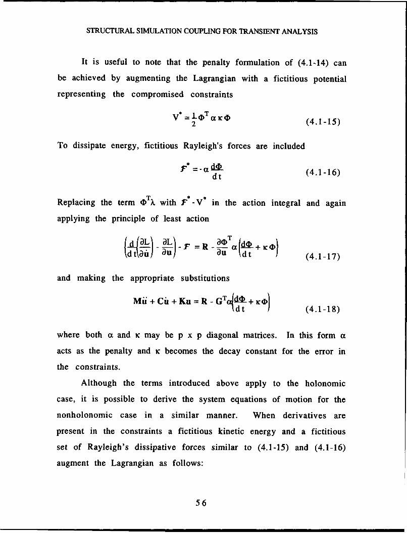
It is useful to note that the penalty formulation of (4.1-14) can

be achieved by augmenting the Lagrangian with a fictitious potential

representing the compromised constraints

V 1 (4.1-15)2

To dissipate energy, fictitious Rayleigh's forces are included

a dtDL (4.1-16)dt

Replacing the term dT)X with F - V in the action integral and again

applying the principle of least action

( -•LI- -!.F =R -- ad +

kd tkai) au d dt (4.1-17)

and making the appropriate substitutions

M6+CiC+Ku=R-GT T !t + Kci) (4.1-18)

where both a and K may be p x p diagonal matrices. In this form a

acts as the penalty and K becomes the decay constant for the error in

the constraints.

Although the terms introduced above apply to the holonomic

case, it is possible to derive the system equations of motion for the

nonholonomic case in a similar manner. When derivatives are

present in the constraints a fictitious kinetic energy and a fictitious

set of Rayleigh's dissipative forces similar to (4.1-15) and (4.1-16)

augment the Lagrangian as follows:

56

CHAFITE FOUR: CONSTRAINT EQUATIONS & NUMERICAL SIMULATION COUPLING

T 2 (4.1-19)

and

F* = (4.1-20)

Placing these terms within the action integral yields:

(ýJaL al, ~F G-0 T5

Ldtkau) aL (t =R d (4.1-21)

Making the appropriate substitutions to obtain this equation in

matrix form results in

Mii + Ci + Ku = R -HTrdttdt) (4.1-22)

4.2 The Simulation Coupling Process

The solution of dynamic problems by means of simulation

coupling requires three distinct elements. The first of these elements

is, obviously, the individual simulations for the separate fields.

Additionally, elements to evaluate and correct for any violation of

the constraints which couple the fields and to handle data

management tasks and control the execution of the separate

simulations are necessary.

There are two different ways in which the execution of the

coupling process may take place. The simplest form starts with a

57


SPrediction - Corrective Force

Evaluation "-'

[nfn+l

Field 1 Time Update Field2

Interaction Variables

Figure 4.2-1 Information Flow in Concurrent Evaluation

prediction of the field states (x and y) in order to produce a set of

corrective forces based on the incorporation of constraints. Then the

individual simulations calculate the field responses at the given time.

Finally, time is incremented and any necessary updates to the data

structure are handled. This sequence is illustrated in Figure 4.2-1. In

this case the evaluations made by the simulations may be carried out

in series or in parallel. This execution order is called concurrent

evaluation.

The second execution process is slightly more involved than the

concurrent evaluation. It also starts with a prediction of the state

variables and a corrective force prediction. However, only one field

evaluation is carried out. This execution is used to update the force

evaluation before analyzing the second field. Again, the process ends

with time update and data management functions. This is called a

staggered evaluation and is shown as Figure 4.2-2. In staggered

evaluation one field may be consistently analyzed first or the order

may be switched as seems fit.

58

CHAPTFER FOUR: CONSThMNT EQUATIONS & NUMERICAL SIMULATION COUPLING

SPrediction - Corrective Forc1

~EvaluationInfn+l 1

TimeTUpdateField 1 I- Field 2 ..

Figure 4.2-2 Information Flow in Staggered Evaluation

As introduced in Chapter Two, the dynamics of a two field

coupled system can be expressed as

Mxi + Cxi + Kxx = Rx + fcx(i,xy,y)Myy + Cyy + Kyy = Ry + fcy(X,x,y,y) (4.2-1)

where the corrective forces due to the constraints, fcx and fcy, are

found using the methods already discussed and other similar

methods. For the following discussion the forces are assumed to be

calculated using a stabilized penalty formulation. It is useful to note

that these equations are uncoupled if fcx and fcy are considered to be

unresolved externally applied forces.

Solving these equations by means of the numerical integration

was discussed in Chapter Three, the system equations become

[Mx + 5xCX + Xn =[mMxM+ cxCx + )KxKx]Xn + )Rx(Rx,n + fcx,n)( 4 .2. 2 )

[My + ByCy + 2 Ky yn= [tMyMy + ýcyCy + ýKyKy] yn + yRy(R y,n + fcy,n)

or in simpler notation

[(1-*M)MU + (W-kc)Cai + (82-k)Ku]Un = hR(Rin + fc,n) (4.2-3)

where

59


M U = M " '] C u = C T 0 , u [ 0 ] R = R xn0 M IU[ 0 Cy [ 0 Ky 1[Ry,n[

8 =[8xByfr' q.=[ ). .y ]T f.,n =[fcx,nfCyfnT ,1 = [I 1]T

Although the forms of the constraining force developed in

Section 4.1 do not require linear constraints be used, analysis of the

simulation coupling process is greatly aided by a linear

approximation as follows:

D = Cci + Kcu (4.2-4)

With such an approximation the forces of constraint are

Holonomic fc'n -KT'Kc(un + IcUn) (4.2-5)

Nonholonomic fc,n = -C1 a (Ccun + Kc tin)

The manner in which these forces are evaluated is based entirely on

the particular execution process used.

4.2.1 Concurrent Evaluation Coupling

As has already been mentioned concurrent evaluation applies

the same correction term to each field. For this term to be treated as

an applied force (allowing the simulations to remain uncoupled), it

cannot be a function of the current time step. Through use of the

predictors introduced in Chapter Three, any dependence on the

current states is removed.

First the integration approximation is applied to remove

derivative terms

60

7VNF 1 •7 . .. , - - .F.31

CHAPTER FOUR CONSTRAINT EQUATIONS & NUMEICAL SIMULATION COUPLING

Holonomic fn - -K 4aKc[I(un - hu) + X UU] (4.2-6)

Nonholonomic fc,n = -c4Cc(iUn - h ný) + Kcl4un

or in operational form

Holonomic fc'n = -KT aKc(V(.)I + ic)Un (4.2-7)

Nonholonomic fc,n = -Co (CcV(.)2 + KcV(.))Un

In this form the base states, un, are estimated using a predictor of

the form of (3.4-1). The predicted correction terms, after

substituting p(.)Un for un, are

Holonomic f, = -K~caKc(V(.)I + KC)p(.)Un (4.2-8)

Nonholonomic f, n = -Co'a(Ccy(.)2 + KcV(.))p(.)Un

Making the following definitions to simplify the notation

Ah = (W(.)I + lc)p(.) (4.2-9)

nh - (I�I(.)2 + C-'KcV(.))P(.)

Then the system equation for the concurrent evaluation is

[(1-ýM)Mu+ (8-C)Cu + (2-K)Ku +¢KcTtKcýUn = R Rn (4.2-10)

or for the nonholonomic case

[(1-M)Mu + (S-Oc)Cu + (82-)K + cLccJ Un = qR Rn (4.2-11)

The implementation of the concurrent evaluation is given as

Table 4.2-1.

61


Table 4.2-1 Implementation of Concurrent Simulation Coupling

Step in Coupling Process Associated Equation Number

1. Use states n-1 to n-m to find up (3.4-1)

2. Use states n-1 to n-m to find hnu and hun (if needed) (3.1-7)3. Use uP, hu, and hn to find f, (4.2-6)

4. Send flc,n to separate simulations

5. Separate simulations solve for un (4.2-3)

6. Calculate tin and un if simulations do not provide them (3.1-6)

7. Update time and increment n = n+1

4.2.2 Staggered Evaluation Coupling

The staggered evaluation follows directly from the concurrent

evaluation. However, since the fields must be handled in series, the

response from the first field is used instead of a prediction when

calculating the correction force for the second. The operational form

also comes from the concurrent evaluation in the following manner.

Consider first the form of the correction force, fPc,n.

fc( n(IKja~yx ((KoX)yx [(9h] 7nn (4.2-12)

or

~[(I&KL~ 0 ~~c~n (J a&ý (1 (x~ yx Ph] I Yn (4 .2 -13)

The predictor term" is expanded as follows:

62

CHAPITR FOUR: CONSTRAINT EQUATIONS & NUMERICAL SIMULATION COUPLING

I.Lh 0

I gh 0 (4.2-14)0 t•h

The upper half of this matrix deals with the prediction of each field

for evaluating the constraint forces acting on the first field; the lower

half does the same for the second field. By eliminating the term in

the lower half which corresponds to the prediction of the first field,

the actual values are used instead of predicted ones. This results in

the following matrix:

gh 00 gh

(h = (.)I + K) 0 (4.2-15)

0 g.Lh

This makes the notation for the correction force of the staggered caser 0

c,'n= " 0 (Kl' 0yX (l aKctx . Iyn ](4.2-16)

The appropriate term for nonholonomic constraints is

f,n = - [T ]h Tn

L ~~QCC 0 aacQ1(acYX I (4.2-15)

where

9nh 0

o •tnh9nh -- 20 - (4.2-16)(I4K.) + Cc Kc,4.)) 0

0 Itnh

63


The implementation of the staggered evaluation is given in

Table 4.2-2.

Table 4.2-2 Implementation of Staggered Simulation Coupling

Step in Coupling Process Associated Equation Number

1. Use states n-1 to n-m to find uP (3.4-1)

2. Use states n-1 to n-m to find hnu and hl (if needed) (3.1-7)3. Use un, hu and h} to find f, for x field (4.2-6)

4. Send ftc,n to x field simulation

5. Simulation solves for Xn (4.2-3)

6. Use yP, hY, hn•, and Xn to find fP, n for y field (4.2-6)

7. Send fPn to y field simulation

8. Simulation solves for yn (4.2-3)

9. Calculate 6n and iin if simulations do not provide them (3.1-6)

10. Update time and increment n = n+1

4.3 Analysis of the Simulation Coupling Process

4.3.1 Stability Analysis of Simulation Coupling

Having developed operational expressions for the system

equation of motion, the stability analysis is fairly straight-forward.

There are two possible methods to accomplish the analysis. Both

consider the unforced response (Rn = 0 for (4.2-11)) and develop a

system characteristic matrix. Since the response is unforced the

eigenvalues of the matrix must be less than or equal to unity, to keep

the response from growing with time. Although both methods will

64


be shown in detail in the examples of Chapter Five, they will be

briefly introduced here.

The first method uses the matrix, C(z), which is the matrix

multiplying un in (4.2-11). For instance, the characteristic matrix for

the concurrent evaluation and nonholonomic constraints is

C(z) = (1-ýM)Mu + (&-Wc)Cu + (8 2 -k)Ku +' ýR KTcKKc.nh (4.3-1)

Taking the determinant of this matrix produces the characteristic

polynomial, C(z). The simulation coupling process is stable if the

roots of C(z) lie within the unit circle. Optimally, it is desired that

these roots reflect the same stability as the fully coupled system. An

example of this would the trapezoidal rule; an optimally stable

coupling process would keep this method's A-stable characteristics.

The second method relies on a time domain analysis and is a

common numerical analysis procedure (see [4.7]). The state variable

un can be written as a function past state variables and derivatives

using a form of (3.1-9)

[M+ 8C + 2K]un =[M + 8(C- A1'B)]h u + 5A'Xhv + 2fc (4.3-2)

Using the integration approximation for u and (4.3-2) to substitute

for un, the derivative tin can also be written as function of past

states. The definition of the auxiliary vector and integration

approximation for v provide vn and v in terms of the past states.

These equations make it possible to write a matrix which when

multiplied by the vector [ Un-1 Vn-1 Un-2 Vn-2 ... Un-m Vn-m ] will give

the vector [ Un Vn Un-1 Vn-1 ... Un-rm+1 Vn-m+l ]. The roots of this

65


vector must also be less or equal to one for the coupled simulation to

be stable. Although developing this matrix is more difficult than

finding C(z), then eigenvalues may be calculated directly from this

point without first taking the determinant to find the characteristic

polynomial.

Unfortunately using these methods is not nearly as easy as it

would seem. Large coupled problems tend to have thousands of

degrees of freedom, and the number of roots to the characteristic

equation can be several times that number. This makes calculation

of these roots difficult even with computer methods. Additionally,

the only parameters the dynamicist has available to ensure stability

are the integration time step, the choice of the predictor, and the

penalty used to find the corrective force. The choice of overall

penalty is generally governed by requirements to keep the

constraints violations very small and the time step must be small

enough to stabilize the high frequency poles associated with the

application of a penalty. This leaves only the predictor and at this

time there are no guaranteed choices for optimally stable predictors.

4.3.2 Accuracy Analysis of Simulation Coupling

The accuracy analysis also involves manipulating the

characteristic equation, but this time the s domain form is desired.

By expanding the exponential terms in the operational expressions,

e-sh = 1 - sh + 0.5(sh) 2 - ... , the characteristic equation may be

written in powers of s. This allows the characteristic equation in s to

be transferred back to a differential expression and from there to a

standard eigenvalue problem. As an example consider an undamped

66


system integrated using the trapezoidal rule and computational path

2. The characteristic equation is

[(,M + 82K]un = 0 (4.3-3)

Substituting for the operational expressions from Chapter Three

(l _e-shJ M + K~u"=OS+ eshl (4.3-4)

Expanding e-sh

[(I - 4(sh)2 + O(sh)ý s 2+Kiun = 0

This will give the differential equation

Mi -h 2 Mu'+ O(u(4))+Ku= 06 (4.3-6)

or an eigenvalue problem

(M +-Ih2K + .. h)2 _ O(wh)4 + K = 06 (4.3-7)

These equations show that, as expected, the trapezoidal rule

introduces no artificial damping but does produce a certain amount

of frequency distortion. The same sort of analysis may be carried

out on the simulation coupling characteristic equation. The

numerical values can then be compared to similar values obtained

for the fully coupled system.

67


68

Chapter Five

Illustrative Numerical Examples

Although the si. :lation coupling theory is aimed at the

solution of large scale problems, it is not possible to show all the

details of analysis of such problems. For this reason the following

chapter is organized to present a series of smaller dimensioned

problems in which the all of the aspects of the theory presented are

shown. The first example is the one dimensional motion of a single

rigid body. The response is considered subject to different forcing

conditions. The second example is a more complicated model

representing a satellite held at the end of the shuttle's manipulator

arm. This example shows some of the effects of imposing constraints

on a flexible domain. Finally, the single rigid body is again

considered. All six degrees of freedom are allowed to show the

interaction between translational and rotational motion in the

presence of constraints. All examples use the concurrent evaluation

along with a stabilized penalty format to find the constraint forces.

69


5.1 One Dimensional, Single Body Example

As a single body example consider the structure illustrated in

Figure 5.1-1. This body is representative of a dual spin stabilized

satellite (see [5.1]). The mass properties for each section are

Rotor = 700 kg Platform = 300 kg

Each center of mass (CM) is located on the spin axis. The platform

CM is 0.5 m up from the joint between the bodies and the rotor CM is

0.75 m down from the joint. The complete center of mass is 0.375 m

down from the joint.

The inertia properties of the satellite about their CMs are:

Spin TransverseRotor 350.0 kg-m 2 306.25 kg-m2

Platform 150.0 kg-m 2 100.0 kg-m 2

Complete 500.0 kg-m 2 734.375 kg-m 2

Tp ,,Platform

lm I P

i RotorTransverse _

1.5 mn ± r

- 72m

70

CHAPTER FIVE: ILLUSTRATIVE NUMERICAL EXAMPLES

Figure 5.1-1 Satellite Rigid Body Model

The satellite is subject to the following forcing conditions

resulting from attitude control type maneuvers:

Forces = 1 N any axis Torques = 10 N-m about spin

The forces and torques are applied on the rotor section. For the

purpose of simulation coupling the single body is divided into two

separate rigid bodies where the platform joins the rotor.

5.1.1 Analysis of 1-D Example

Considering the response of each body in the direction of the

spin axis, the equations of motion are

Mrxr = Rr and Mpxp = Rp (5.1-1)

Additionally, the bodies are rigidly connected along the spin axis, or

Xr - xp = 0. By applying the stabilized penalty method discussed in

Chapter Four, the following constraint forces are found:

Tfc = -[1 -1]T [(Qr-ip) + c(Xr-Xp)] (5.1-2)

Adding these forces to the system leaves

[Mr O](Xr}(Rr0 +f( -0 Mp ip Rp (5.1-3)

Subtracting the second equation from the first and rearranging

terms produces the constraint error equation(kr-ip) - a M' (xr---- + •CK M' (X,-Xp) = Rr - R--

rp MrMp X Mr Mp (5.1-4)

The penalty K controls the steady state error

W M 0 t I(xr-Xp)s 4 -JRrMp - RpMr

MrMp MrMp (5.1-5)

71


With the given mass properties and a requirement that the steady

state error be less than 1.OxlO-7 meters

c= l .3.0x l105a0 (5.1-6)

The other penalty, a, determines the damping ratio of the error. For

a ratio of 0.3, a = 2400.0 which leaves ic = 125.0.

The equations of motion may be integrated following the (0)

computational path and using the trapezoidal rule

Wn - Wn. 1 = 0.5h(wn + xirn-1) (5.1-7)

Using this equation to substitute for the accelerations in (5.1-3) gives

Xr r + h ( . r + 2(+ Mr 0 R; + (fc)n (5.1-8)Ipn =Xp In-X /X1 4[ _I 'Pn. 0 MP Rp n

The constraint force is found using a last value predictor, xPn = Xn.1,

leaving

fc,n - 1'[r + K(xrn"] (5.1-9)-1P n 1 -LXpn-P

These two equations are used to carry out the simulation.

To perform the analysis of the simulation coupling the notation

introduced in Chapter Three is used. Defining u = [Xr Xp ]T, Rr = 0,

Rp=0, and M= Mr 0 leaves0 MpJ

Un = Un-I + h6in-+- -2 h2M"1 - [[ 1n-1 + KUn-1] (5.1-10)4 4

72

OCIHAPR FIVE: IJuSTRATIVE NUMERICAL EXAMMlES

Using the characteristic equation for holonomically constrained

coupled problems listed in (4.2-10)

[(1-NM)M + aORK TKc(AV + IC)p(z)] Un = 0 (5.1-11)

For this example the last value predictor is characterized by the shift

operator, z- 1, and the polynomials 4m and ýR are listed in Table 3.3-1.

Making the appropriate substitutions results in the following form:

[(SV)M + a(8V1)KTKc(V + K)zIO] Un = 0 (5.1-12)

The operational notation for the trapezoidal rule is found in Section

3.5. Using the given polynomials and clearing most fractions leaves

Z(Z-I)2M ak!KJ(z-)(z+1) + ý+)2]]uO[z(z-1)2M+ 2K-1z + h-(z+i1 (5.1-13)

From the form of the constraint, (D = Xr - xp, the matrix K c is found to

be [1 -1]T. Expanding the polynomials and matrices gives the

characteristic matrix equation, C(z)

C(z) = [(z3_2z2+z)[ Mr 0 ]+ hl[-1][(l+)hZ2 +(ich)z+(X-- -1)1 (5.1-14)0 MpI 2 -11lJ 2) 2

Defining a temporary variable, a(z)= (l+--z2 + (ich)z +(1-- -)

~i-a)2) 1Mr(z 3-2Z2 +Z) + 2h a(z) - QhLa(z)C(z) =2 2 (.-5

- 2h'a(z) Mp(z 3-2Z2 +Z) + --h a(z) (5.1-15)2 21

For stability, the roots of the determinant, det(C), must be within the

unit circle. Taking the determinant

73


2F-) ((,M 21 ~ d2~ 1 d 2~

z~z~1j11- +(o a1iLpch M J 2 ~ 1h) +1zjMToJa-t 21ý44

(5.1-16)

Since the first three roots (z = 0,1,1) do not vary with a, r, or h,

they are not as important as the remaining three. For the penalties

given, Figure 5.1-2 shows two of the remaining three roots moving

away from z=1 as the step size is varied from 0 to 0.008, where

0.008 is at the point of instability. The third pole moves from the

origin toward a value of z = 0.02. The desired time step should be as

large as possible while still being stable. For this reason h is chosen

to be 0.005.0.3 .

' -'- h 0.008

0.2 h=O.005 -

0.1 * h =O 0.002

h =0.0010h=--O h=O

-0.1 ..

-0.2 -

-0.3-0.7 0.8 0.9 1 1.1 1.2 1.3

Figure 5.1-2 Pole Locations of Rigid Body Model

The choice of a does not seem to have a great effect on the

overall stability. If a is doubled the limiting time step increases by

less than 5%. Therefore, since a is proportional to the damping ratio

and large damping ratios mean small overshoot, it is often feasible to

increase a by as much as a factor of five. Additionally, changing the

74

CHAFFER FIVE: ILLUSTRATIVE NUMERICAL EXAMFS

mass ratio of platform to rotor does not have any effect on the

coupled simulation stability. On the other hand K has a great effect

on stability. Doubling the value of Kc will almost double the stable

time step.

5.1.2 Response of 1-D Example

The response is considered subject to three separate forcing

conditions; a constant force input, a ramp input, and a pulse sequence

input. In each case the responses of the rotor and platform are

compared to the response of the complete rigid case for a two second

run. The time step used is h = 0.005 and the penalties are those

suggested in the previous section. The position, velocity, and

acceleration for the constant forcing case are illustrated in Figure

5.1-3.

The error between the coupled and complete response is

noticeable only in the acceleration plot and then only during the first

two seconds. The steady state error settles out to exactly 1.0 x 10-7

as desired. To check the calculated stability boundary, a coupled

simulation was made with h = 0.008. The constraint error and the

constraint error rate are shown in Figure 5.1-4.

The second forcing condition is a ramp thrust from 0 to 1 N

over a two second period. The position, velocity, and acceleration for

this case are presented in Figure 5.1-5. In this case the constraint

error also increases with time reaching a final value of 1.0 x 10-7.

75


0.002-........... Complete........... Rotor

- Platform

. 0.001

0.000-i0.0 1.0 2.0

Time

0.002-.......... CompleteS.......... Rotor

Platform

S0.001'

0.0000.0 1.0 2.0

Time

0.002-.......... Complete........... Rotor

Platform

S0 .0 0 1 ...

0.000•0.0 1.0 2.0

Time

Figure 5.1-3 1 -D Example Response to Constant Forcing

76

4 7~~7"W7 7

CHAPER FIVE: ILLUSTRATIVE NUMERICAL EXAMPLES

6.0e-6

•: 4.0e-6, -

"= 2.0e-6

. 0.Oe+0-

-2.0e-6

-4.0e-6

0.0 1.0 2.0Time

2.0e-4 -

1.0e-4,

0

>0.0e-0

t-:

W -1.0e-4

-2.0e-4 •0.0 1.0 2.0

Time

Figure 5.1-4 1-D Example Constraint Error, h - 0.008

The third forcing condition is a series of 1 N thrust pulses. Each

pulse lasts a quarter second and separated from the next pulse by

the same interval. The position, velocity, and acceleration for this

case are illustrated in Figure 5.1-6. Some noticeable differences

occur in this case due to the rapidly changing input. However, the

coupled position and velocity still track the actual solution fairly

well.

77

STRUCT7URAL SIMULATION COUPLING FOR TRANSIENT ANALYSIS

0.0008.........Complete......... Rotor

0.0006- Platform

0.04

0.0002-

0.0000*0.0 1.0 2.0

Time

0.0010. .........Complete

0.0008 . ........ R to

Platform

S0.0006-

:> 0.0004-

0.0002-

0.00000.0 1.0 2.0

Time

0.0010-......... Complete

0.0008 . ........ R to

Platform

*~0.0006-

o0.0004-

0.02

0.0002

0.0 1.0 2.0Time

Figure 5.1-5 1 -D Example Response to Ramped Forcing

78

CHAFFER FIVE: ILLUSTRATIVE NUMERICAL EXAMPLES

0.0012- S........... C m ltComplete

0.0010 ....... Rotor.- Platform

0.0008

.u 0.000600.0004

0.0002-

0.0000•0.0 1.0 2.0

Time

0.0012............ Complete

0.0010- RotorPlatform

0.0008

"• 0.0006

0.0004

0.0002

0.0000,0.0 1.0 2.0

Time

0.004 ........... Complete

S........... Rotor

Platform

= 0.002

S0.000 -' ...

-0.002•,0.0 1.0 2.0

Time

Figure 5.1-6 1-D Example Response to Pulsed Forcing

79


5.2 One Dimensional Shuttle-Satellite Example

The next example is the one dimensional, four mass model of a

satellite held in the space shuttle manipulator arm illustrated in

Figure 5.2-1. In actuality the connection between the end effector of

the arm and the satellite platform is assumed rigid, and this will

provide the coupling between the separate fields of the shuttle

dynamics and the satellite dynamics. The shuttle partition is made

up of the shuttle and the manipulator arm. The one dimensional

idealization of the flexibility in the arm is a spring connecting the

two masses. The satellite partition is similar to the satellite in the

previous rigid example with the addition of a small amount of

flexibility between the rotor and the platform. The masses involved

are

Shuttle Body (Ms) 85,000 kgManipulator Arm (Ma) 140 kgSatellite Platform (MP) 300 kgSatellite Rotor (Mr) 700 kg

The flexibilities involved areManipulator Flexibility (Ka) 300 N/m

Satellite Flexibility (Krp) 1800 N/m

Shuttle Partition Satellite Partition

K R

I I

I I

% ,

! ~It

Rigid Connection

80


Figure 5.2-1 1-D Shuttle-Satellite Model

Forces are allowed to the system from the control jets on the shuttle

and the satellite. The satellite jets are capable of the same 1 N thrust

while the shuttles jets can deliver up to 2 kN (see [5.21 and [5.3]).

5.2.1 Stability Analysis of Shuttle-Satellite Example

The equation of motion for each partition is

[s 0 ~ -K(:}a K](xs) =(Rs}

and M ij) +[ Krp oI(5.2-1)and 0 Mr Ir -Krp Krp Xr Rr

The complete system equation of motion found by eliminating a

degree of freedom due to the rigid connection, Xa -xp = 0

oS 010 I sF Ka~ -Ka 0 1xsl (Rs~

0 Ma+Mp 0 Xp + -Ka Ka+Krp -Krp XP = (5.2-2)0 0 Mr Xr 0 -Krp Krp Xr Rrl

The equivalent simulation coupled system with corrective constraint

forces is

[M3 0 0 0 Ka-Ka 0 0 Rs

Ma 0 0 i -Ka Ka 0 0 xa fc

0 0 MP 0 Xp 0 0 Krp -Kp Xp 4fX rL0 0 0 Mr x l 0 0 -Krp Krp JRr

(5.2-3)where the constraint force is

fc = - a [(Xa-Xp) + Kc(Xa-Xp)] (5.2-4)

81


To determine the penalty constants, a and Kc, an error analysis

similar to the one used in the first example is done. Subtracting the

third line of (5.2-3) from the second

(ka -p)+ K' (Xa - Xs) - Krp(Xr- Xp) = Ma+ Mp fc

Ma MP MaMp (5.2-5)

Rearranging terms, defining e = Xa - Xp, and substituting for fc

M + Ma +MKrpx____ KKe+ac Me + ai Me= -- R r -Xp) -- "(Xa -Xs)

MaMp MaMp MP Ma (5.2-6)

Replacing the terms on the right hand side with terms from the first

and fourth lines of (5.2-3) leaves

Ma+MP Ma+MP (Rr- Mrxr) (Rs- Msxs)e+a e ac e =

MaMp MaMp MP Ma (5.2-7)

Using (5.2-7) to require the steady state error be less than 10-6

meters,K=1.1.5.108

a (5.2-8)

The other penalty, a, determines the damping ratio of the error. For

a ratio of 0.1, a = 24,000.0 which leaves K = 6,250.0.

Since using C (z) to do the stability analysis would require

taking the determinant of a 4x4 -natrix of third order polynomials,

the second method of determining stability is used instead. Applying

the trapezoidal rule and a last value predictor, (3.1-9) becomes

[M + 82Klun = B2Wn-1 + 28MU.n- 1 + Mun-1 + 82fc,n (5.2-9)

82

CHAPTER FIVE: ILLUSTRATIVE NUMERICAL EXANM

where M and K are the defined in the coupled equation (5.2-3).

After substituting for fc,n

[M + 2K]Un = 82Min_l + [28M - o8'2G]tin4l + [M- a52G K]Un-1 (5.2-10)

where G = = [ 0 1 -1 O]T[ 0 1 -1 0]. Using the the trapezoidal

rule i'. may be written

un = " 1(un - un-x) - uin-I (5.2-11)

or using (5.2-10) for un

[M+8 2K] Un = 8Mii.n-I + [M 82K o-a8G]jUn-1 +[-8K-c8Gic]un..1 (5.2-12)

Doing the same thing for uin

EM + 62K]iin = [_52K]iinl + [-28K - (G]6in.l + [-K- aGclunI (5.2-13)

Defining KEff= EM +82K] and using (5.2-10,-12,-13) leaves the

following amplification matrix relating states at tn-1 to states at tn:

[ KE•-8f2KK] Kll[-28K- ozG] I -K- aGic][ K'Eff8M K'EfIM - 82K- ax8G] KI• -8K- a5Gic] (5.2-14)

KICEý8M l•K[28M - a8 2G] KI• _a8M - Gi

All of the eigenvalues of this matrix must be within the unit circle to

ensure the coupling process is stable. Performing this analysis, the

maximum time step that maintains stability is h = 1.50x10- 4.

5.2.2 Accuracy Analysis of Shuttle-Satellite Example

The characteristic equation for an undamped structural system

with holonomic constraints is

83


[(1-M)M + (5 K + a)RG(V + K:)p(sh)]Un 0 (5.2-15)

For the 0 computational path using the trapezoidal rule and a last

value predictor the following constants are defined:

OM-l-'=', 2K =-8'V R=' 8-1, p(sh)=e , V=tandsW

With these constants (5.2-15) becomes

[8tanh(s h)M + 8 tanh-W (shK + ot~tanh '(1JL)G(tanIjs hl + K)eS ]n = 0(2 )•27 2=0(5.2-16)

or after clearing fractions

[tanh2(ý_h)M + K+ a G(tanh(5-k) + 1c)esh] Un = 0 (5.2-17)

Using the series expansion for tanh and e

tanh s h)= s(1 _-1s2h2+-Ls4h4 .. ) and esh= (1+sh+l-s2h2+Ls3h3+±ls4h4+...112 240 2 6 24

which makes the complex terms

tn2(S h)= S$ 1-Ls2h2+ 11 s4h4_....tan( 2 6 720 - h

tanhts )eSh = s++sh+5s2 h 2+ l__.s 3 h3+ 1..s 4 h 4+.-..

S12 12 240

Inserting these terms into (5.2-17) leaves

MS212--LS2h2+ 11 s4h4_..)+ K6 720

+ aGs 1 + sh _-__ s2 h 2 + .J s3h+ __1 s4 h4 + ... = 0=

12 12 240

+ aG l+sh+is2h2+Is3h3+ ls4h4+-.. (5.2-18)L 2 6 24

or rearranging terms

84


2 2 3 2 4 2 -

(M-hi-Ms +aGh+aGii-s +O(h )s26 12

2h 2+Kh' )2 4+ (G(l+ih)+aG 12 h +6 ) +O(h )hs Un = 0

( 2 2 4) (5.2-19)+ ~K+aGK+lL-a~csGC + 0(h)

Dropping higher order terms and using the fact that [Ms2 + K]un = 0

2 32(M -hi-K+aGh+ocG'iM KJ h

6 122 2 3

+ (G(l+rh) +aG(5 h h + iL)M K s Un = 0612 6h2 -1' (5.2-20)

+ ýK+aGIK+ h aGflcMK)]2

This equation can be used to find the coupled system frequencies.

Table 5.2-1 compares the continuous system frequencies to the

frequencies shifted by integration alone (discrete frequencies) and

the frequencies shifted by integration and coupling. As (5.2-20)

shows some artificial damping occurs as a result of the simulation

coupling process. However, the damping ratios of the coupled

frequencies is less than 10-7. The is also a coupled frequency

corresponding to the constraint penalties at approximately 1200

rad/sec.

Table 5.2-1 Comparison of Frequency Shifting Effects (rad/sec)

Continuous Discrete Coupled

0.00000000 0.00000000 0.00000000

0.50034156 0.50034155 0.50034119

2.66408400 2.66408398 2.66408308

85


5.2.3 Response of Shuttle-Satellite Example

Two different responses were considered for this example.

Both cases involved forcing the system using the shuttles control jet

thrusters. Each run is compared to the identical conditions using the

complete system shown in (5.2-2). For both, the complete and the

coupled systems, a time step of 0.0001 seconds was used. The

penalties suggested in Section 5.2.1 were used for the coupled case.

The first case is a 20 second run where the force of 2 kN has

been applied for the first second. Figure 5.2-2 shows the position of

the shuttle, the satellite rotor, and the joint between the arm and the

platform. Additionally, Figure 5.2-3 shows the constraint error and

constraint error rate for this case.

Since this is an undamped example the system energy should

be constant. However, due to the stabilization of the constraints,

energy will be bled off from the system. This process will continues

as long as there is any potential energy stored due to flexibility. This

artificial damping is a very slow process and has little noticeable

effect, but care should still be taken to make the damping ratio for

constraints less than or equal to the damping present in the

structure, if possible.

The second case should show that no significant energy is lost

even over a period of many time constants. It is a two minute run

where the 2 kN force is applied for ten seconds. The figures for this

run shows a twenty second period at the end of the two minutes.

Figure 5.2-4 shows the translations of the major system parts.

Figure 5.2-5 illustrates the error between the coupled response and

the complete response for the shuttle, the rotor and the end effector.

86


0.5. ........... Complete

0.4 - ------ Coupled

S 0.3-

o 0.2--

0.1-

0.0-0.0 10.0 20.0

Time

0.5-S........... Complete - End Effector

S0.4- Coupled - ArmCoupled - Platform

S0.3

0.20"U,,

o 0.1

0.0-0.0 10.0 20.0

Time

0.5_

S........... Position - Rotor

0.4 - .-...... . Coupled

0.3a• 0.3 -

• 0.2

0.1

0.00.0 10.0 20.0

Time

Figure 5.2-2 Shuttle-Satellite Example Short Term Response

87


le-7

0e+0-

-le-7

0.0 10.0 20.0Time

6e-8

4e-8

• 2e-8

> 0e+0

S-2e-8

-4e-8

-6e-8'0.0 10.0 20.0

Time

Figure 5.2-3 Shuttle-Satellite Example Constraint Error

88


24.0---. 0 ........... Complete

23.0 . ........... Coupled

22.0

• 21.00

20.0 ..

19.0'100.0 110.0 120.0

Time

24.0-S........... Complete........... Coupled - Arm

S23.0-SCoupled - Platform

W 22.0

21.0

20.0

19.0 -

100.0 110.0 120.0Time

24.0. ........... Complete

23.0 ---------- Coupled

S22.0-

S21.0 -

20.0

19.0'100.0 110.0 120.0

Time

Figure 5.2-4 Shuttle-Satellite Example Long Term Response

89


3e-6

2e-6

Sle-6

0e+0

• -le-6'

-2e-6

-3e-6

100.0 110.0 120.0Time

3e-4Arm

2e-4 - -------- - Platform

o le-4

• Oe+0w

-le-4

W -2e-4

-3e-4100.0 110.0 120.0

Time

3e-4

2e-4

Sle-4

0e+0

m -le-4

-2e-4

-3e-4100.0 110.0 120.0

Time

Figure 5.2-5 Shuttle-Satellite Example Long Term Error

90

5.3 Free Floating Rigid Body Example

The final simple example is a return to the satellite described

in Section 5.1 and illustrated in Figure 5.1-1. This example, however,

will consider all six DOFs, Ro = [ X Y Z IT and 0 = [ 01 02 03 IT. The

translations express displacement from the inertial frame in inertial

coordinates and the angles represent Euler angles of a 2-1-3 rotation

from the body frame to the inertial frame. The equations of motion

for a rigid system with these specified DOFs are derived in many

dynamics texts (see [5.4]).

For the fully rigid case there are six active constraints. Three

translational constraints require the point where the rotor joins the

platform to have the same inertial position. Three rotational

constraints require the Euler angles for the platform orientation and

the rotor orientation to be equal. The two sets of constraints are

distinct enough to justify having a unique a and K for the translations

and the rotations.

5.3.1 Analysis of Rigid Body Example: Translational DOFs

Each body frame is fixed at the body CM with the z axis

oriented along the spin axis indicated in Figure 5.1-1. If ra is the

position of the joint between the platform and the rotor with respect

to the CM of frame a in frame a coordinates. With this definition the

constraints on the translational DOFs are

S=Rr- RoP+ICBrr -ICPrP (5.3-1)

91


where ICB is the matrix representing an orthogonal 2-1-3 rotation

from body to inertial frames. Taking the first two derivatives givesd= =Rr- S~o + I(Wrr+ ICrp c(rxrr) - IC(opxrp) (5.3-2)

dt

and

2 = o -r + IIrBrr I3rp + Ilr(frxrr) - IC(OPxrP)

dt r (5.3-3)+ ICB (rxrr) - ICP (PxrP)+ IC (orx (rxrr)) - iCp(0Px (PxrP))

These terms are used to form the constraint correction force, fc, and

the constraint error equation.

The translational equations of motion for these two bodies are

- and R-_ -" 1mr Mr +c (5.3-4)

Taking the difference of these equations and substituting e for D and

-c (d,-t + Ic for fc leaves

"Ro- Ro= IICRr mr+mp[e+Kie]

mr mrmp (5.3-5)

Adding the additional terms to form e and the constraint error

equation

j+mr+mP a o + mr +mP a _ice -rICrar +mrmp mrmp MT (5.3-6)

where f* includes the nonlinear terms treated as applied forces

f* =I�jB rr Ir rP + IfrB( rxrr) - Ie(wPxrP) + IcB(orxrr)

-ICP (dPxrP) + CB(0rx(worxrr)) - ICP(wPx(wPxrP)) (5.37)

92


In order to keep the analysis linear, the nonlinear forcing term

is assumed to be much smaller than the actual forcing. This leaves

the vector form of the error equation found in (5.1-4). Given the

same error limits and desired damping (steady state error less than

10-7 and damping of 30%), the penalty constants and time step limit

found in the first example will still hold. These numbers are

a = 2,400.0 K = 125.0 h __ 0.008 (5.3-8)

5.3.2 Analysis of Rigid Body Example: Rotational DOFs

As described earlier the rotational constraints require the Euler

2-1-3 angles for each frame to be equal

D = Or_ op (5.3-9)

Taking the first two derivatives gives

d 0 =r _ 0P= Srlcor - Splc0Pdt r - (5.3-10)

and

0 0p=Srlcr- Spl6p +Sr I r- Splo p (5.3-11)dt

2

where Sr is a non-orthogonal transformation from Euler angle rates

to angular velocity coordinates (see [5.4]). These terms are used to

form the constraint correction torques, rc, and the constraint error

equation.

The rotational equations of motion for these two bodies are

93


I rlr',r Irl(corxIrrr)+ Ir-'c

COp (P p ) - l=-l rc (5.3-12)

Premultiplying by the appropriate form of Sa1 and taking the

difference of these equations, as well as substituting e = (D and

"c= -Saa[•-+ i,] leaves

Sr16r _ S Sp 1(0 p = Sr 1(Sr + Sp)SpI'r (Ir + Ip)Ip (CoPxIpoP- r.0-rxlrcor)

-Sr I(Sr + Sp)Spl'Irl(Ir + Ip)Ipl(Sr+ Sp)a[ie + ice] + Srllr lr(5. 3 -1 3 )

Adding the additional terms to form i for the constraint error

equation and making the following definitions: S = Srl(Sr + Sp)SpI and

I = If 1(Ir + Ip)lp1, leaves

e + SI(Sr+ Sp)ae + SI(Sr+ Sp)a ice = Srl'rllr r+ r"* (5.3-14)

where t* includes the nonlinear terms

"t* =SI(CoPlpP-cop orxIro~r)+ Sr !O0r- Sp1COP (5.3-15)

Two assumptions are made to keep the analysis linear. First, the

nonlinear forcing term, t%, is assumed to be small with respect to the

actual forcing. Additionally, since the error between the Euler angles

is forced to be small, the transformation matrix for the two body

frames is assumed to be the same, Srp. This will reduce the matrix S

to 2Srp,. Rearranging the remaining linear terms leaves

S i-1 S - .Sr Srpe + 4oae + 4caice= S.'rIp(Ir + Ip)'lcr (5.3-16)

94


Using this equation and desired values for steady state error and

damping ratio, the penalty constants can be found in the same

manner as the first and second examples. With a steady state error

of 10-4 degrees and and damping ratio of 0.1 the constants are o =

375.0 and K = 40.0.

To find the maximum stable time step the complete equations

of motion must be formed. Combining (5.3-12) and the fact the Sa

relates Euler angle rates to angular velocity, the complete first order

unforced equation of motion can be formed

6r0 0 0 0 Wr Ir '(0rX 1,0r)

4r o oT o6P0 0 0 0 Il ) I; 1( ()PXIPO)P)

or redefining terms

0 = K0 - *-GcI[+ K] (5.3-18)

Using the trapezoidal rule and a last value predictor, an amplification

matrix similar to the one in (5.2-14) can be formed. With K Eff

defined as 1(12)- 8K, the matrix is

[ K18K - aG] K-E'[K - aG i]1

EfI2- aG] KEfI - aGic] ] (5.3-18)

95


By requiring the eigenvalues of this amplification matrix to be within

the unit circle the critical time step is found to be h = 0.03.

5.3.3 Response of Rigid Body Example

For the response me penalties used are

a K

Translation 2400.0 125.0

Rotation 375.0 40.0

The maximum time step is 0.008 seconds and the actual time step

used is 0.005 seconds. The satellite (rotor and platform) is given an

initial spin rate of 0.5 rpm. The complete set of plots, all degrees of

freedom and errors, is given in Appendix A.

The first case reflects a constant force input of 1 N in the z axis

Due to the satellite's symmetry this forcing only excites the z axis

translation. The error response is exactly as shown in the first

example, with constraint error damping oat at two seconds to the

steady state value of 10-7 meters. The second case is similar with a

constant torque input of 10 N-in about the z axis. Again only the 03

DOF shows any response. This response damps out after four seconds

to a steady state value of 10-4 degrees. These responses show that

the simulation will perform as desired under the simplest of forcing

conditions.

Although the earlier cases verify performance of the coupling

algorithm the more interesting cases arc those designed to show the

cross-coupling effects between the translation and rotation DOFs.

The third case, a I N force along each axis shows one new effect. The

constant spin about the third axis produces a long period

displacement error in the x and y axes. This displacement is a

96


maximum at 1.5xl06 meters, larger than the desired value but still

small enough that the penalty constants do not need to be changed.

Had this value not been sufficient the constants may be changed

easily. For instance, if the maximum allowable error is 10-6 meters

then by raising K by a factor of 1.5 and a by T7.5 then maximum is

reduced while still still maintaining reasonable damping.

Additionally, if the penalties are changed by a significant amount it

may also be necessary to adjust the time step.

The final case involves applying a 0.1 second 1 N-m torque to

one of the non-spinning axes. In this case the nonlinear terms which

were ignored in the analysis of Section 5.3.2 start to have a

significant impact on the motion. The original constants must be

altered to account for this nutation of the spinning satellite and

ensure the stability of the simulation coupling process. Running

several different penalty combinations, simply adding a large

amount of damping seems the most effective correction for nutation

effects. After achieving stability, the penalties are modified to keep

the steady state errors small. The total of these two corrections

raises a by a factor of forty and K by a factor of four. The time step

is dropped during this process to 0.0025, again to ensure stability.

There is one final effect of a rigid body simulation to discuss.

When using Euler angles it is possible to encounter singularities

where the three angles condense to one DOF. This continues to be the

case in a simulation coupling process. The most successful way to

correct for this effect is to switch to a different Euler angle

combination when close to a singularity. Although this will

97


successfully avoid the singularity problems, for this example the

initial conditions were altered instead to avoid any singularities.

5.4 Conclusions from Simple Examples

These examples should show that for small cases it is possible

to write an error equation to find appropriate penalties and to

complete a linear stability analysis to find a time step for the

simulation coupling algorithm. Both rigid and flexible problems

display unique difficulties to watch for as larger, more involved

problems are attempted.

For rigid cases the most difficult problem to handle is the

singularities Each simulation handles them differently and it may

be necessary to change constraints and even penalties to account for

the singularity. The only other noteworthy problem is how to deal

with the coupling between displacement and rotation DOFs which

may occur due to rotating frames, nutation, or simple geometry

considerations. However, by making small adjustments in the

penalty constants and time step these difficulties can usually be

handled.

Simulation coupling of flexible cases presents the unique

problem of an additional dissipative force in the penalty stabilization

scheme. Care should be taken not to significantly alter the system

damping ratio, otherwise the constraint error will damp out but the

response will not converge to the correct solution.

Finally, both flexibility and rotation effects produce significant

long period error responses. This long period motion is usually much

98


larger than predicted steady state maximum values and a check

should always be made for this sort of constraint error mode.

99


100

Chapter Six

Space Station Example

The Space Station Assembly Complete model used in this

example consists of 3852 degrees of freedom and 1577 elements. It

is made up of three primary bodies: the center span and two

articulating "wings". The individual bodies are separated at the

alpha joints pictured in Figure 6.1 and the gamma and beta joints are

modelled as fixed. Since it is possible to set up the complete three-

body multibody problem for comparison the Space Station makes a

good test case for the validity of simulation coupling as an

alternative simulation strategy.

For the purpose of simulation coupling the response of each

body is calculated according to the single flexible body equations

presented in [6.1]. One individual rigid-flex one-body simulation is

used for each of the separate bodies. The simulation makes use of a

popular fourth order Runge-Kutta integration scheme instead of the

linear multi-step methods which are suggested in Chapter Three.

Additionally, the Space Station is too large for a flexible analysis like

101


Port PVAirays Starboard PV Arrays

8159 8134 8115 8150

Port Alpha Joint Starboard AlphaNode 364 JitNd 0

CMG Node 418

8165 8146 8127 8156

Figure 6.1. Space Station Freedom Assembly Complete

the one used in Section 5.2 to be done. Because of these two factors

the approach taken is slightly different than the examples of the

previous chapter.

For the non-articulated simulations all 6 DOFs at each alpha

joint are rigidly constrained. The articulated simulations allows free

rotation about the y axis (02 degree of freedom). The penalties, a

and K are to be designed to keep the translation constraint violation

less then 10-8 feet and the rotation constraint violation less than 10-6

degrees.

6.1 Analysis for the Space Station Example

As has been mentioned the flexible model of the Space Station

is too large for a full analysis. It is still reasonable, however, to do

the rigid body analysis. This will allow a first guess at the complete

model penalties using the rigid body penalties. If this guess should

prove unacceptable then further adjustments can be made based on

the error responses.

102

CHAPTER SIX: SPACE STATION EXAMPLE

The analysis of the Space Station is broken into two two-field

problems: the interaction between the left wing and center span and

the interaction between the right wing and center span. The

constraint error equations for a rigidly coupled two-field problem

derived in Section 5.3 are

'+ mc+mwE ai+mc+mwoice.= . -LICCRc+f*Translation mcmw mcmw mc B(6.1-1)

and

Rotation e + SI(Sc+Sw)ae + SI(Sc+Sw)iKe = SJlIlc + T* (6.2-2)

were center (c) and wing (w) properties and attendant matrices

replace the previous rotor and platform ones.

Using these equations and again assuming the nonlinear terms

are much smaller than the applied forcing the penalty constants for

both the starboard and port wings are

a K

Translation 90,000 8,000Rotation 1,150,000 90.0

The translational penalties limit the time step at 0.0001 seconds.

6.2 Response for the Space Station Example

Due to the the type and location of the reaction jet clusters

there are two forcing conditions commonly used for comparison of

the Space Station model. They are a one second 100 lb force in the z

direction and a 0.2 sec torque about the x axis of 2500 ft-lb. Using

the two forcing conditions there are three cases to be considered: a

103


rigid non-articulated case, a rigid articulated case, and a flexible case

with articulation. The plots for all cases are shown in Appendix B.

Running the rigid non-articulated case shows two areas where

the penalties must be adjusted to ensure the proper response. First,

the penalties on the rotations must be raised substantially to counter

the coupling which the inertia matrix provides. Overall, K is raised

by a factor of eight and a is doubled before the error response is

acceptable. Also, the non-primary responses need additional

damping. Primary responses are the DOF being directly forced and

the articulation DOF, which corresponds to 02. By overdamping the

other error responses coupling between error terms is virtually

eliminated. The overdamping involved raising a by additional factor

of ten and lowering Kc by a factor of twenty.

One numerical effect of simulation coupling seems to be the

creation of alternate response paths which solve the error equations

but do not provide the correct solution for the coupled equations of

motion. For the Space Station one of these paths is the unconstrained

response of the center span. Under certain penalty values the error

will decay rapidly to zero, leaving the center span 'blind' to the wing

on either side. In fact, the basic penalties listed in Section 6.1

converged to the unconstrained solution.

After correcting the penalties the other rigid cases have little

new information to offer. There are a few small errors between the

multibody solution and the simulation coupling solution but all are

within acceptable limits. The constraint errors on the average are

much smaller than specified due to the overdamping effects.

104

CHAPTER SIX: SPACE STATION EXAMPLE

The flexible model includes 10 flexible modes for each single

body. The included modes are the first ten based on frequency.

When switching to the flexible case the penalties do not need to be

changed significantly but the time step is cut in half to account for

the flexibility. Unfortunately, the same accuracy seen in the rigid

cases is not maintained in the flexible cases.

The flexible case shows mosts of the errors expected form

simulation coupling. There are some noticable frequency shift effects

as well as significant artifical damping effects present. These effects

can normally be reduced by tightening the penalties used. In the

simple example of Section 5.3 these effects were not serious because

the error was kept small. In this case the penalties cannot be raised

to a sufficent level to counter these effects for two reasons. First,

pushing the penalties higher seriously limits the time step, making it

unreasonably small. Also, the penalties needed to remove most of

these effects ends up causing overflow problems for the computer on

which the code was written. Some of these difficulties may be solved

using the numerical improvements discussed in Appendix C.

The largest difference in the flexible cases appears as a

frequency shift in the lowest frequency mode. In the x torque case,

for instance, this shift is most evident in the 03 DOF. This error also

causes a slow drift in the other angular DOFs as well as reinforcing

the low frequency motion in the translational DOFs. The same sort of

error is also present in the z force case. Also, the z force case

appears unstable, however, the actual response shows the first mode

grow in magnitude for ten seconds before it begins to decay.

105


106

Chapter Seven

Conclusion

Simulation coupling is a procedure which allows individual

existing simulations of separate fields to be combined for the solution

of coupled field problems. It is a potentially time and cost saving

method for dealing with these problems. If the constraints which

couple the separate fields are adequately dealt with this method can

be very accurate.

7.1 Summary

The coupled field problem has been introduced with the

available solution methods. Simulation coupling was introduced as

an branch of partitioned solution methods, where the partitions are

created to decoupled the dynamics into single fields. This allowed

the use of constraints and single field simulation tools to solve

coupled field problems.

Integration methods were examined in detail, focusing on

linear multistep methods. Operator expressions were introduced to

107


provide a compact notation for the analysis tools developed. These

expressions were applied to integration methods and predictors to

find expressions for the stability and accuracy of complex integration

schemes.

Numerical methods of dealing with constraints were discussed,

focusing on the classical Lagrange mulipliers and the newer

stabilization schemes. These methods were used along with the

integration tools to develop the simulation coupling algorithm.

Although two methods of simulation coupling were introduced the

concurrent evaluation was given considerably more attention. The

validity of the method and the analysis tools developed was

examined in a series of small scale problems before applying the

theory to the Space Station simulation.

This theory is in no way meant to be suggested as superior to

any other methods of solving coupled field problems. It is

introduced here as a possible alternative to preforming large scale

analysis of complex problems such as multibody dynamics.

7.2 Significant Findings and Results

Simulation coupling has proven to be worthy of further

consideration as an alternative solution process for coupled field

problems. It shows considerable success on small flexible and rigid

body problems. It allows a considerable savings in time and effort to

set up the simulation for and find the solution of large coupled

problems. It is not at the time a perfect alternative and needs

108

CHAPTER SEVEN: CONCLUSION

further investigation in several areas before application to larger

problems. However, the potential shown warrants this effort.

7.3 Future Work

Of the several areas that require more work, the one with the

most potential for aiding the success of simulation coupling as a

viable solution form is prediction methods. Only the simplest form of

prediction has been used in this thesis but current research suggests

that large gains in time step limits and accuracy can be made

through more advanced predictors. Work done in the past on other

partitioned solution forms suggests that 'optimal' predictors may

exist and that they have large impact on a method's success.

Moire work needs to be done in the area of handling and

incorporating constraints. This area is essential to the success of

simulation coupling. At the current time there is still a great deal of

debate as to which of the many possibilities is most suitable for

widescale application.

Finally, an area with enormous potential for application of the

simulation coupling algorithm is parallel computing. Seperate

simulation elements could be tasked to the various processors with

one to oversee data management and execution. This would make

simulation coupling a potentially cost saving method not only in

effort required to create simulation codes, but also in real time

necessary to run simulations. Simulation coupling readily lends itself

to such a multitasking enviroment.

109


11o

Appendix A

Satellite Rigid Body Plots

As mentioned in Section 5.3.3 this Appendix contains all of the

plots for the third simple numerical example. The particular forcing

conditions for each of the four cases are described within the

appropriate section. The third and fourth cases have long and short

duration runs. The units for all translations degrees are meters and

meters per second, rotations are degrees and degrees per second, and

time is in seconds.

A.1 First Case - Z Axis Forcing

A constant forcing of 1 N is applied in the direction of the z

axis. There is an initial spin rate of 0.5 rpm about the z axis. Due to

symmetry only a z axis translation results. Responses included are

rotor and platform translational displacements as well as the

constraint error responses. Angular responses are not included since

the only angular displacement that occurs is a constant increase

about the z axis.

Ill


Complete ........... Coupled

1 -

.o0 0o

xx

05 100 5 10Time Time

- .--I' I , -1

0 5 100 5 10Time Time

-0.32- 0.93

1 _1

-0.38- 0.870 5 100 5 10

Time Time

Figure A.1-1 Translational Response for Case I

1 12

APPENDIX A: SATELLITE RIGID BODY PLOTS

11

U -I

_0ylI-

-1 , , -I

0 5 100 5 10Time Time

11 11

I--

2e--

Nw

0eO * I '-1o 5 100 5 10

Time Time

FiueAI-eosran ro Rsos6frCs

N1


A.2 Second Case - Z Axis Torque

A constant forcing of 10 N-m torque is applied about the z axis.

There is an initial spin rate of 0.5 rpm about the z axis. Due to

symmetry only a z axis rotation results. Responses included are

rotor and platform rotational displacements as well as the constraint

error responses. Translational responses are not included since all

displacements are zero.

114



0 5 100 5 10Time Time

E

0

0 5 100 5 10Time Time

0-0

00

oo

On

C~aO...... .-... .....

-90 •,••,•-900 5 100 5 10

Time Time

Figure A.2-1 Rotational Response for Case 2

1 15


1-1

1-0.

-1~ I I-

0 5 100 5 10Time Time

1 1

(U

0 5 100 5 1 0Time Time

4e-4

I-

6.00

-1 0 e+00 5 100 5 10

Time Time

Figure A.2-2 Constraint Error Response for Case 2

1 16


A.3 Third Case - Tri-Axis Forcing

A constant forcing of 1 N is applied to all three axes. There is

an initial spin rate of 0.5 rpm about the z axis. Due to symmetry

there is no coupling into the rotational DOFs and only the constant z

axis rotation results. Responses included are rotor and platform

translational displacements and velocities as well as the constraint

error responses. Rotational responses are not included.

A ten second run and a four minute run are included. The ten

second run displays the initial damping of the constraint error. The

longer run shows two cycles of a longer period error induced from

the constant rotation about the z axis.

117


Complete ........... Coupled0.00- 0e+0

o ,

Time Time.06 0.015

0o>

x

0.00 + -0.0000 5 100 5 10

Time Time-0.0 0.01.

o 0

- 00

o>

-0.38• 0.000 5 100 5 10

Time Time

Figure A.3-1 Translational Rotor Response, Short Run, Case 3

1 18


Complete .-..-.--.-. Coupled0.00 Oe+O

>.x x

-0.04-i -8c-30 5 00 5 10

Time Time

0.06- '0.012

0.00 -1•0.000

05 100 5 10Time Time

0.93 -0.01

00>

N N

0.87 0.000 5 100 5 10

Time Time

Figure A.3-2 Translational Platform Response, Short Run, Case 3

1 9


0e+O - 3e-5

× 0

I-

Xw

-2e-6 -3e-50 5 100 5 10

Time Time

2e-6 3e-5

0e+0 • • -3e-505 10 0 5 10

Time Time

2e-6 3e-5

NU

AA

0e+0 . 3e-50 5 c00 5 10

Time Time

Figure A.3-3 Translational Error Response, Short Run, Case 3

120



0.05

CL >

0 1 2 \ 02-

5- 0.0

>

"€i xi i x._o a ,, J , -

, i

-0 -0.010 120 240 0 120 240

Time Time

50- 0.05

(NN

/ I I

.0 I \ \.

,I '-0.010 120 240 0 120 240

Time Time

30 A0.3

0 120 ~~240112 4

oime0im

3 iueA34 TasainlRtrRsosLn uCs

o -21



5- '0.05

oI I -

I Xi

-1' - "-0.01

0 120 240 0 120 240Time Time

5- 0.05

r E

a * a

o / * a a 0,

.2t.- I I I I -,

0I -0.01

0120 240 0 1 20 240

Time Time

30- '•0.25

0- '0.000 120 240 0 120 240

Time Time

Figure A.3-5 Translational Platform Response, Long Run, Case 3

121

- U|


2e-6 - 2e-7

xx

-2e-6 • • •-2e-70120 240 0 120 240

Time Time

2e-6 2e-7I-n

-2e-6 -2e-70 120 240 0 120 240

Time Time2e-6 le-7w 2

02e0, -3e-70 120 240 0 120 240

Time Time

Figure A.3-6 Translational Error Response, Long Run, Case 3

123


A.4 Fourth Case - Non-Spin Axis Torque

A 0.1 second torque of 1 N-m is applied about a non-spin axis.

There is an initial spin rate of 0.5 rpm about the z axis. For the first

time there is significant coupling between the translational and

rotational DOFs. Responses included are rotor and platform

translational displacements and velocities as well as the rotational

displacements and velocities. Constraint error responses are also

included.

A ten second run and a sixty second run are included. The ten

second run displays the initial damping of the constraint error. The

longer run shows a longer period error induced from the rotations

and the effects of cross-coupling. The error responses take on a

slightly different form than seen previously due to the fact that the

forcing is cycled so quickly.

124



0e+0 5e-4

o 0

x x

-3e-3 -5e-40 5 100 5 10

Time Time

0e+0 - le-3

0>

-5e-3 * •-le-3

5 100 5 10Time Time

0.375 9e-6

N 0

0.375 -le-6

0 5 10 0 5 10Time Time

Figure A.4-1 Translational Rotor Response, Short Run, Case 4

125


"Complete ........... Coupled0.03

SI

-0.01 -- I

0 5 100 5 10Time Time

0.0- 0.5

00

oO . *'%,~illl

* C4

1 f

-0.8 ,-1.00 5 100 5 10

Time Time

-60 4

000

o o

-90 20 5 100 5 10

Time Time

Figure A.4-2 Rotational Rotor Response, Short Run, Case 4

126


Complete ........... Coupled0.006 le-3

E

0.000 A 5e4

05 10 0 5 10Time Time

0.01 --- " 0.001'

Eo I$'l

0.000 -0.000

0 5 10.0 5 10

Time Time

.95 -f 0-•I

0.01 -0.001

0 5 00 5 10Time Time

4D4

Figure A.4-3 Translational Platform Response, Short Run, Case 4

127



0.03-

I

I~~~~~~~ ________;______

0'

a S!!

sI~I

-0.01•0 5 100 5 10

Time Time

0.0' 1

iEit

112 2

1

-0.8•

0 10 00 5 10Time Time

-60 -4

-90 ,,, 20 5 10 0 5 10

Time Time

Figure A.4-4 Rotational Platform Response, Short Run, Case 4

128


3e-5 - 3e-3

oX

-3e-5 3e-30 5 100 5 10

Time Time

3e-5 - 3e-3

-3e-5 , -3e-3

0 5 10 0 5 10Time Time

4e-8 4e-6

N k. N

-6e-8 -4e-6

0 5 100 5 10Time Time

Figure A.4-5 Translational Error Response, Short Run, Case 4

129

STRUCrURAL SIMULATION COUPLING FOR TRANSIENT ANALYSIS

4e-4 4e-2

I-.-

-4e-4 -4e-2

0 5 100 5 10

Time Time

4e-4 3e-2

.4e-4,,-3 -0 5 10 0 5 10

Time Time

6e-7 -2e-5

Oe+O , 2e-50 5 10 0 5 10

Time Time

Figure A.4-6 Rotational Error Response, Short Run, Case 4

130

w I I


Complete ........ Coupled

0.00- !e-3

o 0

0

x

-0.05 , -le-3

0 20 40 600 20 40 60Time Time

0.03 -e-3

/

-0.01 -le-3

020 40 600 20 40 60Time Time

0.371 -le-4

.o 0.=

0

o _)

0.375 -5e-50 20 40 600 20 40 60

Time Time

Figure A.4-7 Translational Rotor Response, Long Run, Case 4

131



6- 0.8

0S

II

I-

0 ,,0.00 20 40 600 20 40 60

Time Time

0- 0.3I... U

-6 -0.3

020 40 600 20 40 60Time Time

- 4

I- I,

-90 1 i - 20 20 40 600 20 40 60

Time Time

Figure A.4-8 Rotational Rotor Response, Long Run, Case 4

132



0.1- 3e-3

EE

. S.

x x

0.0 4 -1,-30 20 40 600 20 40 60

Time Time

0.02 2e-3

E 0.2.

E>o -

-0.08 -4e-3

0 20 40 600 20 40 60Time Time

0.876 le-4

I-00

0.866 -3e-4

0 20 40 600 20 40 60Time Time

Figure A.4-9 Translational Platform Response, Long Run. Case 4

133

- -A



00

0 0

0 20 40 600 20 4'0 60Time Time

0- 03

*E

I-,6 -0.5

0* I -- 1.0

0 20 40 600 20 40 60Time Time

90- 4

22

.90 - - 20 20 40 600 20 40 60

Time Time

Figure A.4-10 Rotational Platform Response, Long Run, Case 4

134

I- i i ;i


le-5- le-3

-2c-5 , -3e-3I--

I-'

LI-

0 20 40 6C 0 20 40 60Time Time

3e-5 le-3

oN

I-a

0

-Ie-8 * * *,l -e-3

0 20 40 6 0 20 40 60Time Time

Oe+O'- le-6

Figure A.4-11 Translational Error Response, Long Run, Case 4

135


2e-4- 4e-2

L -

-le-4 m I -le-20 20 40 60 0 20 40 60

Time Time

1 e-4 - 2e-2

(U

;I-

-4e-4 ' -le-20 20 40 60 0 20 40 60

Time Time

6e-7 -4e-6

0 o

Oe+O * -8e-60 20 40 6C 0 20 40 60

Time Time

Figure A.4-12 Rotational Error Response, Long Run, Case 4

136

Appendix B

Space Station Plots

As mentioned in Section 7.2 this Appendix contains the plots

for the Space Station example. The Appendix is split into two

sections, one for the rigid body model and one for the flexible model.

The individual cases are described in each section. In all plots the

dotted line represents the 'truth' model response. The truth model is

actually the repsonse taken using a three body mulitibody solution.

B.1 Rigid Model Plots

This section includes four separate cases, a non-articulated and

an articulated case for each of the two forcing conditions. The two

forcings are a 100 lb force in the direction of the z axis and a 2500

ft-lb torque about the x axis. In addition to the four case responses

there are plots representing a typical error response for the rigid

cases. The particular case these error plots were taken from is the

non-articulated z forced case.

137

STRUCTURAL SIMULATION COUPLING FOR TR.ANSIENT ANALYSIS

.005

.0 0 4 ................. . ........ ............ . ..... . . .. ...

x

0

S

00 2.5 5 7.5 10

.004

y

p0

0L0 2.5 5 7.5 10

.05

z

0

S

00 2.5 5 7.5 10

Time

Figure B.1-1 Z Force Response for Rigid Nonarticulated Case

138

APPENDIX B: SPACE STATION PLOTS

.008

00 2.5 5 7.5 10

02

-.0120 2.5 57.5 10

1 E-05

03

0o 2.5 5 7.5 10

Time

Figure B.1-2 Z Force Response for Rigid Nonarticulated Case

139


0

X -2 E -0 6 .. ............ .. .......... .. ....................... .. ... .. .. .... ...

p

S

-6E-060 .5 11.5 2 2.5

3E-04

p

00 .5 11.5 2 2.5

2E-04

0

010 .5 11.5 2 2.5

Time

Figure B.I1-3 X Torque Response for Rigid Nonarticulated Case

140


6E-04

00

0 .5 1 1.5 2 2.51 .5E-05

02

03

0 .5 1 1.5 2 2.5

Tim

Figue- ............. ......... ...... Torque... Response. fo Rigid .....Nona .............a ..ed...Case ..

014


.005

x

.0 0 3 .. ..I. ..... .. ..................... .

0

S

00 2.5 5 7.5 10

.004

y0 0

p0

S .0 0 1 ................. .... ........... ..................................

00 . 7.5 10

.06

z

0

S

00 2.5 5 7.5 10

Time

Figure B.1-5 Z Force Response for Rigid Articulated Case

142


.008

01

0

02

020

-.01210 . 5 7.5 10

i.E-05

-5E-060 2.5 5 7.5 10l

Time

Figure B.1-6 Z Force Response for Rigid Articulated Case

143


0

x20

0

S -6 E -0 6 . . . ....... .......... ........ ....... ....... ... ... ........

-8E-060 .5 1 1.5 2 2.5

3E-04

2E-04 ._..._........

Z 1.5E-04 ......... ...

0

S

00 .5 1 1.5 2 2.5

2ETi0e

Figure......... .............. ..TorqueResponsefor.Rigi .Articulted. Cas

Z 1.E-04 ............. 144.


6E-04

5 E -0 4 .. .... ..............I. ....... .. ...

4 E -0 4 .. .. . .. .-.. ............. .... ..... ... .. ..

00 .5 11.5 2 2.5

2E-05

0

o .5 1 1.5 2 2.5

Tim

Figure ................- ...... .X.. .Torque................... Response..for..Rigid.Articulated..Case

03 -E06 ............... ............ .................. .. ...............145............


5E-10

x

er 5 - 0 ......... ....... ............. .... ... ............. .........r

r

-1 .5E-090 .5 11.52

*2E-10

r

0

-iE-0S0 .5 1.15 2

2E-09

z 0 ................. .............

er. ....... ....... .......... .. ...E. ......... .......0. .... ............

r

r

-6EMO0 .5 1 1.5 2

Time

Figure B.1-9 Translation Errors for Rigid Nonarticulated Case

146


2E-06

1 .5E-06 .... ... . .01

e IE -06 ... ......... ..............

rr

r

00 5. 15 2

3E-06

rr

r

*IE-060 .5 1 1.5 2

0

03

r

0

r

-1.5E-070 .5 1.5 2

Time

Figure B.1-10 Rotation Errors for Rigid Nonarticulated Case

147


B.2 Flexible Model Plots

The flexible model was run with 10 modes for each subdomain.

The responses are included for each forcing case as well as the error

plots for the x torque case. The error plots for the z force case are

not significantly different and are not included.

148


-.002

.00

S

.00o2 4 6 8

.003

.02 ............................ . ........... . ....... ..................... . . . . . .

p

S

o 2 4 68

.Tim

Fi ur .... ...............2................................... ..Force.Respons.for.Flexible.rticulated.Cas

14


.008

.006

004

-.0020 2 4 6

.005

-.02.05 .. .

....... ...................... ............ ... ... ..... .. .. . . ... .. ......-015 ... ... ...

0 2 4 68.003

°002

0 3 '0 1. ..... .....

-.0020 2 4 6 8

Time

Figure B.2-2 Z Force Response for Flexible Articulated Case

150


1IE-04

x

0S

-1. 5E-040 2.5 5 7.5 10

.002

p0

S

-.0010 2.55 7.5 10

.001

z 5E-04................... ..

0.

.0010 2.5 5 7.5 10

Time

Figure B.2-3 X Torque Response for Flexible Articulated Case

151


.008

.005

.003 . ....

01

-00

-.001

0 2.5 5 7.5 10

.0011

5 E -04 .. ...... .... .. . .. .... .... ... ............................ . -..... .. '...... ... .. ..........................

.-...0.. .. ... . . .. ........

0 2.5 5 7.5 10

.001

5 E -...............................

0 3 .........

-.0010 Z.5 5 7.5 10

Time

Figure B.2-4 X Torque Response for Flexible Articulated Case

152


IE-07

X 5 E -0 8 . ... .... .... .............. ......... ... ..... ...

e0r ....... . .. .. . ........ ... ....... .... . .

r

0 Er

*1E-070 2.5 5 7.5 10

2E-08

y

r

0

*3Ea00 2.5 5 7.5 10

IE-06

r0r

*IE-060 2.5 5 7.5 110

Time

Figure B.2-5 Error Response for Flexible Nonarticulated Case

153


IE-05

5E-06 ... . .... ... ....... .... .. .. .. .... ... ........ ...... ..... ... ... .

e

r0

-5 E -0 6 .. ....... .... .... ...... ...........................r

-1 E-050 2.5 5 7.5 10

4E-07

e

r0

r

-4E-070 2.5 5 7.5 ¶0

2E-06

0 3 IE-.06 ... ............. ............... .......... ................

r0

'1 - 6 ...... .. ..l. ....E.. ........... ...... ..... ........... ... ........ .........

r

-2E-06 ____ _

0 2.5 5 7.5 10

Time

Figure B.2-6 Error Response for Flexible Nonarticulated Case

154

Appendix C

Numerical Improvements forSimulation Coupling

Since the computational dynamist has so few free parameters

available to him some addition measures are sometimes necessary to

aid in achieving the desired stability and accuracy. The most

common of these measures are additional prediction steps and

iteration loops.

C.1 Use of Rigid Body Predictors

One main difficulty with simulation coupling is that the

corrective forces represent a delayed feedback of information. A

force applied to one body takes one full time step before its effects

can be felt at a connecting body. One easy correction for coupled

structural problems is the use of a rigid body predictor step.

Consider as an exampie the simple two field problem illustrated in

Figure C. l -1.

155

77v~ ýT' ' n"- - - ,- -< , -.. ' -' T 7


Field A

A

cmF

Field B

Figure C.l-1 Two Field Rigid Body

Given knowledge of the geometry of the problem and the

mass/inertia matrices of the separate fields a global rigid body mass

matrix, M G, is easily assembled. Using this matrix and the total force

applied to the coupled domain, the rigid body accelerations may be

found by solving the matrix form of f = M Ucm. These accelerations

are used along with basic kinematics to solve for the accelerations

any point in the system. The accelerations at the boundary, point A,

are

iiA = iicm + )X Ucm + WX rA + ox(ox rA) (C.I-1)

Using these values and the mass/inertia matrix of field A, the forces

are found which, when applied at point A produce the accelerations

iiA. To maintain dynamic equilibrium, an equal and opposite set of

forces must be applied to field B. These forces represent the set of

d'Alembert forces which act at the boundary to ensure the

constraints are met under rigid conditions. This force balance is

presented in Figure C.1-2.

156

APPENDIX C: NUMERICAL IMPROVEMENTS FOR SIMULATION COUPLING

Field APredicted Rigid---Body Forces _-

WA

cm

Field B

Figure C. 1-2 Force Balance Using Rigid Body Prediction

The overall effect of using a rigid body predictor is to

appropriately distribute the forces applied at given time to all the

coupled fields. In this manner the effects of a force on a body are

felt immediately across the entire domain. In this way the problems

associated with time delayed information are avoided. An additional

benefit comes from the fact that the rigid body predictor keeps the

simulation coupled solution close to the actual solution. Because of

this smaller penalties and larger time steps than without the

predictor may be used.

C.2 Example of Rigid Body Prediction

As an example using a rigid body predictor the Space Station

rigid model with articulation is used. The penalties required to keep

translation errors less than 10-8 meters and angular errors less than

10-6 degrees are

157

STRUCTURAL SIMULATION COUPUNG FOR TRANSIENT ANALYSIS

aC KTranslation 100,000 100.0Rotation 50,000 10.0

Since the penalties are so much lower than without using a rigid

body predictor, the time step could be lowered from 0.0001 to 0.005.

The case is run using a 100 lb force in the z direction. The plots for

rigid body translations and rotations are included as Figures C.2-1

and C.2-2. In this example all responses are basically overlays with

a small drift in the 03 angle.

158

APPENDIX C: NUMERICAL IMPROVEMENTS FOR SIMULATION COUPLING

x

0S

0L0 2.5 5 7.5 10

.004

0

o 2Z5 5 7.5 10.06

z

0S

0L0 2.5 5 7.5 10

Time

Figure C.2-1 Z Force Response for Rigid Articulatcd Case

159


00 2.5 5 7.5 10

0

02

o.1 2.Z5 5 7.5 108E-06

0o 2.5 5 7.5 10

Time

Figure C.2-2 Z Force Response for Rigid Articulated Case

160

References

[2.1] Belytschko, T., and Mullen, R., "Mesh Partitions of Explicit-Implicit Time Integration," Formulation and ComputationalAlgorithms in Finite Element Analysis, eds. J. Bathe., et al,MIT Press, 1977, pp. 674-690.

[2.2] Belytschko, T., and Mullen, R., "Stability of Explicit-ImplicitMesh Partitions in Time Interaction," International Journalof Numerical Methods in Engineering, Vol. 12, 1978, pp.1575-1586.

[2.31 Hughes, T.J.R., and Liu, W.K., "Implicit-Explicit Finite Elementsin Transient Analysis: Stability Theory," Journal of AppliedMechanics, Vol. 45, 1978, pp. 371-374.

[2.4] Hughes, T.J.R., and Liu, W.K., "Implicit-Explicit Finite Elementsin Transient Analysis: Implementation and NumericalExamples," Journal of Applied Mechanics, Vol. 45, 1978,pp. 375-378.

[2.5] Hughes, T.J.R., and Belytschko, T., "A Precis of Developmentsin Computational Methods for Transient Analysis," Journalof Applied Mechanics, Vol. 50, 1983, pp. 1033-1041.

[2.6] Felippa, C.A., and Park, K.C., "Staggered Transient AnalysisProcedures for Coupled Mechanical Systems," ComputerMethods in Applied Mechanics and Engineering, Vol. 24,1980, pp. 61-111.

[2.7] Park, K.C. "Partitioned Analysis Procedures for Coupled-FieldProblems: Stability Analysis," Journal of Applied Mechanics,Vol. 47, 1980, pp. 370-378.

161


[2.8] Park, K.C., and Belvin, W.K., "Partitioned Procedures forControl-Structure Interaction Analysis," ComputationalMechanics '88, eds. S.N. Atluri and G. Yagawa, Vol. 2,Springer-Verlag, 1988, pp. 64.iii.1-4.

[2.9] Park, K.C., Chiou, J.C., and Downer, J.D., "Explicit-ImplicitStaggered Procedure for Multibody Dynamic Analysis,"Journal of Guidance, Control, and Dynamics, Vol. 13, No. 3,May-June 1990, pp. 562-570.

[2.10] Park, K.C., Felippa, C.A., and DeRuntz, J.A., "Stabilization ofStaggered Solution Procedures for Fluid-StructureInteraction Analysis," Computational Methods for Fluid-Structure Interaction Problems, eds. T. Belytschko and T.L.Geers, ASME, AMD Vol. 26, New York, N.Y., 1977, pp. 95-124.

[3.1] Jensen, P.S., "Transient Analysis of Structures by StifflyStable Methods," Computers and Structures, Vol. 4, 1974,pp. 615-626.

[3.2] Felippa, C.A., and Park, K.C., "Computational Aspects of TimeIntegration Procedures in Structural Dynamics, Part 1:Implementation," Journal of Applied Mechanics, Vol. 45,1978, pp. 595-602.

[3.3] Felippa, C.A., and Park, K.C., "Computational Aspects of TimeIntegration Procedures in Structural Dynamics, Part 2: ErrorPropagation," Journal of Applied Mechanics, Vol. 45, 1978,pp. 602-611.

[3.4] Geradin, M., "A Classification and Discussion of IntegrationOperators for Transient Structural Response," AIAAAerospace Sciences Meeting, Washington, D.C., Jan. 1974.

[3.5] Gear, C.W., Numerical Initial Value Problems in OrdinaryDifferential Equations, Prentice-Hall, Englewood Cliffs, N.J.,1975.

[4.1] Baumgarte J.W., "Stabilization of Constraints and Integrals ofMotion in Dynamical Systems," Computational Methods inApplied Mechanics and Engineering, Vol. 1, 1972, pp. 1-16.

162

REFERENCES

[4.2] Baumgarte, J.W., "A New Method of Stabilization forHolonomic Constraints," Journal of Applied Mechanics, Vol.50, 1983, pp. 869-870.

[4.3] Wehage, R.A. and Haug, E.J., "Generalized CoordinatePartitioning for Dimension Reduction in Analysis ofConstrained Dynamic Systems," Journal of MechanicalDesign, Vol. 104, 1982, pp. 247-255.

[4.4] Nikravesh, P.E., "Some Methods for Dynamic Analysis ofConstrained Mechanical Systems: A Survey," ComputerAided Analysis and Optimization of Mechanical SystemDynamics, ed. E.J. Haug, NATO ASI Series, F9, Springer-Verlag, Berlin, 1984, pp. 351-367.

[4.5] Park, K.C., "Stabilization of Computational Procedures forConstrained Dynamical Systems," Journal of Guidance,Control, and Dynamics, Vol. 11, No. 4, July-August 1988,pp. 365-370.

[4.6] Bayo, E. J., et al., "A Modified Lagrangian Formulation for theDynamic Analysis of Constrained Mechanical Systems,"Computational Methods in Applied Mechanics andEngineering, Vol. 71, 1988, pp. 183-195.

[4.7] Bathe, K. J. "Analysis of Direct Integration Methods," FiniteElement Procedures in Engineering Analysis, Prentice-Hall,Englewood Cliffs, N.J., 1975.

[5.1] Wertz, J. R. and Larson, W. J., Space Missions Analysis andDesign, Kluwer Publishers, Norwell, Ma, 1991.

[5.2] NASA Space Systems Technology Model, NASA TM 88174,NASA Publishing, Washington, D.C., June 1985.

[5.3] Roberts, D. T., "Assessment of Finite Element Approximationsfor Nonlinear Flexible Multibody Dynamics," CS Draper LabsDocument T-1077, Cambridge, Ma, 1991.

[5.41 Hughes, P.C., "Motion Equations for a Rigid Body, ,Spacecraft Attitude Dynamics, Wiley and Sons, New York,1986.

163


[6.1] Clark, H.T. and Kang, D.S., "Application of Penalty Constraintsfor Multibody Dynamics of Large Space Structures," PaperAAS 92-157, Proceedings AAS/AIAA Spaceflight MechanicsMeeting, Colorado Springs, Co, Feb. 1992.

164

D I - DTIC · Acknowledgements My sincerest gratitude is extended to my thesis advisor, David S....

Documents

Transcript of D I - DTIC · Acknowledgements My sincerest gratitude is extended to my thesis advisor, David S....