D-GPMA Deep Learning Method for Gene Promoter Methylation InferencePan, Xingxin; Liu, Biao; Wen, Xingzhao; Liu, Yulu; Zhang, Xiuqing; Li, Shengbin; Li,Shuaicheng

Published in:Genes

Published: 01/10/2019

Document Version:Final Published version, also known as Publisher’s PDF, Publisher’s Final version or Version of Record

License:CC BY

Publication record in CityU Scholars:Go to record

Published version (DOI):10.3390/genes10100807

Publication details:Pan, X., Liu, B., Wen, X., Liu, Y., Zhang, X., Li, S., & Li, S. (2019). D-GPM: A Deep Learning Method for GenePromoter Methylation Inference. Genes, 10(10), [807]. https://doi.org/10.3390/genes10100807

Citing this paperPlease note that where the full-text provided on CityU Scholars is the Post-print version (also known as Accepted AuthorManuscript, Peer-reviewed or Author Final version), it may differ from the Final Published version. When citing, ensure thatyou check and use the publisher's definitive version for pagination and other details.

General rightsCopyright for the publications made accessible via the CityU Scholars portal is retained by the author(s) and/or othercopyright owners and it is a condition of accessing these publications that users recognise and abide by the legalrequirements associated with these rights. Users may not further distribute the material or use it for any profit-making activityor commercial gain.Publisher permissionPermission for previously published items are in accordance with publisher's copyright policies sourced from the SHERPARoMEO database. Links to full text versions (either Published or Post-print) are only available if corresponding publishersallow open access.

Take down policyContact lbscholars@cityu.edu.hk if you believe that this document breaches copyright and provide us with details. We willremove access to the work immediately and investigate your claim.

Download date: 17/12/2021

genesG C A T

T A C G

G C A T

Article

D-GPM: A Deep Learning Method for Gene PromoterMethylation Inference

Xingxin Pan 1,† , Biao Liu 1,† , Xingzhao Wen 2, Yulu Liu 1, Xiuqing Zhang 1, Shengbin Li 3 andShuaicheng Li 4,*

1 BGI Education Center, University of Chinese Academy of Sciences, Shenzhen 518083, China;panxingxin16@mails.ucas.ac.cn (X.P.); biaoliu2019@gmail.com (B.L.); liuyulu@genomics.cn (Y.L.);zhangxq@genomics.cn (X.Z.)

2 School of Biological Science and Medical Engineering, Southeast University, Nanjing 210096, China;wenxingzhao1227@gmail.com

3 College of Medicine and Forensics, Xi’an Jiaotong University, Xi’an 710061, China; hengbinli_xjtu@126.com4 Department of Computer Science, City University of Hong Kong, Kowloon 999077, Hong Kong* Correspondence: yangsh@genomics.cn or shuaicli@gmail.com† These authors contributed equally to this work.

Received: 14 July 2019; Accepted: 8 October 2019; Published: 14 October 2019�����������������

Abstract: Whole-genome bisulfite sequencing generates a comprehensive profiling of the genemethylation levels, but is limited by a high cost. Recent studies have partitioned the genesinto landmark genes and target genes and suggested that the landmark gene expression levelscapture adequate information to reconstruct the target gene expression levels. This inspired usto propose that the methylation level of the promoters in landmark genes might be adequate toreconstruct the promoter methylation level of target genes, which would eventually reduce the costof promoter methylation profiling. Here, we propose a deep learning model called Deep-GenePromoter Methylation (D-GPM) to predict the whole-genome promoter methylation level based onthe promoter methylation profile of the landmark genes from The Cancer Genome Atlas (TCGA).D-GPM-15%-7000 × 5, the optimal architecture of D-GPM, acquires the least overall mean absoluteerror (MAE) and the highest overall Pearson correlation coefficient (PCC), with values of 0.0329 and0.8186, respectively, when testing data. Additionally, the D-GPM outperforms the regression tree(RT), linear regression (LR), and the support vector machine (SVM) in 95.66%, 92.65%, and 85.49% ofthe target genes by virtue of its relatively lower MAE and in 98.25%, 91.00%, and 81.56% of the targetgenes based on its relatively higher PCC, respectively. More importantly, the D-GPM predominatesin predicting 79.86% and 78.34% of the target genes according to the model distribution of the leastMAE and the highest PCC, respectively.

Keywords: promoter methylation; deep neural network; machine learning; landmark genes;target genes

1. Introduction

By influencing the DNA accessibility, methylation of the promoter of a gene regulatesvarious biological processes, including gene expression, imprinting regulation, cell differentiation,X chromosome inactivation, and tissue-specific gene regulation [1–4]. Several experimental methodshave been gradually developed for profiling DNA methylation, and these methods can be broadlygrouped into protocols based on enzymatic digestion, affinity enrichment, and bisulfite conversion [5–8].Despite technological advances, there are still limitations in these existing wet-lab methods. Protocolsbased on enzymatic digestion leverage methylation-sensitive restriction enzymes, which have

Genes 2019, 10, 807; doi:10.3390/genes10100807 www.mdpi.com/journal/genes

Genes 2019, 10, 807 2 of 16

differential digestion properties for methylated and unmethylated CpG sites. Although enzymaticdigestion-based approaches enable genome-wide methylation profiling and are cost-effective, theresolution of these approaches is restricted to regions adjacent to the methylation-sensitive restrictionenzyme recognition sites, and they cannot quantify the methylation level of single CpG sites [9].Affinity enrichment-based protocols enrich for methylated DNA fragments by either methyl-bindingdomain proteins or antibodies. Methylated DNA immunoprecipitation uses anti-methylcytosineantibodies to bind and quantify 5mC, but the resolution of this method is limited to 100–300 basepair-long fragments, and it is also biased towards hypermethylated regions [10]. Illumina’s 450 Kbead-chip is the most widely used bisulfite microarray for profiling DNA methylation in humans,and two distinct primers are used to distinguish between methylated and unmethylated fragments.However, the chip only probes approximately 450 K CpG sites in the human genome, covers partialCpG islands, and may be biased towards CpG-dense contexts [11]. Whole-genome bisulfite sequencingdetects C → T conversions by sequencing bisulfite-treated fragments and aligning the sequencedfragments back to a reference genome, and it is considered as a golden standard protocol since it canprofile DNA methylation at a single cytosine resolution genome-wide. However, it is too costly becausethe genome-wide deep sequencing of bisulfite-treated fragments needs to generate a compendium ofthe gene methylation level over a large number of conditions, such as in the context of a retrovirus,DNA methyltransferase activity changes, and drug treatments [12]. Currently, the community isawaiting more feasible and economical solutions.

Previous research suggests that there are a large number of genes across the whole human genome,but most of their expression profiles are considered to be highly correlated, i.e., by leveraging the innercorrelation between genes, the expression level of a few well-chosen landmark genes captures sufficientdetail to reconstruct the expression of the rest of genes, namely, the target genes across the genome [13].The above result was achieved by studying the gene regulation networks and conducting a principalcomponent analysis of the whole-genome expression profile from the CMap data [14]. Motivated bythese findings, scientists have developed a new technology called the L1000 Luminex bead, which onlyacquires the expression profiling of the landmark genes (∼1000) to infer the expression profiling of thetarget genes (∼21,000) [15].

Inspired by L1000, we proposed a method to infer the promoter methylation of the target genesaccording to the promoter methylation of the landmark genes, thus acquiring the whole-genomepromoter methylation level and characterizing the cellular states of samples under various conditions,with a much lower cost. The rationale is as follows: first, latent associations exist between the expressionof these landmark genes and the target genes at the genome-wide level [13]; second, methylation inthe promoters located upstream of the transcription start site is usually negatively correlated withtheir corresponding gene expression levels [16]. Hence, it is likely that strong associations are presentamong the promoter methylation levels in the landmark genes and target genes, and computationallyinferring the promoter methylation of target genes based on landmark genes is theoretically feasible.

To predict the methylation panorama of the whole genome is a large-scale multitask machinelearning problem, with a high-dimensional aim (∼21,000) and a low-dimensional attribute (∼1000).Meanwhile, the deep learning method has shown its superior power in integrating large-scale data andcapturing the nonlinear complexity of input features over the years. In biology, extensive applicationsof deep learning methods include predictions of the splicing activity of individual exons, inferringchromatin marks from the DNA sequence, and quantification of the effect of single nucleotide variantson chromatin accessibility [17–19].

Here, we present a multilayer neural network named Deep-Gene Promoter Methylation (D-GPM)to tackle the above large-scale multitask problem. To evaluate our D-GPM model, we benchmarked itsperformance against linear regression (LR), the regression tree (RT), and the support vector machine(SVM), with regard to methylation profile data based on the Illumina Human Methylation 450 k datafrom The Cancer Genome Atlas (TCGA) [20]. LR can be used to infer the promoter methylation of thetarget genes based on the promoter methylation of the landmark genes by training linear regression

Genes 2019, 10, 807 3 of 16

models independently for each target gene in methylation data. However, the linear model may fail tocapture the nonlinear relations of the original data. The SVM reliably represents complex nonlinearpatterns, but is limited by its poor scalability due to the large amount of data. The RT is beneficialdue to its ability to increase the interpretability of the biological data and prediction model, despite itslower accuracy and instability in some predictors.

According to Illumina Human Methylation 450 k data, we accessed the promoter methylationinformation about 902 landmark genes and 21,645 target genes [21]. The promoter region was defined asfrom 1.5 kb upstream to 0.5 kb downstream of the RefSeq transcription start sites, according to MethHC,as shown in Figure 1 [22]. The experimental results show that D-GPM consistently outperforms thethree methods for the data tested, and this was measured using the criteria of the mean absolute error(MAE) and the Pearson correlation coefficient (PCC).

Genes 2019, 10, 807 3 of 16

promoter methylation of the target genes based on the promoter methylation of the landmark genes by training linear regression models independently for each target gene in methylation data. However, the linear model may fail to capture the nonlinear relations of the original data. The SVM reliably represents complex nonlinear patterns, but is limited by its poor scalability due to the large amount of data. The RT is beneficial due to its ability to increase the interpretability of the biological data and prediction model, despite its lower accuracy and instability in some predictors.

According to Illumina Human Methylation 450 k data, we accessed the promoter methylation information about 902 landmark genes and 21,645 target genes [21]. The promoter region was defined as from 1.5 kb upstream to 0.5 kb downstream of the RefSeq transcription start sites, according to MethHC, as shown in Figure 1 [22]. The experimental results show that D-GPM consistently outperforms the three methods for the data tested, and this was measured using the criteria of the mean absolute error (MAE) and the Pearson correlation coefficient (PCC).

Figure 1. The workflow for training promoter methylation prediction models. After accessing location information on the promoter region of all genes, namely the 1500 bp from upstream of the TSS site (5′end) to 500 bp downstream (3′end) range, we determined the relationship between probes and gene promoter regions. The mean β value calculation of all the probes located in the promoter region of a certain gene is defined as its promoter methylation level. The methylation data was randomly partitioned into 80% for training, 10% for validation, and 10% for testing.

2. Materials and Methods

In this section, we first specify the gene methylation datasets used in this study and formulate the gene promoter methylation inference problem. We then propose the D-GPM for this problem and describe the relevant details. Finally, we introduce three machine learning methods, which serve as benchmarks.

2.1. Datasets

The methylation β value (MBV) datasets were acquired from TCGA [20]. Considering that the Illumina Human Methylation 450 k possesses more probes and a higher coverage rate, we excluded datasets from the Illumina Human Methylation 27 k, and finally, 9756 records remained for the analysis [21]. After filtering out the records, we calculated the average β value of all the probes located

Figure 1. The workflow for training promoter methylation prediction models. After accessing locationinformation on the promoter region of all genes, namely the 1500 bp from upstream of the TSS site(5′end) to 500 bp downstream (3′end) range, we determined the relationship between probes andgene promoter regions. The mean β value calculation of all the probes located in the promoter regionof a certain gene is defined as its promoter methylation level. The methylation data was randomlypartitioned into 80% for training, 10% for validation, and 10% for testing.

2. Materials and Methods

In this section, we first specify the gene methylation datasets used in this study and formulatethe gene promoter methylation inference problem. We then propose the D-GPM for this problemand describe the relevant details. Finally, we introduce three machine learning methods, which serveas benchmarks.

2.1. Datasets

The methylation β value (MBV) datasets were acquired from TCGA [20]. Considering that theIllumina Human Methylation 450 k possesses more probes and a higher coverage rate, we excludeddatasets from the Illumina Human Methylation 27 k, and finally, 9756 records remained for theanalysis [21]. After filtering out the records, we calculated the average β value of all the probes located

Genes 2019, 10, 807 4 of 16

in the promoter regions of a certain gene as its corresponding promoter methylation level, according toMethHC [22].

We randomly partitioned the methylation data into 80% for training, 10% for validation, and10% for testing, which corresponded to 7549 samples, 943 samples, and 943 samples, respectively.We denoted them as MBV-tr, MBV-va, and MBV-te, respectively. MBV-va was utilized in variousprocesses, including model selection and hyperparameter tuning.

2.2. Multitask Regression Model for Gene Expression Inference

In the model, there are J landmark genes, K target genes, and N training samples. We denoted thetraining data as

{xi, yi

}Ni=1, where xi ∈ <

J represents the promoter methylation profiles of the landmarkgenes and yi ∈ <

K represents the methylation profiles of the target genes in the ith sample. Our taskwas to find a mapping F :<J

⇒<K that fits

{xi, yi

}Ni=1 well, which can be viewed as a multitask

regression problem.As for the multitask regression task, let us assume a sample of N (N = 9756 samples) individuals,

each represented by a J-dimensional input vector (J = 902 landmark genes) and a K-dimensional outputvector (K = 21,645 target genes). Let X denote the N × J input matrix, whose column corresponds to

the observations for the j-th input x j ={x1

j , . . . , xNj

}T. Let Y denote the N ×K output matrix, whose

column is a vector of observations for the k-th output yk ={y1

k , . . . , yNk

}T. For each of the K output

variables, we assume a linear regression model:

yk = Xβk + εk,∀k = 1, . . .K, (1)

where βk is a vector of the J regression coefficients{β1

k , . . . βJk

}Tfor the k-th output, and εk is a vector of

N independent error terms having a mean of 0 and a constant variance. We centered the yk,s and x j

,ssuch that

∑i yi

k = 0 and∑

i xij = 0, and considered the model without an intercept.

The regression coefficients matrix β was used to take advantage of the relatedness across all theinput variables.

2.3. Assessment Criteria

We adopted MAE and PCC as the criteria to evaluate the models’ performance at each target genet of the different samples. We formulated the overall error as the average MAE over all the targetgenes. The PCC was used to describe the relationship between the real promoter methylation andthe predicted promoter methylation of each target gene. Here, the definitions of MAE and PCC forevaluating the predictive performance at each target gene t are as follows:

MAE(t) =1

N′

N′∑i=1

|yi(t) − yi(t)|, (2)

Correlation(t) =

N′∑i=1

(yi(t) − y(t))(yi(t) − y(t))√N′∑i=1

(yi(t) − y(t))2·

N′∑i=1

(yi(t) − y(t))2

, (3)

where N’ is the number of samples tested; yi(t) is the predicted expression value for the target gene t insample i; and y(t) is the mean predicted expression value for the target gene t in N’ testing samples.

Genes 2019, 10, 807 5 of 16

2.4. D-GPM

D-GPM is a fully connected multilayer perceptron with one output layer. All the hidden layersconsist of H hidden units. In this work, we employed a set of Hs, ranging from 1000 to 9000, with astep size of 1000. A hidden unit j in layer l takes the sum of the weighted outputs plus the bias fromthe previous layer l − 1 as the input and produces a single output ol

j:

olj = f

H∑i=1

wl−1i, j ol−1

i + bl−1j

, (4)

where H is the number of hidden units;{wl−1

i, j , bl−1j

}H

i=1represents the weights and the bias of unit j to

be found; and f is a nonlinear activation function named Tanh, which is

f (x) =ex− e−x

ex + e−x , . (5)

The loss function is the sum of the mean squared error at each output unit, which is

ς =T∑

t=1

1N

N∑i=1

(yi(t) −

∧yi(t)

)2. (6)

D-GPM contained 902 units in the input layer, corresponding to the 902 landmark genes, andwe also configured D-GPM with 21,645 units in the output layer analogous to the 21,645 target genes.Figure 2 shows the various architectures of D-GPM.

Genes 2019, 10, 807 5 of 16

where N’ is the number of samples tested; ( )ˆi ty is the predicted expression value for the target gene

t in sample i; and ( )ˆ ty is the mean predicted expression value for the target gene t in N’ testing

samples.

2.4. D-GPM

D-GPM is a fully connected multilayer perceptron with one output layer. All the hidden layers consist of H hidden units. In this work, we employed a set of Hs, ranging from 1000 to 9000, with a step size of 1000. A hidden unit j in layer l takes the sum of the weighted outputs plus the bias from the previous layer l − 1 as the input and produces a single output l

jo :

1 1 1,

1,

Hl l l lj i j i j

io f w o b− − −

=

= + (4)

where H is the number of hidden units; { }1 1, 1

,Hl l

i j j iw b− −

= represents the weights and the bias of unit j

to be found; and f is a nonlinear activation function named Tanh, which is

( ) ,x x

x xe ef xe e

−

−

−=+

. (5)

The loss function is the sum of the mean squared error at each output unit, which is

2

( ) ( )1 1

1 .T N

i t i tt i

y yN

ς∧

= =

= −

(6)

D-GPM contained 902 units in the input layer, corresponding to the 902 landmark genes, and we also configured D-GPM with 21,645 units in the output layer analogous to the 21,645 target genes. Figure 2 shows the various architectures of D-GPM.

Figure 2. The architecture of Deep-Gene Promoter Methylation (D-GPM). It is comprised of one input layer, one or multiple hidden layers, and one output layer. All the hidden layers have the same number of hidden units.

Figure 2. The architecture of Deep-Gene Promoter Methylation (D-GPM). It is comprised of one inputlayer, one or multiple hidden layers, and one output layer. All the hidden layers have the same numberof hidden units.

Here, we briefly describe the training techniques introduced into D-GPM and their significance intraining steps:

1. Dropout is a scheme used to perform model averaging and regularization for deep neuralnetworks [23]. Here, we utilize dropout for all the hidden layers of D-GPM, and the dropout

Genes 2019, 10, 807 6 of 16

rate p, which steers the regularization intensity, is set at [from 0% to 50%, with step size 5%],separately, to find the optimum architecture of D-GPM;

2. Normalized initialization can stabilize the variances of activation during epochs [24]. To initializethe parameters of deep neural networks, here, we set the initialized weights to within the rangeof

[−1× 10−4, 1× 10−4

], according to the activation function;

3. The momentum method is also adopted in our work to speed up the gradient optimization andimprove the convergence rate of the deep neural networks [24];

4. The learning rate is initialized to 5× 10−4, 2× 10−4, 1× 10−4, or 8× 10−5, depending on the differentarchitecture of D-GPM, and is tuned according to the training error on a subset of MBV-tr;

5. Model selection is implemented based on the MBV-va. The models are assessed on MBV-va aftereach epoch, and the model with the minimum loss function is saved. The maximum epoch fortraining is set as 500 epochs.

Here, we implement D-GPM with the Theano and Pylearn2 libraries [25,26].

2.5. Benchmark Methods

To evaluate the performance of the deep learning methods, we adopted LR, RT, and SVMas benchmarks.

We utilized the RT models with the rpart package with parameter testing (complexity: from 0.005to 0.1, with step size 0.005) [27]. When the complexity parameter is 0.03, the RT model obtains the leastMAE for MBV-te. The Gaussian RBF kernel function has a high superiority for a large sample andfor high dimensional data, and it reduces the computational complexity in our methylation profilingdata efficiently [28]. We adopted the kernlab package to implement SVM for predicting promotermethylation with parameter testing (cost of constraints violation: from 0.1 to 5, with step size 0.1) [29].When the cost is 2.3, the SVM model obtains the least MAE for MBV-te. As for the linear model,in addition to a simple linear regression model, we introduced L1 or L2 penalties for regularizationpurposes. The simple linear regression model without any penalty outperforms linear regressionmodels with L1 or L2 penalties on MBV-te concerning the overall MAE. This is probably because thelinear model fails to capture intrinsic characteristics between promoter methylation of the landmarkgenes and target genes, resulting in underfitting. Therefore, regularization methods do not help inreducing the overall MAE for MBV-te.

3. Results

Here, we introduced the methylation β value (MBV) datasets from TCGA and defined themethylation profile inferences as a multitask regression problem, with the MBV-tr for training, MBV-vafor validation, and MBV-te for testing. We have also illustrated our deep learning method D-PGM andthe other three methods, including LR, RT, and SVM, to work out the regression problem. Next, weshow the predictive performances of the above methods for the MBV-te data based on the MAE andPCC criteria.

3.1. D-GPM Performs the Best for Predicting Promoter Methylation

The back-propagation algorithm, mini-batch gradient descent, and other beneficial deep learningtechniques are adopted in training the D-GPM [30]. The detailed parameter configurations are shownin Table 1.

Genes 2019, 10, 807 7 of 16

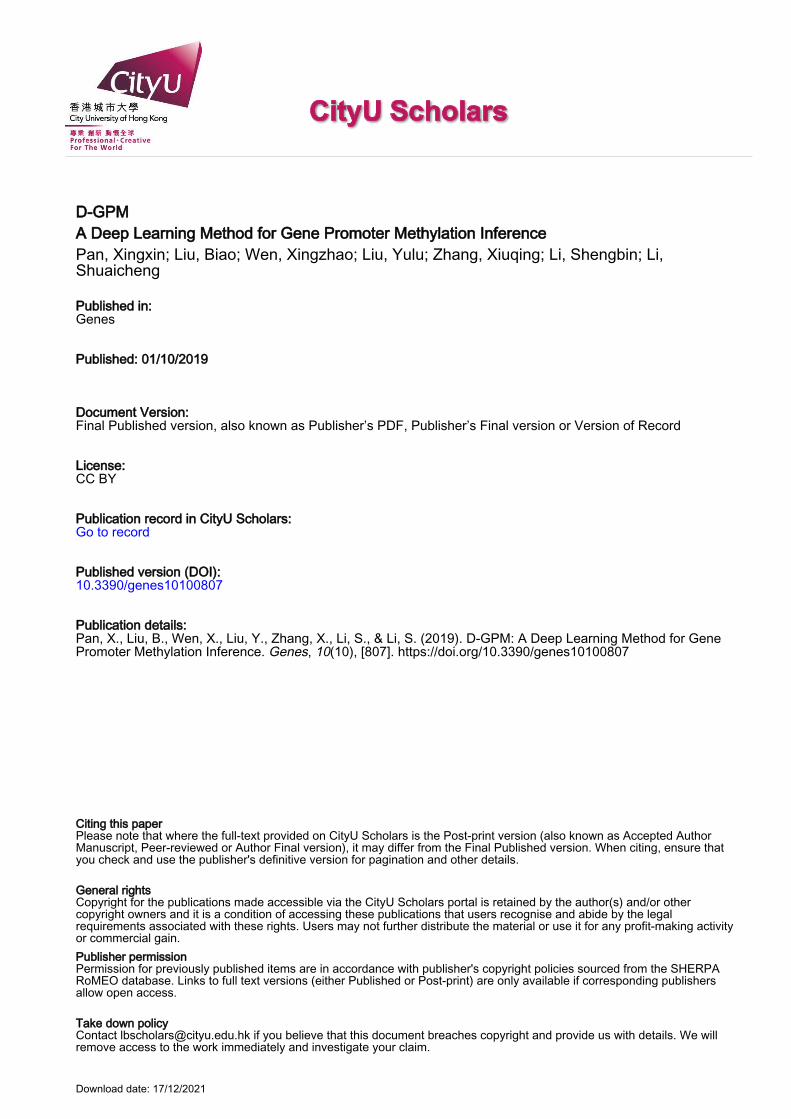
Table 1. Detailed parameter configurations for D-GPM.

Parameters

# of hidden layers [1–8]# of hidden units in each hidden layer [1000,2000,3000,4000,5000,6000,7000,8000,9000]Dropout rate [0%, 5%,1 0%, 15%, 20%, 25%, 30%, 35%, 40%, 45%, 50%]Momentum coefficient 0.5Initial learning rate 5 × 10−4, 2 × 10−4, 1 × 10−4 or 8 × 10−5

Minimum learning rate 1.00 × 10−5

Learning rate decay factor 0.9Learning scale 3.0Mini-batch size 200Training epoch 500

Weights’ initial range[−

√6

√ni+no

,√

6√

ni+no

]

According to the parameter configurations, all the combinations of parameters are made duringthe D-GPM training for predicting the promoter methylation of the target genes.

As Table 2 indicates, D-GPM acquires the best MAE performance for MBV-te, with five hiddenlayers of 7000 units and a 15% dropout rate (D-GPM-15%-7000 × 5) among the 792 (8 × 9 × 11) variousD-GPMs. Meanwhile, D-GPM has an extraordinary edge over MAE compared with LR, SVM, and RT.

Table 2. The mean absolute error (MAE)-based overall errors of linear regression (LR), the regressiontree (RT), the support vector machine (SVM), and D-GPM, with partially different architectures (hiddenlayer: from 4 to 6, with step size 1; hidden unit: from 6000 to 8000, with step size 1000; dropout rate:from 10% to 20%, with step size 5%) for MBV-te. The numbers before “±” are the overall MAE for allthe target genes. The numbers after “±” are the standard deviations of the predicted MAE over all thetarget genes. The best MAE performance of D-GPM is underlined. SD refers to the standard deviation.

Hidden Layers Dropout RateHidden Units

6000 7000 8000

4 10% 0.0332 ± 0.0253 0.0340 ± 0.0260 0.0343 ± 0.02634 15% 0.0333 ± 0.0253 0.0340 ± 0.0260 0.0344 ± 0.02644 20% 0.0336 ± 0.0255 0.0343 ± 0.0261 0.0344 ± 0.02625 10% 0.0344 ± 0.0264 0.0337 ± 0.0257 0.0346 ± 0.02645 15% 0.0343 ± 0.0260 0.0329 ± 0.0251 0.0343 ± 0.02615 20% 0.0350 ± 0.0267 0.0343 ± 0.0259 0.0347 ± 0.02656 10% 0.0341 ± 0.0259 0.0339 ± 0.0258 0.0339 ± 0.02586 15% 0.0339 ± 0.0259 0.0334 ± 0.0255 0.0331 ± 0.02536 20% 0.0356 ± 0.0269 0.0346 ± 0.0261 0.0351 ± 0.0265

Linear regression 0.0363 ± 0.0277

Support vector machine 0.0350 ± 0.0258Regression tree 0.0454 ± 0.0363

Similarly, D-GPM-15%-7000 × 5 also obtains the best PCC performance for MBV-te among the 792prediction models, as shown in Table 3. The complete MAE and PCC evaluation of D-GPM armedwith all the other architectures (hidden layer: from 1 to 8, with step size 1; hidden unit: from 1000 to9000, with step size 1000; dropout rate: from 0% to 50%, with step size 5%) for the MBV-te is given inthe Supplementary Materials.

Genes 2019, 10, 807 8 of 16

Table 3. The Pearson correlation coefficient (PCC) of LR, RT, SVM, and D-GPM, with partially differentarchitectures (hidden layer: from 4 to 6, with step size 1; hidden unit: from 6000 to 8000, with stepsize 1000; dropout rate: from 10% to 20%, with step size 5%) for MBV-te. The numbers before “±”are the overall PCC for all the target genes. The numbers after “±” are the standard deviations of thePCC over all the target genes. The best PCC performance of D-GPM is underlined. SD refers to thestandard deviation.

Hidden Layers Dropout RateHidden Units

6000 7000 8000

4 10% 0.8081 ± 0.0964 0.7972 ± 0.0976 0.8058 ± 0.09574 15% 0.8055 ± 0.0968 0.7936 ± 0.0989 0.8041 ± 0.09614 20% 0.8077 ± 0.0964 0.8032 ± 0.0964 0.7968 ± 0.09515 10% 0.7776 ± 0.1022 0.8032 ± 0.0984 0.7990 ± 0.09445 15% 0.7842 ± 0.1012 0.8186 ± 0.0940 0.7828 ± 0.10355 20% 0.7835 ± 0.1001 0.8135 ± 0.0943 0.7933 ± 0.09976 10% 0.7919 ± 0.0987 0.8007 ± 0.0961 0.8010 ± 0.09476 15% 0.7865 ± 0.1002 0.8086 ± 0.0923 0.8106 ± 0.09146 20% 0.7879 ± 0.1006 0.8082 ± 0.0925 0.7952 ± 0.0975

Linear regression 0.7846 ± 0.1069

Support vector machine 0.7942 ± 0.1056

Regression tree 0.6657 ± 0.1192

Based on the above overall MAE and PCC performance for all the target genes, we can concludethat D-GPM, with five hidden layers of 7000 units and a 15% dropout rate, is the best model forpredicting promoter methylation among the prediction models.

3.2. Evaluation According to MAE Criteria

D-GPM acquires the best overall MAE performance for the MBV-te, with a 15% dropout rate(described as D-GPM-15%) among the eleven dropout rates, ranging from 0% to 50%, with a stepsize of 5%. Figure 3 shows the overall MAE performances of D-GPM-15% for the MBV-te and SVMacts as a benchmark. The larger architecture of D-GPM-15% (five hidden layers with 7000 hiddenunits in each hidden layer, described as D-GPM-15%-7000 × 5) acquires the least MAE for the MBV-te.D-GPM-15%-7000 × 5 outperforms LR by reducing the MAE by 9.59%, RT by reducing the MAEby 27.58% and SVM by reducing the MAE by 6.14%, respectively. A possible explanation for this isthat deep learning models possess much richer representability, capture complex features, and makelearning intrinsic characteristics much easier [31].

D-GPM also outperforms LR and RT for almost all the target genes in terms of the MAE. Figure 4shows the density plots of the MAE of all the target genes by LR, RT, SVM, and D-GPM. On the whole,D-GPM occupies a larger proportion at the low MAE level and a lower proportion at the high MAElevel compared to the three machine learning methods, especially for RT and LR, attesting to theprominent performance of D-GPM.

Figure 5a–c displays a gene-wise comparative analysis of D-GPM and the other three methods.In terms of MAE, D-GPM outperforms RT for 95.66% (20,705 genes) of the target genes, outperformsLR for 92.65% (20,054 genes) of the target genes, and outperforms SVM for 85.49% (18,504 genes) ofthe target genes. These results can also be viewed by the larger proportion of dots that lie above thediagonal, and the better performance may suggest that D-GPM can capture some intrinsic nonlinearfeatures of the MBV data, which LR, RT, and SVM did not accomplish.

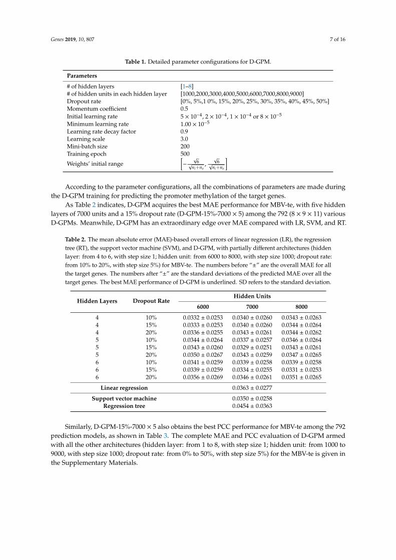
Genes 2019, 10, 807 9 of 16Genes 2019, 10, 807 9 of 16

Figure 3. The overall MAE errors of D-GPM-15%, with various architectures for the MBV-te. The overall MAE errors of SVM for the MBV-te are shown as a cross section, which is 0.0350 high in terms of the MAE and serves as a benchmark to evaluate the MAE of D-GPM-15% with various architectures.

Figure 4. The density plots of the MAE by LR, RT, SVM, and D-GPM for the MBV-te.

Figure 3. The overall MAE errors of D-GPM-15%, with various architectures for the MBV-te. The overallMAE errors of SVM for the MBV-te are shown as a cross section, which is 0.0350 high in terms of theMAE and serves as a benchmark to evaluate the MAE of D-GPM-15% with various architectures.

Genes 2019, 10, 807 9 of 16

Figure 3. The overall MAE errors of D-GPM-15%, with various architectures for the MBV-te. The overall MAE errors of SVM for the MBV-te are shown as a cross section, which is 0.0350 high in terms of the MAE and serves as a benchmark to evaluate the MAE of D-GPM-15% with various architectures.

Figure 4. The density plots of the MAE by LR, RT, SVM, and D-GPM for the MBV-te. Figure 4. The density plots of the MAE by LR, RT, SVM, and D-GPM for the MBV-te.

Genes 2019, 10, 807 10 of 16

Genes 2019, 10, 807 10 of 16

Figure 5. The predictive MAE of each target gene by D-GPM compared with RT, LR, and SVM for MBV-te. Each dot represents one of the 21,645 target genes. The x-axis is the MAE of each target gene obtained by D-GPM, and the y-axis is the MAE of each target gene obtained by the other machine learning method. The dots above the diagonal indicate that D-GPM achieves lower MAE compared with the other method. (a) D-GPM versus RT. (b) D-GPM versus LR. (c) D-GPM versus SVM.

RT performs significantly worse than the other methods in terms of the MAE. One possible reason for this is that the model is too oversimplified to capture the essential features between promoter methylation of the landmark and target genes based on the MBV-te [32].

According to the model distribution of the lowest MAE for each target gene, we found the best model distribution, as shown in Figure 6a. RT accomplishes the best MAE performance for 305 target genes (1.41%), including the genes BRD2, GPI, MAF, and MICB, implying that there is a relatively simple promoter methylation regulation mechanism and promoter methylation of these target genes may be dominantly regulated by a very few specific landmark genes. The LR can predict 1242 target genes (5.74%), at best, among the other three methods, including the genes ABCD1, HPD, AMH, and ARAF, laying a solid foundation for the pathogenesis of diseases, such as Adrenoleukodystrophy, Hawkinsinuria, Persistent Mullerian Duct Syndrome, and Pallister-Killian Syndrome, using our LR [33–36]. Noticeably, SVM performs best for a total of 2813 genes (13.00%), including ACE2, A2M, and CA1. One possible explanation for this is that there seem to be intricate and complicated interactions among the promoter methylation of the landmark genes and these 2813 target genes. Undoubtedly, D-GPM does better than the other three methods, as far as 17,285 target genes (79.86%) are concerned, demonstrating the deep neural networks’ powerful ability to capture the nonlinear relationship of methylation profiling.

Figure 6. Distribution of the best model. (a) Distribution of the best model according to MAE for the target genes. (b) Distribution of best model according to PCC for the target genes.

3.3. Evaluation According to PCC Criteria

D-GPM accomplishes the best overall PCC performance for the MBV-te, with a 15% dropout rate. Figure 7 shows the overall PCC performances of D-GPM-15% and the other methods for MBV-te. Similar to the MAE, D-GPM-15%-7000 × 5 acquires the most significant PCC for the MBV-te. The relative PCC improvement of D-GPM-15%-7000 × 5 is 4.34% compared to the LR, 22.96% compared

Figure 5. The predictive MAE of each target gene by D-GPM compared with RT, LR, and SVM forMBV-te. Each dot represents one of the 21,645 target genes. The x-axis is the MAE of each target geneobtained by D-GPM, and the y-axis is the MAE of each target gene obtained by the other machinelearning method. The dots above the diagonal indicate that D-GPM achieves lower MAE comparedwith the other method. (a) D-GPM versus RT. (b) D-GPM versus LR. (c) D-GPM versus SVM.

RT performs significantly worse than the other methods in terms of the MAE. One possible reasonfor this is that the model is too oversimplified to capture the essential features between promotermethylation of the landmark and target genes based on the MBV-te [32].

According to the model distribution of the lowest MAE for each target gene, we found the bestmodel distribution, as shown in Figure 6a. RT accomplishes the best MAE performance for 305 targetgenes (1.41%), including the genes BRD2, GPI, MAF, and MICB, implying that there is a relativelysimple promoter methylation regulation mechanism and promoter methylation of these target genesmay be dominantly regulated by a very few specific landmark genes. The LR can predict 1242 targetgenes (5.74%), at best, among the other three methods, including the genes ABCD1, HPD, AMH, andARAF, laying a solid foundation for the pathogenesis of diseases, such as Adrenoleukodystrophy,Hawkinsinuria, Persistent Mullerian Duct Syndrome, and Pallister-Killian Syndrome, using ourLR [33–36]. Noticeably, SVM performs best for a total of 2813 genes (13.00%), including ACE2, A2M,and CA1. One possible explanation for this is that there seem to be intricate and complicated interactionsamong the promoter methylation of the landmark genes and these 2813 target genes. Undoubtedly,D-GPM does better than the other three methods, as far as 17,285 target genes (79.86%) are concerned,demonstrating the deep neural networks’ powerful ability to capture the nonlinear relationship ofmethylation profiling.

Genes 2019, 10, 807 10 of 16

Figure 5. The predictive MAE of each target gene by D-GPM compared with RT, LR, and SVM for MBV-te. Each dot represents one of the 21,645 target genes. The x-axis is the MAE of each target gene obtained by D-GPM, and the y-axis is the MAE of each target gene obtained by the other machine learning method. The dots above the diagonal indicate that D-GPM achieves lower MAE compared with the other method. (a) D-GPM versus RT. (b) D-GPM versus LR. (c) D-GPM versus SVM.

RT performs significantly worse than the other methods in terms of the MAE. One possible reason for this is that the model is too oversimplified to capture the essential features between promoter methylation of the landmark and target genes based on the MBV-te [32].

According to the model distribution of the lowest MAE for each target gene, we found the best model distribution, as shown in Figure 6a. RT accomplishes the best MAE performance for 305 target genes (1.41%), including the genes BRD2, GPI, MAF, and MICB, implying that there is a relatively simple promoter methylation regulation mechanism and promoter methylation of these target genes may be dominantly regulated by a very few specific landmark genes. The LR can predict 1242 target genes (5.74%), at best, among the other three methods, including the genes ABCD1, HPD, AMH, and ARAF, laying a solid foundation for the pathogenesis of diseases, such as Adrenoleukodystrophy, Hawkinsinuria, Persistent Mullerian Duct Syndrome, and Pallister-Killian Syndrome, using our LR [33–36]. Noticeably, SVM performs best for a total of 2813 genes (13.00%), including ACE2, A2M, and CA1. One possible explanation for this is that there seem to be intricate and complicated interactions among the promoter methylation of the landmark genes and these 2813 target genes. Undoubtedly, D-GPM does better than the other three methods, as far as 17,285 target genes (79.86%) are concerned, demonstrating the deep neural networks’ powerful ability to capture the nonlinear relationship of methylation profiling.

Figure 6. Distribution of the best model. (a) Distribution of the best model according to MAE for the target genes. (b) Distribution of best model according to PCC for the target genes.

3.3. Evaluation According to PCC Criteria

D-GPM accomplishes the best overall PCC performance for the MBV-te, with a 15% dropout rate. Figure 7 shows the overall PCC performances of D-GPM-15% and the other methods for MBV-te. Similar to the MAE, D-GPM-15%-7000 × 5 acquires the most significant PCC for the MBV-te. The relative PCC improvement of D-GPM-15%-7000 × 5 is 4.34% compared to the LR, 22.96% compared

Figure 6. Distribution of the best model. (a) Distribution of the best model according to MAE for thetarget genes. (b) Distribution of best model according to PCC for the target genes.

3.3. Evaluation According to PCC Criteria

D-GPM accomplishes the best overall PCC performance for the MBV-te, with a 15% dropoutrate. Figure 7 shows the overall PCC performances of D-GPM-15% and the other methods for MBV-te.Similar to the MAE, D-GPM-15%-7000× 5 acquires the most significant PCC for the MBV-te. The relativePCC improvement of D-GPM-15%-7000 × 5 is 4.34% compared to the LR, 22.96% compared to RT, and

Genes 2019, 10, 807 11 of 16

3.07% compared to SVM. Similar to the MAE, almost all the combined architectures of D-GPM-15%outperform LR and RT in terms of the PCC performance.

Genes 2019, 10, 807 11 of 16

to RT, and 3.07% compared to SVM. Similar to the MAE, almost all the combined architectures of D-GPM-15% outperform LR and RT in terms of the PCC performance.

Figure 7. The overall PCC performance of D-GPM-15% with various architectures for the MBV-te. The overall PCC performance of SVM for the MBV-te is shown as a cross section, which is 0.794183 high in terms of the PCC and serves as a benchmark to evaluate the PCC of D-GPM-15% with various architectures.

In terms of the PCC, D-GPM also outperforms RT and LR for almost all the target genes. Figure 8 displays the density plots of the PCC of all the target genes by LR, RT, SVM, and D-GPM. By and large, we can see that D-GPM possesses a larger proportion at the high PCC level and a lower proportion at the low PCC level compared to the RT, LR, and SVM.

Figure 8. The density plots of the PCC of all the target genes by LR, RT, SVM, and D-GPM for MBV-te.

Figure 7. The overall PCC performance of D-GPM-15% with various architectures for the MBV-te.The overall PCC performance of SVM for the MBV-te is shown as a cross section, which is 0.794183high in terms of the PCC and serves as a benchmark to evaluate the PCC of D-GPM-15% withvarious architectures.

In terms of the PCC, D-GPM also outperforms RT and LR for almost all the target genes. Figure 8displays the density plots of the PCC of all the target genes by LR, RT, SVM, and D-GPM. By and large,we can see that D-GPM possesses a larger proportion at the high PCC level and a lower proportion atthe low PCC level compared to the RT, LR, and SVM.

Genes 2019, 10, 807 11 of 16

to RT, and 3.07% compared to SVM. Similar to the MAE, almost all the combined architectures of D-GPM-15% outperform LR and RT in terms of the PCC performance.

Figure 7. The overall PCC performance of D-GPM-15% with various architectures for the MBV-te. The overall PCC performance of SVM for the MBV-te is shown as a cross section, which is 0.794183 high in terms of the PCC and serves as a benchmark to evaluate the PCC of D-GPM-15% with various architectures.

In terms of the PCC, D-GPM also outperforms RT and LR for almost all the target genes. Figure 8 displays the density plots of the PCC of all the target genes by LR, RT, SVM, and D-GPM. By and large, we can see that D-GPM possesses a larger proportion at the high PCC level and a lower proportion at the low PCC level compared to the RT, LR, and SVM.

Figure 8. The density plots of the PCC of all the target genes by LR, RT, SVM, and D-GPM for MBV-te. Figure 8. The density plots of the PCC of all the target genes by LR, RT, SVM, and D-GPM for MBV-te.

Genes 2019, 10, 807 12 of 16

Figure 9a–c shows a gene-wise comparative analysis of D-GPM and the other three methods.For PCC, D-GPM outperforms RT in 98.25% (21,266 genes) of the target genes, LR in 91.00% (19,696 genes)of the target genes, and SVM in 81.56% (17,653 genes) of the target genes. Therefore, D-GPM’s powerfulpredictive performance for the PCC of all the target genes is preserved, similar to its effective predictionfor the MAE. It is obvious that although the prediction property of the SVM is still modest in terms ofthe PCC, its predictive PCC performance for a number of the target genes is significantly higher thanD-GPM. This finding is probably due to the fact that SVM is based on the principle of structural riskminimization, avoiding overlearning problems, and having a strong generalization ability.

Genes 2019, 10, 807 12 of 16

Figure 9a–c shows a gene-wise comparative analysis of D-GPM and the other three methods. For PCC, D-GPM outperforms RT in 98.25% (21,266 genes) of the target genes, LR in 91.00% (19,696 genes) of the target genes, and SVM in 81.56% (17,653 genes) of the target genes. Therefore, D-GPM’s powerful predictive performance for the PCC of all the target genes is preserved, similar to its effective prediction for the MAE. It is obvious that although the prediction property of the SVM is still modest in terms of the PCC, its predictive PCC performance for a number of the target genes is significantly higher than D-GPM. This finding is probably due to the fact that SVM is based on the principle of structural risk minimization, avoiding overlearning problems, and having a strong generalization ability.

Figure 9. The predictive PCC of each target gene by D-GPM compared with RT, LR, and SVM for MBV-te. Each dot represents one out of the 21,645 target genes. The x-axis is the PCC of each target gene obtained by the above-mentioned three machine learning techniques, and the y-axis is the PCC of each target gene obtained by D-GPM. The dots above the diagonal indicate that D-GPM achieves a higher PCC value compared with the other method. (a) D-GPM versus RT. (b) D-GPM versus LR. (c) D-GPM versus SVM.

According to the model distribution of the maximal PCC for each target gene, we found the best model distribution, as shown in Figure 6b. Surprisingly, RT only obtains the best PCC performance for 19 target genes (0.09%), including the genes ALG1 and NBR2, falling far below the best 305 target genes in terms of the MAE. Considering RT’s awful predictive power for the PCC performance compared with its better predictive power for the MAE performance, this may be explained by the fact that RT makes decisions based on an oversimple assumption. LR predicts the best 1057 target genes (4.88%) among the other three methods, including the genes AASS and ACE, and the proportion of the best target genes of LR in the PCC level is similar to that in the MAE level. For the PCC, SVM is on its best behavior for a total of 3613 target genes (16.69%), having an increasing number compared to that of the MAE, in contrast to RT. Undoubtedly, D-GPM outperforms the other three methods, with regard to 16,956 genes (78.34%), in terms of the PCC.

Noticeably, the dropout regularization manages to improve the performance of D-GPM-15%-7000 × 5 for the MBV-te, as shown in Figure 10. With a 15% dropout rate, D-GPM-15%-7000 × 5 consistently achieves the best MAE performance for the MBV-te among the models, with 0%, 15%, 20%, 25%, and 35% dropout rates.

Figure 9. The predictive PCC of each target gene by D-GPM compared with RT, LR, and SVM forMBV-te. Each dot represents one out of the 21,645 target genes. The x-axis is the PCC of each targetgene obtained by the above-mentioned three machine learning techniques, and the y-axis is the PCCof each target gene obtained by D-GPM. The dots above the diagonal indicate that D-GPM achievesa higher PCC value compared with the other method. (a) D-GPM versus RT. (b) D-GPM versus LR.(c) D-GPM versus SVM.

According to the model distribution of the maximal PCC for each target gene, we found the bestmodel distribution, as shown in Figure 6b. Surprisingly, RT only obtains the best PCC performance for19 target genes (0.09%), including the genes ALG1 and NBR2, falling far below the best 305 target genesin terms of the MAE. Considering RT’s awful predictive power for the PCC performance comparedwith its better predictive power for the MAE performance, this may be explained by the fact that RTmakes decisions based on an oversimple assumption. LR predicts the best 1057 target genes (4.88%)among the other three methods, including the genes AASS and ACE, and the proportion of the besttarget genes of LR in the PCC level is similar to that in the MAE level. For the PCC, SVM is on its bestbehavior for a total of 3613 target genes (16.69%), having an increasing number compared to that of theMAE, in contrast to RT. Undoubtedly, D-GPM outperforms the other three methods, with regard to16,956 genes (78.34%), in terms of the PCC.

Noticeably, the dropout regularization manages to improve the performance of D-GPM-15%-7000× 5 for the MBV-te, as shown in Figure 10. With a 15% dropout rate, D-GPM-15%-7000 × 5 consistentlyachieves the best MAE performance for the MBV-te among the models, with 0%, 15%, 20%, 25%, and35% dropout rates.

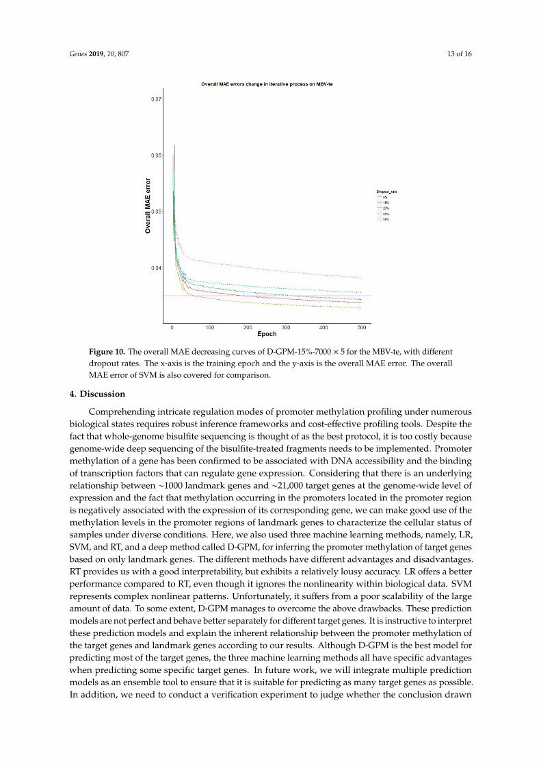
Genes 2019, 10, 807 13 of 16Genes 2019, 10, 807 13 of 16

Figure 10. The overall MAE decreasing curves of D-GPM-15%-7000 × 5 for the MBV-te, with different dropout rates. The x-axis is the training epoch and the y-axis is the overall MAE error. The overall MAE error of SVM is also covered for comparison.

4. Discussion

Comprehending intricate regulation modes of promoter methylation profiling under numerous biological states requires robust inference frameworks and cost-effective profiling tools. Despite the fact that whole-genome bisulfite sequencing is thought of as the best protocol, it is too costly because genome-wide deep sequencing of the bisulfite-treated fragments needs to be implemented. Promoter methylation of a gene has been confirmed to be associated with DNA accessibility and the binding of transcription factors that can regulate gene expression. Considering that there is an underlying relationship between ∼1000 landmark genes and ∼21,000 target genes at the genome-wide level of expression and the fact that methylation occurring in the promoters located in the promoter region is negatively associated with the expression of its corresponding gene, we can make good use of the methylation levels in the promoter regions of landmark genes to characterize the cellular status of samples under diverse conditions. Here, we also used three machine learning methods, namely, LR, SVM, and RT, and a deep method called D-GPM, for inferring the promoter methylation of target genes based on only landmark genes. The different methods have different advantages and disadvantages. RT provides us with a good interpretability, but exhibits a relatively lousy accuracy. LR offers a better performance compared to RT, even though it ignores the nonlinearity within biological data. SVM represents complex nonlinear patterns. Unfortunately, it suffers from a poor scalability of the large amount of data. To some extent, D-GPM manages to overcome the above drawbacks. These prediction models are not perfect and behave better separately for different target genes. It is instructive to interpret these prediction models and explain the inherent relationship between the promoter methylation of the target genes and landmark genes according to our results. Although D-GPM is the best model for predicting most of the target genes, the three machine learning methods all have specific advantages when predicting some specific target genes. In future work, we will integrate multiple prediction models as an ensemble tool to ensure that it is suitable for predicting as many target genes as possible. In addition, we need to conduct a verification experiment to judge whether the conclusion drawn from the relationship between the promoter methylation of the target and landmark genes (such as TDP1 and CIAPIN1) is sound and persuasive. Furthermore,

Figure 10. The overall MAE decreasing curves of D-GPM-15%-7000 × 5 for the MBV-te, with differentdropout rates. The x-axis is the training epoch and the y-axis is the overall MAE error. The overallMAE error of SVM is also covered for comparison.

4. Discussion

Comprehending intricate regulation modes of promoter methylation profiling under numerousbiological states requires robust inference frameworks and cost-effective profiling tools. Despite thefact that whole-genome bisulfite sequencing is thought of as the best protocol, it is too costly becausegenome-wide deep sequencing of the bisulfite-treated fragments needs to be implemented. Promotermethylation of a gene has been confirmed to be associated with DNA accessibility and the bindingof transcription factors that can regulate gene expression. Considering that there is an underlyingrelationship between ∼1000 landmark genes and ∼21,000 target genes at the genome-wide level ofexpression and the fact that methylation occurring in the promoters located in the promoter regionis negatively associated with the expression of its corresponding gene, we can make good use of themethylation levels in the promoter regions of landmark genes to characterize the cellular status ofsamples under diverse conditions. Here, we also used three machine learning methods, namely, LR,SVM, and RT, and a deep method called D-GPM, for inferring the promoter methylation of target genesbased on only landmark genes. The different methods have different advantages and disadvantages.RT provides us with a good interpretability, but exhibits a relatively lousy accuracy. LR offers a betterperformance compared to RT, even though it ignores the nonlinearity within biological data. SVMrepresents complex nonlinear patterns. Unfortunately, it suffers from a poor scalability of the largeamount of data. To some extent, D-GPM manages to overcome the above drawbacks. These predictionmodels are not perfect and behave better separately for different target genes. It is instructive to interpretthese prediction models and explain the inherent relationship between the promoter methylation ofthe target genes and landmark genes according to our results. Although D-GPM is the best model forpredicting most of the target genes, the three machine learning methods all have specific advantageswhen predicting some specific target genes. In future work, we will integrate multiple predictionmodels as an ensemble tool to ensure that it is suitable for predicting as many target genes as possible.In addition, we need to conduct a verification experiment to judge whether the conclusion drawn

Genes 2019, 10, 807 14 of 16

from the relationship between the promoter methylation of the target and landmark genes (such asTDP1 and CIAPIN1) is sound and persuasive. Furthermore, after obtaining the ensemble predictionmodel, we will make the most of it to impute and revise methylation sites that are missing or have alow reliability in realistic methylation profiling data.

5. Conclusions

In summary, D-GPM acquires the least overall MAE and the highest PCC for the MBV-te amongLR, RT, and SVM. For a gene-wise comparative analysis of D-GPM and the above three methods,D-GPM outperforms LR, RT, and SVM for predicting an overwhelming majority of the target genes,concerning the MAE and PCC. In addition, according to the model distribution of the least MAE andthe highest PCC for the target genes, D-GPM predominates among the other models for predicting amajority of the target genes, laying a solid foundation for explaining the inherent relationship betweenthe promoter methylation of target genes and landmark genes via interpreting results from theseprediction models.

Supplementary Materials: The following are available online at http://www.mdpi.com/2073-4425/10/10/807/s1:The complete MAE and PCC evaluation of D-GPM armed with all the other architectures (hidden layer: from1 to 8, with step size 1; hidden unit: from 1000 to 9000, with step size 1000; dropout rate: from 0% to 50%, withstep size 5%) for the MBV-te is given in the file named “The complete evaluation.txt”.

Author Contributions: Conceptualization, X.P. and S.L. (Shuaicheng Li); data curation, B.L. and Y.L.; formalanalysis, X.P. and B.L.; investigation, X.P., B.L., X.W., Y.L., X.Z., S.L. (Shengbin Li).; methodology, X.P.; projectadministration, X.P.; resources, B.L.; software, X.P. and B.L.; supervision, X.Z. and S.L. (Shuaicheng Li); validation,X.P.; visualization, X.P. and X.W.; writing—original draft, X.P. and X.W.; writing—review and editing, X.P.,B.L., X.W.

Funding: This research received no external funding.

Acknowledgments: The authors acknowledge BGI-Shenzhen for the computing resources and the TCGA projectorganizers for the public datasets.

Conflicts of Interest: The authors declare no conflicts of interest.

References

1. Moore, L.D.; Le, T.; Fan, G. DNA methylation and its basic function. Neuropsychopharmacol. Off. Publ. Am.Coll. Neuropsychopharmacol. 2013, 38, 23. [CrossRef] [PubMed]

2. Jones, P.A. Functions of DNA methylation: Islands, start sites, gene bodies and beyond. Nat. Rev. Genet.2012, 13, 484–492. [CrossRef] [PubMed]

3. Bird, A. DNA methylation patterns and epigenetic memory. Genes Dev. 2002, 16, 6–21. [CrossRef] [PubMed]4. Bestor, T.H.; Edwards, J.R.; Boulard, M. Notes on the role of dynamic DNA methylation in mammalian

development. Proc. Natl. Acad. Sci. USA 2015, 112, 6796–6799. [CrossRef]5. Huang, Y.-W.; Huang, T.H.-M.; Wang, L.-S. Profiling DNA methylomes from microarray to genome-scale

sequencing. Technol. Cancer Res. Treat. 2010, 9, 139–147. [CrossRef]6. Laird, P.W. Principles and challenges of genome-wide DNA methylation analysis. Nat. Rev. Genet. 2010,

11, 191–203. [CrossRef]7. Plongthongkum, N.; Diep, D.H.; Zhang, K. Advances in the profiling of DNA modifications: Cytosine

methylation and beyond. Nat. Rev. Genet. 2014, 15, 647–661. [CrossRef]8. Schwartzman, O.; Tanay, A. Single-cell epigenomics: Techniques and emerging applications. Nat. Rev. Genet.

2015, 16, 716–726. [CrossRef]9. Krygier, M.; Podolak-Popinigis, J.; Limon, J.; Sachadyn, P.; Stanislawska-Sachadyn, A. A simple modification

to improve the accuracy of methylation-sensitive restriction enzyme quantitative polymerase chain reaction.Anal. Biochem. 2016, 500, 88–90. [CrossRef]

10. Thu, K.L.; Vucic, E.A.; Kennett, J.Y.; Heryet, C.; Brown, C.J.; Lam, W.L.; Wilson, I.M. Methylated DNAimmunoprecipitation. J. Vis. Exp. 2009, 23, 935. [CrossRef]

11. Bibikova, M.; Le, J.; Barnes, B.; Saedinia-Melnyk, S.; Zhou, L.; Shen, R.; Gunderson, K.L. Genome-wide DNAmethylation profiling using Infinium(R) assay. Epigenomics 2009, 1, 177–200. [CrossRef] [PubMed]

Genes 2019, 10, 807 15 of 16

12. Li, Q.; Hermanson, P.J.; Springer, N.M. Detection of DNA Methylation by Whole-Genome Bisulfite Sequencing.Methods Mol. Biol. (Clifton N.J.) 2018, 1676, 185–196. [CrossRef]

13. Chen, Y.; Li, Y.; Narayan, R.; Subramanian, A.; Xie, X. Gene expression inference with deep learning.Bioinformatics 2016, 32, 1832–1839. [CrossRef] [PubMed]

14. Bansal, M.; Belcastro, V.; Ambesi-Impiombato, A.; di Bernardo, D. How to infer gene networks fromexpression profiles. Mol. Syst. Biol. 2007, 3, 78. [CrossRef]

15. Edgar, R.; Domrachev, M.; Lash, A.E. Gene Expression Omnibus: NCBI gene expression and hybridizationarray data repository. Nucleic Acids Res. 2002, 30, 207–210. [CrossRef]

16. Medvedeva, Y.A.; Khamis, A.M.; Kulakovskiy, I.V.; Ba-Alawi, W.; Bhuyan, M.S.I.; Kawaji, H.; Lassmann, T.;Harbers, M.; Forrest, A.R.; Bajic, V.B. Effects of cytosine methylation on transcription factor binding sites.BMC Genom. 2014, 15, 119. [CrossRef]

17. Xiong, H.Y.; Alipanahi, B.; Lee, L.J.; Bretschneider, H.; Merico, D.; Yuen, R.K.; Hua, Y.; Gueroussov, S.;Najafabadi, H.S.; Hughes, T.R. The human splicing code reveals new insights into the genetic determinantsof disease. Science 2015, 347, 1254806. [CrossRef]

18. Kelley, D.R.; Snoek, J.; Rinn, J.L. Basset: Learning the regulatory code of the accessible genome with deepconvolutional neural networks. Genome Res. 2016, 26, 990–999. [CrossRef]

19. Zhou, J.; Troyanskaya, O.G. Predicting effects of noncoding variants with deep learning–based sequencemodel. Nat. Methods 2015, 12, 931–934. [CrossRef]

20. Tomczak, K.; Czerwinska, P.; Wiznerowicz, M. The Cancer Genome Atlas (TCGA): An immeasurable sourceof knowledge. Contemp. Oncol. (Poznan Poland) 2015, 19, A68–A77. [CrossRef]

21. Touleimat, N.; Tost, J. Complete pipeline for Infinium((R)) Human Methylation 450K BeadChip dataprocessing using subset quantile normalization for accurate DNA methylation estimation. Epigenomics 2012,4, 325–341. [CrossRef] [PubMed]

22. Huang, W.Y.; Hsu, S.D.; Huang, H.Y.; Sun, Y.M.; Chou, C.H.; Weng, S.L.; Huang, H.D. MethHC: A database ofDNA methylation and gene expression in human cancer. Nucleic Acids Res. 2015, 43, D856–D861. [CrossRef][PubMed]

23. Srivastava, N.; Hinton, G.; Krizhevsky, A.; Sutskever, I.; Salakhutdinov, R. Dropout: A simple way to preventneural networks from overfitting. J. Mach. Learn. Res. 2014, 15, 1929–1958.

24. Sutskever, I.; Martens, J.; Dahl, G.; Hinton, G. On the importance of initialization and momentum in deeplearning. In Proceedings of the International Conference on Machine Learning, Atlanta, GA, USA, 16–21June 2013; pp. 1139–1147.

25. Goodfellow, I.J.; Wardefarley, D.; Lamblin, P.; Dumoulin, V.; Mirza, M.; Pascanu, R.; Bergstra, J.; Bastien, F.;Bengio, Y. Pylearn2: A machine learning research library. arXiv 2013, arXiv:1308.4214.

26. Bergstra, J.; Breuleux, O.; Bastien, F.; Lamblin, P.; Pascanu, R.; Desjardins, G.; Turian, J.; Warde-Farley, D.;Bengio, Y. Theano: A CPU and GPU math expression compiler. In Proceedings of the Python for ScientificComputing Conference (SciPy), Austin, TX, USA, 28 June 28–3 July 2010.

27. Therneau, T.; Atkinson, B.; Ripley, B. Package ‘rpart’. 2015. Available online: cran.ma.ic.ac.uk/web/packages/rpart/rpart.pdf (accessed on 20 April 2016).

28. Steinwart, I.; Hush, D.; Scovel, C. An Explicit Description of the Reproducing Kernel Hilbert Spaces ofGaussian RBF Kernels. IEEE Trans. Inf. Theory 2006, 52, 4635–4643. [CrossRef]

29. Karatzoglou, A.; Smola, A.; Hornik, K.; Zeileis, A. kernlab—An S4 Package for Kernel Methods in R. J. Stat.Softw. 2004, 11, 721–729. [CrossRef]

30. Hinton, G.E.; Srivastava, N.; Krizhevsky, A.; Sutskever, I.; Salakhutdinov, R.R. Improving neural networksby preventing co-adaptation of feature detectors. Comput. Sci. 2012, 3, 212–223.

31. Glorot, X.; Bengio, Y. Understanding the difficulty of training deep feedforward neural networks. J. Mach.Learn. Res. 2010, 9, 249–256.

32. Lewis, R.J. An introduction to classification and regression tree (CART) analysis. In Proceedings of theAnnual Meeting of the Society for Academic Emergency Medicine, San Francisco, CA, USA, 22–25 May 2000.

33. Park, J.A.; Jun, K.R.; Han, S.H.; Kim, G.H.; Yoo, H.W.; Hur, Y.J. A novel mutation in the ABCD1 gene of aKorean boy diagnosed with X-linked adrenoleukodystrophy. Gene 2012, 498, 131–133. [CrossRef]

34. Thodi, G.; Schulpis, K.H.; Dotsikas, Y.; Pavlides, C.; Molou, E.; Chatzidaki, M.; Triantafylli, O.; Loukas, Y.L.Hawkinsinuria in two unrelated Greek newborns: Identification of a novel variant, biochemical findings andtreatment. J. Pediatr. Endocrinol. Metab. JPEM 2016, 29, 15–20. [CrossRef]

Genes 2019, 10, 807 16 of 16

35. Wongprasert, H.; Somanunt, S.; De Filippo, R.; Picard, J.Y.; Pitukcheewanont, P. A novel mutation ofanti-Mullerian hormone gene in Persistent Mullerian Duct Syndrome presented with bilateral cryptorchidism:A case report. J. Pediatr. Urol. 2013, 9, e147–e149. [CrossRef] [PubMed]

36. Ticho, B.H. Iris transillumination defects associated with pallister-killian syndrome. J. Pediatr. Ophthalmol.Strabismus 2010, 47, 58–59. [CrossRef] [PubMed]

© 2019 by the authors. Licensee MDPI, Basel, Switzerland. This article is an open accessarticle distributed under the terms and conditions of the Creative Commons Attribution(CC BY) license (http://creativecommons.org/licenses/by/4.0/).