arX

iv:h

ep-t

h/04

0316

6v1

16

Mar

200

4DUKE-CGTP-04-04hep-th/0403166

March 2004

D-Branes on Calabi–Yau Manifolds

Paul S. Aspinwall

Center for Geometry and Theoretical Physics

Box 90318

Duke University

Durham, NC 27708-0318

Abstract

In this review we study BPS D-branes on Calabi–Yau threefolds. Such D-branesnaturally divide into two sets called A-branes and B-branes which are most easilyunderstood from topological field theory. The main aim of this paper is to providea self-contained guide to the derived category approach to B-branes and the idea ofΠ-stability. We argue that this mathematical machinery is hard to avoid for a properunderstanding of B-branes. A-branes and B-branes are related in a very complicatedand interesting way which ties in with the “homological mirror symmetry” conjectureof Kontsevich. We motivate and exploit this form of mirror symmetry. The examplesof the quintic 3-fold, flops and orbifolds are discussed at some length. In the lattercase we describe the role of McKay quivers in the context of D-branes.

Contents

1 Introduction 3

2 Worldsheet Models of Closed Strings 4

2.1 The N = (2, 2) non-linear σ-model . . . . . . . . . . . . . . . . . . . . . . . 42.2 The A model . . . . . . . . . . . . . . . . . . . . . . . . . . . . . . . . . . . 72.3 The B model . . . . . . . . . . . . . . . . . . . . . . . . . . . . . . . . . . . 122.4 Mirror Symmetry . . . . . . . . . . . . . . . . . . . . . . . . . . . . . . . . . 13

3 Boundaries 17

3.1 The A-model . . . . . . . . . . . . . . . . . . . . . . . . . . . . . . . . . . . 173.1.1 A-branes . . . . . . . . . . . . . . . . . . . . . . . . . . . . . . . . . . 173.1.2 Open strings for one A-brane . . . . . . . . . . . . . . . . . . . . . . 203.1.3 Open strings for many A-branes . . . . . . . . . . . . . . . . . . . . . 23

3.2 The B-model . . . . . . . . . . . . . . . . . . . . . . . . . . . . . . . . . . . 283.2.1 B-branes . . . . . . . . . . . . . . . . . . . . . . . . . . . . . . . . . . 283.2.2 Open strings for B-branes . . . . . . . . . . . . . . . . . . . . . . . . 293.2.3 A failure of mirror symmetry . . . . . . . . . . . . . . . . . . . . . . 30

4 Some Mathematical Tools 30

4.1 Categories of sheaves . . . . . . . . . . . . . . . . . . . . . . . . . . . . . . . 314.1.1 Holomorphic functions . . . . . . . . . . . . . . . . . . . . . . . . . . 314.1.2 Sheaves . . . . . . . . . . . . . . . . . . . . . . . . . . . . . . . . . . 314.1.3 Locally free sheaves . . . . . . . . . . . . . . . . . . . . . . . . . . . . 334.1.4 Kernels and cokernels . . . . . . . . . . . . . . . . . . . . . . . . . . . 344.1.5 Abelian categories . . . . . . . . . . . . . . . . . . . . . . . . . . . . 364.1.6 Coherent sheaves . . . . . . . . . . . . . . . . . . . . . . . . . . . . . 38

4.2 Cohomology . . . . . . . . . . . . . . . . . . . . . . . . . . . . . . . . . . . . 394.2.1 Cech cohomology . . . . . . . . . . . . . . . . . . . . . . . . . . . . . 394.2.2 Spectral sequences . . . . . . . . . . . . . . . . . . . . . . . . . . . . 414.2.3 Dolbeault cohomology . . . . . . . . . . . . . . . . . . . . . . . . . . 424.2.4 Sheaf cohomology . . . . . . . . . . . . . . . . . . . . . . . . . . . . . 44

5 The Category of B-branes 48

5.1 Deformations and complexes . . . . . . . . . . . . . . . . . . . . . . . . . . . 485.2 Open strings . . . . . . . . . . . . . . . . . . . . . . . . . . . . . . . . . . . . 505.3 The derived category . . . . . . . . . . . . . . . . . . . . . . . . . . . . . . . 535.4 Coherent sheaves . . . . . . . . . . . . . . . . . . . . . . . . . . . . . . . . . 565.5 More deformations . . . . . . . . . . . . . . . . . . . . . . . . . . . . . . . . 575.6 Anti-branes and K-Theory . . . . . . . . . . . . . . . . . . . . . . . . . . . . 595.7 Mirror symmetry restored? . . . . . . . . . . . . . . . . . . . . . . . . . . . . 61

1

6 Stability 63

6.1 A-Branes . . . . . . . . . . . . . . . . . . . . . . . . . . . . . . . . . . . . . . 636.1.1 Special Lagrangians . . . . . . . . . . . . . . . . . . . . . . . . . . . . 636.1.2 A geometrical decay . . . . . . . . . . . . . . . . . . . . . . . . . . . 656.1.3 Tachyon condensates . . . . . . . . . . . . . . . . . . . . . . . . . . . 69

6.2 B-Branes . . . . . . . . . . . . . . . . . . . . . . . . . . . . . . . . . . . . . . 706.2.1 Triangles . . . . . . . . . . . . . . . . . . . . . . . . . . . . . . . . . . 716.2.2 Categorical mirror symmetry at last . . . . . . . . . . . . . . . . . . . 756.2.3 Π-Stability . . . . . . . . . . . . . . . . . . . . . . . . . . . . . . . . . 766.2.4 Multiple decays . . . . . . . . . . . . . . . . . . . . . . . . . . . . . . 786.2.5 µ-stability . . . . . . . . . . . . . . . . . . . . . . . . . . . . . . . . . 80

7 Applications 83

7.1 The Quintic Threefold . . . . . . . . . . . . . . . . . . . . . . . . . . . . . . 837.1.1 Periods . . . . . . . . . . . . . . . . . . . . . . . . . . . . . . . . . . . 847.1.2 4-branes . . . . . . . . . . . . . . . . . . . . . . . . . . . . . . . . . . 867.1.3 Exotic B-branes . . . . . . . . . . . . . . . . . . . . . . . . . . . . . . 887.1.4 Monodromy . . . . . . . . . . . . . . . . . . . . . . . . . . . . . . . . 90

7.2 Flops . . . . . . . . . . . . . . . . . . . . . . . . . . . . . . . . . . . . . . . . 977.3 Orbifolds . . . . . . . . . . . . . . . . . . . . . . . . . . . . . . . . . . . . . . 100

7.3.1 The McKay correspondence . . . . . . . . . . . . . . . . . . . . . . . 1017.3.2 The Douglas–Moore construction . . . . . . . . . . . . . . . . . . . . 1047.3.3 θ-stability . . . . . . . . . . . . . . . . . . . . . . . . . . . . . . . . . 1077.3.4 Periods . . . . . . . . . . . . . . . . . . . . . . . . . . . . . . . . . . . 1097.3.5 Monodromy . . . . . . . . . . . . . . . . . . . . . . . . . . . . . . . . 1127.3.6 Examples of stability . . . . . . . . . . . . . . . . . . . . . . . . . . . 114

8 Conclusion 119

2

1 Introduction

There can be no doubt that the most important development in string theory in recent yearsis the discovery of D-branes. In flat spacetime a D-brane is regarded as a subspace on whichopen strings may end.1 Since string theory modifies classical notions of geometry at shortdistances, it is natural to assume that such a simple picture of a D-brane as a subspace istoo naıve for more general backgrounds. A more abstract notion of a D-brane is required,one which coincides with the notion of a subspace when viewed in the context of only largedistances. The aim of these lectures is to study how this can happen.

It is probably of profound importance in string theory to know a robust definition ofD-branes in the most general space-time background, but this problem is far too difficultwith our present understanding of string theory. Instead we look for the simplest context inwhich one might observe nontrivial D-brane behaviour. We render our model as simple aspossible by the following steps:

1. Get rid of the enormous complications introduced by time by using a compactificationmodel. We will assume our string theory has a target space R1,3×X for some compactspace X. We focus our attention on X.

2. Send the string coupling gs to zero and consider only quantum corrections arising fromnonzero α′ effects.

3. Use just as much supersymmetry as we can while keeping the problem nontrivial.This amounts to an N = (2, 2) supersymmetric theory on the worldsheet with X aCalabi–Yau threefold.

4. Consider only the “topological sector” of the worldsheet theory. This results in afinite-dimensional Hilbert space of open strings and we remove all oscillator modes.

As we will see, after such dramatic simplifications, a very rich model remains which requiressophisticated mathematical tools to analyze. One can only wonder at how abstruse a morerealistic D-brane, with the above assumptions removed, must be!

Much has already been written about D-branes. We refer to [2], for example, for a reviewof many aspects of D-branes. In this paper we chart a slightly different course to usual toachieve our aims. Firstly we try wherever possible to avoid the D-brane world-volumeapproach since this assumes that the D-brane really is a subspace of the target spacetime.Our ideas are then planted on the worldsheet which forces us to take the string couplingto zero. Having put ourselves in the worldsheet, we will avoid much of the boundary-stateformalism that one often employs here. Whether this is a judicious choice is up to the readerto decide, but it does not seem to be of great importance in the context of our discussions.

By restricting attention to the topological sector of N = (2, 2) worldsheet theories weare in the land of mirror symmetry. In order to keep these lecture notes a manageable

1The first reference to such objects that the author is aware of is, oddly enough, section 4 of [1].

3

length we will have to assume at least some familiarity with mirror symmetry for closedstrings. We refer to the TASI 1996 lectures, and in particular [3], for a review. The moremathematical reader is referred to [4]. We will assume a rudimentary knowledge of thegeometry of Calabi–Yau manifolds. The reviews [3, 5] should suffice.

These lectures are primarily intended to review the ideas of the derived category and Π-stability for B-branes. These subjects have been reviewed by Douglas in [6] from a somewhatdifferent direction than we employ here. Douglas also has a shorter, more mathematically-oriented review in the ICM proceedings [7]. In order to motivate and better understandour constructions, a good deal of our discussion will also involve mirror symmetry for openstrings. This latter topic has been extensively studied and reviewed in many places. Inparticular, the reader can consult [8] and references therein for a very detailed review ofmost of the aspects of the subject.

In section 2 we review the basic ideas one needs from topological field theory in thecontext of closed strings. This leads into mirror symmetry which will be a central tool inour analysis. Section 3 is then a guide to adding boundaries to the string worldsheet. Bythe end of this section we will realize that there are some difficulties in maintaining mirrorsymmetry without broadening our concept of D-branes.

Further analysis requires a degree of mathematical sophistication. We review the alge-braic geometry that we require for further progress in section 4. We would like to claim thatonly the necessary mathematics has been included here, with no complications introducedfor their own sake. The fact remains however that pretty esoteric notions in cohomologydue to Grothendieck do seem to be directly applicable to D-brane physics, and so we needto delve fairly deeply into this abstract world.

In section 5 it is then a straight-forward process to apply the machinery of section 4 tothe case of B-branes. We derive the fact that B-branes are described by the derived categoryof coherent sheaves.

The notion of Π-stability, which is essential in relating the derived category to “physical”D-branes, is reviewed in section 6. Much of the motivation for this comes from A-branesand mirror symmetry which we also discuss at length. Finally in section 7 we give a fewexamples of the derived category and Π-stability.

2 Worldsheet Models of Closed Strings

2.1 The N = (2, 2) non-linear σ-model

Let Σ be the string worldsheet. We consider a field theory based on all possible mapsφ : Σ→ X, where X is the target manifold. This non-linear σ-model has an action

i

8πi

∫

Σ

d2z gIJ(φ)∂φI

∂z

∂φJ

∂z, (1)

where z is a complex coordinate on Σ and φI are local coordinates for the map φ. The lettersI and J are associated with real coordinates here. The object gIJ may be viewed as a metric

4

on X but it does not need to be symmetric for the non-linear σ-model to be well-defined.The antisymmetric part of gIJ is usually called the “B-field”.

This 2-dimensional field theory only defines string theory to an extent. We know thatnonperturbative effects in the string coupling are invisible from this point of view. Since theentire content of these lectures is based on this worldsheet definition of string theory, onemust realize that our results are only completely valid in the zero string coupling limit.

Assuming X is a Kahler manifold, we may construct the N = (2, 2) supersymmetricversion of the non-linear σ-model by adding worldsheet fermions. We now switch to complexcoordinates denoted by φi and its complex conjugate φı. The action is2

i

4πi

∫

Σ

d2z

gi

(∂φi

∂z

∂φ

∂z+∂φi

∂z

∂φ

∂z

)

+ iBi

(∂φi

∂z

∂φ

∂z− ∂φi

∂z

∂φ

∂z

)

+ igiψ−Dψ

i− + igiψ

+Dψ

i+ +Riıjψ

i+ψ

ı+ψ

j−ψ

−

, (2)

where gi is the Kahler metric and Bi is a real (1,1)-form encoding the B-field degree offreedom. The fermions are defined as sections of bundles on Σ as follows:

ψi+ ∈ Γ(K

1

2 ⊗ φ∗TX)

ψ+ ∈ Γ(K

12 ⊗ φ∗TX)

ψi− ∈ Γ(K

12 ⊗ φ∗TX)

ψ− ∈ Γ(K

12 ⊗ φ∗TX),

(3)

whereK is the canonical bundle on Σ, i.e., the holomorphic cotangent bundle3, TX is the holo-morphic tangent bundle on X and bar denotes the corresponding antiholomorphic bundle.D represents the covariant derivative Dψi

− = ∂ψi− + ∂φjΓi

jkψj−, where ∂ is the holomorphic

part of the de Rham differential as usual.Let B = i

2Bidφ

idφ and assume dB = 0.4 In section 2.2 it will become clear that the(continuous) B-field degree of freedom lies in H2(X,R)/H2(X,Z).

The supersymmetries are given by the following transformations:

δφi = iα−ψi+ + iα+ψ

i−

δφı = iα−ψı+ + iα+ψ

ı−

δψi+ = −α−∂φ

i − iα+ψj−Γi

jkψk+

δψ ı+ = −α−∂φ

ı − iα+ψ−Γı

kψk+

δψi− = −α+∂φ

i − iα−ψj+Γi

jkψk−

δψ ı− = −α+∂φ

ı − iα−ψ+Γı

kψk−

(4)

2There are many conventions for writing N = (2, 2) theories. We are following Witten’s notation in [9]where ± refers to left and right-moving — not the sign of the U(1) charge!

3Note that, since Σ is Kahler, K−1 = K.4Wedge products will often be implicit.

5

with fermionic parameters α− and α− as sections of K− 12 and α+ and α+ as sections of K− 1

2 .If X is a Calabi–Yau manifold then it is well-known (see, for example, chapters 3 and 17

of [10]) that there will be a metric (close to the Ricci-flat metric if X is large) such that thissupersymmetry is extended to an N = (2, 2) superconformal symmetry. We restrict to thiscase from now on.

Let us quickly review some basic facts about N = (2, 2) superconformal field theories forCalabi–Yau threefolds in order to fix notation. We urge the reader to consult other sources(such as [3, 11, 12] and chapter 19 of [10]) for a fuller account of this important subject ifthey are not familiar with it.

A closed string state forms a representation of the superconformal algebra. This is oftenencoded in the from of an operator product relationship between the generators of the algebraand the vertex operators associated to the closed strings. The generators of the left-movingalgebra are then given by

T (z) = −gi∂φi

∂z

∂φ

∂z+ 1

2giψ

i+

∂ψ+

∂z+ 1

2giψ

+

∂ψi+

∂z

G(z) = 12giψ

i+

∂φ

∂z

G(z) = 12giψ

+

∂φi

∂zJ(z) = 1

4giψ

i+ψ

+

(5)

with similar expressions for the right-moving T (z), G(z), ˜G(z) and J(z).Two elements of the superconformal algebra are of interest to us. The first concerns

the generator of dilatations of the worldsheet associated to T (z). The eigenvalue of thisoperation is the conformal weight h of a given state. The second is the charge q associatedwith the O(2) = U(1) R-symmetry of the superconformal algebra associated to J(z). Sincewe have both a left-moving and a right-moving N = 2 algebra, we have left-moving weightand charge which we denote h and q, and a right-moving weight and charge which we denoteh and q.

The R-symmetry part of the superconformal algebra can essentially be “factored out” inthe following sense. The U(1) currents can be bosonized using bosons ϕ and ϕ:

J(z) = i√

3∂ϕ

∂z, J(z) = i

√3∂ϕ

∂z(6)

If we have a vertex operator in the left-moving sector with charge q, then we can essentiallywrite it as5

f = f0 exp(i√3qϕ), (7)

where the operator f0 will have charge 0.

5Normal ordering is assumed.

6

Periodic or anti-periodic boundary conditions on the fermions lead to the Ramond andNeveu-Schwarz sectors respectively as usual. The NS sector has q ∈ Z whilst the R sectorhas q ∈ Z + 1

2.

Naturally there are an infinite number of string states in this theory but there is a veryinteresting finite subset which is of central importance. Unitarity forces certain constraintson the allowed weights and charges. In the NS sector we have a set of states lying on theboundary of this set of unitary representations which satisfy

h = |q/2|, q = −3,−2, . . . , 3. (8)

The operators producing these states from the vacuum are called “chiral primary” operatorsfor q > 0 and “antichiral primary” operators for q < 0. We refer to [11, 13, 14] for moredetails. For simplicity of notation we will usually refer to both the chiral and antichiraloperators as chiral.

The key feature of the chiral operators is that they close nicely under the operator productto form the “chiral algebra” (or, less precisely, the “chiral ring”). This finite-dimensionalsubalgebra of the full infinite-dimensional algebra of closed string vertex operators seems toencompass a good deal of information about the full superconformal field theory. It is bestanalyzed using methods of topological field theory as we will see in the following sections.One may also use methods of “gauged linear sigma models” as pioneered in [15]. Indeed,linear sigma models may be used to analyze open strings and D-branes as in [16–18]. Wewill not pursue the linear sigma model in these lectures.

An operator in the Ramond sector of particular interest is the “spectral flow operator”with q = 3/2:

Σ(z) = exp(i√

32ϕ). (9)

This has an operator product expansion with itself as

Σ(z)Σ(w) = (z − w)34 Υ(z) + . . . , (10)

whereΥ(z) = exp(i

√3ϕ) = Ωijkψ

i+ψ

j+ψ

k+, (11)

is the chiral primary operator with q = 3 and Ω = Ωijkdφidφjdφk is the (3,0)-form on X

which is unique up to normalization. The spectral flow operator is responsible for space-time supersymmetry. Again we refer the reader to [11, 14] for details. Note that we havetwo spectral flow operators, Σ(z) and Σ(z), which give us N = 2 supersymmetry in theuncompactified spacetime directions.

2.2 The A model

The chiral algebra is best studied by passing to a topological field theory associated to theN = (2, 2) superconformal field theory described in section 2.1. There are two topologicalfield theories that naturally occur this way — the “A model” and the “B model” discovered

7

by Witten [9, 19] which we now review. We will generally denote the target space for theA-model by Y , and use X as the target space of the B-model.6

We “twist” the superconformal field theory by modifying the bundles in which thefermions take values. We set

χi = ψi+ ∈ Γ(φ∗TY )

χı = ψ ı− ∈ Γ(φ∗TY )

ψ ız = ψ ı

+ ∈ Γ(K ⊗ φ∗TY )

ψiz = ψi

− ∈ Γ(K ⊗ φ∗TY ).

(12)

Note that the action (1) still makes sense (i.e., it is invariant under rotations of the world-sheet) with this assignment.

The “supersymmetry” (4) still holds but notice that the four α parameters are no longerworldsheet spinors. We consider a restricted version of this symmetry by setting α = α− =α+ and α+ = α− = 0. That is, we have a symmetry depending on a single scalar parameterα. Let us also denote the operator which generates this symmetry Q. To be precise,

δW = −iαQ,W, (13)

for any operator W . It follows that (up to equations of motion)

Q2 = 0. (14)

In other words, Q generates a “BRST symmetry”. Furthermore, we may write the action ina simplified form (where α′ has been chosen suitably):

S =

∫

Σ

iQ, V − 2πi

∫

Σ

φ∗(B + iJ), (15)

whereV = 2πgi(ψ

z ∂φ

i + ∂φ ψiz), (16)

and B + iJ ∈ H2(Y,C) is the complexified Kahler form.The next step is to restrict attention only to operators W , which are Q-closed, i.e.,

Q,W = 0. The effect of the twisting (12) is to mix the notion of weight h and U(1)-chargeq from the original untwisted superconformal field theory. It follows that by restricting toQ-closed states we are effectively restricting attention to the case h = q/2, h = −q/2. Thatis, to a particular chiral algebra.

Now, suppose we have an operator W which is Q-exact in the sense that W = Q,W ′for some W ′. By standard methods one can show that any correlation function involvingthis operator and other Q-closed operators will vanish. In other words, a Q-exact operatoris equivalent to zero in the chiral algebra.

6This apparently backwards convention is used since it renders the notation in some of the sections onalgebraic geometry more standard.

8

This means we are restricting attention to Q-cohomology.

The reason we have put this statement in a pretentious little box is that it is the mostimportant mathematical statement in these lectures. The fact that cohomology is essentialwill lead to a proliferation of homological algebra in the later lectures.

Note that the triviality of Q-exactness extends to the action too. That is, under the shiftS 7→ S + Q, S ′, correlation functions are invariant. One can show that a change in theworldsheet metric leads to a Q-exact shift in the action (15). This means that the locationof the vertex operators on the worldsheet are not important (assuming the locations aredistinct of course) when computing the correlation functions.

The action (15) manifestly depends on the complexified Kahler form but any change incomplex structure merely changes V and is thus trivial. So the correlation functions in thistopological A-model depend only on the complexified Kahler form B+ iJ . Furthermore it ismanifest from the action that it is only the cohomology class of B+ iJ that is of importance,and that a shift in B by an element of integral cohomology will not affect the correlationfunctions.

Operators will be general functions of the fields φ and ψ. We first consider “local oper-ators” in Σ, i.e., scalars. This means we cannot use ψ ı

z or ψiz as they are 1-forms on Σ. A

basis for the vector space of local operators is therefore given by operators of the form

Wa = aI1I2...IpχI1χI2 . . . χIp, (17)

where a = aI1I2...IpdφI1dφI2 . . . dφIp is a p-form on Y . The In’s represent real indices — in

other words they may be holomorphic or antiholomorphic. One can then compute

Q,Wa = −Wda. (18)

That is, for the A-model, Q-cohomology is de Rham cohomology and the space ofoperators is given by H∗(Y,C).

Let us now address the question of how we might compute a correlation function betweensuch operators:

〈WaWbWc . . .〉 =

∫

DφDχDψe−SWaWbWc . . . (19)

The fact that the action (15) splits naturally into two pieces makes life particularly easywhen analyzing the space of all maps φ : Σ → Y . Let us assume Σ is a sphere. The spaceof all maps then breaks up into connected components corresponding to elements of π2(Y ).On a given component the second term in the action (15) is constant and can be pulled outof the path integral.

The term in the action that remains is Q-exact and is therefore trivial. Although one’sfirst temptation might be to replace something that is trivial by zero, we do the oppositeand rescale it by a factor that tends to infinity! Then the fact that this integrand is positivesemi-definite means that we effectively restrict the path integral to maps φ where this part

9

of the action is zero. These are “worldsheet instantons”. In other words, the saddle-pointapproximation of instantons is exact for topological field theories. The worldsheet instantonsare given by V = 0 in (16). These are holomorphic maps ∂φi = 0.

The infinite-dimensional space of all maps φ : Σ→ Y is therefore replaced by the finite-dimensional space of holomorphic maps when we perform the path integral. Supersymmetrythen cancels the Pfaffians associated with the fermionic path integral and the remainingdeterminants from the φ integrals. We refer to [20] for more details on this cancellationprocess.

We focus on the p-forms for p even since the odd forms do not directly correspond tooperators in the untwisted superconformal field theory. The 0-form clearly represents theidentity operator. The simplest case is therefore to consider correlation functions betweenoperators associated to 2-forms. One can show that

〈WaWbWc〉 =

∫

Y

a ∧ b ∧ c +∑

α∈I

Nαabce

2πi∫

Σφ∗(B+iJ), (20)

where I is the set of instantons and Nαabc are integers given by the intersection theory on

the moduli space of rational curves (i.e., holomorphic embeddings of Σ) in Y , including thepossibility of multiple covers [21, 22].

The knowledge of these correlation functions between 2-forms is sufficient to define analgebra (i.e., multiplicative) structure on Heven(Y,C). This is equivalent to the operatoralgebra. In the large radius limit, where J → ∞, this coincides with the cohomology ringgiven by the wedge product. At finite volume the deformed ring is called the “quantumcohomology ring” of Y . We have impinged on a vast subject here which we do not havespace to explore more fully. We refer to [4] and references therein for a more detailed accountof this important subject together with more recent developments.

The operator algebra is graded by the degree of the forms. Viewing Q as a generatorof a BRST symmetry we can also refer to the grading as a “ghost number”. That is, if ais a p-form then the operator Wa has ghost number p. The ghost number maps naturallyback to the U(1) charges in the untwisted theory. In this case Wa would map to an operatorwith (q, q) = (p/2,−p/2). Note also that the correlation function of a product of operatorsis only nonzero if the total ghost number is 6. This means that the grading of the operatoralgebra is preserved under multiplication mod 6.

An important aspect of the A-model for our purposes concerns deformations of the theory.An operator within the theory may be used to deform the Lagrangian density if it makessense to integrate such an operator over Σ to deform the action. To find such operators weneed to look beyond the local operators considered so far. Suppose Wa is a local operatorwith ghost number p. The operator dWa (where “d” is the worldsheet de Rham operator)will have trivial correlation functions with other operators since the location of the vertexoperator insertions is unimportant. It follows that it must be Q-exact, i.e.,

dWa = Q,W (1)A , (21)

10

for some operator W(1)A with ghost number p − 1. We may repeat this process again by

settingdW (1)

a = Q,W (2)A , (22)

for some operator W(2)A with ghost number p − 2. But W

(2)A is a 2-form and so we can

naturally integrate it over Σ. We may therefore consider a deformation of the theory givenby

S 7→ S + t

∫

Σ

W(2)A d2z, (23)

for some infinitesimal t. In order to preserve the grading of the operator algebra given bythe ghost number, the deformation of the action should have ghost number zero, i.e., p = 2.

It is not hard to see that this deformation of the field theory corresponds to deformingB + iJ by a 2-form proportional to tA. Since the only dependence of the A-model wason B + iJ , we see that we have described all the deformations of the A-model. (Otherdeformations that violate ghost number conservation were considered in [9].)

It is important to realize that the topological A-model is a different quantum field theoryto the original N = (2, 2) superconformal field theory. Even though the vector space ofprimary chiral operators is naturally a subspace of the infinite-dimensional space of operatorsin the untwisted theory, the operator products may be quite different. There is an exceptionhowever. If the worldsheet is flat then the twisting has no affect. If the N = (2, 2) were usedto compactify a heterotic string (rather than the type II strings we consider in these lectures)then the products which determine the effective superpotential of the resulting N = 1 theoryin four dimensions are unchanged in the topological field theory. We refer to [9] for moredetails.

We emphasize again that the structure of the operator algebra depends only upon B+ iJand not the complex structure of Y . In fact, as explored in [19], we don’t need any complexstructure on Y , nor do we require the Calabi–Yau condition. Y can be any symplecticmanifold with a compatible almost complex structure. Instantons then correspond to pseudo-holomorphic curves. Since the topological A-model knows about only a small subset of thedata of the untwisted theory, it should not come as a surprise that it can be applied to awider class of target spaces.

In this section we considered a fixed worldsheet of genus zero mapping into Y . If highergenera are considered, the A-model becomes fairly trivial because of ghost number conserva-tion constraints. A variant of the A-model that is commonly considered consists of couplingthe worldsheet theory to gravity. In other words one includes all metrics on Σ in the pathintegral. Such a theory now contains nontrivial information about higher genus worldsheetsas discovered in [23]. This “topological gravity” is also important in the “large N” dualityof [24, 25].

If we were going to do a full treatment of mirror symmetry for open strings we wouldcertainly have to wade into many of the technicalities of the A-model coupled to gravity.However, in these lectures, which focus on the issues of stability, we can get away with largelyignoring this topic.

11

2.3 The B model

We may relabel the fermions in the superconformal field theory in a different way to obtainthe “B-model” which was also introduced by Witten [9].

Let ψ± be sections of φ∗(TX), while ψj

+ is a section of K ⊗ φ∗(TX) and ψj− is a section of

K ⊗ φ∗(TX). Define scalars

η = ψ+ + ψ

−

θj = gjk(ψk+ − ψk

−),(24)

and define a 1-form ρj with (1, 0)-form part given by ψj+ and (0, 1)-form part given by ψj

−.Now consider a variation corresponding to the original supersymmetric variation with

α± = 0 and α± = α. As in the A-model, this produces a BRST-like variation Q satisfyingQ2 = 0 (up to equations of motion).

Now, for a suitable choice of α′, we may rewrite the action in the form

S = i

∫

Q, V + U, (25)

where

V = gjk

(

ρjz∂φ

k + ρjz∂φ

k)

U =

∫

Σ

(

−θjDρj − i

2Rjkkρ

j ∧ ρkηθlglk)

.(26)

An additional complication arises in the B-model because the fermions are twisted in amore asymmetric fashion than in the A-model. For a general target space X one has a chiralanomaly associated with a problem properly defining the phase of the Pfaffian associated tothe fermionic path integrals. This anomaly is zero if we require c1(TX) = 0, i.e., if X is aCalabi–Yau manifold.

It is not immediately obvious from (26) but U depends only upon the complex structureof X. It is independent of both the metric on Σ and the complexified Kahler form on X,B + iJ . Thus the correlation functions have a similar independence.

Local observables are now written

WA = ηk1 . . . ηkq Aj1...jp

k1...kqθj1 . . . θjp

, (27)

where

A = dzk1 . . . dzkq Aj1...jp

k1...kq

∂

∂zj1

. . .∂

∂zjp

, (28)

is a (0, q)-form on X valued in∧p TX . One might call A a “(−p, q)-form”. Note that we can

use contraction with the holomorphic 3-form Ω to give an isomorphism between the spaces of(−p, q)-forms and (3− p, q)-forms. This isomorphism is often used implicitly and explicitlyin discussions of mirror symmetry as we will see in section 2.4.

12

Now,Q,WA = −W∂A, (29)

and so, for the B-model, Q-cohomology is Dolbeault cohomology on forms valued inexterior powers of the holomorphic tangent bundle.

The instantons in the B-model are trivial. Setting V = 0 in (26) requires ∂φk = ∂φk = 0,i.e., φ is a constant map mapping Σ to a point in X. Thus the correlation functions do notconsist of some infinite sum.

The generators of the operator algebra of interest in the B-model are given by (−1, 1)-forms. The three-point functions can be shown to be

〈WAWBWC〉 =

∫

X

ΩjklAj ∧Bk ∧ Ck ∧ Ω, (30)

where A = Aj ∂∂φj ∈ H1

∂(X, TX) etc. The object Ωjkl can be obtained from the antiholomor-

phic 3-form Ω using the Kahler metric to raise indices.A (−p, p)-form in the B-model has ghost number 2p and maps to an operator with

(q, q) = (p, p) in the untwisted model. Just as in the A-model we may consider deforming thetheory by adding operators to the Lagrangian density. This time such operators correspondto (−1, 1)-forms, i.e., elements of H1

∂(X, TX). That this cohomology group corresponds to

deformations of complex structure of X is well-known (see chapter 15 of [26] for a niceaccount of this).

Note that the B-model does require that X has a complex structure and that it beCalabi–Yau. However, it does not require any mention of B + iJ . This means that theB-model requires only “algebraic” knowledge of X in the following sense. Suppose thatX is an “algebraic variety” i.e., a subspace of PN defined by the intersection of various(homogeneous) equations f1 = f2 = . . . = 0 in the homogeneous coordinates. Then theB-model is defined completely by the equations f1, f2, . . .

The fact that the B-model has no instanton corrections together with the above algebraicnature means that one should think of the B-model as being the “easy” topological fieldtheory and the A-model as the “difficult” theory. When we discuss open strings in section 5the reader may decide that the B-model is not so “easy” after all but no one can deny thatit is a good deal easier than the A-model!

2.4 Mirror Symmetry

There are several definitions of mirror symmetry varying in strength. We require only afairly weak definition which asserts that two Calabi–Yau threefolds X and Y are mirrorif the operator algebra of the A-model with target space Y is isomorphic to the operatoralgebra of the B-model with target space X.

The original definition is stronger and is a statement concerning conformal field theo-ries. The strongest definition would be that the type IIA string compactified on Y yields“isomorphic” physics in four dimensions to the type IIB string compactified on X.

13

A simple analysis of the dimensions of the vector spaces of the operator algebra yieldsthe simple statement that hp,q(Y ) = h3−p,q(X) and thus χ(Y ) = −χ(X).

The operator algebra for the A-model on Y depends on a choice of B + iJ on Y andthe operator algebra for the B-model on X depends on a choice of complex structure for X.Thus a precise statement of mirror symmetry must map the moduli space of B + iJ of Y tothe moduli space of complex structures of X. This mapping is called the “mirror map” andwe now discuss it in some detail for a simple key example.

Let us introduce the most-studied example of a mirror pair of Calabi–Yau threefoldsfollowing [21, 27]. Y is the “quintic threefold, i.e., defined as a hypersurface in P4 given bythe vanishing of an equation of degree 5 in the homogeneous coordinates. Since h1,1(Y ) = 1,the moduli space of complexified Kahler classes is only one-dimensional. Let e denote thepositive7 generator of H2(Y,Z). Then, by an abuse of the notation, we will refer to thecohomology class of the complexified Kahler form as (B + iJ)e, i.e., B and J are realnumbers in the context of the quintic. Basically we can think of the size of Y (i.e., J) beingdetermined purely by the size of the ambient P4.

Y has h2,1 = 101 and thus 101 deformations of complex structure but this is of no interestto us here.

The mirror X of the quintic is constructed by dividing Y by a (Z5)3 orbifold action. We

refer to [3] for a review of why this orbifold yields the mirror. Y has orbifold singularitieswhich should be resolved yielding many degrees of freedom for B + iJ . However, all we careabout is the complex structure of X which may be defined by specifying the exact quinticpolynomial used. The most general quintic compatible with the (Z5)

3 orbifold action is givenby

x50 + x5

1 + x52 + x5

3 + x54 − 5ψx0x1x2x3x4. (31)

Thus the complex structure is determined by the single complex parameter ψ. The mirrormap we desire will be a mapping between B+ iJ on the A-model side and ψ on the B-modelside. This map turns out to be quite complicated and is actually a many-to-many mapping.

Because the mirror map is not globally well-defined one generally starts with a basepoint,which is usually the large radius limit on the A-model side, and finds the mirror map in someneighbourhood of this basepoint. One can then try to analytically continue the mirror mapto a larger region.

One may analyze the moduli space intrinsically without any reference to a specific com-pactification by studying the general features of scalar fields in N = 2 theories of supergrav-ity in four dimensions. The result is that the moduli space is a so-called “special Kahlermanifold” [28–30]. For a nice mathematical treatment of this subject see [31].

The special Kahler structure of the moduli space leads to the existence of favoured(but no uniquely defined) coordinates, the “special coordinates” which obey certain flatnessconstraints. On the A-model side, the components of B + iJ form such special coordinates.On the B-model side, the natural complex parameters such as ψ in (31) do not form specialcoordinates. Instead, the special coordinates are formed from periods as follows. Let αm, β

m

7That is,∫

Ye3 > 0.

14

for m = 0 . . . h2,1(Y ) form a symplectic basis of H3(X,Z) in the sense that we have thefollowing intersection numbers

αm ∩ αn = 0, αm ∩ βn = δnm, βm ∩ βn = 0. (32)

A “period” of the holomorphic 3-form

m =

∫

αm

Ω, (33)

is not intrinsically defined as we may rescale Ω by a constant. However, ratios of periods,m/0 for m = 1 . . . h2,1 are well-defined. These ratios do form special coordinates andthese are naturally mapped to components of B + iJ by the mirror map.

To find exactly which periods are mapped to which components of B + iJ one looks atthe monodromy of these coordinates around the large radius limit induced by the symmetryB 7→ B + 1. A systematic method for doing this was analyzed in [32]. The criteria we havedescribed so far almost determines the mirror map uniquely. To nail down the last constantsone really needs to explicitly count some rational curves on Y and map the correlationfunctions of the A-model to that of the B-model directly. Having said that, there is aconjectured form of the mirror map (which was implicitly used in [21]) which appears towork in all known cases. We refer to [4] for more details.

Let’s see how all this works for the case of the quintic. We first need to find the rela-tionship between the periods of X and the parameter ψ. This relationship is encoded ina differential equation called the “Picard–Fuchs” equation. This is a differential equationwhose solutions are the periods (33). There are various ways of deriving this equation. Afairly tortuous method was originally pursued in [21] with a more direct way discussed in [33].The nicest method was given in [34] (see also [35]) in terms of toric geometry.

First introduce a coordinate z = (5ψ)−5 on the B-model moduli space. The methodof [34] yields a differential equation

(

zd

dz

)4

Φ− 55z

(

zd

dz+ 1

5

)(

zd

dz+ 2

5

)(

zd

dz+ 3

5

)(

zd

dz+ 4

5

)

Φ = 0. (34)

Expanding around z = 0 we obtain a basis of solutions in the following form:

Φ0 =

∞∑

n=0

(5n)!

n!5zn

Φk =1

(2πi)klog(z)kΦ0 + . . . , k = 1, 2, 3.

(35)

The monodromy of this set of solutions around z = 0 is precisely the right form to beassociated with the large radius limit J = ∞ on the A-model side [32]. The mirror map isthen given by8

B + iJ =Φ1

Φ0=

1

2πi

(

log(z) + 770z + 717825z2 + . . .)

. (36)

8Special geometry and monodromy considerations alone do not rule out a constant term in this powerseries.

15

0

0.5

1

1.5

2

-2 -1.5 -1 -0.5 0 0.5 1

B

J

Gepner Pointψ = 0•

Conifold

ψ = e2πin/5

••

••

•

Figure 1: Five fundamental regions for the moduli space of the quintic.

There are three points of particular interest in the moduli space where the Picard-Fuchsequation becomes singular. As we have just stated, the point z = 0 corresponds to the largeradius limit. The point z = ∞ (or ψ = 0) corresponds to the “Gepner model” [36]. It mayalso be interpreted as a Z5-orbifold of the Landau–Ginzburg theory [15,37,38]. The solutionsto the Picard–Fuchs equation have a branch point of order 5 at this point. Finally there isa singularity at z = 5−5 (or ψ = exp(2πin/5)) usually referred to as the “conifold” point.

A nice way to visualize the mirror map is to plot fundamental regions of the modulispace in the (B+ iJ)-plane. To do this we put branch cuts along ψ = R exp(2πin/5) for realR > 0 and n = 0, 1. In figure 1 we show the “scorpion” diagram from [21] which shows fivefundamental regions. These consist of the one containing the large radius limit in the region−1 < B < 0 together with 4 other fundamental regions obtained by analytically continuingaround the Gepner point.

It is very important to note that the fundamental regions do not tesselate in general.Monodromy around the large radius limit induces a shift B 7→ B + 1 and it is clear fromfigure 1 that such shifts cause overlaps between fundamental regions.

If we stick to the region containing the large radius limit we see that the Gepner pointrepresents the “smallest” possible quintic threefold. For further discussion of minimal sizesin this context see [35, 39].

16

A more typical example of a mirror pair will require analysis of moduli spaces of morethan one complex dimension. This makes the problem a good deal more complicated thanthe quintic but we do not require any more basic concepts to solve this problem. The Picard–Fuchs equations are now a set of simultaneous linear partial differential equations. We referto [39], for example, for an efficient way of dealing with this situation.

3 Boundaries

3.1 The A-model

In this section we consider a worldsheet Σ with boundaries. A careful analysis of this getsquite technical quite quickly, taking us beyond where we need to be for these talks. Werefer the reader to [40] (and also [41, 42] for the most thorough treatment. One should alsoconsult [8] which is based on the analysis of [43]. In the following we will make rough andready assumptions which are quite adequate for our purposes.

3.1.1 A-branes

As stated earlier one of the main purposes of these lectures is to demonstrate the existenceof D-branes which do not correspond simply to subspaces. Despite this, we will initiallyassume that D-branes are subspaces. Thus we assume that we have a collection of subspacesLa ⊂ Y and that our maps φ : Σ→ Y obey the condition

φ(∂Σ) ⊂⋃

a

La, (37)

i.e., the open strings end on the D-branes La. We have not yet constrained the dimensionsof the D-branes and one might be free to consider the case that one of the La’s fills Y inwhich case we have imposed no condition at all. A D-brane that can appear in the A-modelwill have to satisfy certain constraints which we now discuss. Such a D-brane is called an“A-brane”.

The first step is to apply the variational principle to the problem. Applying a variationof the fields and then integrating by parts divides the variation of the action into two parts— the bulk and the boundary. Setting the variation of the bulk to zero yields the Euler–Lagrange equations in the usual way. Demanding that the variation of the boundary is zeroimposes further conditions.

In flat space the vanishing of the variation of the boundary imposes either Dirichlet orNeumann conditions for the fields φI (see [44] for example). More generally [40, 45] we set

∂φI

∂z= RI

J (φ)∂φJ

∂z+ fermions, (38)

where R is a matrix orthogonal with respect to the metric gIJ . Eigenvectors of R witheigenvalue −1 give Dirichlet conditions and are thus associated with directions normal to L.

17

To be completely general, one need not assume that directions tangent to the D-branes areassociated to eigenvectors with eigenvalue +1 [45, 46], but for our purposes we may makethis assumption.

It is impossible to preserve all the N = (2, 2) supersymmetry of section 2.1 once Σ has aboundary. This is because we must have a reflection condition at the boundary which mixesthe left-moving and right-moving fermions. The best we can do is use the same reflectionmatrix as above:

ψI+ = RI

J (φ)ψJ−. (39)

Now, referring to the A-model twist of (12), such a reflection only really makes sense in theA-model if Ri

j = Rı = 0 when we use holomorphic coordinates. That is, only the off-diagonal

terms Rıj and Ri

are nonzero.Now choose a vector v which has eigenvalue +1 with respect to R, i.e., a tangent vector

in the D-brane. Let us introduce the almost complex structure J , which in holomorphiccoordinates is of the form

Jmn = iδm

n , Jmn = −iδm

n , (40)

with off-diagonal entries equal to zero. It is then easy to see that the vector Jv has eigenvector−1. Furthermore, J2v = −v, so a further application of J restores us to the tangent direction.Thus J exchanges the directions tangent and normal to the D-brane L. Clearly then L mustbe of middle dimension, i.e., real dimension 3.

Note that if v and w are two tangent vectors in L with eigenvalue +1 under R, then wis orthogonal to Jv with respect to the metric gIJ . Since, by definition, the Kahler form onY is 1

2gLMJ

MN dφLdφN , we see that the Kahler form restricted to L is zero.

A middle-dimensional manifold on which the Kahler form restricts to zero is called a La-grangian submanifold. Thus we have argued that the simplest D-branes compatible with theA-model twist appear to consist of Lagrangian submanifolds. There are further constraintswhich we discuss shortly.

A more careful analysis [45, 46] shows that a Calabi–Yau n-fold may have “coisotropic”submanifolds of real dimension n+ 2p for non-negative integer p. Such submanifolds will beof no interest to us in the case of Calabi–Yau threefolds since b5 = 0 so long as the holonomyis not a proper subgroup of SU(3).

Thus far we have taken care of the analysis of the theory that pertains to the metric. Weshould also consider the effect of the boundary on the B-field.

When Σ had no boundary, it was apparent from the A-model action (15) that only thecohomology class of B affected any correlation functions. This is no longer true when Σ hasa boundary and so there are more degrees of freedom associated to the B-field than wouldarise from H2(Y,R). Naturally these degrees of freedom must be associated to the boundaryand so should show up in the D-brane.

This extra freedom may be written in the guise of 1-form A on Y and an addition of aterm

S∂Σ = −2πi

∮

∂Σ

φ∗(A), (41)

18

to the action. In order to maintain supersymmetry and/or BRST invariance it is also nec-essary to add some terms involving fermions to this boundary contribution.

A shift of the B-field by an exact 2-form dΛ is then an invariance of the theory if it isaccompanied by a shift A 7→ A − Λ. Thus, with this symmetry understood, the B-field isrestored to living in H2(Y,R) and we have a new parameter A. Setting F = dA, we notethat B + F is invariant under the Λ-symmetry and thus, unlike B or F alone, can be aphysically meaningful parameter.

It is also important to realize that the theory is no longer invariant under a lone shift ofthe B-field by an integral 2-form. An invariance is obtained by accompanying such a shiftby a similar shift in F . We will see this effect clearly in section 7.1.4.

Typically one thinks of A as the connection on a U(1)-bundle associated to the boundaryof Σ in the form of “Chan–Paton” factors.

Like the B-field, the only contribution from A to the correlation functions will arise fromworldsheet instantons. As in section 2.2, worldsheet instantons correspond to holomorphicmaps of Σ into Y . The action of such an instanton will receive a contribution from (41) inthe form of a line integral of A around the boundary of Σ in the D-brane L. As this integralcontains only directions tangent to L, it is only the projection of A into the cotangent bundleof L that matters. Thus the U(1)-bundle may be considered as living purely on the D-braneeven though we defined A as living in the cotangent bundle of Y .

To derive this notion that A is a connection one should really follow the “gerbe” descrip-tion of the B-field [47]. We will not attempt to do this here. As we will do later, one is freeto associate larger gauge groups than U(1) to the D-branes. One should always be aware,however, that there is a natural diagonal U(1) in this gauge group which is associated to theB-field by the Λ symmetry.

The condition that the BRST symmetry (or supersymmetry of the untwisted theory)is preserved puts a condition on the connection A. In the case that B = 0 one can show[40,43,45,48] that F = 0, i.e., the connection must be flat. We will generally restrict to thiscase.

The statement that an A-brane consists of a Lagrangian submanifold with a flat bundleis a purely classical statement. Quantum considerations impose two further constraints.The first arises due to an anomaly. We would like to preserve the ghost number gradingof the operator product algebra once we include A-branes. It turns out that an arbitraryLagrangian submanifold can break this symmetry which, in physics language, is due to ananomaly.

This anomaly is carefully analyzed in chapter 40 of [8] and is tied to the problem ofgrading Floer cohomology [49]. Since this subject is rather technical we will simply statethe result here. Let us fix a particular choice of a holomorphic 3-form Ω on Y . At any pointp on a Lagrangian submanifold L the volume form of L may be written as a restriction

dVL = Re−iπξ(p)Ω|L, (42)

where R is a positive real number. ξ gives a map from L to a circle ξ : L → S1. This in

19

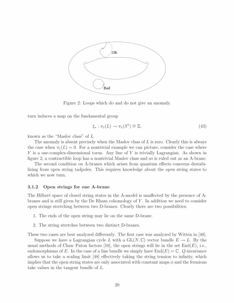
OK

Bad

Figure 2: Loops which do and do not give an anomaly.

turn induces a map on the fundamental group

ξ∗ : π1(L)→ π1(S1) ∼= Z, (43)

known as the “Maslov class” of L.The anomaly is absent precisely when the Maslov class of L is zero. Clearly this is always

the case when π1(L) = 0. For a nontrivial example we can picture, consider the case whereY is a one-complex-dimensional torus. Any line of Y is trivially Lagrangian. As shown infigure 2, a contractible loop has a nontrivial Maslov class and so is ruled out as an A-brane.

The second condition on A-branes which arises from quantum effects concerns destabi-lizing from open string tadpoles. This requires knowledge about the open string states towhich we now turn.

3.1.2 Open strings for one A-brane

The Hilbert space of closed string states in the A-model is unaffected by the presence of A-branes and is still given by the De Rham cohomology of Y . In addition we need to consideropen strings stretching between two D-branes. Clearly there are two possibilities:

1. The ends of the open string may lie on the same D-brane.

2. The string stretches between two distinct D-branes.

These two cases are best analyzed differently. The first case was analyzed by Witten in [48].Suppose we have a Lagrangian cycle L with a GL(N,C) vector bundle E → L. By the

usual methods of Chan–Paton factors [10], the open strings will lie in the set End(E), i.e.,endomorphisms of E. In the case of a line bundle we simply have End(E) = C. Q-invarianceallows us to take a scaling limit [48] effectively taking the string tension to infinity, whichimplies that the open string states are only associated with constant maps φ and the fermionstake values in the tangent bundle of L.

20

Thus, local operators corresponding to the insertion of open string states on the boundaryof Σ which maps to L are given by objects of the form

aI1I2...(φ)χI1χI2 . . . , (44)

where aI1I2...(φ) ∈ End(E), φ ∈ L, and χIk lies in the tangent bundle of L. The BRSToperator Q acts similarly to section 2.2 and so the Hilbert space of open string states isgiven by the total de Rham cohomology group

3⊕

n=0

Hn(L,End(E)), (45)

where the ghost number is given by n.The discussion of deformations of the theory induced by operators in section 2.2 applies

similarly to boundary states. One difference is that the deforming operator will naturallybe integrated along the one-dimensional ∂Σ rather than the two-dimensional Σ. Thus welook for ghost number one boundary operators to give the deformation. These correspondto elements of H1(L,End(E)).

It is interesting to explicitly match these deformations coming from open string vertexoperators to the parameters that define the A-model. First we note that the number ofdeformations of the connection on a flat vector bundle are given by H1(L,End(ER)) asshown in chapter 15 of [26] for example. Note that to count degrees of freedom correctlywe restrict to a real form of the gauge group. Since our open string operators are complex-valued, these deformations of the connection A account for exactly half of the degrees offreedom present in H1(L,End(E)).

So what do the other half of the deformations correspond to? Clearly deformations ofL itself should correspond to deformations of the A-model. We will now show that suchdeformations indeed account for the remaining degrees of freedom.

Let us assume initially the minimal case, i.e., that E is a line bundle. A deformationof L corresponds to a section of the normal bundle of L. We saw in section 3.1.2 that theKahler form provides a perfect pairing between vectors normal to L and vectors tangent toL. We may thus use the Kahler form to provide a one-to-one mapping between sectionsof the normal bundle of L and sections of the cotangent bundle of L. Thus a deformationis given by a 1-form on L. Of course, we would like the deformed submanifold to still beLagrangian. A simple calculation reveals that this condition dictates that the 1-form on Lbe closed.

The result is that Lagrangian deformations of L are in one-to-one correspondence withclosed 1-forms on L. In contrast, the degrees of freedom coming from the A-model consistof cohomology classes of 1-forms on L. Thus, if a deformation of L corresponds to a 1-form which is exact, then it does not affect the A-model. Such a deformation is called a“Hamiltonian” deformation of L. Thus we see that A-branes are really only defined up toHamiltonian deformation.

21

If the rank of E is greater than one then some of the deformations of L corresponding toH1(L,End(E)) are associated to breaking L up into a collection of branes with bundles oflower rank. This all ties together with the picture of enhanced gauge symmetry for coincidentD-branes as discussed in [50]. We should therefore think of the generic A-brane as comprisingof a line bundle E → L with higher rank bundles obtained by allowing such basic A-branesto coalesce.

There is one more piece of information about the properties of A-branes that the openstrings inH1(L,End(E)) can tell us. If an A-brane background defines a truly stable vacuumfor the topological A-model then the one-point function 〈Wa〉 will be zero for any vertexoperator associated with H1(L,End(E)). A nonzero value, called a “tadpole”, would forcethe operator to acquire an expectation value which would move the D-brane to anotherlocation.

We therefore need to know how to compute 〈Wa〉 exactly. Fortunately Witten [48] discov-ered a beautiful way of computing all the correlation functions between open string operatorsassociated to H1(L,End(E)).9

Without instanton corrections, Witten showed that the correlation functions could bedetermined by a Chern–Simons field theory on the Lagrangian L. The effect of instantonsis to add an additional term into the action. At tree level an instanton will consist of aholomorphic map of a disk into Y with the boundary of the disk mapped to L.

It is this instanton contribution to the effective action that has the potential to generatetadpoles 〈Wa〉. Restricting to the case of a line bundle, the condition that such tadpolesvanish is that

∑

α∈I

exp

(

2πi

∫

Dα

(B + iJ) + 2πi

∮

∂Dα

A

)

[∂Dα] = 0 in H1(L), (46)

where the sum is over all holomorphic disks Dα with ∂Dα ⊂ L (including multiple covers).The notation [∂Dα] refers to the cohomology class of ∂Dα. It is an interesting exercise toshow that (46) is invariant under Hamiltonian deformations of L.

Any Lagrangian violating (46) should not be considered to be an A-brane. This conditionon A-branes has been explored in some cases (in [51,52] for example) but a general geometricunderstanding appears to be missing. For example, it is not known if the 3-torus fibrationsof SYZ [53] satisfy this condition. Note that the condition (46) depends on B + iJ and thevalue of the connection A. Thus there can be A-branes which are good for a specific valueof these parameters but will, in general, be killed by tadpoles. Note also that an S3, whichis simply-connected, always trivially satisfies the vanishing tadpole condition.

It is worth summarizing the definition of an A-brane that we have finally settled on:

An A-brane is an element of the equivalence class of Lagrangian 3-manifolds inY modulo Hamiltonian deformations, which satisfies the tadpole cancellationproperty (46) and has trivial Maslov class.

9Note that Witten’s method applies to the topological field theory coupled to gravity.

22

Although we will be doing our best to evade the issue, we really should mention theA∞-algebra structure associated to the A-branes. The correlation functions for the openstring vertex operators which arise from Witten’s Chern–Simons theory are not consistentwith an associative algebra in the usual way. Instead one defines a series of products

mk(a1, a2, . . . , ak), (47)

for which m2 would be the usual product. These higher products are related in a specificway. We refer to [54–56], for example, for more details. The recent paper [57] explainscarefully how the A∞ structure appears directly in the topological field theory.

3.1.3 Open strings for many A-branes

Suppose we have a set of A-branes La. For simplicity of exposition, let us initially assumethat we just have line bundles over each brane. Given a pair of A-branes La and Lb we willhave a Hilbert space of open strings beginning on La and ending on Lb. This Hilbert spacehas a grading, which, up to an additive shift is the ghost number. This additive shift willturn out to be very important and we will discuss it extensively soon. We use the followingnotation for this graded Hilbert space:

Hom∗(La, Lb) =⊕

m∈Z

Homm(La, Lb). (48)

We will also denote Hom0(La, Lb) simply by Hom(La, Lb).The reason for this notation is that the concept of open strings between branes fits

naturally into the mathematical structure of a category. A category is defined as follows (ascopied from [58])

Definition 1 A category C consists of the following: a class10 obj(C) of objects, a setHomC(A,B) of morphisms for every ordered pair (A,B) of objects, an identity morphismidA ∈ HomC(A,A) for every object A, and a composition function

HomC(A,B)× HomC(B,C)→ HomC(A,C), (49)

for every ordered triple (A,B,C) of objects. If f ∈ HomC(A,B) and g ∈ HomC(B,C), thecomposition is denoted gf . The above data is subject to two axioms:

1. Associativity axiom: (hg)f = h(gf) for f ∈ HomC(A,B), g ∈ HomC(B,C) and h ∈HomC(C,D).

2. Unit axiom: idB f = f = f idA for f ∈ HomC(A,B).

There are many examples of a categories. Some of the obvious ones are as follows:

10A class is basically the same thing as a set but by using this language one avoids Russell’s paradox.

23

1. Objects are sets , morphisms are maps.

2. Objects are groups, morphisms are group homomorphisms.

3. Objects are rings (or modules, etc.), morphisms are ring homomorphisms (moduleshomomorphisms, etc.)

4. Objects are topological spaces, morphisms are continuous maps.

Note that in each case above an object is a set, or some glorified notion of a set, and soconsists of elements. One of the key ideas in category theory is to phrase things so that younever make any mention of these elements. There are also categories whose objects are notcomposed of elements. The D-brane categories which will be of particular interest to us areexamples of such “elementless” categories!

A morphism f ∈ Hom(A,B) is often written f : A → B for obvious reasons. As onemight guess, we say that two objects, A and B, in a category are isomorphic if there aremorphisms f : A → B and g : B → A such that gf = idA and fg = idB. That is, thereexists an invertible morphism between A and B.

L

L

L

1

2

3

Hom(L1, L2)⊗ Hom(L2, L3)→ Hom(L1, L3)

Figure 3: Composition of morphisms.

Clearly we would like to form a category where the A-branes are the objects and theopen strings of the A-model form the morphisms. While one is free to define the set ofmorphisms of the total Hilbert space as in (48), we will ultimately see that there is littledifference between this and restricting just to the case of Hom0(L1, L2).

The composition function corresponds precisely to the notion of two open strings joiningtogether as shown in open string diagram of figure 3. The edges of this figure have labelsshowing to which D-brane the ends of the open string are attached. This data is encoded inthe correlation functions of the topological field theory.

We see from the previous section that the identity operator idL for a given D-brane L isgiven by the identity operator in H0(L).

Just as in the case of a single D-brane, the correlation functions of the topological A-modelcoupled to gravity encode a more complicated product rule than the simple composition

24

(49). Thus the notion of an A∞-algebra is generalized to the notion of an A∞-category. Thisstructure is very interesting and important but we do not really need to concern ourselveswith it in these lectures. In particular, if one ignores the higher products, the category ofA-branes that we wish to construct really does satisfy the axioms of a plain old categoryspecified above.

The information content of the topological A-model with open strings is precisely thedata associated to the category of A-branes. We already know exactly what the objectsare. We now want to compute the dimensions of the Hilbert spaces of open strings and thecorrelation functions between such states.

To compute the Hilbert space of open strings stretched between two different D-branesL1 and L2, it is easiest to assume that L1 and L2 intersect transversely. As in section 3.1.2,the Q-invariance of the topological field theory can be used to argue that open strings canonly arise from constant maps φ : Σ→ Y . This means that an open string state is associatedto a point of intersection L1 and L2.

The previous section suggests that locally the Hilbert space should be given by the DeRham cohomology of this intersection, i.e., the cohomology of a point. We therefore firstguess that there is a one-dimensional Hilbert space associated with each point of intersection.Thus the dimension of Hom∗(L1, L2) would be given by the number of points of intersectionbetween L1 and L2.

This cannot be right. We know the A-model is invariant under Hamiltonian deformationof L1 or L2 but the number of points of intersection is not such an invariant. Of course, theoriented intersection number #(L1∩L2) is such an invariant as it depends only on homologyclasses but this turns out to be too crude for our purposes.

Let us introduce some notation. Let there be M points of intersection between L1 andL2 and let the points be labeled pa, a = 1 . . .M . Thus we have open string vertex operatorsWpa

that create an open string at the point pa. Our putative Hilbert space will be denotedV = CM . Each vertex operator Wpa

has a ghost number that we denote µ(pa). This leadsto a grading of V by ghost number

Vi =⊕

µ(pa)=i

C

V =⊕

i

Vi.(50)

The way to determine the true Hilbert space lies in Witten’s work on Morse theory [59]as generalized in the work of Floer [60] and, in particular, by Fukaya [61, 62]. We also referto chapters 10.5 and 40.4 of [8] for a nice review of this. Because these references are quitethorough, we will only outline the general picture in the following discussion.

The basic idea is that an instanton can “tunnel” from an open string state at one pointof intersection to an open string at another point of intersection. The worldsheet of aninstanton of such a tunneling process is shown in figure 4. As we saw earlier, at tree-level these worldsheet instantons are holomorphic disks in Y . These instantons produce a

25

L L1 2

Worldsheet

Perturbative Ground States

Figure 4: Instanton Tunneling.

correction to the BRST operator resulting in:

Q,Wpa =

∑

b

nabWpb, (51)

for some coefficients nab to be determined. Thus the true Hilbert space will be determined asthe Q-cohomology of some complex based on the vector space V . Since Q has ghost numberone, the complex looks like

. . .Q

V−1Q

V0Q

V1Q

. . . (52)

We define Homi(La, Lb) as the cohomology of this complex at position i.To compute nab we must perform an integral of the moduli space of instantons. This

integral must be performed over the fermionic parameters as well as the obvious bosonicmaps φ. By the usual rules of fermionic integration such an integral vanishes unless thefermionic parameters cancel in some way, i.e., we have no net fermionic zero modes. To bemore precise, we require that the index of the Dirac operator for the instanton is equal tothe ghost number of Q, i.e., one [59].

The index of the Dirac operator also measures the generic (or, to be precise, virtual)dimension of the moduli space of holomorphic maps. We refer to [63] for a nice account ofwhat happens in the non-generic situation. In the generic case, we thus compute nab simplyby counting the number of points in the zero-dimensional instanton moduli space.

For an instanton connecting pa to pb, the index of the Dirac operator is given by thedifference in ghost numbers µ(pb)−µ(pa). Thus we expect that the generic dimension of themoduli space of instantons is given by

dim M = µ(pb)− µ(pa)− 1. (53)

We refer the reader to [64] for further information on this point.The astute reader should have noticed that we have nowhere specified a way that one can

actually compute µ(pa). Given the dimensions of moduli spaces of instantons, the relation

26

L

L

L2

1

3

Figure 5: Disk instanton associated to three-point functions.

(53) only gives enough information to compute the relative ghost number of two points ofintersection of La and Lb. Indeed, we have the following very important fact:

The topological A-model does not contain enough information to determine theabsolute ghost number of an open string associated to a point of intersectionof two A-branes.

Just how much ambiguity in the ghost number do we actually have? Given a pair of D-branes L1 and L2 we are free to shift the ghost numbers of the open strings from L1 to L2 bysome fixed integer. We also saw in section 3.1.2 that if L1 = L2 then the ghost number wasgiven by the degree of de Rham cohomology which is perfectly well-defined. Furthermore,we would like to preserve ghost number in the operator product

Homi(L1, L2)⊗ Homj(L2, L3)→ Homi+j(L1, L3). (54)

The ambiguity in the ghost number can then be accounted for by assigning a ghost numberµ(L) to each D-brane itself. One then defines the ghost number of an element of Homi(La, Lb)as

i+ µ(Lb)− µ(La). (55)

It is easy to see that this definition has all the properties we desire.We may restate the above as follows. The topological A-model has a symmetry which

allows us to shift the ghost numbers of the open string states by assigning arbitrary ghostnumbers to the A-branes and defining the ghost number as in (55). Note that this idea ofassigning integers to Lagrangian submanifolds to fix this ambiguity was studied carefullyin [65].

We will not give details on how to compute the correlation functions. It should be clearhowever that there will be instanton corrections involved. For example, if we compute thethree-point function associated to figure 3, at tree-level we will consider holomorphic disksin Y with boundary conditions shown in figure 5. The cancellation of fermion zero modeswill enforce ghost number conservation as usual.

27

In this section we have outlined the definition of the category of A-branes in the casethat the objects La and Lb intersect transversely. Actually one may always use Hamiltoniandeformations to deform any pair of Lagrangian into this case. Thus we actually have acomplete definition of the category of A-branes.

This category is named after Fukaya who introduced it. The reader should note thatour discussion of the Fukaya category in this section has omitted a vast number of technicaldetails that have made this subject the object of a good deal of attention for the pastten years. We refer to [56, 62, 66–68], for example, for more of the gory details. We alsorefer to [69, 70] where the Fukaya category (complete with its A∞ structure) is determinedexplicitly for the 2-torus. Recently, in a remarkable paper [71], Seidel has described theFukaya category for the quartic K3 surface. No other examples are known.

The generalization of the Fukaya category to the case of higher rank bundles over eachA-brane should be fairly obvious. Rather than associating C with each point of intersection,we have a matrix representing a linear map from the fibre of one bundle to the fibre of theother over the point of intersection.

We emphasize that nothing in A-model depends on the complex structure of Y . Indeed,the Fukaya category is usually defined purely in terms of the symplectic geometry of Ythus explicitly removing any possible dependence on the complex structure. The Fukayacategory depends on B + iJ for both its objects and its composition of morphisms. Thetadpole condition (46) has a B + iJ dependence and so certain objects might only exist forparticular values of this parameter. The correlation functions depend on B + iJ throughinstanton corrections and so the composition of morphisms are similarly dependent.

Finally we should point out that worldsheet instantons are generally expected to adverselyaffect notions based on the concept of a spacetime metric. Thus it would be reasonable toexpect that the concept of a Lagrangian submanifold is only really valid at large radiuslimit. The composition rules in the Fukaya category are based on power series associated toinstanton effects. Beyond the radius of convergence of these power series it is reasonable tothink that the Lagrangian submanifold description of A-branes has broken down.

3.2 The B-model

It should be with relief that we turn attention to the B-model on X. Unfortunately we willsee that there is a subtlety concerning the set of all possible B-branes that will occupy usfor most of the remaining lectures.

3.2.1 B-branes

We may repeat the analysis of the beginning of section 3.1.1. The difference for the caseof B-branes is that the B-model twist implies that we should impose Rı

j = Ri = 0 for the

reflection matrix in (38) and (39). That is, only the diagonal terms Rij and Rı

are nonzero.This means that the almost complex structure now preserves the tangent and normal

directions to the D-brane, rather than exchanging them. It follows that the D-brane is

28

a holomorphically embedded submanifold of X. Clearly this forces the dimension of theD-brane to be even, i.e., 0, 2, 4 or 6.

Although 0, 2 and 4-dimensional B-branes exist, we will at first restrict attention onlyto the 6-dimensional case, where the D-brane fills X. That is we put purely Neumannconditions on the open string. The complexities of B-branes will allow us to deduce theproperties of all the B-branes purely from a knowledge of 6-branes.11

As in the A-brane, consideration of the B-field forces us to consider the possibility of abundle over the B-brane, i.e., a bundle E → X. Setting the B-field equal to zero we mayconsider the constraint on this bundle from the requirement that the variation of the actionfrom the boundary term is zero. In this case, we find that the curvature, F , of the bundle isa 2-form purely of type (1,1) [8, 43, 48]. In other words, E → X, is a holomorphic bundle.

We refer again to chapter 15 of [26] for a very readable account of holomorphic vectorbundles. The basic idea is that the transition functions for the bundle may be written asholomorphic functions of the coordinates of X. Thus the bundles may be described verynaturally in the language of algebraic geometry. In section 4 this will allow us to move fromthe language of bundles to the language of sheaves which, although alien to most physicists,is definitely the right language for B-branes.

3.2.2 Open strings for B-branes

Since we have chosen purely Neumann boundary conditions on the open string, we haveeffectively set the matrix R equal to the identity in (39). Thus, from (24) we have, on theboundary

θj = gjk(ψk+ − ψk

−) = 0, (56)

and so a local operator will depend only on φ and η. It follows that local operators looklike (0, q)-forms.

Suppose we have two B-branes in the form of two bundles E1 → X and E2 → X. TheChan–Paton degrees of freedom are associated with maps from E1 to E2. We denote thespace of such maps as Hom(E1, E2).

We saw in section 2.3 that the BRST operator Q looks like the Dolbeault operator in theB-model. Adding all these ingredients together, we see that an open string vertex operatorfor a string stretching from E1 to E2 is given by the cohomology groups

H0,q

∂(X,Hom(E1, E2)). (57)

In contrast to the A-brane case, we can choose to declare the ghost number of an operatorin (57) to be q without ambiguity.

11Note that, in our notation, a p-brane is a brane with p-dimensions in the Calabi–Yau directions and anynumber of dimensions in the uncompactified part of spacetime.

29

As always, the B-model has no instanton corrections. If

a ∈ H0,1

∂(X,Hom(E1, E2))

b ∈ H0,1

∂(X,Hom(E2, E3))

c ∈ H0,1

∂(X,Hom(E3, E1)),

(58)

then we may compute the 3-point function exactly from

〈WaWbWc〉 =

∫

X

Tr(a ∧ b ∧ c) ∧ Ω, (59)

and deduce an operator product algebra. The Hom matrices are composed in the obviousway.

If the B-model is coupled to gravity one may analyze higher n-point functions. In [48]Witten showed that these correlation functions could be deduced from a “holomorphic”Chern–Simons theory. This A∞ structure was analyzed more abstractly by Merkulov [72].See also [57] for more discussion of the A∞ structure in topological field theories.

3.2.3 A failure of mirror symmetry

Given the dreadful complexities one is forced to endure to define the Fukaya category (mostof which we omitted) the reader is probably shocked at how easy the B-branes were toanalyze.

It would be remarkable if one could now invoke mirror symmetry and say that the categoryof A-branes on Y is equivalent to the category of B-branes on X at this point. Unfortunatelythis equivalence would be wrong with our current definition of B-branes. The problem isthat we simply do not have enough B-branes.

Clearly our assumption that B-branes are 6-branes is too strong. The lower-dimensionalbranes certainly exist and one might hope that such branes account for the missing B-branes.Sadly we still fall far short of the number of objects in the Fukaya category.

There is a lack of symmetry between the A-branes and B-branes which is key in thefailure of mirror symmetry. In section 3.1.3 we had a real problem when we tried to assignan intrinsic ghost number to an open string which we solved by labeling the A-branes witha ghost number. The B-branes did not have this problem. We will essentially restore mirrorsymmetry by inflicting the ghost number ambiguity on the B-branes!

As Kontsevich proposed as far back as 1994 [73], the answer involves going to the “derivedcategory” as we will explain in section 5.

4 Some Mathematical Tools

Before continuing with the story of B-branes we need some more mathematical weapons. Asthese ideas are not familiar to a typical physicist we will try to be fairly thorough. Most ofthe ideas in this section are taken from [58,74, 75].

30

As defined in section 3.2, a B-brane is associated to a vector bundle over X. In section 2.3we noted that the B-model for a closed string can be described in purely algebraic terms. Inorder to do the same for closed strings we need to replace vector bundles by something purelyalgebraic, namely sheaves. This mathematical construction appears to be unavoidable if onewants to fully understand B-branes. Anyone who ignores the language of sheaves would beforced to reinvent it!

In order to discuss sheaves properly we use quite a bit of categorical language. This willalso prove useful later on when we discuss the derived category.

4.1 Categories of sheaves

4.1.1 Holomorphic functions

Let us begin with PN with homogeneous coordinates [z0, z1, . . . , zN ]. Let X ⊂ PN be an“algebraic variety”, i.e., X is defined as the intersection of the zeroes of a set of polynomialsF1, F2, . . . in the homogeneous coordinates. These polynomials define the space X purely interms of algebraic data. Other than PN itself, the simplest case consists of a hypersurfaceX ⊂ PN defined by a single equation. We never consider more than one defining equationin these lectures.

How might we put some more “stuff” on X that is described purely in terms of algebraicstructures built on the homogeneous coordinates? The obvious thing to do is to definefunctions f : X → C. In terms of the homogeneous coordinates, the natural way to definesuch a function is

f =g

h, (60)

where g and h are polynomials in the homogeneous coordinates. Clearly we require g and hto have the same homogeneous degree so that the function is well-defined on the projectivespace PN and thus X. Any function f : X → C that can be written in the form (60) in aneighbourhood of a point p ∈ X, such that h never vanishes in this neighbourhood, is calledregular at p. A function is regular on X if it is regular at all the points in X. We will alsorefer to such functions on X as holomorphic. It is these regular functions on X which formthe prototype of “extra data” on X which will be used to replace the unalgebraic notion ofa vector bundle.

4.1.2 Sheaves

Let X be a topological space. We make the following12

Definition 2 A presheaf F on X consists of the following data

a) For every open set U ⊂ X we associate an abelian group F (U).

12In fancy language this makes a presheaf a contravariant functor from the category of open sets on X tothe category of abelian groups.

31

b) If V ⊂ U are open sets we have a “restriction” homomorphism ρUV : F (U)→ F (V ).

This data is subject to the conditions

0. F (∅) = 0.

1. ρUU is the identity map.

2. If W ⊂ V ⊂ U then ρUW = ρV WρUV .

If σ ∈ F (U) then we use the notation σ|V for the restriction ρUV (σ). An element of F (U)is called a section of F over U . X is an open subset of itself and an element of F (X) iscalled a global section.

We then make a more restrictive

Definition 3 A sheaf F on X is a presheaf satisfying the conditions

3. If U, V ⊂ X and σ ∈ F (U), τ ∈ F (V ) such that σU∩V = τU∩V , then there existsν ∈ F (U ∪ V ) such that ν|U = σ and ν|V = τ .

4. If σ ∈ F (U ∪ V ) and σU = σV = 0, then σ = 0.

This definition makes the data defining a sheaf essentially contained in very small open sets.That is, the sheaf is defined by “local” information.

A simple example of a presheaf is given by associating some fixed abelian group, suchas Z, to every non-empty open set in X. The restriction maps are set equal to the identity.This example is not a sheaf as it violates condition 3 above when we consider disconnectedopen sets. The closest sheaf we can find to this presheaf would be to associate Zn to eachopen set U where n is the number of connected components of U . This latter sheaf will beuseful and we denote it simply by Z.

Another important sheaf is constructed by making F (U) the group (under addition) ofholomorphic functions over U . The restriction map is the obvious restriction map in theusual sense. This “sheaf of holomorphic functions”, also known as the structure sheaf, isdenoted OX (or just O).

Yet another example is given by O∗ — the sheaf of nonzero13 holomorphic functions.This time the abelian group structure is given by multiplication.

It will be useful to make a category of sheaves. Obviously the sheaves on X form theobjects. We define a morphism φ : F → G of sheaves as something which associates ahomomorphism φ(U) : F (U) → G (U) to each open set U ⊂ X such that, for any V ⊂ U ,the following diagram commutes:

F (U)φ(U)

ρUV

G (U)

ρ′UV

F (V )φ(V )

G (V ),

(61)

13That is, nowhere zero.

32

where ρ and ρ′ are the restriction maps on F and G respectively. The fact that this formsa category follows immediately from the properties of homomorphisms of groups. Note thatthe objects, F , in the category of sheaves are not directly composed of elements. Havingsaid that, for any open set, F (U) is a group and so is composed of elements.

We note that two sheaves are said to be isomorphic if there is an invertible morphismfrom one to the other.

4.1.3 Locally free sheaves

Having defined the structure sheaf OX, we would like to define more complicated sheavesthat are equally algebraic in nature. First recall the definition of a module:

Definition 4 Let R be a ring with a multiplicative identity 1. An R-module is an abeliangroup M with an R-action given by a mapping R×M → M such that

1. r(x+ y) = rx+ ry

2. (r + s)x = rx+ sx

3. (rs)x = r(sx)

4. 1x = x

for any r, s ∈ R and x, y ∈M .

Now, the set of regular functions over U , OX(U), is an abelian group under addition asnoted earlier, but multiplication of functions also gives it a ring structure. This allows us tointroduce the concept of a sheaf of OX-modules. That is, let E be a sheaf such that E (U) isan OX(U)-module for any open U ∈ X. By a common abuse of notation we will refer to asheaf of OX-modules as an OX-module.

Clearly OX is itself an OX-module. We may also take a sum of copies

O⊕nX = OX ⊕ OX ⊕ . . .⊕OX

︸ ︷︷ ︸

n

(62)

to give another OX-module. This is called the free OX-module of rank n. We call a sheaf E

locally free of rank n if there is an open covering Uα of X such that E (Uα) ∼= OX(Uα)⊕n

for all α.There is a one-to-one correspondence between holomorphic vector bundles of rank n on

X and locally free sheaves of rank n on X. To see this first consider the trivial complex linebundle over X. We may regard OX(U) as the group of holomorphic sections of this bundleover U . Thus, if the covering Uα trivializes a vector bundle E → X, then the group ofholomorphic sections of E over Uα is given by OX(Uα)⊕n.

Conversely, let E be a locally free sheaf and let

φα : E (Uα)→ OX(Uα)⊕n, (63)

33

be the explicit isomorphism. On Uα ∩ Uβ we may define the n × n matrix of holomorphicfunctions

φβφ−1α : OX(Uα ∩ Uβ)⊕n → OX(Uα ∩ Uβ)⊕n, (64)

which defines a holomorphic bundle E → X.So locally free sheaves are the algebraic way of describing holomorphic vector bundles.

Clearly a trivial bundle corresponds to a free OX-module and, as we stated above, the trivialline bundle corresponds to the structure sheaf OX .

To get a better feel for locally free sheaves, let us consider some very simple cases whereX is P1 with homogeneous coordinates [z0, z1]. We define an open set U0 by z0 6= 0 with anaffine coordinate y0 = z1/z0. Similarly U1 has z1 6= 0 with an affine coordinate y1 = z0/z1.Thus P1 has an open cover U0, U1.

Consider a holomorphic line bundle on P1 with a fibre coordinate wi over the open setUi. Then the transition function in U0 ∩ U1 may be written in the form

w1 = yn1w0, (65)

for some integer n.14 We define O(n) as the locally free sheaf associated to this line bundle.Clearly O(0) is O .

Now consider an example of a morphism O → O(n). On U0 we use the identity map 1.To keep the transition function valid, this would force us to make the morphism look likeg(y1) 7→ yn

1 g(y1) on U1 for any g ∈ O(U1). We will write a morphism as

Of

O(n), (66)

where f is a homogeneous function in [z0, z1] and we understand the morphism in Uα to begiven by a multiplication by f/zn

α. Thus, in the case we just described, f = zn0 . Clearly, so

long as f is homogeneous of degree n, it will be compatible with the transition functions ofthe vector bundle. Indeed, all morphisms from O to O(n) are of this form.

Grothendieck [76] proved that any locally free sheaf of finite rank on P1 is isomorphicto a sum O(n1) ⊕ O(n2) ⊕ . . .. For PN we may define analogous sheaves O(n) which willserve as our basic building blocks later on. Note that Grothendieck’s theorem is not validfor N > 1.

4.1.4 Kernels and cokernels

Given a morphism between two objects in a category we would like to define the notion ofkernel and cokernel of this map.

If we have a map f : B → C between two groups we would usually define the kernelof f , Ker(f), to be the subgroup of B which f maps to the identity of C. In the world ofcategories it is taboo to talk about elements and so this definition is, in general, no good.

The first thing we need to define is the notion of the identity in some categorical way.This is done as follows

14This is the first Chern class of the line bundle.

34

Definition 5 A zero object in a category is an object 0 such that for any object B thereis precisely one morphism in Hom(0, B) and precisely one morphism in Hom(B, 0). If thezero object exists, then for any pair of objects, B and C, we define the zero morphism (alsodenoted as 0) in Hom(B,C) as the composition B → 0→ C.

It is easy to show that all zero objects are isomorphic. For the category of sets the zero objectdoes not exist. For groups, rings, etc., it is the trivial group, ring, etc. In the category ofsheaves it is the sheaf that associates the trivial group to every set U . In the category ofD-branes, it represents the absence of a D-brane!

Secondly, we are going to restrict attention to additive categories. This is a category witha zero object and an abelian group structure (written as addition) on the set of morphismsHom(B,C) such that the distributive law (f + f ′)g = fg + f ′g and f(g + g′) = fg + fg′

is true for compositions.15 It is easy to see that the zero morphism is the identity in thegroup Hom(B,C). Clearly the category of abelian groups and the category of sheaves hasan additive structure. In addition, we saw that for D-branes Hom(B,C) represents a Hilbertspace, thus endowing the category of D-branes with an additive structure too.

Now we may make the following

Definition 6 The kernel of a morphism f : B → C is a morphism i : A → B such thatfi = 0 and which satisfies the following “universal” property: For any morphism e : A′ → Bsuch that fe = 0, there is a unique morphism e′ : A′ → A such that e = ie′. That is, themap e′ can be constructed such that the following commutes:16

A′

e′e

Ai

Bf

C.

(67)

Note that the kernel may not always exist for a general additive category. We emphasizethat, in this categorical language, a kernel is a morphism — not an object as one mightfirst think. Of course, since a morphism must specify the object it is mapping from, wedo intrinsically define a kernel object , A, too. If the reader is unfamiliar with universalproperties of maps such as the above, they should convince themselves that this definitionof kernel coincides with the usual one for, say, the category of groups. To be precise, thekernel, as defined above, is the inclusion map of the kernel subgroup into the group itself.

We say f is a monomorphism if the kernel of f is zero. It is easy to prove that the unique-ness of e′ implies that the kernel itself is a monomorphism. For groups, etc., a monomorphismis the same thing as an injective map. If the kernel object exists, it is unique up to isomor-phism.

While we’re at it, we can reverse all the arrows in the above to define the cokernel:

15In addition one requires the existence of an object B ⊕ C for every pair B and C, but this isn’t veryimportant in this discussion.

16In these diagrams the solid lines represent maps which are given, and dotted lines represent maps to beconstructed.

35

Definition 7 The cokernel of a morphism f : B → C is a morphism p : C → D such thatpf = 0 and which satisfies the following “universal” property: For any morphism g : C → D′

such that gf = 0, there is a unique morphism g′ : D → D′ such that g = g′p. That is, themap g′ can be constructed such that the following commutes:

Bf

Cp

g

D

g′

D′

(68)

The object D is called the cokernel object. Recall that the “old” definition of the cokernel ofa map f : B → C is the quotient C/ Im(f). The reader should again check that this agreeswith the categorical definition.

We say f is an epimorphism if the cokernel of f is zero. For groups, etc., an epimorphismis the same thing as a surjective map. Again, the cokernel itself is an epimorphism and thecokernel object is unique, if it exists, up to isomorphism.

So why have we dragged ourselves through all this mathematical nonsense? The answer isthat the category of sheaves does not quite behave as one might expect when this categoricalmachinery is applied to it. One might be forgiven for thinking that given a map betweensheaves, φ : F → G , one could apply the old ideas of kernel and cokernel to the group mapsφ(U) : F (U) → G (U) to get a definition of kernel and cokernel of φ. While this works forthe kernel, it can fail for the cokernel. In particular, the cokernel defined this way, whilealways a presheaf, need not be a sheaf.

To illustrate what can go wrong, consider the morphism of sheaves

φ : O → O∗, (69)

on C∗ = C − 0 by the map φ(U)(f) = exp(2πif) for any function f ∈ O(U). Thecoordinate z on the complex plane gives us a global section z ∈ O∗(C∗). This section isclearly not in the image of φ(C∗). However, if we were to consider a simply-connectedsubspace U ∈ C∗, then z|U would lie in the image of φ(U). We can define a nontrivialpresheaf F such that F (U) is given by O∗(U)/ Im(φ(U)), but it violates property number4 of the definition of a sheaf in section 4.1.3.

Conversely, the categorical definition of cokernel tells us that cokernel of φ in this exampleis zero. Thus φ is an epimorphism.

4.1.5 Abelian categories

A particular kind of category will be of particular importance to us — namely an abeliancategory. While the D-brane category itself will turn out not to be abelian, these specialcategories will be an essential building block in describing D-branes.

We defined the kernel and cokernel morphisms in section 4.1.4. Now let us further definethe image of a map as the kernel of its cokernel (if it exists) and the coimage of a map as

36

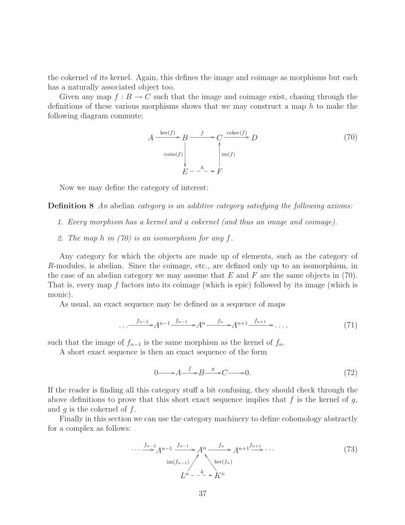
the cokernel of its kernel. Again, this defines the image and coimage as morphisms but eachhas a naturally associated object too.

Given any map f : B → C such that the image and coimage exist, chasing through thedefinitions of these various morphisms shows that we may construct a map h to make thefollowing diagram commute:

Aker(f)

Bf

coim(f)

Ccoker(f)

D

Eh

F

im(f)

(70)

Now we may define the category of interest:

Definition 8 An abelian category is an additive category satisfying the following axioms:

1. Every morphism has a kernel and a cokernel (and thus an image and coimage).

2. The map h in (70) is an isomorphism for any f .

Any category for which the objects are made up of elements, such as the category ofR-modules, is abelian. Since the coimage, etc., are defined only up to an isomorphism, inthe case of an abelian category we may assume that E and F are the same objects in (70).That is, every map f factors into its coimage (which is epic) followed by its image (which ismonic).

As usual, an exact sequence may be defined as a sequence of maps

. . .fn−2

An−1 fn−1

An fnAn+1 fn+1

. . . , (71)

such that the image of fn−1 is the same morphism as the kernel of fn.A short exact sequence is then an exact sequence of the form

0 Af

Bg

C 0. (72)

If the reader is finding all this category stuff a bit confusing, they should check through theabove definitions to prove that this short exact sequence implies that f is the kernel of g,and g is the cokernel of f .

Finally in this section we can use the category machinery to define cohomology abstractlyfor a complex as follows:

. . . fn−2

An−1fn−1

Anfn

An+1fn+1 . . .

Ln

im(fn−1)

kKn

ker(fn)

(73)

37

If fnfn−1 = 0, the definition of the kernel of fn guarantees the existence of the map k above.The cohomology of this complex at position n is then defined as the cokernel object of themap k. We generally denote the cohomology Hn(A•) in the case that it is an abelian group,or H n(A•) if it is a sheaf.

There is a remarkable theorem due to Freyd [77] that says that, if the objects in anabelian category can be described as a set, the category may be embedded in the categoryof R-modules for some ring R. This effectively means that the objects in such a categorycan be thought of as consisting of elements.

We will see eventually that the categories we build for A-branes and B-branes are notabelian — hence the necessity for the abstractions of category theory.

4.1.6 Coherent sheaves

We saw in section 4.1.3 that the concept of vector bundles can be replaced by locally freesheaves in algebraic geometry. We want to be able to do things like compute cohomologyfor complexes of these things so it would be nice if the category of locally free sheaves werean abelian category. Sadly it is not.

The problem is that, while this category contains all of its kernels, it does not containits cokernels. The solution is to start with the category of locally free sheaves, which is asubcategory of the category of OX-modules. Then add in all the cokernel objects togetherwith all the possible morphisms between these new objects and the objects we already had.The resulting category is abelian. Thus we end up with a minimal abelian full17 subcategoryof the category of OX-modules containing locally free sheaves. This is the category of coherentsheaves.18

Let’s give a simple example of a coherent sheaf that is not locally free. We work locallyon part of X and pretend it looks like C3 with affine coordinates (x, y, z). Consider thefollowing morphism

O⊕3 ( x y z )O , (74)

that is, three functions f1, f2, and f3 are mapped to xf1+yf2+zf3 by this morphism. Naıvelyspeaking, the cokernel object should consist of functions on C modded out by functions inthe image of the map. This quotient should kill all functions away from the origin. Wedefine Op as the sheaf such that Op(U) is the trivial group if U does not contain the origin.If U does contain the origin we set Op(U) = C. This is an OX-module and is called theskyscraper sheaf of the origin. There is also a natural map

O Op, (75)

17A subcategory is full if, for any pair of objects A and B, the set of morphisms Hom(A, B) is the samein the subcategory as it was in the original category.

18In these notes we are going to be somewhat careless about specifying whether ranks of free modules areinfinite or finite. In particular we will make no effort to distinguish between coherent and quasi-coherent

sheaves.

38

which takes a function to its value at the origin. The reader can carefully check through thedefinitions to see that (75) indeed represents the cokernel of (74). That is,

O⊕3( x y z )O Op 0 (76)

is an exact sequence.Thus, the skyscraper sheaf Op is a coherent sheaf. It clearly isn’t locally free since its

rank appears to jump at the origin. In a way, it looks like it could be associated to a vectorbundle which has a fibre C over the origin and has trivial fibre elsewhere. We will see insection 5.4 that this is a 0-brane on X.

We can also compute the image of the map (74), i.e., the kernel of the map (75). Tophrase it a third way, we are looking for the OX-module Ip that completes the short exactsequence

0 Ip O Op 0. (77)

One can easily show that Ip is a subsheaf of O and consists of functions which vanish atthe origin. This sheaf is called the ideal sheaf of the origin.

Again, Ip is not locally free. The best we could say is that somehow it represents atrivial bundle with fibre C3 everywhere except at the origin, where it has no fibre. In D-brane language you might say it is a 6-brane on X with an anti-0-brane glued in at theorigin. We will see later that this isn’t such a bad description of Ip.

4.2 Cohomology

We have replaced the vector bundles of the B-model by coherent sheaves. We now need toreplace the notion of Dolbeault cohomology with something more algebraic. To do this weuse sheaf cohomology. Let us emphasize immediately that by sheaf cohomology we do notmean Cech cohomology, which is more topological than algebraic.19 Our sheaf cohomologyis the version due to Grothendieck as reviewed in chapter III of [74] which is much moresuited to the B-model. Having said that, we will start our discussion with Cech cohomology.

4.2.1 Cech cohomology

Here we give a lightning review. For more information and examples, the reader is referredto [79].

Suppose U = Uα is an open covering of a manifold X. Let us denote Uα0∩Uα1

∩. . .∩Uαp

by Uα0α1...αp. Given a sheaf F we define

Cp(U,F ) =∏

α0<α1<...<αp

F (Uα0α1...αp). (78)

That is, an element a ∈ Cp(U,F ) is specified by giving an element aα0α1...αp∈ F (Uα0α1...αp

)for each unordered (p+ 1)-tuple of open sets in U.

19Unfortunately, many references, such as [78], do mean Cech cohomology when they say sheaf cohomology.

39

Now define a coboundary δ : Cp → Cp+1 by

(δa)α0α1...αpαp+1=

p+1∑

k=0

(−1)kaα0α1...αk ...αp+1, (79)

where the notation αk means omit αk.It is easy to prove that δ2 = 0 and so we can define Cech cohomology, Hp(U,F ), as the

cohomology of the complex

0 C0(U,F )δC1(U,F )

δC2(U,F )

δ. . . (80)

This definition of Cech cohomology depends on the open covering U but one can show that,as the covering becomes finer and finer, one approaches a well-defined limit which we callHp(X,F ). An open cover which yields Hp(U,F ) ∼= Hp(X,F ) is a so-called good coverwhere each finite intersection Uα0

∩ Uα1∩ . . . ∩ Uαp

is diffeomorphic to Rn. We refer to [79]for more details.

As is well-known, given a short exact sequence of sheaves

0 E F G 0, (81)

we have an associated long exact sequence of cohomology:

. . . Hk(X, E ) Hk(X,F ) Hk(X,G ) Hk+1(X, E ) . . . (82)

Also, if X is an n-dimensional manifold, then Hk(X,F ) = 0 for any F if k < 0 or k > n.It will prove useful to know all the cohomology groups Hk(Pn,O(m)) for the locally-

free sheaves of rank one introduced in section 4.1.3. The zeroth Cech cohomology consistsof sections defined over each Uα such that the differences of these sections over the pair-wise intersections vanishes. In other words, the zeroth Cech cohomology consists of globalsections.

The global sections of a sheaf F which is an OX-module are in one-to-one correspondencewith morphisms OX → F . This important fact will be used many times below. Themorphism may be produced from the section simply by multiplication by the section. Giventhe morphism, the definition of morphisms between OX-modules forces it to be given bymultiplication by a global section.

The analysis around (66) therefore shows that global sections of O(m) are given byhomogeneous functions of degree m in the homogeneous coordinates [z0, z1, . . . , zn]. Thus,

dim H0(Pn,O(m)) =

(n+m

m

)

, (83)

where the binomial coefficient is defined to be zero if either of its entries are negative.

40

The method of Cech cohomology may be applied to compute the higher cohomologies.This is tedious and there are other ways to do the computation (see [74, 78] for example).The result is that

dim Hk(Pn,O(m)) = 0 for k 6= 0, n

dim Hn(Pn,O(m)) =

( −m− 1

−n−m− 1

)

.(84)

Now suppose X ⊂ Pn is an algebraic variety of dimension n − 1 corresponding to thezeroes of a polynomial f of homogeneous degree d. We denote the embedding i : X → Pn.

Let us introduce a little notation. Suppose we have a map f : X → Y between twoalgebraic varieties and a sheaf F on X. We may define the sheaf f∗F on Y by f∗F (U) =F (f−1U). More specifically, suppose we have an embedding i : X → Pn, and we are given asheaf E on X. The sheaf i∗E is therefore given by i∗E (U) = E (U ∩ Pn) for all open subsetsU ⊂ Pn. This naturally embeds the set of sheaves on X into the sheaves on Pn.

The structure sheaf OX may thus be pushed forward into a sheaf i∗OX on P4. By amodest abuse of notation we refer to this latter sheaf as OX . Clearly OX is then a quotientsheaf of O . In fact, it is not hard to see that we have a short exact sequence of sheaves

0 O(−d) fO OX 0. (85)

Using (82), and the fact that Hk(X,F ) = Hk(Pn, i∗F ), this allows the computation of thecohomology of OX . Similarly we may tensor (85) by O(m) to compute the cohomology ofOX(m) = OX ⊗ O(m).

4.2.2 Spectral sequences

We would like to compare Cech cohomology with something we already know about such asDolbeault cohomology. A very quick way of doing this is to use “spectral sequences” whichwe now review. The idea of spectral sequences will also be a recurring topic in the rest oflectures. Again, a comprehensive review of this important subject is beyond the scope ofthese lectures and we recommend the interested reader consult [79,80], for more information.Here we focus on how a spectral sequence is used rather than why it works.

41

Suppose we are given a double complex, Ep,q0 ,

......

...

E0,20

δ

d

E1,20

δ

d

E2,20

δ

d

. . .

E0,10

δ

d

E1,10

δ

d

E2,10

δ

d

. . .

E0,00

δ

d

E1,00

δ

d

E2,00

δ

d

. . .

p

q

(86)

where each row and each column forms a complex. We assume that the two derivativesanticommute dδ + δd = 0.

Clearly we may make a new complex

0 E0 DE1 D

E2 D . . . , (87)

whereEn =

⊕

p+q=n

Ep,q0 , (88)

and D = d+ δ. The big question is, how to we compute the cohomology of (87)?The spectral sequence method is to inductively form a sequence of stages Ep,q

r . Ep,qr+1 is

defined as the cohomology of Ep,qr with respect to a differential

dr : Ep,qr → Ep+r,q−r+1

r , (89)

where d0 is given by d in figure (86) and d1 is given by the image of δ in Ep,q1 . We won’t

need to know how to compute dr for r ≥ 2 since any problem that requires such knowledgeis essentially too difficult for these lectures!

For large enough r (r ≥ 2 if we’re lucky) the differentials dr are all zero. This means that,for large r, the Ep,q

r ’s become independent of r and so are written Ep,q∞ . The cohomology of

(87) is then given as20

HnD =

⊕

p+q=n

Ep,q∞ . (90)

4.2.3 Dolbeault cohomology

Let’s try the spectral sequence construction to prove that Dolbeault cohomology is equal toa particular example of Cech cohomology. We consider the sheaf A m,n of (m,n)-forms on X.

20This is not quite right for torsion subgroups but we do not consider such things in these lectures.

42

That is, A m,n(U) is the group of differentiable (but not necessarily holomorphic) sections ofthe bundle

∧m TX ⊗∧n TX over the open set U ⊂ X.

Now, build the double complex

Ep,q0 = Cp(U,A m,q), (91)

where U is a good cover of X. The “horizontal” δ operator in (86) is given by the Cechcoboundary (79) and the “vertical” d operator is given by the Dolbeault operator ∂ : A m,n →A m,n+1.

The first step is to take the cohomology under the vertical map d0 = ∂ to obtain theEp,q

1 ’s. On RN any (m,n)-form which is ∂-closed must be ∂-exact. Thus all the cohomologygroups vanish except the bottom row given by q = 0. The groups Ep,0

1 are given by (p, 0)-forms which are killed by ∂. In other words, the Ep,q

1 stage looks like

......

...

0δ

0δ

0δ . . .

0δ

0δ

0δ . . .

C0(U,Ωm)δ

C1(U,Ωm)δ

C2(U,Ωm)δ . . .

p

q

(92)

where Ωm is the sheaf of holomorphic m-forms. That is, Ωm(U) is the group of holomorphicsections of

∧m TX over U .Now we take the δ-cohomology to form the Ep,q

2 stage. Clearly we end up with Ep,q2 =

Hp(X,Ωm) for q = 0 and Ep,q2 = 0 for q > 0.

For the next stage we note that d2 cannot map between nonzero entries and thereforemust be zero. Similarly dr = 0 for r > 2. Thus, in this case, Ep,q

2 = Ep,q∞ . Applying (90) we

seeHn

D = Hn(X,Ωm). (93)

The alert reader will be wondering why, when the definition of the double complex in (86)is symmetric under interchange of d and δ, the spectral sequence procedure clearly treatedthem differently. We can exchange the roles of rows and columns to define another spectralsequence Ep,q

r with Ep,q0 = Ep,q

0 and differential

dr : Ep,qr → Ep−r+1,q+r

r , (94)

with d0 = δ. This spectral sequence may also be used to compute the total cohomology HnD.

43

Under such a reversal we compute the Cech cohomology first. This may be done by usingthe fact that the following “Mayer–Vietoris sequence” is exact:

0 A m,n(X) C0(U,A m,n)δC1(U,A m,n)

δC2(U,A m,n)

δ . . . . (95)

Elements of the group A m,n(X) are globally defined (m,n)-forms. The exactness of the startof this sequence should be pretty clear. For the other terms one uses a trick using a partitionof unity. We refer to page 94 of [79] for the proof in an essentially identical situation.

The exactness of (95) implies that the Ep,q1 stage of the spectral sequence looks like

......

...

A m,2(X)

∂

0

∂

0

∂

. . .

A m,1(X)

∂

0

∂

0

∂

. . .

A m,0(X)

∂

0

∂

0

∂

. . .

p

q

(96)

The first column is nothing but the usual Dolbeault complex. Thus E0,q2 = Hm,q

∂(X) and

HnD = Hm,n

∂(X). Comparing to (93) and relabeling a little, we obtain Dolbeault’s theorem:

Hp,q

∂(X) = Hq(X,Ωp). (97)

Thus Dolbeault cohomology can be rewritten as Cech cohomology.Suppose E is a holomorphic vector bundle over X. The above argument can be general-

ized toHp,q

∂(X,E) = Hq(X,Ωp ⊗ E ), (98)

where E is the locally-free sheaf associated to E and the tensor product “⊗” is defined as asheaf of tensor products of OX-modules.

4.2.4 Sheaf cohomology

Now we give a definition of cohomology which is couched purely in terms of category lan-guage. An object I in a category is called injective if, given a monomorphism f : A → Band any map g : A → I, we may construct a map g′ : B → I such that g′f = g. This maybe pictured as the following diagram:

0 Af

g

B

g′

I

(99)

44

The reader might like to check that U(1) is injective in the category of abelian groups forexample.

In the category of OX-modules, injective objects have an interesting property as follows.Given an open set U ⊂ X we define OU as the sheaf OX restricted to U and then “extendedby zero” outside U . Roughly speaking, this is the sheaf of holomorphic functions on U .We refer to page 68 of [74] for the precise definition of extending by zero. Using a similarargument to that in section 4.2.1, for any OX-module F one may argue that

Hom(OU ,F ) = F (U). (100)

Now, if V ⊂ U then OV is a subsheaf of OU , i.e., there is a monomorphism OV → OU .If I is an injective OX-module, then, by the definition above, we have a surjective mapHom(OU ,I ) → Hom(OV ,I ). That is, from (100), the restriction map ρUV : I (U) →I (V ) is surjective.

A sheaf whose restriction maps are all surjective is called flabby.21 Thus we have shownthat injective OX-modules are flabby sheaves.

Given any object A in an abelian category, an injective resolution of A is a long exactsequence of the form

0 A I0 I1 I2 . . . , (101)

where the Ik are all injective objects. Injective resolutions need not exist. In the categoryof OX-modules, injective resolutions do always exist (see page 207 of [74] for example).

At this point we need to introduce the notion of a functor in a category. In our categoriesof D-branes we will have no direct physical manifestation of a functor but the concept stillproves valuable.

Definition 9 A functor F : C → D is a rule that associates an object F (C) of D to everyobject C of C and a morphism F (f) : F (C1)→ F (C2) in D to every morphism f : C1 → C2

in C. It satisfies

1. F (idC) = idD

2. F (fg) = F (f)F (g).

Suppose we have a short exact sequence

0 Af

Bg

C 0, (102)

in an abelian category. A functor F is said to be left-exact if

0 F (A)F (f)

F (B)F (g)

F (C), (103)

21Or, in French, flasque.

45

is also exact, and right-exact if the following is exact:

F (A)F (f)

F (B)F (g)

F (C) 0. (104)

An example of a functor from the category of abelian groups to itself is Hom(G,−) forsome fixed group G. This maps a group A to Hom(G,A). If f ∈ Hom(G,A), then anyhomomorphism h : A → B yields a map hf : G → B thus inducing the required mapHom(G,A)→ Hom(G,B). The functor Hom(G,−) is easily shown to be left-exact but notright-exact.

Given an injective resolution (101) and a left-exact functor F , we may construct a com-plex22

0 F (I0) F (I1) F (I2) . . . (105)

The cohomology of this complex at position n is defined as the nth right-derived functor ofA and is denoted RnF (A). The reader is invited to check that the left-exactness of F meansthat R0F (A) = F (A). While it is not obvious at first sight, these derived functors do notdepend on the choice of an injective resolution.

In the category of OX-modules, the functor of interest is Hom(OX ,−). As we saw in(100), Hom(OX ,F ) = F (X), i.e., the group of global sections of F . Thus we may alsoview Hom(OX ,−) as the global section functor. We may then define sheaf cohomology forOX-modules as the right-derived functors of the global section functor. That is,

Hn(X,F ) = Rn Hom(OX ,−)(F ). (106)

Since R0F (A) = F (A), H0(X,F ) corresponds to the group of global sections of F — justlike Cech cohomology.

OK, so this is all pretty abstract! At this point the reader would probably like someexamples to work through to get a feel for sheaf cohomology. The truth is that this definitionof cohomology is awful for practical calculations. The best one can generally do is show thatit is equivalent to some other form of cohomology that can be computed realistically. Thereason we have bothered to introduce sheaf cohomology is that its definition is very powerfulin the context of the B-model as we see later.

Sheaf cohomology is equivalent to Cech cohomology as can be seen as follows. Given anOX-module F , construct an injective resolution

0 F I 0 I 1 I 2 . . . (107)

Consider the double complex given by

Ep,q0 = Cp(U,I q). (108)

It follows from (107) that at the first stage of the spectral sequence we have that Ep,q1 =

Cp(U,F ) for q = 0 and is zero otherwise. Thus Ep,q2 = Ep,q

∞ = Hp(X,F ) for q = 0 and iszero otherwise. This yields Hn

D = Hn(X,F ).22Note we omitted the first term from (101).

46

Applying the spectral sequence the other way requires us to compute the Cech cohomol-ogy of injective OX-modules. We saw above that an injective OX-module is a flabby sheaf.It can be shown (e.g., page 221 of [74]) that if F is flabby, then the Cech cohomology groupsHn(X,F ) are zero for n > 0. As always, H0(X,F ) is given by the global sections F (X).

This means that the Ep,q1 stage of the spectral sequence looks like

......

...

I 2(X) 0 0 . . .

I 1(X) 0 0 . . .

I 0(X) 0 0 . . .

p

q

(109)

and Ep,q2 computes the sheaf cohomology of F . Thus Hn

D = Hn(X,F ) and we obtain theequivalence

Hn(X,F ) = Hn(X,F ). (110)

Note that we have used the language of OX-modules in the section. Everything works equallywell if we restrict attention to coherent sheaves since we may always form injective resolutionsusing coherent sheaves.23

We may take the definition of sheaf cohomology a little further. The functor Hom(E ,−)is left-exact for any OX-module E . We denote its right derived functors by “Ext”:

Rn Hom(E ,−)(F ) = Extn(E ,F ). (111)

Let us note the following obvious statements:

Ext0(E ,F ) = Hom(E ,F )

Extn(OX ,F ) = Hn(X,F ).(112)

A very useful fact about these Ext groups is that they satisfy “Serre duality”. We referto [74] for more details. In the case of a smooth Calabi–Yau m-fold, Serre duality states that

Extn(E ,F ) ∼= Extm−n(F , E ). (113)

Now suppose we have two vector bundles E and F over X. The bundle Hom(E,F )is also a vector bundle as we saw in section 3.2.2. We may associate locally free sheaves

23Pedants should remind themselves of the footnote on page 38.

47

E and F to the bundles E and F respectively. The locally-free sheaf we associate toHom(E,F ) is denoted Hom(E ,F ). We emphasize that Hom(E ,F ), which is a sheaf,should not be confused with Hom(E ,F ) which is the abelian group of morphisms from E

to F . Hom(E ,F ) is actually the group of global sections of Hom(E ,F ).From (98) it follows that

H0,q(X,Hom(E,F )) = Hq(X,Hom(E ,F ))

= Hq(X,Hom(E ,F )).(114)

Since sheaf cohomology is the right-derived functor of global section, and a global section ofHom(E ,F ) is given by Hom(E ,F ), we may further deduce that

Hq(X,Hom(E ,F )) = Extq(E ,F ). (115)

Thus we have achieved our goal. We have converted the Dolbeault cohomology languageof differential geometry into purely algebraic ideas. The statement in section 3.2.2 that anopen string from a B-brane E → X to a B-brane F → X is given by an element of theDolbeault cohomology group H0,q

∂(X,Hom(E,F )) is now restated in the form

An open string from the B-brane associated to the locally-free sheaf E toanother B-brane given by the locally-free sheaf F is given by an element ofthe group Extq(E ,F ).

The reader is probably thoroughly unimpressed at this point given the lengths of ab-straction we went to. Hopefully the later lectures will convince the reader that it is allworthwhile!

5 The Category of B-branes

5.1 Deformations and complexes

The problem with the B-model we have thus far is that it doesn’t contain enough B-branes.The first thing to try to do is to see if we can deform the B-branes we already know aboutinto something new.

Looking at the topological field theory, we already saw that we could use vertex operatorsas deformations. The closed string operators are required to have ghost number two andcorrespond to H1(X, TX). These give the expected deformations of complex structure.

As in section 3.1.2 the open strings vertex operators which deform the theory must beghost number one. For a theory with a single D-brane given by the locally free sheaf E thesecorrespond to Ext1(E , E ). Ignoring potential obstructions in the moduli space this agreeswith the expected deformations of the sheaf E .24

24If E is associated to a vector bundle E then Ext1(E , E ) = H1(X, End(E)). See section 15.7.3 of [26] forone way of seeing why this latter group corresponds to deformations of E.

48

What about the ghost number one open strings stretched between two distinct B-branesE and F ? The first guess would be to look at vertex operators in Ext1(E ,F ). One cando this but it turns out that one still doesn’t generate enough B-branes. To get the rightanswer we need to be more general.

Our experience with the A-model in section 3.1.3 tells us that assigning a ghost numberto an open string stretched between two distinct D-branes is a little troublesome. The B-model has no right to be so unambiguous in its knowledge of the ghost number and so weshould inflict the same ignorance on it. That is, let us label a B-brane F with some ghostnumber µ(F ). An open string stretching from E to F in the group Extq(E ,F ) is thengiven a ghost number

q + µ(F )− µ(E ), (116)

in agreement with (55). We are certainly free to attach such ghost number labels to theB-branes without any effect on the B-model. We will also see in section 6 that associating aghost number to the B-branes themselves is essential if we want to understand the untwistedsuperconformal field theory.

We may construct a general collection of D-branes in terms of a locally-free sheaf E inwhich we have a decomposition:

E =⊕

n∈Z

En, (117)

where E n is a B-brane with ghost number n. The ghost number one operators in this B-modelare therefore elements of Extk(E n, E n−k+1) for any n and k.

We have already noted that the case k = 1 corresponds to deformations of the sheavesthat we already know about. The case k = 0 concerns open strings

d =∑

n

dn

dn ∈ Ext0(E n, E n+1) = Hom(E n, E n+1),

(118)

i.e., morphisms dn : E n → E n+1 of locally-free sheaves. It will turn out that, by just studyingthis case, we will obtain the deformations for the other values of k for free.

Let W(1)d be the operator obeying

Q,W (1)d = dΣd, (119)

where dΣ is the worldsheet de Rham operator. We deform the action by

S = S0 +

∮

∂Σ

W(1)d . (120)

Following the usual Noether method, we may show that this results in a change in the BRSTcharge

Q = Q0 + d. (121)

49

So, to maintain the relation Q2 = 0, we are required to impose

Q0, d+ d2 = 0. (122)

We are assuming that d was an open string vertex operator in our original theory beforedeformation and so we assume Q0, d = 0. Naturally this can only be justified if thedeformation of the theory is infinitesimal in some way. Indeed the analysis we perform belowonly really describes the tangent space for the deformations. There can be obstructions tothese deformations.

Anyway, with the assumption Q0, d = 0, we require d2 = 0. What does this meanexactly? d is an open string vertex operator given by a sum in (118). Multiplication of d byitself means we use the operator product algebra for open strings. The first thing to note isthat the boundary conditions must make sense in order to obtain a nonzero result: an openstring A → B can only combine with an open string C → D to produce a string A→ D ifB and C represent the same D-brane. Secondly, we stated in section 2.3 that the operatorproduct was given by simple wedge product between forms. Here we are simply multiplyingzero forms valued in a group of homomorphisms. Thus the operator product is simply acomposition of these homomorphisms. The result is that d2 = 0 implies that

dn+1dn = 0 for all n. (123)

In other words we have a complex

. . .dn−1

E n dnE n+1 dn+1

E n+2 dn+2

. . . , (124)

which we denote E • for short.A B-brane is therefore more generally represented by a complex of locally-free sheaves.

The maps in the complex represent a deformation from the initial simple collection of sheaves.Note that a sheaf E itself is a complex in a rather trivial way:

. . . 0 0 0E

0 0 0 . . . (125)

Our convention, in this context, will be to assume that E is in position 0 of the complex.So, a contender for the objects in our category of B-branes appears to be complexes of

locally-free sheaves. This will turn out to be the correct answer but we will need to quotientout by a large set of equivalences. That is, two different complexes may represent the sameB-brane. In the language of categories this means that two complexes are related by aninvertible morphism, i.e., they are isomorphic. Thus, it is by analyzing the morphisms, i.e.,open strings, that we will know if two complexes represent the “same” B-brane.

5.2 Open strings

The deformation above will also affect the spectrum of open strings between the B-branes.In this section we compute the corresponding Hilbert spaces of open string states.

50

Initially let us assume that the open strings come from a B-brane that is a complex andgoes to a B-brane that is just a locally-free sheaf. To be more precise, suppose, for simplicity,we have a collection of locally free sheaves E 0, E 1, . . . and another locally-free sheaf F . LetE n have ghost number n and F have ghost number 0. Now deform the theory by turningthe collection of E ’s into a complex (124) with boundary maps dE

n . We want to consider theopen strings E • → F .

Suppose F has an injective resolution

0 F I 0 I 1 I 2 . . . (126)

We now construct the double complex Ep,q0 = Hom(E −p,I q):

......

...

. . .dE2

Hom(E 2,I 2)dE1

Q0

Hom(E 1,I 2)dE0

Q0

Hom(E 0,I 2)

Q0

. . .dE2

Hom(E 2,I 1)dE1

Q0

Hom(E 1,I 1)dE0

Q0

Hom(E 0,I 1)

Q0

. . .dE2

Hom(E 2,I 0)dE1

Q0

Hom(E 1,I 0)dE0

Q0

Hom(E 0,I 0)

Q0

p

q

(127)

The maps in this sequence are the obvious ones induced by the complexes (124) and(126). We label the vertical maps Q0 since we know, by the definition of Ext in section4.2.4, that cohomology in this direction produces the open string Hilbert spaces before thedeformation d is turned on.

Clearly we have something that looks just like the spectral sequence construction ofsection 4.2.2. The only difference is that we have made p negative to make the horizontalmaps point to the right. Note that nothing in the spectral sequence construction in section4.2.2 depended on the positivity of p and q. The required anti-commutivity of the differentialsis given by Q2 = 0 as we saw above.

Thus, a spectral sequence construction applied to (127) yields the total cohomology, i.e.,the cohomology of Q = Q0 + d, which is exactly what we are after! In keeping with thenotation before the deformation, we denote the Hilbert space of open strings of ghost numberq by Extq(E •,F ).

Note that there is no reason why we couldn’t include E n for n < 0 in the complex. Itjust made the diagram a little easier to draw.

We need to work a little harder in the case that the string starts on a sheaf E and endson a complex F • given by

. . . F 0dF0

F 1dF1

F 2dF2

. . . , (128)

51

where each F p has an injective resolution

0 F p I p,0 I p,1 I p,2 . . . (129)

From the definition of an injective object in section 4.1.6 we may prove the following gener-alization

Theorem 1 Given any maps f : A → B, g : A → I in an abelian category with I aninjective object, a map g′ can be constructed to make the following commutative:

Af

g

B

g′

I

(130)

so long as g ker(f) = 0.

From this, we may prove that any map dFp : F p → F p+1 may be extended to a map between

resolutions

0 F p

dFp

I p,0 I p,1 I p,2 . . .

0 F p+1 I p+1,0 I p+1,1 I p+1,2 . . . ,

(131)

where the vertical set of maps form a chain map, i.e., every square commutes.We may build a double complex from I p,q if we switch the sign of every vertical map in

(131) to make the squares anticommute. So we build a single complex of injective objects

. . . I n−1 I n I n+1 . . . , (132)

whereI

n =⊕

p+q=n

Ip,q. (133)

Applying the Hom(E ,−) functor, we obtain Extn(E ,F •) as the cohomology of the inducedcomplex

. . . Hom(E ,I n−1) Hom(E ,I n) Hom(E ,I n+1) . . . (134)

Clearly the general case, Extn(E •,F •), must be computed by a triple complex Ep,q,s0 =

Hom(E p,I q,s). The Hilbert space of open strings is then given by the cohomology of thiswith respect to Q = Q0 + dE + dF .

To compute this we collapse the double complex I q,s into a single complex I q as in (132).Now we have a double complex given by Ep,q

0 = Hom(E p,I q) from which Extn(E •,F •) maybe found.

52

Note that this Hilbert space Extn(E •,F •) of open strings of ghost number n from E •

to F • occurs commonly in homological algebra and is known as the hyperext group (seechapter 10 of [58] for example).

Let us introduce the useful notion of shifting for complexes. Let F •[n] denote thecomplex F • shifted n places to the left.25 Thus, if the qth position of F • contains F q, theqth position of F •[n] contains F q+n. It is then easy to convince oneself that

Extq(E •[m],F •[n]) = Extq−m+n(E •,F •), (135)

i.e., these shift operators just change the ghost number of the B-branes.It would seem sensible to define Hom(E •,F •) = Ext0(E •,F •). Doing this actually

defines the category of B-branes. We know what the objects are, namely complexes oflocally-free sheaves, and now we’ve defined the morphisms. We should check, of course, thatthe morphisms satisfy the axioms of a category. This is not hard to do and we leave it as anexercise for the reader.

5.3 The derived category

Logically speaking, we have achieved our goal. Section 5.2 completely defined a category ofB-branes. Practically speaking, however, we need to analyze the mathematical structure ofthis category in order to extract useful information about it. In particular, we would like amore intrinsic description of it.

We constructed the category of B-branes by using the right-derived functor Ext. Acategory in which the morphisms are obtained from the derived functors of some othercategory, as above, is called a derived category for obvious reasons.

The definition of the derived category proceeds as follows. We begin with an abeliancategory C. The derived category of C, denoted D(C) has objects consisting of complexes ofobjects of C. We will denote these chain complexes E •, etc., as in the last section. If wewere being careful, we would distinguish the case where these complexes had finite lengthand call it the “bounded derived category”. As it is, we will be sloppy and implicitly assumethis finiteness condition most of the time.

We will build up the set of morphisms in two stages. As we saw in section 5.2, a chainmap is defined as a map between complexes such that all squares commute. Given two chainmaps f, g : E • → F • we define a chain homotopy from f to g as a set of maps hn suchthat we have a diagram

. . .dE

n−2

E n−1dE

n−1

fn−1,gn−1

hn−1

E ndE

n

fn,gn

hn

E n+1dE

n+1

fn+1,gn+1

hn+1

. . .

hn+2

. . .dF

n−2

F n−1dF

n−1

F ndF

n

F n+1dF

n+1 . . . ,

(136)

25Beware! All sane people define the shift as being to the left but that doesn’t include everyone.

53

with fn − gn = dFn−1hn + hn+1d

En for all n.

The first set of morphisms that we include in the derived category consists of the set ofchain maps modulo chain homotopies.

Comparing to section 5.2, the reader might like to check that, given a general mapbetween two chains E • and F •, a map that is a chain map will be Q-closed, and thattwo chain maps differing by a chain homotopy differ by something Q-exact. Thus thesemorphisms do give part of the set of morphisms in the category of B-branes.

Given a chain map f : E • → F •, we induce a map fn∗ : H n(E •)→H n(F •) between the

cohomologies of the complexes. We should emphasize that we do not mean sheaf cohomology,but rather the cohomology in the sense of abelian categories in section 4.1.5. Thus, for thecategory of OX-modules, the objects H n(E •) are sheaves — hence the notation.

A chain map is called a quasi-isomorphism if the induced morphisms fn∗ are isomorphisms

in the category C for all n. If the morphism f is a quasi-isomorphism, we add anothermorphism f−1 to the derived category which composes with f to give the identity. Addingin all these inverse morphisms finally constructs the derived category D(C). Thus the derivedcategory looks somewhat like

Af≈

Bf−1 g

C

k−1

Dh

E

k≈(137)

where A,B, . . . are chain complexes; f, g, . . . are equivalence classes of chain maps modulohomotopy; and ≈ denotes a quasi-isomorphism.

Adding in these inverses makes a lot of objects in D(C) isomorphic. To be precise, anytwo objects are isomorphic if the complexes are related by a sequence of quasi-isomorphismsE •

1 → E •2 ← E •

2 ← E •3 → . . .← E •

m, where the arrows may point in either direction.Note that any complex E • obviously has the same cohomology as the sequence given by

the cohomology itself, i.e., the following complex with zero morphisms:

. . .0

H 0(E •)0

H 1(E •)0

H 2(E •)0

. . . , (138)

However, it is not necessarily true that there is a chain map in either direction between E •

and (138). Thus, in general, a complex need not be quasi-isomorphic to its cohomology.This very important fact leads to the complicated structure of the derived category.

Suppose C is the abelian category with objects corresponding to complex linear vectorspaces and morphisms corresponding to linear maps. In this case, there is always a quasi-isomorphism between a complex and its cohomology and thus the derived category takes ona simple form. Every isomorphism class of objects is determined by its cohomology. Weemphasize again though that this simplification does not happen in a more general case,such as sheaves.

Let’s see what these quasi-isomorphisms do in the B-brane category. The first thing weshould note is that the category of locally-free sheaves is not abelian. In order to compute

54

the cohomology of a complex we need a larger abelian category in which the category oflocally-free sheaves is embedded. We may take this to be OX-modules for example.

Consider the double complex Ep,q0 = I p,q that we constructed in (131) for the complex

F •. Applying the spectral sequence construction we obtain Ep,01 = F p and Ep,q

1 = 0 forq > 0. It follows that Ep,0

2 = Ep,0∞ = H p(F •) and thus the total cohomology of this

complex is given by H n(F •). Of course, the total cohomology of this double complex is,by construction, the cohomology of the single combined complex given in (132). The meansthat the injective resolution in (131) is equivalent to the statement that

. . . F nF n+1 F n+2 . . .

. . . I nI n+1 I n+2 . . .

(139)

is a quasi-isomorphism. We also say that this quasi-isomorphism represents an injectiveresolution of the complex F •.

Now, if we have a quasi-isomorphism E • → F •, we may compose this chain map withthe quasi-isomorphism (injective resolution) F • → I • to obtain another quasi-isomorphismE • → I • — but this is clearly an injective resolution again. Thus I • represents an injectiveresolution of both E • and F •!

Referring back to all the computations in section 5.2, where we used these injective resolu-tions, it should now be fairly clear that any two complexes related by a quasi-isomorphism areisomorphic objects in the category of B-branes. If E • and F • are quasi-isomorphic, the con-struction of Hom(E •,F •) = Ext0(E •,F •) is identical to the construction of Hom(F •,F •)and thus contains a natural “identity” element, as does Hom(F •, E •) and these elementsare naturally inverses to each other. Thus the quasi-isomorphisms are invertible — just likethe derived category.

Given two objects E • and F • in the derived category, how might we go about computingthe set of morphisms Hom(E •,F •)? We can chase the inverted quasi-isomorphisms asfollows. Suppose we have a third object E •

1 with the following chain maps

E •1

f

≈

F •

E •

(140)

where ≈ denotes a quasi-isomorphism. These maps do not imply the existence of a chainmap E • → F •, but in the derived category the map f will contribute to Hom(E •,F •) sinceit may be composed with the inverse of the quasi-isomorphism.

Thus to compute Hom(E •,F •) we need to look at chain maps between all objects quasi-isomorphic to E • and F •. To actually carry this process out is hopelessly impractical.Thankfully there is a often a better way.

Suppose the abelian category C is such that all objects have an injective resolution. Thus,for any complex F •, we have a quasi-isomorphism F • → I •, where I • is a complex of

55

injective objects. With a bit of effort, one may then show (see sections 3.10 and 3.11 of [81]or chapter 10 of [58]) that Hom(E •,F •) is equal to the set of chain maps from E • to I •

modulo chain homotopies.But wait! This is exactly how we were computing the Hilbert space of open strings

Hom(E •,F •) in section 5.2. Thus, to be almost precise, the category of B-branes is the

derived category of locally-free sheaves.

5.4 Coherent sheaves

So what’s wrong with the last statement in the previous section? The objects in the categoryof B-branes are indeed complexes of locally-free sheaves and the morphisms are computedexactly in the manner of the derived category.

The only problem is that the way we defined the derived category, we had to beginwith an abelian category. This was necessary so that we could take the cohomology of thecomplex and thus define the notion of a quasi-isomorphism. Locally-free sheaves do notform an abelian category since they do not contain their own cokernels. The way we definedquasi-isomorphisms was to embed the category of locally-free sheaves into the category ofOX-modules where the cohomology was defined.

This is only really a cosmetic problem. To be pedantic we should replace the categoryof locally-free sheaves by the minimal abelian full subcategory of OX-modules containinglocally-free sheaves. In section 4.1.6 we saw that this is the category of coherent sheaves.We have thus proven that26

The category of B-branes is the derived category of coherent sheaves D(X).

This was first conjectured by Kontsevich [73]. This proof is an improved version of anargument in [82] which, in turn, was based on ideas by Douglas [83].

We should emphasize that we have added nothing by going from locally-free sheaves tocoherent sheaves. On a smooth space, any coherent sheaf A has a locally-free resolution,i.e., an exact sequence27

0 F−3 F−2 F−1 F 0 A 0, (141)

where each F k is locally free. This is nothing but a quasi-isomorphism, F • → A , betweena complex of locally-free sheaves and a coherent sheaf. Similarly, any complex of coherentsheaves is quasi-isomorphic to a complex of locally-free sheaves.

We saw in section 4.1.6 that an example of a coherent sheaf looked a lot like a 0-brane.Since we have now shown that all coherent sheaves are B-branes, we will assert that it reallyis the 0-brane.

26If we kept track of finiteness of complexes, we would assert that it is the bounded derived category.27The maximal length of this resolution is given by the dimension of X [74], and thus we know we need

go no further than F−3.

56

Suppose we have an embedding i : S → X, and we are given a sheaf E on S. In section4.2.1 we defined a sheaf i∗E on X. This naturally embeds the set of sheaves on S into thesheaves on X.

One might be forgiven for thinking that, if E is a locally-free sheaf associated to avector bundle E, then i∗E would represent a B-brane wrapping the cycle S with vectorbundle E → S. It turns out that this is not true. This may be traced to the Freed–Witten anomaly [84]. To get the correct answer requires an explicit analysis of the vertexoperators in the topological field theory for the 2-cycles and 4-cycles as was done by Katz

and Sharpe [85, 86]. The sheaf i∗E corresponds to a “bundle” E ⊗ K− 12

S , where KS is the

canonical line bundle of S. Note that if S does not admit a spin structure, then E ⊗K− 12

S isa “twisted bundle” in the sense that its first Chern class is not integral. This is in agreementwith [84].

To recap, we only needed to consider 6-branes in order to find the correct category forall B-branes. That said, the precise identification of which sheaves correspond to 2-branesand 4-branes requires the further analysis of [85, 86].

It should be noted that there are many many more coherent sheaves on X than thesewrapped branes i∗E . Indeed, the derived category D(X) itself is a vast thing encompassing agood deal more than one would expect for B-branes. This is because we have yet to analyzethe stability of the B-branes — something the B-model knows nothing about. A physicalD-brane in the untwisted theory will only correspond to stable objects in some sense andthis condition will rule out the vast majority of objects in D(X).

In this proof of B-branes being described by the derived category D(X) we should notewe assumed that B-branes really are described by a category. In particular, we assumed thattwo B-branes which are isomorphic in the category are the “same” B-brane. It is probably adeep philosophical question as to when two abstractly-defined D-branes are the “same” in astrict sense. All we can say is that, within the language of the data of topological field theory,two B-branes which are isomorphic in D(X) are indistinguishable. If someone wishes to addextra data beyond the topological field theory, then it could be that two quasi-isomorphiccomplexes represent different D-branes.

5.5 More deformations

In section 5.1 we only considered deformations arising from Hom(E n, E n+1). The obviousquestion to ask is whether there are any more deformations which can take us outside thederived category.

For example, we could turn on some open strings corresponding to gn ∈ Ext3(E n, E n−2)to produce a more complicated “complex”:

. . .dn−1

E n dnE n+1 dn+1

gn+1

E n+2 dn+2

gn+2

. . .gn+3

(142)

57

This actually produces nothing new. To see this first replace the complex E • by a quasi-isomorphic complex I • of injective sheaves. Now use the definition of Ext in section 4.2.4and we see that the strings gn are converted into maps gn : I n → I n+1 returning us to thecase considered in section 5.1.

About the most general deformation we may consider is as follows. Suppose we havetwo D-branes given by complexes E • and F •. Assuming the ghost numbers of the com-ponents were not affected by turning on the differentials, an open string corresponding tof ∈ Hom(E •[−1],F •) will have ghost number one. Thus we may consider a deformationgiven by f . It is easy to see that this produces a new combined complex:

. . .E −1

⊕F−1

(

dE 0f dF

)

E 0

⊕F 0

(

dE 0f dF

)

E 1

⊕F 1

. . . (143)

This construction is well-known in the context of the derived category and is known as themapping cone of f . We refer to [87] for a nice account of why it has this name. We denotethe new complex in (143) as Cone(f : E •[−1]→ F •) or just Cone(f).

The cone construction encompasses almost all the deformations we can consider. Forexample, a complex itself can be considered an iterated cone:

E• = . . .Cone(d2 : Cone(d1 : Cone(d0 : E

0 → E1)→ E

2)→ E3) . . . , (144)

where we think of a sheaf as a complex with a single entry.The only exception to this rule is the case of deformations given by Ext1(E n, E n). Adding

such a vertex operator to the action simply deforms E n itself. This is not quite the samething as forming Cone(f : E • → E •[1]) in the derived category although the concepts arevery closely related. In the latter case we are turning on a string between E • and a secondcopy of this D-brane whereas in the former case there was an open string beginning andending on the same D-Brane. What Cone(f : E • → E •[1]) actually represents is a familyof infinitesimal deformations of E • rather than the deformed E •. We refer to [88] for moredetails on the theory of deformations.

There is an interesting feature of the deformations we are considering which is worthdiscussing. Suppose we turn on a nonzero map f : E 0 → E 1. Clearly we can rescale thismap by a nonzero number c ∈ C. There is now a quasi-isomorphism

. . . 0 E 0f

1

E 1

c

0 . . .

. . . 0 E 0cf

E 1 0 . . . ,

(145)

and so the deformations f and cf represent the same B-brane.28 We may use this featureto justify our assumption that the maps d in section 5.1 were infinitesimal since their scaledoesn’t matter at all!

28Note that this is not true if c = 0.

58

Thus, as the deformation f is turned on from zero, we suddenly obtain the new D-braneand any increase in f makes no difference. Such discontinuous behaviour is common inalgebraic geometry and therefore it should come as no surprise that B-brane exhibit suchbehaviour. In the untwisted theory one might expect more continuous behaviour and insection 6.2.3 we will see that this is so.

5.6 Anti-branes and K-Theory

One of the key steps in arriving at the derived category picture was associating a ghostnumber with each B-brane in section 5.1. How physical is this? That is, is there much of adifference between a B-brane associated to the complex E • and a B-brane associated to theshifted complex E •[n] for some n?

Relative shifts certainly matter. We have

Hom(E •,F •) 6= Hom(E •,F •[n]), (146)

for generic E •,F • and nonzero n.If we shift all the complexes by the same n then there is no change in the physics. That

is,Hom(E •,F •) = Hom(E •[n],F •[n]), (147)

and there is no change in any of the operator products. Thus, it looks like there is a gaugesymmetry of the theory associated to a global shift of the complexes by any integer.

While this is essentially correct, there is a subtlety used in the language of D-branes thatmakes it preferable to state the gauge symmetry in a different way. Consider a complex asfollows:

. . . 0 Ec

E 0 . . . , (148)

where the nontrivial map is given by multiplication by c ∈ C. If c 6= 0, the complex (148) isquasi-isomorphic to zero. That is, the two E ’s in (148) cancel out. In other words, the E onthe left is the “anti-brane” of the E on the right. Turning on c must represent a “tachyoncondensate” in the sense of Sen [89] which performs the cancellation. We will have muchmore to say about such tachyons in section 6.1.3 and 6.2.3.

The generalization of this cancellation is that the mapping cone of the identity mapCone(id : E • → E •) is quasi-isomorphic to zero for any complex E •. From section 5.5 itfollows that E •[1] represents the anti-brane to E •. The gauge symmetry is therefore statedas follows [83]

The B-model is subject to a gauge symmetry generated by simultaneously shift-ing all the B-brane complexes one place to the right (or left) and exchangingthe notion of D-brane and anti-D-brane.

59

We should warn that this anti-brane language is a little crude and can lead to misleadingstatements. For example E •[1] is the anti-brane to E •, and E •[2] is the anti-brane to E •[1]in the above sense. It does not follow that E • and E •[2] are the same D-brane, however,since Hom(E •,F •) is not generically equal to Hom(E •[2],F •).

This gauge symmetry means that any intrinsic physical property associated to a D-braneE • is also given to E •[n] for any n. This would include mass, stability (to be discussed later),etc. Thus, if a particular D-brane E • becomes massless at a given point in moduli space, allthe D-branes E •[n] become massless. However, it does not mean that an infinite number ofD-branes has become massless in a physically meaningful way, since all these D-branes aregauge equivalent. For counting purposes the collection E •[n] : n ∈ Z is one D-brane!

The fact that D-brane/anti-D-brane annihilation is built into the derived category de-scriptions means that we can map the derived category to Witten’s K-theory language forD-branes [90]. To do this we basically disregard all the information contained in the mor-phisms. We saw above that we could deform two D-branes E •[−1] and F • into a singleD-brane represented by the cone of a morphism f : E •[−1] → F •. Thus the B-braneCone(f) is composed of E •[−1] and F •, where E •[−1] is an anti-E •. We may thereforeassert that

[Cone(f)] = [F •] + [E •[−1]]

= [F •]− [E •],(149)

where [ ] represents some kind of “class” of a D-brane. We may define an abelian groupK (X) which is generated by all the objects in D(X) and we divide out by all relationships ofthe form (149) for all possible mapping cones. This group K (X) is called the “Grothendieckgroup” ofX (see page 77 of [75] for more details). The Grothendieck group was also discussedin [91] in the context of D-branes.

We may naturally map the derived category to K-theory as follows. Using locally-freeresolutions we may replace any complex by a quasi-isomorphic complex E • of locally-freesheaves. We may then construct the K-theory object

. . .⊖ E−1 ⊕ E0 ⊖E1 ⊕ E2 ⊖ . . . , (150)

where Ei is the holomorphic vector bundle associated to E i. One can show that this leadsto a well-defined map K (X)→ K(X). Note that this map need not be surjective. K(X) isgenerated by all vector bundles whereas we have restricted attention to holomorphic vectorbundles. This is because we have focused only on B-branes, which are essentially BPS. Thefull K-theory might require some non-BPS branes in order to generate all possible classes.

Anyway, we should emphasize that K-theory contains much less information than thederived category. For example, all 0-branes on X would be represented by the same K-theoryelement. In contrast, two 0-branes corresponding to distinct points in X are associated tonon-isomorphic objects in D(X). We like to think of K-theory as a “poor man’s derivedcategory” that knows only about D-brane charge.

A more precise notion of D-brane charge may be defined from the world-volume of the D-brane. This may be computed by anomaly inflow arguments following [92–94]. This subject

60

is covered by Harvey’s lectures at this TASI meeting and so we may refer to [95] and be briefhere. A D-brane corresponding to a vector bundle E is given a charge

Q(E) = ch(E)√

td(X), (151)

where ch(E) is the Chern character of E and td(X) is the Todd class of the tangent bundleof X. Note that Q(E) is an element of Heven(X,Q). It follows from above that this extendsto the derived category by

Q(E •) = ch(E •)√

td(X), (152)

wherech(E •) = . . .− ch(E−1) + ch(E0)− ch(E1) + ch(E2)− . . . (153)

In section 5.4 we argued that a D-brane wrapped on S was given by a coherent sheafi∗E . The charge of such a D-brane can be computed using the Grothendieck–Riemann–Rochtheorem. In the special case that we have an embedding i : S → X, this asserts that

ch(i∗E ) td(X) = i!(ch(E ) td(S)), (154)

where i! is defined on cohomology as P · i∗ · P−1, where P is Poincare duality and i∗ inthis latter context is the natural map induced by i on homology. It follows that, for anyC ∈ Heven(X), we have the following formula

∫

X

C ·Q(i∗E ) =

∫

S

ch(E )

√

td(S)

td(N)· i∗C, (155)

where N is the normal bundle of S in X.That said, in section 5.4 we also saw that i∗E corresponds to a B-brane given by a

(twisted) bundle E ′ = E ⊗K− 12

S over S, where E is the bundle associated to E . Using the

relation td = exp(12c1)A and the fact that c1(X) = 0, we may therefore rewrite (155) as

∫

X

C ·Q(i∗E ) =

∫

S

ch(E ′)

√

A(S)

A(N)· i∗C, (156)

which is the formula one would arrive at via anomaly consideration [95].

5.7 Mirror symmetry restored?

If the A-model on Y is “the same” as the B-model on X, then it would appear that we havemotivated the proposal that the Fukaya category on Y is equivalent to D(X), the derivedcategory on X. That was Kontsevich’s original proposal. It turns out that there is still asmall fly in the ointment, as we discuss in section 6.2.2, but this proposal seems to be veryclose to the truth. In this section we note a few miscellaneous features of how well thismirror symmetry works.

61

The D-brane charge of an A-brane is simply given by its homology class in [Li] ∈ H3

multiplied by the rank of the bundle over the Lagrangian. Let us denote the Poincare dual of[Li] by li ∈ H3(X). Note that we have a natural symplectic inner product on these chargesgiven by the oriented intersection number #([L1] ∩ [L2]). It can be shown [64] that theorientations of the points of intersection in figure 4 are opposite if the difference in theirghost numbers is odd. Thus the intersection number is given by the Euler characteristic ofthe complex (52). That is,

#([L1] ∩ [L2]) =

∫

Y

l1 · l2

=∑

i

(−1)i dim Homi(L1, L2).(157)

If the Lagrangian Li is mirror to a complex E •i then the right-hand-side of (157) is clearly

mirror to the alternating sum of dim Exti(E •1 , E

•2 ). The Hirzebruch–Riemann-Roch theorem

says that this is given by

∑

i

(−1)i dim Exti(E •1 , E

•2 ) =

∫

X

ch(E •1 )∨ · ch(E •

2 ) · td(X)

=

∫

X

Q(E •1 )∨ ·Q(E •

2 ),

(158)

where, if ω is a 2p-form, then ω∨ = (−1)pω. Thus we see a very nice agreement for thepairing between A-brane charges and B-branes charges. Note that the “∨” is necessary in(158) to get a symplectic inner product.

The tadpole cancellation condition in section 3.1.3 produces two interesting aspects ofthe moduli space of A-branes:

1. First-order deformations of the Lagrangian, which correspond to H1(L), may be ob-structed and do not lead to genuine A-brane deformations.

2. Some A-branes may depend on very special values for B+ iJ and disappear completelyfor generic B + iJ .

The mirror statements in the B-model are both true:

1. The first-order deformations of coherent sheaves, which correspond to Ext1(E , E ) canbe obstructed. We refer to [96] for examples.

2. There are some sheaves which only exist for special values of complex structure. Anexample of this is given by 2-branes wrapped around an algebraic curve of high genusin X [97].

This subject was also analyzed in [51, 52]. Note that this is a typical example of mirrorsymmetry in that instanton effects (i.e., tadpoles) in the A-model are mapped to effects inthe B-model that can be understood from classical geometry.

62

A-model B-model

Geometry Symplectic (no complex structure) Algebraic (no metric)

Category Fukaya category Derived category

D-branes Lagrangians Complexes of coherent sheaves

Open strings Floer cohomology Ext’s

Dependence B + iJ complex structure

Charges li ∈ H3 ch(E )√

td(X) ∈ Heven(X) or K(X)

Table 1: Mirror symmetry for A-branes and B-branes.

In table 1 we review the picture of mirror symmetry that we have obtained so far. Thereader might be a little disappointed to note that we haven’t actually used the more exoticelements of the derived category in this discussion of mirror symmetry — everything wasdone for coherent sheaves. We will give a very explicit example that requires a nontrivialcomplex in section 7.1.3.

6 Stability

So far we have dealt with D-branes in the context of topological field theory. This wassufficient to understand the origins of the Fukaya category in the case of A-branes and thederived category in the case of B-branes. In the untwisted theory it is the D-branes thatcorrespond to BPS states that descend to D-branes in the topological field theory. Havingsaid that, the BPS condition is stronger than that imposed on branes in the topological fieldtheories. In order for an A-brane or a B-brane to correspond to a BPS state in the untwistedtheory we need to impose a further condition — namely “stability”.

The purpose of studying stability is two-fold. As we just said, in order to make contactwith the “real world”, i.e., the untwisted theory, a D-brane must be stable. In addition,stability makes us study a mathematical structure on the categories of D-branes, i.e., “dis-tinguished triangles”, that provides further insight into the intrinsic structure of the D-branecategories.

Stability of D-Branes was also studied in [98,99] using a quite different method than weemploy here.

6.1 A-Branes

6.1.1 Special Lagrangians

The spacetime supersymmetry arises from the spectral flow operators discussed at the endof section 2.1. These are associated with the holomorphic 3-form Ω on X as in (11). TheN = 2 spacetime supersymmetry arises because we have a spectral flow operator in the left-

63

moving and right-moving sector. The boundary conditions on the open string destroys theindependence of these sectors and the best we can do is to preserve an N = 1 supersymmetry.To do this we can set

Σ = exp(−iπξ)Σ, (159)

on the ends of the string, where 0 ≤ ξ < 2. The parameter ξ measures “which” N = 1spacetime supersymmetry is preserved from the original N = 2.29

This boundary conditions given by Ri in section 3.1.1 imply that this is given by

Ω|L = exp(−2iπξ)Ω|L, (160)

on the A-brane L. In section 3.1.1 we noted that Ω|L was equivalent to the real volumeform on L up to some complex constant. This means that our choice of the real parameterξ coincides with that of (42). That is,

ξ =1

πarg

Ω|LdVL

. (161)

The key issue is that the parameter ξ must be the same at all points on the Lagrangian Lin order for the same spacetime supersymmetry to be preserved everywhere. A Lagrangianfor which ξ is a constant is called a special Lagrangian. Thus it is the special Lagrangianswhich correspond to BPS states as first observed in [100].

Note that if ξ is a constant, then we may rewrite (161) as

ξ =1

πarg

∫

L

Ω. (162)

Note also that Ω is only defined up to a complex constant so the value of ξ might appearsomewhat meaningless. Indeed, the standard definition of a special Lagrangian is to putξ = 0 and so assert that the real part of Ω|L is zero. We will need the idea of comparingvalues of ξ between different special Lagrangians and so we retain the notion here, althoughone should always bear in mind that only relative values of ξ have any meaning.

In section 3.1.2 we gave a very specific definition of an A-brane. In addition to beinga Lagrangian it had to satisfy two extra condition. It should be obvious that the map ξ∗in (43) is trivial and thus the Maslov class condition is automatically satisfied for a specialLagrangian. The second condition concerned the tadpole cancellation. This, in general, isnot automatically satisfied in the special Lagrangian case and so remains an extra conditionto be imposed.

It is very easy to motivate the idea that special Lagrangians are BPS states. A specialLagrangian is a calibrated submanifold in the sense of Harvey and Lawson [101]. The detailsof this definition need not concern us but the useful fact is that any calibrated submanifold

29N spacetime supersymmetries give a U(N) R-symmetry. One might therefore expect a U(2)/ U(1) choiceof N = 1 supersymmetries in N = 2. However, the spectral flow picture of N = 2 spacetime supersymmetryonly sees a U(1)×U(1) subgroup of the R-symmetry so the parameter only lives in U(1).

64

automatically minimizes the volume of any manifold in its homology class. Thus, if we thinkof a D-brane as some kind of membrane with a tension, a D-brane that wraps a specialLagrangian submanifold is clearly stable. Note that there is no reason to suppose that allminimal 3-manifolds in a Calabi–Yau are special Lagrangians, reflecting the fact that not allstable D-branes are necessarily BPS.

6.1.2 A geometrical decay

Tadpoles aside, in section 3.1.2 we saw that an A-brane (with a line bundle) has a modulispace given by H1(L). It can be shown [102] that the moduli space of special Lagrangiansis also given by H1(L). Thus, locally, the moduli space of special Lagrangians agrees withthe moduli space of Lagrangians modulo Hamiltonian deformation. At first sight, this mightsuggest that in each equivalence class of Lagrangians modulo Hamiltonian deformation thereis a unique special Lagrangian.

This is not actually true. It turns out the vast majority of Lagrangians have no specialLagrangian equivalent to them by Hamiltonian deformation. From our perspective, the bestway to see this is to consider how special Lagrangians can “disappear”, or “decay”, as thecomplex structure of the target space Y is deformed. Note that a Lagrangian submanifoldis defined purely in terms of the symplectic structure of Y induced by the Kahler form andso has no dependence on the complex structure. Adding the “special” in special Lagrangiandoes introduce a dependence on the complex structure.

A quite explicit picture for the decay of special Lagrangians was given by Joyce [103]which we follow here.

Let us first consider special Lagrangian planes Rm ⊂ Cm. We may specify such a planeby

Πφ = (eiφ1x1, eiφ2x2, . . . , e

iφmxm) : xj ∈ R. (163)

This plane is determined by the real numbers φj. Using the standard holomorphic m-formΩ = dz1 ∧ dz2 ∧ . . . ∧ dzm we obtain

ξ(Πφ) =1

πarg

∫

Πφ

Ω

=1

π

m∑

j=1

φj (mod 2).(164)

If we reverse the orientation of Πφ we shift ξ(Πφ) by one. Such a reversal of orientationmay be viewed as replacing an A-brane by an anti-A-brane. If we forget about the orientationwe are free to restrict the φj’s to the range 0 ≤ φj < π. In this case we have

m∑

j=1

φj = kπ, (165)

for 0 ≤ k < m. We say such an intersection of planes is of type k.

65

Let us denote by Π0 the plane for which φ1 = φ2 = . . . = φm = 0. Now consider two D-branes intersecting transversely at the origin in the form Π0 ∪Πφ. The transverse conditionamounts to φj > 0 for all j. One may therefore interpret these two D-branes as one singularspecial Lagrangian so long as the type of the intersection is integral. The fact that such aconfiguration is a BPS state was first noted in [104]

If the type of the intersection is 1, this singular A-brane can be written as a limit ina family of smooth special Lagrangians following Lawlor [105]. A smooth member of thisfamily is called a “Lawlor neck” and can be described as follows [103,106]. Let

P (x) =

∏mj=1(1 + ajx

2)− 1

x2. (166)

Now fix a positive real number A. The positive real numbers a1, . . . , am are then implicitlyand uniquely determined by A and φ1, φ2, . . . , φm by the following equations:

φj = aj

∫ ∞

−∞

dx

(1 + ajx2)√

P (x)

A =ωm√

a1 · · ·am

,(167)

where ωm is the volume of a unit sphere in Rm. These equations impose the condition∑φj = π, i.e., type 1. Note that if we include orientations, since the type is odd, we would

say that we have unbroken spacetime supersymmetry if one of the planes is viewed as aD-brane and the other plane is viewed as an anti-D-brane.

Now define functions ηj : R→ C by

ηj(y) = exp

(

iaj

∫ y

−∞

dx

(1 + ajx2)√

P (x)

)√

1

aj+ y2. (168)

This allows the Lawlor neck to be defined as

Lφ,A = (η1(y)x1, η2(y)x2, . . . , ηm(y)xm) : y ∈ R, xj ∈ R, x21 + . . .+ x2

m = 1. (169)

One can then show that this is a smooth special Lagrangian submanifold of Cm whichapproaches Π0 ∪ Πφ as A → 0. This submanifold also asymptotically approaches Π0 ∪ Πφ

as one moves far from the origin. For the precise analytical details of this we refer againto [103]. Topologically this space looks like a cylinder Sm−1 × R. It is impossible to sketchthis space completely realistically since, for m = 1, the condition

∑φj = 0 makes the case

trivial, and for m > 1 we are in at least four dimensions. The case m = 2 is shown roughlyin figure 6.

Now suppose we have a Calabi–Yau m-fold Y containing two A-branes L1 and L2 whichintersect transversely at a point p. We may use a U(m) transformation to rotate the tangentplane of L1 into the standard plane Π0 as above. This same U(m) matrix rotates the tangent

66

A= 0 A > 0

Figure 6: The Lawlor Neck.

plane of L2 into Πφ thus defining a type for the intersection as above. Again assume thatthe type of intersection is equal to 1.

Let us consider a small deformation of complex structure of Y . Joyce [103] proved that,close to the point of intersection of L1 and L2, the local geometry could produce a Lawlorneck to smooth out the neighbourhood of the point of intersection. Let us now spell out indetails exactly what happens.

Suppose L1 and L2 are smooth submanifolds of Y . As we deform the complex structureof Y we would like to find special Lagrangian submanifolds of the deformed Y which arethe deformed versions of L1 and L2. That is, we would like to be able to follow L1 andL2 as we deform Y without these D-branes disappearing for some reason. As long as weconsider sufficiently small deformations, we are guaranteed to be able to do this [103, 107].This means that we may define ξ(L1) and ξ(L2) as real numbers which vary continuouslyover the moduli space for small deformations of Y . To be precise, fix the mod 2 ambiguityin ξ(L1) arbitrarily, then we set ξ(L2) = ξ(L1) + 1 to reflect the fact that the intersectionis type 1. Now ξ(L1) and ξ(L2) are defined over the moduli space of Y at least in someneighbourhood of the starting point. We will refer to the value of ξ defined in R as the“grading” of a special Lagrangian.

A wall divides the moduli space into M + and M− corresponding to the sign of ξ(L1)−ξ(L2) + 1. We begin at a point in the wall. As we deform the complex structure to the M +

side of this wall, the point of intersection is smoothed out by a Lawlor neck for A > 0. Onthe other side, M−, no smoothing occurs.

On the M + side of the wall we use the notation L1#L2 to denote the smoothed newspecial Lagrangian. Very close to the wall, L1#L2 looks asymptotically like L1 ∪ L2 awayfrom the point of intersection and the geometry near the point of intersection is replacedby a Lawlor neck. The notation is intentionally asymmetric since L1#L2 is quite differentfrom L2#L1. Note that away from the wall, L1 ∪L2 is no longer a special Lagrangian sincethe two components have a different value of grading ξ. The smooth space L1#L2 is thesmooth space homological to L1 ∪L2 which minimizes the volume, i.e., energy of a D-brane

67

M+

L1#L2

ξ(L2) < ξ(L1#L2) < ξ(L1)+1 L1#L2 is stable.

WallL1

L2ξ(L2) = ξ(L1#L2) = ξ(L1)+1

L1#L2 is marginallystable.

M− L1

L2ξ(L2) > ξ(L1) + 1 L1#L2 is unstable.

Figure 7: A-Brane Decay.

wrapped around these cycles. It follows that

∣∣∣∣

∫

L1#L2

Ω

∣∣∣∣<

∣∣∣∣

∫

L1

Ω

∣∣∣∣+

∣∣∣∣

∫

L2

Ω

∣∣∣∣, (170)

and we may chooseξ(L2) < ξ(L1#L2) < ξ(L1) + 1. (171)

In M− there is no smooth special Lagrangian minimizing the volume of L1 ∪ L2 andL1 ∪ L2 itself is not a BPS state. Thus spacetime supersymmetry is broken in M−.

To recap, in M + we have a BPS state L1#L2. We also have BPS states L1 and L2

but the mass of L1#L2 is less than the sum of the masses of L1 and L2. As we hit thewall, L1#L2 becomes L1 ∪ L2. Beyond the wall in M− we only have BPS states L1 andL2 which together break supersymmetry. What we have just described is a decay of a BPSstate L1#L2 into its products L1 and L2 as we pass from M + into M−. In M + we viewL1#L2 as a bound state of L1 and L2. We depict this story in figure 7.

This is familiar from the standard properties of BPS states in N = 2 theories in fourdimensions as studied, for example, by Seiberg and Witten [108]. We refer to [109] forbackground in this subject.

In the above discussion, the period of the holomorphic 3-form is playing the role of thecentral charge, Z, of the BPS state. That is

Z(L) =

∫

L

Ω. (172)

68

This relationship may also be derived from the fact that both Z and the periods are subjectto the same rules of special geometry [29, 31, 108].30

6.1.3 Tachyon condensates

In the previous section we saw a fairly concrete geometrical picture for A-brane decay. Thesame decay process can be motivated from a different perspective by using the idea of tachyoncondensation from [89] (see also [110] and references therein).

Consider an intersection of two special Lagrangian planes Π0 and Πφ in Cm as in section6.1.2. One may analyze the masses of the open strings which begin on Π0 and end on Πφ

following [104] or section 13.4 of [10] (see also [8]). The result is that there are R sectorstrings which are always massless and NS sector scalar fields which have a mass

M2 =1

2π

(m∑

j=1

φj − π)

. (173)

These scalars fields are not projected out by the GSO process if one of the D-branes is viewedas an anti-D-brane.

We now propose an equation which generalizes (164) to remove the mod 2 ambiguity. Insection 6.1.2 we gave a way of defining ξ to be valued in R by demanding continuity overthe moduli space of complex structures at least as long as the associated A-brane did notdecay. If L1 and L2 intersect at a point p with Floer index (i.e., ghost number) µ(p) then

ξ(L2)− ξ(L1) + µ(p) =1

π

m∑

j=1

φj. (174)

This follows from continuity and the following fact. Suppose L1 and L2 intersect at twopoints p1 and p2 and that each Lagrangian has a trivial Maslov class as in section 3.1.1.Using the arguments of [64] one can show that the difference in µ(p1) and µ(p2) is equal tothe difference in

∑φj for each point.

The equation (174) ties the ambiguity in defining the ghost number µ(p), which we dis-cussed in section 3.1.3, to the ambiguity in the definition of the grading ξ. The ambiguity inµ(p) was fixed by labeling each A-brane L with some integral ghost number µ(L). Borrowingsome notation from the derived category, let L[n] be exactly the same A-brane as L exceptthat we have increased its ghost number by n. It follows from (55) and (174) that

ξ(L[n]) = ξ(L) + n. (175)

Restricting attention to open strings with ghost number 0, i.e., Hom(L1, L2) in the Fukayacategory, we see that

2M2 = ξ(L2)− ξ(L1)− 1. (176)

30One might also try to derive this relationship directly from (10). See also section 19.3 of [8].

69

Thus, comparing to the last section, in M + we have M2 < 0 and so the open string inHom(L1, L2) is tachyonic. This is entirely consistent with the fact that there is a groundstate L1#L2 lower in energy than L1∪L2. This tachyon condenses to form L1#L2. In M−

the open string is not tachyonic and no condensation occurs.The tachyonic condensation picture therefore gives a very simple description of the hard

analysis performed by Joyce reviewed in section 6.1.2. What we would like to conjecture isthat this tachyon picture gives a complete criterion for how A-branes decay as one movesin the moduli space of complex structures. This is certainly well-motivated from a physicspoint of view but the differential geometry required to make such a statement rigorous isdifficult. Progress has been made in this direction in [111, 112] for example.

Note that since 0 ≤ φj < π, it follows from (174) that, if Y is a Calabi–Yau m-fold,

0 ≤ ξ(L2)− ξ(L1) + µ(p) < m. (177)

This relation is nicely consistent with the unitarity of representations of the superconformalalgebra as studied in [13]. Any open string vertex operator in the topological field theorycorresponds to a chiral primary field (in the NS sector) in the untwisted theory in the senseof [14]. This field must have conformal weight h between 0 and c/6, where c is the centralcharge. For a non-linear σ-model, c/3 = m. Finally, a vertex operator for a primary chiralfield of conformal weight h is associated to a mass of M2 = h− 1

2. Thus, comparing to (173)

and (174), we see agreement.We emphasize that the A-brane decay process occurs due to deformations of complex

structure of Y . This makes it essentially invisible to the topological A-brane since the latterdepends only upon B + iJ . This is consistent with the fact that, as far as the A-model isconcerned, A-branes are Lagrangian with no special condition applied. Without the specialcondition there is no decay process.

Finally in this section we recall from standard string theory analysis that there areopen string states in the NS sector corresponding to vector particles in the uncompactifieddimensions. These have mass

2M2 = ξ(L2)− ξ(L1). (178)

These are therefore always massless when L1 = L2. In other words we have vectors associatedto L1 given by Hom(L1, L1). These are the vectors associated to gauge group present in theD-brane — to be precise, Hom(L1, L1) is the complexification of the gauge algebra. In thecase of a single irreducible D-brane we expect a U(1) gauge group and thus Hom(L1, L1) = C.If the gauge group is enhanced, either because we have two distinct D-branes, or becausewe have coincident D-branes, the gauge group, and thus Hom(L1, L1) will be bigger. Thefact that the irreducibility of D-brane is equivalent to Hom(L1, L1) = C may be viewed as aversion of Schur’s Lemma in representation theory.

6.2 B-Branes

The message we keep repeating in these lectures is that the B-model should be easier toanalyze than the A-model. While this is true, it doesn’t necessarily mean that the B-model

70

A-model B-model

A/B-branes Lagrangians Complexes of coherent sheaves

BPS A/B-branes Special Lagrangians Π-stable complexes

Dependence of corr. funcs. B + iJ complex structure

Dependence of stability complex structure B + iJ

Bound state A#B Cone(A→ B)

Table 2: Mirror symmetry for BPS A-branes and B-branes.

is easier to picture in classical terms. This is particularly true for D-brane decay. In thecase of the A-branes of section 6.1 we have a direct picture of how special Lagrangians decayas the complex structure is varied. It should be pointed out however that this picture isvery difficult to make explicit in concrete cases. Conversely we will see in this section thatB-brane decay is not classical at all, thanks essentially due to nonperturbative α′ corrections.This makes it hard to picture and we are forced to introduce more mathematics not familiarto the typical physicist. Having said that, we can give fairly explicit examples of B-branedecay.

In table 2 we review how mirror symmetry relates the ideas of stability between theA-model and B-model. Notice in particular that the roles of complex structure and B + iJare exchanged between the topological field theory dependence and the stability criteria.

6.2.1 Triangles

Just like the A-model, the B-model itself should not know about any stability issue. Whatwe do demand from the B-model though is some criterion of whether a given object in thederived category can potentially decay into two other objects.

The discussion of A-brane decay via tachyon condensates in section 6.1.3 showed that,when we were on the wall of marginal stability, the open string was massless. Thus it actslike a marginal (but probably not truly marginal) operator in the conformal field theory. Inthis sense a decay (or binding) process looks like a deformation. Thus it is the mapping coneof (143) which defines a potential bound state of two D-branes.

The mapping cone construction in the derived category gives rise to a triangulated struc-ture on the category. This mathematical structure turns out to be central to the notion ofD-brane stability. The fact we ignored it in section 6.1 turns out to be a problem as we willsee later. So let us now turn to the definition of this triangulated structure.

A triangulated category C is an additive category with two further ingredients:

1. A translation functor T : C → C which is an isomorphism. If A is an object (ormorphism) in C we will denote T n(A) by A[n].

2. A collection of distinguished triangles. A triangle is a set of three objects and three

71

morphisms in the form

C

[1]

c

Aa B,

b

(179)

where the “[1]” on the arrow denotes that c is a map from C to A[1].

A triangle may also be written as

A a B b C c A[1]. (180)

A morphism between two triangles is simply a commutative diagram of the form

Aa

f

Bb

g

Cc

h

A[1]

f [1]

A′ a′

B′ b′

C ′ c′A′[1].

(181)

This data is subject to the following axioms:

TR1: a) For any object A, the following triangle is distinguished:

0

[1]

Aid

A

(182)

b) If a triangle is isomorphic to a distinguished triangle then, it too, is distinguished.

c) Any morphism a : A → B can be completed to a distinguished triangle of theform (179).

TR2: The triangle (179) is distinguished if and only if

Cc

A[1] [1]−a[1]

B,

b

(183)

is also distinguished. That is, we may shuffle the edge containing “[1]” around thetriangle translating the objects and morphisms accordingly.

TR3: Given two triangles and the vertical maps f and g in (181), we may construct amorphism h to complete (181).

72

TR4: The Octahedral Axiom:

B

D

[1]

[1]

E

C [1] A

F

[1]

(184)

Four faces of the octahedron are distinguished triangles and the other four facescommute. The relative orientations of the arrows obviously specify which is which.

The octahedral axiom specifies that, given A,B,C,D,E and the solid arrows in theoctahedron, there is an object F such that the octahedron may be completed withthe dashed arrows. The pairs of maps that combine to form maps between B and Falso commute.

For any abelian category C, the derived category D(C) is a triangulated category. Thetranslation functor is the same as the shift functor that we introduced earlier of course. Thedistinguished triangles are provided by the mapping cone — any vertex of a distinguishedtriangle is isomorphic to the mapping cone of the opposite edge when the “[1]” is shuffledaround to the appropriate edge. We refer to [58, 81] for the proof that D(C) satisfies theabove axioms.

Given a short exact sequence

0 AaB

bC 0, (185)

in C, we induce a distinguished triangle (179) in D(C) for the corresponding single-entrycomplexes with a and b induced in the obvious way. This short exact sequence can be alsophrased “B is an extension of C by A”. The group of extensions of C by A is given byExt(C,A) = Ext1(C,A) (see [113] for example). Thus, the short exact sequence determinesan element c which is a morphism in Ext1(C,A) which equals Hom(C,A[1]) in D(C). Thisis the map c in (179). The derived category is not an abelian category since kernels andcokernels do not always exist. Thus one cannot define short exact sequences in D(C). Ina sense, distinguished triangles are a weaker notion of short exact sequences that are “thebest one can do” for the derived category.

This definition of a triangulated category was invented by Verdier [114] for completelyabstract reasons of course, but it turns out to be precisely what is needed for the rules ofD-brane decay. The basic triangle (179) should be read as the D-branes A and C may bindvia the potentially tachyonic open string c to form B. We may then go through each axiomin turn and say what it means:

73

TR1: a) A binds with 0 (the empty brane) to produce A.

b) We consider two objects in D(X) which are isomorphic to be the same D-brane.Thus this rule is required for consistency.

c) The existence of an open string from A to B means that B can potentially decayinto A and some other decay product C. This is not obvious but this axiom maybe rephrased after the following.

TR2: If B can potentially decay into A and C, then C can potentially decay into A[1] andB. This is consistent with the observation in section 5.6 that A[1] could be interpretedas an anti-A.

Note that using this axiom we may now rephrase TR1: c) as follows. Given an openstring from A to B we may potentially form a bound state of these two D-branes.

TR3: Given open strings between D-branes A and A′ and between B and B′, we mayconstruct open strings between the corresponding bound states.

TR4: This formidable looking axiom is little more than a statement of associativity in therules for combining D-branes. If we crudely write addition to represent rules forcombining, the distinguished triangles in (184) can be read (using TR2) as

C = A[1] +B

= A[1] + (E +D[−1])

= (A[1] + E) +D[−1]

= F +D[−1].

(186)

One may choose to regard these rules for D-brane decay as mainly self-evident, or as provensince we have proven that the category of B-branes is the derived category and thereforetriangulated.

The triangulated structure encodes the long exact sequences associated to cohomologyas follows. A functor between two triangulated categories is exact if it preserves triangles.An example of such an exact functor is Hom(M,−) for some fixed object M . This is afunctor from an arbitrary category to the category of vector spaces. As mentioned in section5.3, the derived category of vector spaces is rather trivial in the sense that every complex isquasi-isomorphic to a complex where all the differential maps are zero. Using this fact, letus write the object Hom(M,A) in the derived category of vector spaces as

. . .0

Ext−1(M,A)0

Ext0(M,A)0

Ext1(M,A)0

. . . , (187)

where the Ext’s are vector spaces. The triangle

Hom(M,C)

[1]

Hom(M,A) Hom(M,B)

(188)

74

then becomes the usual long exact sequence of vector spaces

. . . Ext0(M,A) Ext0(M,B) Ext0(M,C) Ext1(M,A) . . . (189)

6.2.2 Categorical mirror symmetry at last

Of course, there is a some vagueness in the word “potentially” whenever we refer to bindingor decay in section 6.2.1. We have stated explicitly above that if there is an open string fromA to B then we regard A+B as a potential bound state. In order for this to actually happenthere must be some region of moduli space where A and B are both themselves stable andthe open string from A to B is tachyonic. This is not guaranteed. Thus, the triangulatedstructure appears when one has an optimistic view (which is as much as the topological fieldtheory can know) about what can bind to what.

Our discussion of A-brane stability in section 6.1 was approached directly rather thanusing the topological field theory language. Because of this the Fukaya category need nothave a triangulated structure — it certainly knows about the A-branes which really arestable but it need not include the potentially stable branes in the topological field theorywhich never actually make it to stability. In particular there is no reason to suppose thatthe Fukaya category is actually triangulated. That is, it may well violate axiom TR1: c).31

If the Fukaya category is not triangulated then the mirror symmetry proposal in section5.7 cannot possibly be correct. The derived category D(X) is triangulated and thus cannotbe equivalent to a category which is not triangulated. The solution, of course, is to add theextra “potentially stable” A-branes to the Fukaya category so that the result is triangulated.This can be done in a precise mathematical way by following the procedure of Bondal andKapranov [115].

If F(Y ) is the Fukaya category of Y , then let TrF(Y ) be the triangulated categoryproduced by the method of Bondal and Kapranov.32 The current state-of-the-art conjecturefor mirror symmetry which follows from our topological field theory constructions is then:

If X and Y are mirror Calabi–Yau threefolds then the category D(X) isequivalent to the category TrF(Y ).

We should warn that even this statement is subject to corrections when we go outside theclass of Calabi–Yau threefolds with zero b1 because of the appearance of extra coisotropicA-branes [46].

This “homological mirror symmetry” statement has been demonstrated for 2-tori [69]and quartic K3 surfaces [71].

31I thank R. Thomas for discussions on this point.32This is often called the “derived Fukaya category” but it’s not derived in the sense of complexes etc.

75

6.2.3 Π-Stability

Assuming mirror symmetry to be true we may now copy the description of the stability ofA-branes in section 6.1 over to the case of B-branes.

The first ingredient we need is how to compute the central charge Z of a given B-brane.This author is not aware of a complete argument in the literature for how to compute this,but we may proceed a little less than rigorously as follows.

The first step is to note that Z is given in the mirror by a period∫

LΩ for some 3-cycle

L. This varies with the complex structure of Y . Thus, Z must depend upon B + iJ forX. We saw in section 2.4 that we can derive the periods exactly from the Picard–Fuchsequations. These differential equations are written in terms of parameters that specify thecomplex structure algebraically, such as the “ψ” in section 2.4. However, we also saw howto relate such parameters to the complexified Kahler form B + iJ of X. Thus, a knowledgeof the Picard–Fuchs equations is sufficient to obtain exact (but transcendental) expressionsfor the set of Z’s for objects in D(X).

Now, given a particular object E • in D(X), the next step is to find which particularperiod computed above should be associated to the central charge Z(E •). In the case of theA-model we may choose some basis γk of H3(Y ) and compute a basis of periods k =

∫

γkΩ.

The charge, Q, of an A-brane is given by its homology class in H3. Thus, if

Q =∑

bkγk, (190)

then the central charge is given by∑bkk. We saw in section 5.6 that the D-brane charge of

a B-brane is given by ch(E •)√

td(X). Thus, the formula for the central charge of a B-branemust contain this expression linearly.

We saw in section 3.1.1 that the curvature, F , of a bundle associated to a D-brane is notreally a physical quantity by itself since it is not invariant under the gauge symmetry weintroduced. Instead we must always have the combination B −F . Since ch(E) = Tr eF , theChern character by itself it not gauge invariant and must always appear in the combinatione−B ch(E) in any physical quantity. Furthermore, holomorphy of supersymmetric theoriesdemands that B always appears in the combination B + iJ . All this suggests that thesimplest expression for the central charge should be

Z(E •) =

∫

X

e−(B+iJ) ch(E •)√

td(X). (191)

Unfortunately this is not, in general, a solution to the Picard–Fuchs equations! However,it is a familiar situation in mirror symmetry that any expression depending on B + iJ issubject to quantum α′ corrections. Thus we should regard (191) as the asymptotic form ofZ near the large radius limit. If we know exactly just how asymptotic this formula is, wehave enough information to determine exactly which combination of periods give Z exactly.

The periods are associated to the prepotential in special geometry and so one expectsthem to receive corrections in the same way. Such corrections were discussed in [21] andappear in two ways:

76

1. The perturbative corrections will be due to the 4-loop correction in the non-linear σ-model as analyzed in [116]. These corrections will be three powers of B + iJ less thanthe leading term in (191). Thus, in the case of Calabi–Yau threefolds this produces atmost a constant term.

2. The nonperturbative corrections will produce a power series, with no constant term,in qi = exp 2πi(

∫

CiB + iJ) for some basis Ci of H2(X).

This finally provides enough information to determine the precise expression for Z(E •).Having found the central charge we may now proceed with the next stage in copying the

stability condition from the A-brane model. Given E • we may choose a grading ξ(E •) suchthat

ξ(E •) =1

πargZ(E •) (mod 2) (192)

and demand that ξ(E •) vary continuously with B + iJ so long as E • is stable. Following(175) we have

ξ(E •[n]) = ξ(E •) + n. (193)

Finally we copy the picture in figure 7 by asserting that if we have a distinguished trianglein D(X) of the form

C

[1]

c

Aa B,

b

(194)

with A and B stable, then C is stable with respect to the decay represented by this triangleif and only if ξ(B) < ξ(A) + 1. Also, if ξ(B) = ξ(A) + 1 then C is marginally stable and wemay state that

ξ(C) = ξ(B) = ξ(A) + 1. (195)

We may use axiom TR2 in section 6.2.1 to rephrase this as follows. If A and C are stablethen B is stable with respect to decay into A and C so long as ξ(A) < ξ(C).

These criteria for stability are known as Π-stability and were studied in [83, 117–120].As stated these rules are not sufficient to determine the set of stable B-branes at a

given point in the moduli space of B + iJ . If we happen to know the set of stable B-branes (including their gradings) at some basepoint in the moduli space then these rules aresufficient to determine how the stable spectrum changes as we move along some path in themoduli space. The following rules are applied

• We begin with a stable set of B-branes together with a value of the grading ξ foreach B-brane. This set must be consistent with the rules of Π-stability. That is,no distinguished triangle may allow a stable B-brane to decay into two other stableB-branes.

• As we move along a path in moduli space the gradings will change continuously.

77

• Two stable B-branes may bind to form a new stable state.

• A stable B-brane may decay into other (marginally) stable states.

Note in the last case that a brane may decay into another state which becomes unstable atexactly the same point in moduli space. This certainly can happen. We also emphasize thatwe never make any reference to a value of ξ for an unstable object. This is probably notdefined.

These rules certainly do not imply that the stable set of B-branes is uniquely determinedby a point in the moduli space of B + iJ . In order to determine the stable set we explicitlyspecified a path from the basepoint to the desired path. We will see in section 7.1.4 veryexplicitly that there is nontrivial monodromy in D(X) which changes the set of stable objectsas we go around loops in the moduli space.

The monodromy occurs because of monodromy in the gradings. This corresponds to B-branes acquiring zero Z, i.e., zero mass. If a stable B-brane becomes massless it necessarilyinduces a singularity in the conformal field theory following the arguments of [121,122]. Letus define the Teichmuller space T as the universal cover of the moduli space of B + iJwith these singular CFT points deleted. Thus there should be no monodromy in T and weexpect the set of stable B-branes to be well-defined at any point in T .

The tachyon condensation picture sets the rather discontinuous behaviour of algebraicgeometry that we saw in section 5.5 in a more natural setting. There we found that thecone of any map Cone(f : A→ B) is invariant under a rescaling of f by a nonzero complexnumber. In the tachyon condensation picture, the scale of f is determined by minimizingthe tachyon potential. Thus, when the cone is unstable, f is fixed at zero and when the conebecomes stable f acquires a definite value depending on the modulus B+ iJ . Thus, the onlydiscontinuity appears as the cone decays — as one should expect.

There is a consistency condition that any set of stable B-branes must obey. In section6.1.3 we found a condition (177) equivalent to the unitarity constraint on the conformal fieldtheory. In B-model language this amounts to

ξ(A) > ξ(B) ⇒ Hom(A,B) = 0. (196)

This removes any states of conformal weight h < 0. By Serre duality (113) it also removesstates with h > m/2 for a Calabi–Yau m-fold.

6.2.4 Multiple decays

Every object in D(X) is either stable or unstable for a given point in the Teichmuller spaceof B+iJ . A particle which is unstable must be unstable because it decays into a set of stableobjects. Thus the set of stable objects must be big enough to account for this property. Thisputs a stronger constraint on stability than the previous section. For example, having nostable objects at all would have been consistent with our earlier definition of Π-stability.

If an unstable object decays into 2 stable objects we know how to describe the decay bya distinguished triangle. We now want to describe a decay of an object into 3 stable objects.

78

W1

W2

q

p0

q

p1

ξ(A1)<ξ(A2)<ξ(A3)

ξ(A3)<ξ(A2)<ξ(A1)

ξ(A2)<ξ(A1)

ξ(A2)<ξ(A3)

ξ(A1)<ξ(A2)

ξ(A3)<ξ(A2)

Figure 8: Walls of marginal stability for a decay into 3 objects.

We use the following octahedron to describe the process:

E2

A3

[1]f2

[1]

E3

A2 [1]f1

A1

F

[1]

(197)

Suppose that we begin at a point p0 in the Teichmuller space where ξ(A1) < ξ(A2) < ξ(A3)and end at a point p1 where ξ(A1) > ξ(A2) > ξ(A3). Thus the open strings correspondingto f1 and f2 in (197) go from tachyonic to massive as we pass from p0 to p1.

At p0, with respect to the triangles in this octahedron, E2 and F are stable. We mayalso declare that E3 is stable (but this isn’t really necessary). Suppose there are two wallsW1 and W2 between p0 and p1 such that ξ(Ai)− ξ(Ai+1) is negative on the p0 side of Wi andpositive on the p1 side of Wi. We depict this in figure 8. Then there are two possibilities toconsider as we move from p0 to p1:

1. We cross W1 and then W2. As we cross W2 the object F will decay into A2 and A3.At this instant ξ(F ) = ξ(A2) < ξ(A1) so we know that E3 must have already decayedinto F and A1. Thus E3 decays into A1, A2 and A3 by the time we reach p1.

79

2. We cross W2 and then W1. As we cross W1 the object E2 will decay into A1 and A2.At this instant ξ(E2) = ξ(A2) > ξ(A3) so we know that E3 must have already decayedinto E2 and A3. Thus E3 decays into A1, A2 and A3 by the time we reach p1.

Either way, the condition for E3 to decay into A1, A2 and A3 is that

ξ(A1) > ξ(A2) > ξ(A3). (198)

We may generalize this to the case of decays into any number of objects. For any objectE we define the following set of distinguished triangles

0 = E0 E1 E2 · · · En−1 En = E

A1

[1]

A2

[1]

A3

[1]

An−1

[1]

An

[1]

(199)

Then E decays into A1, A2, . . . , An so long as

ξ(A1) > ξ(A2) > . . . > ξ(An). (200)

Thus we motivate the following

Conjecture 1 At every point in the Teichmuller space of B + iJ there is a set of stableobjects in D(X) such that every object E can be written in the form (199) for some n(meaning it decays into n stable objects) and for stable objects Ak satisfying (200).

Together with the unitarity constraint (196), this is the form of Π-stability proposed byBridgeland [123].

Note that we can’t claim to have proven this conjecture since there are many objects inD(X) which are never stable. The argument at the start of the subsection cannot then beused to follow the decay. We would also like to include a finiteness condition on n in (199).This appears to be an additional assumption too.

All that said, Bridgeland’s form of the stability conditions does seem to work verynicely [123,124] although many aspects are still poorly-understood in the case of Calabi–Yauthreefolds.

6.2.5 µ-stability

In order to determine the set of Π-stable objects it is best if we have a basepoint in themoduli space of B + iJ from which we may follow paths as in section 6.2.3. The obviouschoice for such a basepoint is near the large radius limit of the Calabi–Yau threefold X.

At the large radius limit we should expect that the classical analysis of D-branes isvalid and therefore that D-branes correspond to vector bundles supported over subspacesS ⊂ X. Furthermore, we may assume that the world-volume approach to D-branes shouldbe accurate. We refer to the general literature on D-branes such as [2] for more details.

80

For simplicity let us assume that we have a 6-brane wrapping X associated to a holomor-phic vector bundle E → X with curvature (1,1)-form F . At large radius, the BPS conditionreduces to the Hermitian–Yang–Mills condition [125]. That is, the curvature tensor obeysthe relation

gjkF β

αjk= µ(E) · δβ

α, (201)

where α, β are indices in the fibre of E and µ(E) is a real number called the “slope” of E.Following the analysis of [126], for example, one can integrate (201) and obtain33

µ(E) =deg(E)

k ·Vol(X), (202)

where k is the rank of E and

deg(E) =

∫

X

J ∧ J ∧ c1(E), (203)

is the degree of the bundle E.As usual, this condition for a supersymmetric vacuum is a first-order differential equation

(in the connection) and is a sufficient condition for a solution of the equations of motion,i.e., the Yang–Mills condition, which is a second order differential equation.

The Hermitian–Yang–Mills condition (201) depends explicitly on the metric and thus theKahler form J . As such, whether we have a BPS solution can depend upon J . The existenceof Hermitian–Yang–Mills connections has been studied by Donaldson [127], and Uhlenbeckand Yau [126], who proved the following theorem. Let E be the locally-free sheaf associatedto E. The bundle E is said to be µ-stable if every subsheaf F of E satisfies µ(F ) < µ(E ).We then have:

Theorem 2 A bundle is µ-stable if and only if it admits an irreducible Hermitian–Yang–Mills connection.

The stability of the BPS B-brane is thus equivalent to µ-stability in the classical limit whereα′ corrections are ignored.

If F is a subsheaf of E then we have a short exact sequence

0 F E G 0, (204)

for some sheaf G . If E is unstable then it decays into F and G .The lower-dimensional branes can be analyzed similarly. We can focus on a subspace

S ⊂ X and look for stable vector bundles (or twisted bundles if S is not spin) within theclass of bundles on S. The subspaces do not interfere with each other in the following sense.A bundle on X associated to E cannot decay into a subsheaf F supported only on S since

33Here we are following the conventions of [126] but µ is also often defined to remove the factor of Vol(X)in (202).

81

there is no homomorphism F → E . Equally, a bundle on S cannot decay into a subsheafon X since the quotient sheaf G in (204) would have negative rank.

It follows that µ-stability establishes a set of stable B-branes at the large radius limit.We should now check that this set of stable B-branes is consistent with Π-stability.

From (191) we see that, for large J , the leading contribution to the central charge Z(A)will be given by the lowest degree differential form in ch(A). The Grothendieck–Riemann–Roch formula (154) can be used to show that the lowest component of ch(i∗F ) is given bythe (6− 2 dim(S))-form s which is Poincare dual to S.34 Thus, for large J ,

Z ∼∫

X

(−iJ)dim(S) ∧ s

∼∫

S

(−iJ |S)dim(S)

∼ (−i)dim(S) Vol(S),

(205)

yieldingξ(i∗E ) = −1

2dim(S) (mod 2). (206)

If we choose the values of ξ to fix the mod 2 ambiguity arbitrarily we will violate theunitarity condition (177). For example, let OX be the 6-brane wrapping X and let Op

be the 0-brane (skyscraper sheaf) at a point p ∈ X. Thus ξ(OX) = −32

(mod 2) andξ(Op) = 0 (mod 2). By restricting the value of a function on X to its value at p we seethat Hom(OX ,Op) = C and so we must insist ξ(OX) < ξ(Op) if these B-branes are stable.Furthermore, by Serre duality, Hom(Op,OX [3]) = C and so ξ(Op) < ξ(OX) + 3.35 So theonly possibility at large radius is that ξ(OX) = ξ(Op)− 3

2.

A consistent choice is to set

ξ(i∗E ) = −12dim(S). (207)

Let us see what happens at the subleading order in J . We restrict attention to the caseof 6-branes, i.e., locally-free sheaves. Now ch(E ) = k + c1 + . . ., where k is the rank of theassociated vector bundle. Applying (191) we now obtain

ξ(E ) = −3

2+

1

πtan−1 µ(E )

2+ . . . , (208)

where µ(E ) is, again, the slope of the sheaf E introduced above. Note from (202) that|µ(E )| ≪ 1 in the large radius limit.

The short exact sequence (204) induces the triangle

G

[1]

E F ,

(209)

34Note that dim(S) is the complex dimension of S.35OX [3] is the complex with OX in position −3 and zero elsewhere.

82

in D(X) as explained in section 6.2.1. If we are near the large radius limit, then ξ(E ) andξ(F ) are both very close to −3

2since they are locally-free sheaves. G is either locally free

or supported on a complex codimension one subspace. Thus ξ(G ) is close to either −32

or−1. Since the D-brane charges add according to section 5.6, we have Z(F ) = Z(E )+Z(G ),which implies that ξ(F ) lies between ξ(E ) and ξ(G ). The Π-stability condition for F

is ξ(E ) < ξ(G ), which is therefore equivalent to ξ(E ) < ξ(F ). By (208) this, in turn, isequivalent to µ(E ) < µ(F ). Thus Π-stability reduces to µ-stability as first observed in [117].

In [125] some α′ corrections to the Hermitian–Yang–Mills condition were computed. Thisbrings the D-brane stability condition closer to Π-stability in a sense near the radius limitbut there is a very important qualitative difference between Π-stability and any version ofµ-stability as follows.

µ-stability is defined for the abelian category of coherent sheaves whereas Π-stability isdefined for the triangulated category D(X). When checking for µ-stability one looks fordecay into subobjects E ⊂ F . The notion of subobjects leads to a definite hierarchy withinthe category of coherent sheaves. If F can decay into the subobject E (and some otherdecay product G ) then there is no way E can decay into something including F . The notionof a subobject is given by the injective map E → F , i.e., a map with zero kernel. This iswell-defined since kernels always exist in an abelian category.

This hierarchy does not extend to the derived category since we no longer have an abeliancategory. Each vertex of a distinguished category may decay into the other two vertices.This essentially arises due to the possibility of anti-branes as discussed in section 5.6. Thus,generically within the moduli space of B + iJ we are forced to use the more difficult notionof Π-stability on a triangulated category. At the large radius limit, however, the stabilitystructure simplifies and we may use an abelian category instead.

Does this simplification to a useful abelian structure exist elsewhere in the moduli space?In section 7.3 we will see that this indeed happens for orbifolds. Douglas [83] has suggestedthat this might be a key ingredient in a full understanding of Π-stability and some progressin this direction has been made by Bridgeland [123]. We will not pursue this idea in theselectures.

7 Applications

7.1 The Quintic Threefold

We are now in a position to give some examples of B-branes and, in particular, how α′

corrections modify the naıve picture of a B-brane as simply a holomorphic submanifold ofX. The obvious place to start is the quintic threefold, as introduced in section 2.4, since themoduli space of B + iJ is one-dimensional. As emphasized in table 2, since we are focusingon stability, rather than the structure of the topological field theory, we need to exchangethe roles of X and Y relative to section 2.4. That is, in this section X is the quintic threefoldand Y is its mirror.

83

7.1.1 Periods

The first thing we analyze is how to compute the exact form of the central charge Z forany object E • in D(X). We argued in section 6.2.3 that Z was always a period of Ω on themirror Y .

Since dimH3(Y ) = 4, we have 4 independent periods∫

ΓΩ for the holomorphic 3-form

Ω. These periods satisfy the Picard-Fuchs equation (34). In terms of the moduli spacecoordinate z introduced in section 2.4 we may use the following solutions (as in [21]):

j = −15

∞∑

m=1

α(2+j)mΓ(m5)

Γ(m)Γ(1− m5)4z−

m5 . (210)

Since 0 +1 + . . .+4 = 0, we may use 0, . . . , 3 as a basis.These solutions may be analytically continued by using the Barnes’ integral method

(see [35, 39] for the precise method we have used here) to match this basis with the seriesaround the large radius limit. We use the following basis for solutions near z = 0:

Φ0 =1

2πi

∫Γ(5s+ 1)Γ(−s)

Γ(s+ 1)4(eπiz)s ds

=∞∑

n=0

(5n)!

n!5zn

= 1 +O(e2πit)

= 0,

(211)

Φ1 = − 1

2πi· 1

2πi

∫Γ(5s+ 1)Γ(−s)2

Γ(s+ 1)3zs ds

=1

2πilog z +O(z)

= t+O(e2πit)

= −15(0 − 31 − 22 −3),

(212)

Φ2 = − 1

2π2· 1

2πi

∫Γ(5s+ 1)Γ(−s)3

Γ(s+ 1)2(eπiz)s ds

= − 1

4π2(log z)2 +

1

2πilog z − 5

6+O(z)

= t2 + t− 56

+O(e2πit)

= 25(−20 +2 +3),

(213)

84

Φ3 =1

(2πi)3· (−6) · 1

2πi

∫Γ(5s+ 1)Γ(−s)4

Γ(s+ 1)zs ds

=i

8π3(log z)3 +

7i

4πlog z − 30iζ(3)

π3+O(z)

= t3 − 72t− 30iζ(3)

π3+O(e2πit)

= −65(21 + 22 +3),

(214)

where t = B + iJ = Φ1/Φ0 by the mirror map (and abuse of notation) of section 2.4. Ineach case the contour integral is along the line s = ǫ + iy, where ǫ is a fixed real numbersuch that −1

5< ǫ < 0 and y goes from −∞ to +∞. This contour is completed to the left or

to the right in order to get the analytic continuation. These contour integrals converge (andthus the analytic continuation is valid) for

−2π < arg z < 0. (215)

Now consider the sheaves O(m) on P4 as discussed in section 4.1.3. These restrict to Xto form locally-free sheaves of rank one which we denote OX(m). Denoting the generator ofH2(X,Z) by e,

∫

X

exp(−te) ch(OX(m))√

td(X) =

∫

X

exp(−te+me)√

1 + 56e2

= 512

(m− t)(2m2 + 2t2 − 4mt + 5).

(216)

Assuming that the term proportional to ζ(3) in (214) arises from the 4-loop correction insection 6.2.3, we may determine the period associated to OX(m) exactly from this leadingbehaviour. The result is that

Z(OX(m)) = 56m(m2 + 5)Φ0 − 5

2(m2 +m+ 2)Φ1 + 5

2mΦ2 − 5

6Φ3

= 16(5m3 + 3m2 + 16m+ 6)0 − 1

2(3m2 + 3m+ 2)1 −m22 − 1

2m(m− 1)3,

(217)

and, in particular, Z(OX) = 0 − 1. The conifold point, z = 5−5 lies at the edge of theradius of convergence of the various power series above. One can show that the power series(211) for Φ0 = 0 in terms of z is convergent at the conifold point and is clearly real. For

real z15 , (210) tells us that 1 is the complex conjugate of 0. Thus, at the conifold point,

0 = 1 and so Z(OX) = 0, i.e., OX becomes massless.We know that the conifold point corresponds to a singular conformal field theory since

a soliton, i.e., D-brane, becomes massless [121, 122]. Thus it seems natural to assume thatthe B-brane OX is the one in question. Note that we have not quite proven this since wehaven’t proven that OX is stable at the conifold point. We will assume this stability in orderto proceed.

85

We will have much to say about monodromy in section 7.1.4 but for now let us notethe following simple observation. Around the large radius limit of the quintic, monodromycorresponds to B → B+1. From the gauge invariance discussed in section 3.1.1, such a shiftis accompanied by a shift F → F +1 in the curvature of the bundle over any D-brane. ThusOX(m) becomes OX(m+1). This means that the D-brane corresponding to OX(m) becomesmassless at the conifold point if we circle the large radius limit m times before proceedingtowards the conifold point.

7.1.2 4-branes

We can now study the stability of 4-branes on the quintic. Consider the following shortexact sequence of sheaves:

0 OX(a)f

OX(b) OS(b) 0, (218)

where b > a and f is a function of homogeneous degree b− a as discussed in section 4.1.1. Sis a divisor, i.e., a subspace of complex codimension one and OS(b) is the sheaf correspondingto a line bundle of degree b over S. All 4-branes corresponding to B-branes on the quinticcorrespond to OS(b) for some f and some b.

To leading order at large radius we have

ξ(OX(m)) =1

πarg

∫

X

exp((m− B − iJ)e)

=1

πarg(5(m− B − iJ)3

)

=3

πθm − 3,

(219)

where θm is the angle in the complex (B+ iJ)-plane made between the positive real axis andthe line from m to B + iJ . Applying the Π-stability criterion to the distinguished triangleassociated to (218) gives ξ(OX(b))− ξ(OX(a)) < 1 which yields

θb − θa <π

3. (220)

When this is satisfied, the open string corresponding to f in (218) is tachyonic. Simplegeometry yields that this corresponds to the points above a circular arc in the upper (B+iJ)-plane with centre 1

2(a + b) + 1

2√

3(b− a)i and radius 1√

3(b− a).

As expected, these 4-branes are stable in the large radius limit. Below this arc of marginalstability the 4-brane decays into OX(b) and OX(a)[−1], that is a 6-brane and anti-6-branewith some 4-brane charges.

The classical µ-stability criterion of section 6.2.5 would imply that a 4-brane is alwaysstable since it has no subobjects. We emphasize that µ-stability does not fail because we havenot taken enough α′ corrections into account — after all (219) was only an approximation

86

0

1

2

3

4

5

6

-1 0 1 2 3 4 5 6 7

"N=1""N=2""N=3""N=4""N=5""N=6"

Figure 9: Stability of various D4-branes in the B + iJ-plane.

anyway. Rather µ-stability fails because of the qualitative aspect that it is defined for abeliancategories. This means it can never see decays caused by anti-branes.

We also draw attention to the fact that it is misleading to think that Π-stability cor-rections can always be ignored at large radius. For very large values of b − a this line ofmarginal stability can extend to large values of J .

Of course, we do not have the precise form of the line of marginal stability since we usedthe large radius approximation in (219). We may use numerical computation techniques andthe exact form of the periods from (217) to plot these curves more precisely as was donein [120]. The result is shown in figure 9 for a = 0 and b = N . The shaded areas of this figurerepresent fundamental regions of the moduli space as in figure 1.

We see that the lines of marginal stability in figure 9 are not so far from being circulararcs. Note that the lines of marginal stability end on the conifold points precisely where oneof the decay products becomes massless, and thus the grading becomes poorly-defined.

It should be emphasized that we have not strictly proven that either the 4-branes arestable above the lines in figure 9 or that the 4-branes are unstable below the lines. The 4-branes might decay by other channels before these lines are reached, and the decay productsmight also be unstable by the time we reach a line of marginal stability. Having said that,it seems hard to imagine that figure 9 is incorrect. We know the B-branes OX(m) are stable

87

near the conifold points since they are supposed to be responsible for the singularities at theconifold. Other more contrived modes of decay of 4-branes always seem to decay at smallerradii.

7.1.3 Exotic B-branes

Having spent most of the lectures extolling the virtues of the derived category, we have yetto see an example of a B-brane that doesn’t correspond to a single term complex — i.e., acoherent sheaf. It is time to rectify this situation.

The idea, as suggested in [128], is to apply Serre duality to the 4-brane decay of section7.1.2. The potential tachyons of that discussion lie in Hom(OX(a),OX(b)) which is nonzerofor b > a. By the Serre duality of section 4.2.4, this Hilbert space of open strings is isomorphicto Hom(OX(b),OX(a)[3]). Thus, we may consider the distinguished triangle

Xa,b

[1]

OX(b)g

OX(a)[3],

(221)

where Xa,b is defined as the cone of the map g.The stability of Xa,b can now be determined (at least relative to the triangle (221)) from

the analysis above together with the relation (193). For stability we require ξ(OX(a)[3]) −ξ(OX(b)) = 3 + ξ(OX(a)) − ξ(OX(b)) < 1. Using the approximation (219) this yields thatXa,b is stable below a circular arc in the upper-half plane with centre 1

2(a+ b)− 1

2√

3(b− a)i

and radius 1√3(b−a). In particular, Xa,b is always unstable in the large radius limit, although

we may make it stable at any given arbitrarily large radius by choosing a large enough valueof b− a.

Again we may use numerical techniques to plot a more precise version of the lines ofmarginal stability. In figure 10 (again taken from [120]) we plot some examples. We shouldnote that something very interesting happens for X0,2. It is an example of a case where adecay product can itself decay forcing the line of marginal stability to end on another lineof marginal stability (rather that a conifold point). We refer to [120] for a full discussion ofthis case.

So, what, exactly is Xa,b? It is a B-brane that exists purely because of α′ effects. It doesnot exist at large radius limit and does not have a world-volume interpretation. Let’s get afeel of these exotic B-branes by examining X0,1, say, a little more closely. Suppose we havean injective resolution for OX :

0 OX I 0 i0I 1 i1

I 2 i2I 3 i3

. . . (222)

Referring to section 4.2.4, an element of Ext3(OX(1),OX) corresponds to a map g : OX(1)→

88

0

0.5

1

1.5

2

2.5

3

-1 0 1 2 3 4 5 6 7

"N=1""N=2""N=3""N=4""N=5""N=6"

Figure 10: Stability of the exotic objects X0,N in the B + iJ-plane.

I3 such that i3g = 0. Thus X0,1 = Cone(g) corresponds to the complex

. . . 0 I 0i0

I 1( 0

i1 ) OX(1)⊕I 2

( g i2 )I 3

i3 . . . , (223)

where we denote the zero position with a dotted underline.The cohomology sheaves of this complex look like H −3 = OX and H −1 = OX(1), so

naıvely this B-brane looks like an anti-6-brane added to another anti-6-brane with a 4-branecharge. This is certainly true if g is zero. More precisely, (223) is quasi-isomorphic to

. . . OX 0 OX(1) 0 . . . , (224)

if and only if g = 0. To prove this assertion we may use the discussion at the end of section6.2.1 to compute Hom(X0,1,X0,1). After wading through several long sequences and usingthe cohomology groups of OX(m) as defined in section 4.2.1 we obtain

Hom(X0,1,X0,1) =

C2 if g = 0,

C if g 6= 0.(225)

89

This ties in nicely with the comments at the end of section 6.1.3. If g 6= 0 we have a singleirreducible D-brane. When g = 0 we have a direct sum of two D-branes and thus a gaugegroup U(1)× U(1).

X0,1 thus becomes a distinct object when the tachyon is turned on. All this shows thatX0,1 is a truly exotic object from the old point of view of D-branes. It cannot be writtenas a complex with a single coherent sheaf and so it cannot be viewed as a vector bundlesupported on some subspace of X.

The reader should note that we were able to build these exotic D-branes because we wereable to use Extn’s for n > 1. This separated terms in the complexes far enough to avoideverything collapsing back to a single term complex. That such Ext’s can ever be physicallyrelevant is traced back to fact that the grading ξ was defined to live in R rather than ona circle. If we didn’t extend the definition of ξ in this way, we would never see the exoticD-branes.

We should note that one can directly attack the question of identifying D-brane states atthe Gepner point itself using the notion of boundary conformal field theories. This was donein [129–131]. We will not review this method here as it requires quite a bit of technology.However, this method is not guaranteed to obtain all of the D-branes at the Gepner point.It is possible to show that some of the charges of the exotic D-branes we found above cancoincide with charges found using this direct method. We should add that there has alsobeen recent progress in more advanced methods of analyzing the Gepner model [132–134]which appear to fill in the missing states of the boundary conformal field theory method.

7.1.4 Monodromy

One of the easiest ways of seeing that B-branes as subspaces is an inadequate picture is tothink about monodromy in D-branes as we move around loops in the moduli space.

In the case of A-branes, such monodromy is purely classical. The periods of the holo-morphic 3-form over integral 3-cycles undergo non-trivial monodromy as we go around non-contractible loops in the moduli space of complex structure. Such monodromy may beinterpreted as an automorphism of H3(Y,Z) which preserves the intersection form between3-cycles. Thus the homology classes of A-branes undergo monodromy and thus the A-branesthemselves undergo monodromy.

How is monodromy seen in the B-branes? In this case, the D-brane charge is an elementof Heven(X,Z). In the case of the quintic we know exactly how to map between H3(Y,Z)and Heven(X,Z) thanks to the analysis of section 7.1.1. Thus we can copy the monodromyaction from the A-model into the B-model. If one begins with a particular sheaf F , onecan then compute the monodromy action on ch(F ) to get some idea of what this B-branebecomes under monodromy. In this way, it looks as if 2-cycles may becomes mixtures of2-cycles and 0-cycles etc., which is certainly not classical! Furthermore, it is not hard tofind examples where the resulting element of Heven(X,Z) cannot correspond to the Cherncharacter of any sheaf (for example, the rank of the bundle might be negative). Fortunatelygoing to the derived category solves these problems.

90

Upon going around a loop in the moduli space the physics must be unchanged of course.This means that monodromy may shuffle the objects in D(X) around but, at the end of theday, we should be able to relabel everything to restore the original spectra of open strings etc.In category language this means that monodromy induces an “autoequivalence” on D(X).That is, we have a functor from D(X) to D(X) that is a bijection on the (isomorphismclasses of) objects and that preserves the corresponding morphisms.

Such an autoequivalence on D(X) is always induced by a so-called “Fourier–Mukai trans-form’. To define a Fourier–Mukai transform one begins with a fixed object Z (called the“kernel”) in the derived category of X ×X. We define the projection maps from X ×X toits first and second factor:

X ×Xp1 p2

X X

(226)

Given any object A ∈ D(X) we then define the transformed object (or morphism)

TZ(A) = Rp2∗(Lp∗1A

L

⊗ Z). (227)

Some explanation of notation is required here. We sequentially apply three functors in (227)which have been either “left-derived” or “right-derived” hence the “L” or “R”. This part istaken care of automatically by the derived category machinery as follows. In each case, wetake an object in the derived category and choose a representative complex which satisfiessome nice property required by the functor. The functor can then be applied to the complex.The three functors are:

1. Lp∗1: We take the complex to be a complex of locally-free sheaves or, equivalently,vector bundles. p∗1 is then the usual pull-back map on vector bundles.36

2.L

⊗ Z: Again the complex must be a complex of locally-free sheaves. ⊗ is then theusual tensor product of sheaves. Acting on complexes, ⊗ produces a double complexwhich can then be collapsed back to a single complex in the usual way.

3. Rp2∗: In this case the complex must be a complex of injective objects. p2∗ is then thepush-forward map for sheaves as defined in section 5.4.

Since the derived functor machinery is built into the derived category, we will usuallydrop the L’s and R’s from the notation from now on.

Note that if p : X → q is map to a point, then p∗ is the global section functor. Thus,its right derived functors Rp∗ amount to sheaf cohomology as explained in section 4.2.4. Inthe above, p2 : X ×X → X is a fibration and therefore, roughly speaking, its right-derivedfunctors amount to taking cohomology in the fibres.

36Technically speaking p1 is flat so we don’t need to left-derive this functor.

91

It was proven in [135] that any autoequivalence of D(X) could be written as (227) for asuitable choice of Z. Conversely, Bridgeland [136] has established the conditions on Z for(227) to yield an autoequivalence of D(X).

As a warm-up exercise let us consider how we produce the identity Fourier–Mukai trans-form. Let the “diagonal” map ∆X : X → X × X be given by ∆X(x) = (x, x), and let usdenote ∆X∗OX by O∆X. Suppose F is a sheaf on X. Then p∗1F ⊗O∆X is a sheaf supportedon the image of ∆X . In fact, it is precisely F on the image of X under the map ∆X . Thisimage is mapped identically back to X by p2 and so TO∆X

(F ) = F . Thus O∆X generatesthe identity Fourier–Mukai transform of sheaves and therefore the derived category.

The (stringy) moduli space ofB+iJ on the quintic is given by a 2-sphere with 3 puncturescorresponding to large radius limit, the Gepner point and the conifold point. Thus we justneed to find the monodromy around two of these points and the third may then be deduced.

The monodromy around the large radius limit is easy. We know that this corresponds toB → B + 1 which is equivalent to a shift F → F + 1 in the curvature of the bundles. Thisshift in curvature can be achieved by a transformation F → F⊗OX(1) on sheaves. In termsof a Fourier–Mukai transform, this may be achieved by a kernel L = ∆∗OX(1) = O∆X(1) ina similar way to the identity transform discussed above. We will denote this transform TLby L.

Let us next consider the Fourier–Mukai transform associated to monodromy around theconifold point. We will denote this transform K. Unlike the large radius limit, there is nodirect argument that yields K in a concrete way. Instead, let us first consider the action ofK on the D-brane charges. This may be deduced from the periods listed in section 7.1.1.We may compose a loop around the large radius limit (given by z 7→ e2πiz for small z) bya loop around the Gepner point (given by z 7→ e−2πi/5z for large z) to obtain monodromyaround the conifold point. For details of the explicit monodromy matrices see [21] andalso [43,137–139] for further details about this monodromy. The result may be expressed inthe following concise form:

ch(K(F )) = ch(F )− 〈OX ,F 〉 ch(OX), (228)

where 〈, 〉 is the natural inner product given by (158). We would like to do better than thishowever. We want to know the monodromy transform K itself, rather than just the actionon charges.

Clearly, since Z(OX) has a simple zero at the conifold point, monodromy around thispoint will shift ξ(OX) by 2. This means that stability conditions on any decay involving OX

may well be affected by this monodromy. For example, consider the 0-brane i∗Op given bythe inclusion of a point i : p → X. For brevity, we will refer to this skyscraper sheaf as Op

as in section 4.1.6. From (77) we obtain the following distinguished triangle

Ip[1]

[1]b

OXa

Op.

c

(229)

92

At large radius limit we expect OX and Op to be stable (as they are the basic 6-brane and0-brane respectively) and Ip (and thus Ip[1]) to be unstable (since it doesn’t correspondto a vector bundle over a subspace). The latter can be seen directly from the fact thatξ(Op)− ξ(OX) = 3

2> 1 at large radius, making the open string a massive in (229).

Near the conifold point Z(Op) and Z(Ip) are non-zero and so the ξ’s are roughly fixedfor these B-branes in a small neighbourhood of the conifold point when they are defined,i.e., when the B-branes are stable. Thus, as we orbit the conifold point in the directionof increasing ξ(OX), we can make ξ(Op) − ξ(OX) smaller and thus a tachyonic. That is,Ip[1] becomes stable. At this instant ξ(Ip[1]) = ξ(Op) from our Π-stability rules. Thuswhen these B-branes are stable, they have approximately the same value of ξ in a smallneighbourhood of the conifold point. This implies that the open string c in (229) is alwaystachyonic as expected.

As we continue around the conifold point increasing ξ(OX) further, we can make ξ(OX)−ξ(Ip[1]) > 0 and thus Op unstable. It is easy to see that this will happen an angle π laterthan the formation of Ip[1]. The diagram (229) therefore encodes both the formation ofIp[1] and the decay of Op as we encircle the conifold point. We refer to [120] for moreanalysis of precisely where these events occur.

The monodromy action of D(X) should be seen as relabeling of the B-branes as objectsin the category so that the physics remains unchanged. Thus, since Op was stable to beginwith but has now become unstable, it must be replaced by something. The natural choicewould seem to be Ip[1]. Thus we conjecture K(Op) = Ip[1]. This is consistent with thecharges (228). Furthermore ξ(OX) has increased by 2 upon looping once around the conifold.Thus, to restore physics, we should assert K(OX) = OX[−2] to compensate for this.

Let us define the notation A ⊠ B to mean p∗1A ⊗ p∗2B for A,B ∈ D(X). Now, considerthe Fourier–Mukai transform induced by

K =(OX ⊠ OX

rO∆X

), (230)

where r is the obvious restriction map. Let us apply this transform to a sheaf F . We knowthe O∆X in position zero of (230) acts as the identity. As OX ⊠ OX = OX×X , then p∗1F ⊗Kis simply p∗1F . Pushing this down via p2 will produce a sum of copies of OX since p∗1F istrivial (i.e., free) in this direction. As mentioned above, the act of pushing down takes sheafcohomology in the fibre direction which in turn is equivalent to the functor Hom(OX,−).This means that, in the derived category,

p2∗p∗1F = Hom(OX ,F )⊗ OX , (231)

which implies

TK(F ) = Cone(

Hom(OX ,F )⊗ OXr

F), (232)

where r is now an obvious “evaluation” map. This Fourier–Mukai transform reproduces thedesired monodromy above on Op and OX. For example put F = OX . Then, from section4.2.1 we may compute

Hk(X,OX) =

C if k = 0 or 3

0 otherwise,(233)

93

which implies Hom(OX ,F ) can be represented by a complex of vector spaces

. . . 0 C 0 0 C 0 . . . . (234)

Tensoring by OX simply replaces the C’s by OX ’s. The cone construction then shifts this oneplace left and the first OX cancels with the OX on the right of the cone (since the evaluationmap is the identity) leaving OX [−2].

A result of Bridgeland and Maciocia [140] may now be used to show that (230) is actuallythe only Fourier–Mukai transform which produces the desired monodromy on Op (for allp ∈ X) and OX . We refer to [120] for more details. Thus we will assume that this gives thecorrect monodromy on D(X) for loops around the conifold point. Note that this particulartransformation is well-known in the study of “helices and mutations” (see, for example, [141]and references therein). It was first conjectured to be applicable to monodromy in the contextwe are considering by Kontsevich [142] and was subsequently studied extensively by Seideland Thomas [143]. It is also a special case of Horja’s model of monodromy [144–146].

The monodromy around the Gepner point can then be constructed by composing themonodromies around the large radius limit and the conifold point. In general, two Fourier–Mukai transforms based on kernels A and B may be composed to form a transform with akernel

B ⋆A = p13∗(p∗12A⊗ p∗23B

), (235)

where pij are the obvious projection maps from X×X ×X to X×X. Therefore, if G is themonodromy around the Gepner point, and G is the corresponding kernel, we may compute

G = K ⋆ L=(OX(1) ⊠ OX O∆X(1)

).

(236)

Consider the result of monodromy G5, i.e., five times around the Gepner point. Giventhat the Gepner model is a Z5-orbifold one might be forgiven that thinking that G5 inducesa trivial monodromy, i.e., G⋆5 = O∆X . Surprisingly this is not the case as we now show.37

We show the full details of this computation here so that the reader can get a good feelfor manipulations in the derived category. Anyone not interested in these details should, ofcourse, skip ahead to the answer!

Let S = OX(1) ⊠ OX so that G = Cone(S → O∆X(1)). The functors in (235) preservedistinguished triangles in D(X ×X), so S ⋆ G = Cone(S ⋆ S → S ⋆ O∆X(1)). Now

S ⋆ S = p13∗(OX(1) ⊠ OX(1) ⊠ OX)

= OX(1) ⊠ O⊕5X ,

(237)

since,

Hk(X,OX(1)) =

C5 if k = 0,

0 otherwise.(238)

37I thank S. Katz for guiding me in this computation. He in turn thanks A. Bondal for a related conver-sation.

94

Also, S ⋆ O∆X(1) is easily seen to be OX(1) ⊠ OX(1). Thus

S ⋆ G =(

OX(1) ⊠ O⊕5X OX(1) ⊠ OX(1)

)

= OX(1) ⊠ Ω(1)|X [1].(239)

This follows from the Euler exact sequence38

0 Ω(1) O⊕5 O(1) 0, (240)

on P4 restricted to X. Here Ω is the cotangent sheaf of P4 and Ω(1) = Ω⊗O(1). The lattersheaf is restricted to X in (239).39 Also

O∆X(1) ⋆ G =(OX(2) ⊠ OX O∆X(2)

), (241)

and so

G ⋆ G = Cone(S ⋆ G → O∆X(1) ⋆ G

)

=(OX(1) ⊠ Ω(1)|X OX(2) ⊠ OX O∆X(2)

).

(242)

Similarly we may prove that

G ⋆ G ⋆ G =(

OX(1) ⊠ Ω2(2)|X OX(2) ⊠ Ω(1)|X OX(3) ⊠ OX O∆X(3)), (243)

where Ω2 is the second exterior power of Ω which, from (240), fits into the following exactsequence:

0 Ω2(2) O⊕10 O(1)⊕5 O(2) 0. (244)

Continuing this process yields the desired kernel

G⋆5 =(

OX(1) ⊠ Ω4(4)|X OX(2) ⊠ Ω3(3)|XOX(3) ⊠ Ω2(2)|X OX(4) ⊠ Ω(1)|X OX(5) ⊠ OX O∆X(5)

). (245)

This looks very similar to an exact sequence due to Beilinson [148] for sheaves on P4 × P4:

0 O(−4) ⊠ Ω4(4) . . . O(−1) ⊠ Ω(1) O ⊠ O O∆ 0, (246)

where O∆ is the structure sheaf of the diagonally embedded P4. If we tensor (246) byO(5) ⊠ O and restrict to X we obtain the complex G⋆5. This process does not preserve theexactness of (246) so we need to be a little careful. We claim

G⋆5 = Cone(

O∆(5)L

⊗ OX×X → O∆X(5))

. (247)

38In this and subsequent computations we should really keep track of the precise forms of the morphisms.We omit this for brevity. In each case the morphisms form representations of the PGL(5, C) symmetryacting on the homogeneous coordinates of P4. These representations can be handled conveniently usingYoung diagrams and Schur functors as in chapter 6 of [147].

39Do not confuse Ω|X with ΩX , the cotangent bundle of X !

95

This is seen as follows. As stated earlier in this section, the operationL

⊗ requires the objecton the left or right of this symbol to be expressed in terms of locally free sheaves. Then theusual ⊗ operator may be applied. The exact sequence (246) tensored by O(5) ⊠O gives the

desired locally free resolution of O∆(5). The functorL

⊗ OX×X is then precisely restrictionX ×X thus yielding the complex (245).

Alternatively we can compute (247) using a locally-free resolution of OX×X in the form

0 O(−5) ⊠ O(−5)(O ⊠ O(−5)

)⊕(O(−5) ⊠ O

)O ⊠ O OX×X 0.

(248)This yields

G⋆5 =(O∆(−5) O∆ ⊕ O∆ O∆(5) O∆X(5)

)

=(O∆(−5) O∆ 0 0

)

= O∆X [2].

(249)

This is, of course, the identity Fourier–Mukai transform shifted left 2 places. This meansthat we have proven, in general, that

The action of the monodromy on D(X) associated to looping five times aroundthe Gepner point corresponds to shifting the complexes two places to the left.

So how worried should we be that this is not the identity? It doesn’t contradict anystatement about physics. Monodromy five times around the Gepner point does not affectphysics — but then again monodromy once around the Gepner point is an invariance ofphysics too!

What this computation is telling us is that any form of the topological field theoryassociated to the Gepner model, or equivalently a Landau–Ginzburg orbifold theory, whichexplicitly exhibits the derived category language for D-branes must not have a Z5 quantumsymmetry. This might make such a model rather awkward to construct.

While these notes were being completed, the paper [134] appeared which is based on thework of [132, 133] which, in turn, is based upon the ideas of [149]. These interesting papersapply the derived category description directly to Landau–Ginzburg theories and so shouldprovide exactly the model we are looking for. Unfortunately the shift-of-two ambiguityabove appears to be evaded in these papers by identifying such a shift with the identity. Thecomplete understanding of how these models fit into the full picture has yet to be completelyelucidated and so we will not attempt to review these ideas here, although clearly they havemuch to offer.

We will see in section 7.3.5 that the geometrical orbifolds do not appear to be plagued bythis shift of two anomaly. It therefore seems to be intrinsic to the Landau–Ginzburg theoriesin some sense.

96

7.2 Flops

While the quintic Calabi–Yau threefold provides the simplest example of a compact Calabi–Yau threefold, we may consider simpler examples of stability by going to noncompact cases.Perhaps the easiest, and most interesting, is provided by the “flop”.

The geometry of flops has been extensively reviewed elsewhere. We refer to [3] for examplefor more details. The general idea is that there is a singular algebraic variety X0 that containsa conifold point. This singular space may be resolved by replacing the conifold point by aP1 in two different ways to form smooth Calabi–Yau manifolds X or X ′. Generally X andX ′ are topologically distinct.

Geometrically the process of blowing down X or X ′ back to X0 may be viewed as adeformation of the Kahler form J . Indeed, in the space of Kahler forms, X and X ′ may beconsidered to live on the two sides of a wall corresponding to X0. Let C be the P1 inside X.As we approach the wall from the X side, the area of C shrinks down to zero. Continuingpast this wall would give C negative area but by reinterpreting the geometry in terms of X ′

we give positive area to the new C ′ ⊂ X ′. The process of passing from X to X ′ is called a“flop”.

In the context of the non-linear σ-model, we have the B-field in addition to J . Thishas a profound effect as described in [150]. The conformal field theory associated to thesingular target space X0 is perfectly well-defined and finite so long as the component of Bassociated to C (or C ′) is nonzero. Thus, rather than having a real codimension one wall ofsingular spaces in the moduli space of J , we have a complex codimension one subspace ofsingular conformal field theories in the moduli space of B + iJ . It follows that one can passfrom the X1 “phase” to the X2 “phase” smoothly by going around this singular subset. Theconformal field theory does not witness any “jump” as we move between these phases.

Once we bring D-branes into the picture we see that we must have a jump in somesense. At least to some degree of approximation, the Calabi–Yau target space is the modulispace of 0-branes. Thus the moduli space of 0-branes must undergo some transition duringthe flop even if we avoid the singular conformal field theory at B = 0. This discontinuityis provided by 0-brane stability considerations as we now show. This calculation was firstsuggested in [83] and performed in [151] (modulo sign conventions). The flop was studiedby Bridgeland [152] in the context of the derived category and many of the observations inthat paper are relevant here.

We imagine that we are in a Calabi–Yau threefold X where everything has a very largearea except for the flopping P1. The periods on the mirror of this may be analyzed simply inthis limit as explained in [35]. Essentially the only component of B + iJ of interest is givenby

t =

∫

C

B + iJ. (250)

This has a moduli space given by P1 as shown in figure 11. The flop takes place on theequator and the singular conformal field theory exists at the point labeled O. Let z be theaffine coordinate on this P1 so that z = 0 in the large C limit, z = 1 corresponds to O and

97

C’

C large

large

X

X’

O

Figure 11: The moduli space of B + iJ for the flop.

z =∞ gives the large C ′ limit after the flop transition. The analysis of [35] then yields thesimple result that the periods on the mirror have a general form

Φ = A1 + A2 log(z). (251)

Thus we have the exact relation given by the mirror map

t =1

2πilog(z). (252)

Let i : C → X be the inclusion map and let OC(m) denote i∗O(m). We will use Ox todenote the skyscraper sheaf, i.e., 0-brane, associated with the point x ∈ X. Using theGrothendieck–Riemann–Roch theorem of section 5.6 we see

∫

X

e−(B+iJ) ch(OC(m))√

td(TX) = −t+m+ 1. (253)

Therefore Z(OC(m)) = −t + m + 1 exactly since t and 1 are periods. The most naturalstatement would seem to be therefore that the brane corresponding to OC(−1) becomesmassless at O. Actually we are free to choose the branch of the logarithm however we feeland we could, instead, say that OC becomes massless for simplicity. This is equivalent tochoosing a basepoint near the large radius limit but then going once around this large radiuslimit before heading towards O. With this choice, we focus on this neighbourhood of O byputting t = 1 + ǫeiθ for a small real and positive ǫ. We sketch this neighbourhood in figure12.

Suppose x ∈ C. Then we have a short exact sequence

0 OC(−1) OC Ox 0. (254)

This leads to a distinguished triangle we write in the form

OC(−1)[1]

[1]θπ

OC1− θ

π

Ox.

0

(255)

98

X’

θ

X

O

Figure 12: The neighbourhood of O.

Near O, Z(OC) is very small and Z(Ox) = 1. It follows that ξ(Ox) = ξ(OC(−1)[1]) = 0 andξ(OC) = θ/π − 1. The morphisms in (255) are labeled by the differences in the ξ’s betweenthe head and tail of the arrow. Thus a vertex is Π-stable (with respect to that triangle)when and only when the label on the opposite edge is < 1. Therefore, the 0-brane Ox decaysinto OC and OC(−1)[1] as θ increases beyond π.

We also have a distinguished triangle

OC [1]

[1]1− θ

π

OC(1)θπ

Ox,

0

(256)

which shows that Ox decays into OC(1) and OC[1] for θ < 0. Either way, we see that Ox

decays as we move from the X phase into the X ′ phase in figure 12.Suppose y 6∈ C. Then, even though Oy has exactly the same D-brane charge as Ox it does

not decay by (255) or (256) since there are no morphisms from OC or OC(1) to Oy. Indeed,we would not expect 0-branes away from C to be affected by the flop transition. Note againthe superiority of the derived category approach to D-brane physics. Any method basedsolely on the notion of D-brane charges would not be able to distinguish between Ox and Oy

even though their properties are quite different with respect to a flop.We should also be able to see the objects in the derived category of X which play the

role of points on C ′ after we do the flop. Before we do this we need to introduce a method ofcomputing some of the relevant Ext’s. Suppose we are given sheaves E and F on C. Giventhe embedding i : C → X with a normal bundle N on C, there is a spectral sequence with

Ep,q2 = Extp

C(E ,F ⊗ ∧qN), (257)

converging to Ep,q∞ with

⊕

p+q=nEp,q∞ = Extn

X(i∗E , i∗F ).40

For example, consider ExtnX(OC,OC(−1)). Since N = O(−1) ⊕ O(−1), we have an E2

40A quick way of proving this is to use the “right adjoint” functor of i∗ which is written i! and whoseproperties are well-understood [153] in the derived category.

99

stage of the spectral sequence given by Ep,q2 = Hp(C,OC(−1)⊗∧qN):

0 C2

0 C2

0 0p

q

(258)

and thus

ExtnX(OC ,OC(−1)) =

C2 if n = 2 or 3,

0 otherwise.(259)

Thus we may use morphisms f ∈ Hom(OC[−1],OC(−1)[1]) ∼= C2 to form new objects Df :

Df

[1]θπ−1

OC[−1]2− θ

π

fOC(−1)[1],

0

(260)

which become stable for θ > π. As noted in section 5.5, rescaling f by a complex numberhas no effect on Df , so we have a P1’s worth of Df ’s. These indeed represent the points onC ′ which become stable as we flop into X ′ by increasing θ through π as argued in [152]. Weleave it to the reader to find the objects corresponding to points on C ′ which become stableas we flop by decreasing θ through 0.

The objects Df are exotic in the same sense as those in section 7.1.3. They were describedas “perverse sheaves” in [152]. Note that it is a trivial observation that the derived categoryof X is equal to that of X ′ in the context of the B-model. The B-branes yield D(X) and Xis converted into X ′ by a shift in B + iJ — but such a shift has no affect on the B-model.The equivalence of D(X) and D(X ′) was established rigorously in [152, 154].

7.3 Orbifolds

Let G be a finite subgroup of SU(d). In this section we are interested in a string propagatingon the orbifold Cd/G. Of course, beginning with the seminal work of [155], orbifolds haveplayed an enormously important role in the understanding of stringy geometry. It shouldtherefore be no surprise that the subject of B-branes on orbifolds provides a rich laboratoryfor further insight into the properties of D-branes. Much of what follows is a review of theworks [117–119,156–159]. We also refer to [139, 160] for related work.

One of the key concepts in studying the geometry of orbifolds is that these singularitiescan be blown-up (at least in the case d ≤ 3) to produce a smooth manifold. This blow-up process introduces an “exceptional divisor” to replace the orbifold singularity. We willassume the reader is familiar with the basic ideas of this process. We refer to [161], forexample, for a review of this process in the context of conformal field theory.

100

7.3.1 The McKay correspondence

We begin with the purely mathematical and beautiful observation of McKay [162] in thecase d = 2. Let G ⊂ SU(2) be a finite group. It is well-known that such groups have anA-D-E classification and that the resulting exceptional divisor in the blow-up is given by acollections of P1’s intersecting according to the corresponding Dynkin diagram. We refer tosection 2.6 of [163] for a review of these facts.

Let Vi, i = 1, . . . , r be the irreducible representations of G. In addition let Q be the fun-damental 2-dimensional representation of G induced by the embedding G ⊂ SU(2). Considerthe following decompositions

Q⊗ Vi =

r⊕

j=1

ajiVj, (261)

for non-negative integers aij. The “McKay quiver” is defined by drawing r nodes, one foreach irreducible representation, and then drawing aij arrows from the node associated to Vi

to the node associated to Vj. In the case of d = 2, aij = aji but this is not necessarily truefor d > 2.

McKay’s observation was that the resulting quiver is precisely the extended Dynkin dia-gram associated to G. For example, if G is the binary icosahedral group, it is associated toE8 and the McKay quiver is:

2

4

6

5

4

3

2 1

3

, (262)

where the numbers refer to the dimensions of the irreducible representations. Thus, exceptfor the extra node present in the extended diagram, the McKay quiver represents exactly theconfiguration of P1’s in the exceptional divisor upon blowing-up the orbifold singularity. Inthis latter context, the numbers in (262) refer to the multiplicity of the P1’s in the exceptionaldivisor.

Within algebraic geometry we may give a quite different interpretation of the McKayquiver which turns out to be very relevant for D-branes. We follow the description in [164].Let V be a finite-dimensional complex vector space. Let us denote Cd by Q and, as usual,Q∗ = Hom(Q,C). Now let S ∈ Hom(Q∗,End(V )) = Hom(V,Q⊗ V ), i.e., S defines a linearaction of the coordinates of Q on V . If x and y are any two coordinates in Q we demandthat S(x) commutes with S(y). We denote this condition S ∧ S = 0.

C[Q] denotes the polynomial ring of functions on Q and it is equal to ⊕k Symk Q∗. ThusS defines an action of C[Q] on V . In other words it gives V the structure of a C[Q]-module.

Now let G ⊂ SU(d) act on V and on Q. V is an arbitrary representation of G and Qis the standard d-dimensional representation. We now demand that S commutes with theG-action by putting41

S ∈ HomG(V,Q⊗ V ), S ∧ S = 0. (263)

41The notation f ∈ HomG(A, B) means fg = gf for all g ∈ G.

101

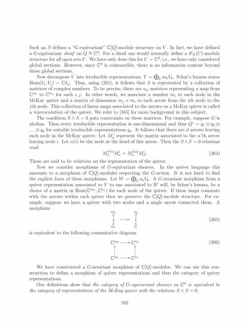
Such an S defines a “G-equivariant” C[Q]-module structure on V . In fact, we have defineda G-equivariant sheaf on Q ∼= Cd. For a sheaf one would normally define a OX(U)-modulestructure for all open sets U . We have only done this for U = Cd, i.e., we have only consideredglobal sections. However, since Cd is contractible, there is no information content beyondthese global sections.

Now decompose V into irreducible representations, V =⊕

k mkVk. Schur’s lemma statesHom(Vi, Vj) = Cδij. Thus, using (261), it follows that S is represented by a collection ofmatrices of complex numbers. To be precise, there are aij matrices representing a map fromCmi to Cmj for each i, j. In other words, we associate a number mi to each node in theMcKay quiver and a matrix of dimension mj ×mi to each arrow from the ith node to thejth node. This collection of linear maps associated to the arrows on a McKay quiver is calleda representation of the quiver. We refer to [165] for more background in this subject.

The condition S ∧ S = 0 puts constraints on these matrices. For example, suppose G isabelian. Then every irreducible representation is one-dimensional and thus Q∗ = q1 ⊕ q2 ⊕. . .⊕ qd for suitable irreducible representations qα. It follows that there are d arrows leavingeach node in the McKay quiver. Let M i

α represent the matrix associated to the α’th arrowleaving node i. Let α(i) be the node at the head of this arrow. Then the S ∧S = 0 relationsread

Mα(i)β M i

α = Mβ(i)α M i

β . (264)

These are said to be relations on the representation of the quiver.Now we consider morphisms of G-equivariant sheaves. In the quiver language this

amounts to a morphism of C[Q]-modules respecting the G-action. It is not hard to findthe explicit form of these morphisms. Let W =

⊕

k nkVk. A G-invariant morphism from aquiver representation associated to V to one associated to W will, by Schur’s lemma, be achoice of a matrix in Hom(Cmk ,Cnk) for each node of the quiver. If these maps commutewith the arrows within each quiver then we preserve the C[Q]-module structure. For ex-ample, suppose we have a quiver with two nodes and a single arrow connected them. Amorphism

m1

m2

n1

n2

(265)

is equivalent to the following commutative diagram

Cm2 Cn2

Cm1 Cn1

(266)

We have constructed a G-invariant morphism of C[Q]-modules. We can use this con-struction to define a morphism of quiver representations and thus the category of quiverrepresentations.

Our definitions show that the category of G-equivariant sheaves on Cd is equivalent tothe category of representations of the McKay quiver with the relations S ∧ S = 0.

102

The category of representations of the McKay quiver (with relations) is an abelian cate-gory. Each quiver representation is associated to a vector space V as defined above. Kernelsand cokernels may easily be computed purely from this vector space structure. When westart to write down exact sequences we see a new interpretation of the arrows in a quiver asfollows. Note that

0

0

1

1

1

1

0

0,f (267)

is a short exact sequence of quiver representations where the map f ∈ Hom(C,C) = C canbe multiplication by any complex number. Let Fi be the quiver representation with nj = δij ,i.e., V is simply the irreducible representation Vi. Assuming there are no arrows beginningand ending on the same node, all the maps in Fi are obviously zero and so Fi specifies aunique object. The short exact sequence (267) represents an extension of F1 by F2. Thatis Ext1(F1, F2) = C. This easily generalizes to an arbitrary quiver to give the followingresult (even if relations are imposed): the number of arrows from node i to node j equals thedimension of Ext1(Fi, Fj). Thus the quiver is often called an “Ext quiver”.

The most impressive generalization of the McKay correspondence was given by Bridge-land, King and Reid (BKR) [166] who said the following.

Theorem 3 Suppose X is a smooth resolution (i.e., blow-up) of the orbifold Cd/G with Ga finite subgroup of SU(d) and d ≤ 3.42 Then the derived category D(X) is equivalent to thederived category of G-equivariant sheaves on Cd.

In other words, D(X) is equivalent to the derived category of McKay quiver representationsassociated to G with relations S ∧S = 0. Thus, whereas the original McKay correspondenceviewed the arrows in the Dynkin diagram (262) as something to do with the intersectiontheory of the components of the exceptional divisor, in the generalization to three dimensionsit is best to view the arrows as a statement about Ext’s in the derived category.

Of course, the appearance of the derived category in the latter version of the McKaycorrespondence is excellent news for B-brane physics! The blow-up of an orbifold singularityis viewed as a deformation of B + iJ and so should not affect the B-model. It immediatelyfollows that

B-branes on the orbifold Cd/G and open strings between them are describedby the derived category of McKay quiver representations (with relations).

It follows that we have a distinguished set of D-branes on the orbifold associated to theirreducible representations of G. These will be associated to the quivers representations Fi

above. These branes were dubbed fractional branes in [157].

42The only reason why this should fail for d > 3 is that smooth resolutions need not exist.

103

The BKR result gives a precise recipe for mapping between these two derived categoriesas follows. Consider the following diagram

Zq

p

Cd

γ

Xπ

Cd/G,

(268)

where Z is defined as the “fibre product” of X and Cd. That is, Z is the subspace of X×Cd

given by points (x, z) such that π(x) = γ(z). The map γ is the quotient by G and π is theblow-down. The maps p and q are then the obvious projections on the fibre product. BKRthen say that q∗p

∗ gives the desired equivalence between D(X) and the derived category ofG-equivariant sheaves on Cd. Note that we think of sheaves on X as trivially G-equivariant.The map p∗ then typically introduces some non-trivial G-action.

As an example, consider the skyscraper sheaf Ox on X for x at a point in X not fixed bythe G-action. Then p∗Ox will be a collection of |G| skyscraper sheaves on Z transformingin the regular representation of G. This pushes forward to Cd to give the same collection ofskyscraper sheaves. Clearly the global sections of this sheaf on Cd form the regular repre-sentation of G. Thus the 0-branes on X correspond to quivers for the regular representationof G.

This means that, for 0-branes, the integer mi attached to each node in the quiver rep-resentation is equal to the dimension of the corresponding irreducible representation. Thelocation of the 0-brane will be dictated by the matrices associated to the arrows of thequiver. Once we study the stability of these B-branes we will see that the moduli space ofsuch stable quiver representations is equal to X as expected.

It also follows that the 0-brane is always composed of a nontrivial sum of fractional branes(hence the name). We will see that, at the orbifold point, the 0-brane is always marginallystable against decay into this set of underlying fractional branes.

7.3.2 The Douglas–Moore construction

We arrived at quivers from the mathematical direction of the McKay correspondence. Whilethis is probably the best approach for seeing the appearance of the full derived categoryof quiver representations, there is a wonderfully direct physics way of seeing why quiversthemselves should appear in the context of D-Branes on orbifolds. This is due to Douglasand Moore [156].

Suppose our full ten-dimensional spacetime looks like R1,3×C3/G and we have a 3-branethat fills the space-like directions of R1,3 and so appears as a 0-brane in the C3/G directions.The world-volume theory of this 3-brane yields an N = 1 supersymmetric field theory inR1,3.

One should note that this theory may, for general D-branes, have anomalies. This isbecause of the RR flux generated by the D-brane — an issue we have been able to ignore upto this point. One can remove these anomalies by using more background RR fluxes along

104

the lines of [92]. See also [167] for discussion of when these theories can be anomaly-free.Actually all our discussion of this four-dimensional quantum field theory will essentially beclassical, so we will ignore this issue of anomalies.

The idea is that one can analyze this quantum field theory by analyzing a collectionof D-branes in C3 corresponding to the preimage of the quotient map, and then imposingG-invariance.

Suppose we have m D-branes at the origin of C3 transforming in the representation V ofG. Let ρV (g) represent the m×m matrix representing g ∈ G in this representation. The fieldtheory will have a U(m) gauge symmetry. Let A be the corresponding gauge connection.The action of G is given explicitly by

g(A) = ρV (g) ·A · ρV (g)−1 (269)

In other words, A transforms in the representation End(V ) = V ⊗ V ∗ and the G-invariantpart of this can be written HomG(V, V ). By Schur’s lemma, the resulting gauge group isU(m1)× U(m2)× . . ., where V =

⊕

k mkVk as in the last section.Before dividing by G, we have an N = 4 supersymmetric gauge theory in four dimensions.

The N = 4 gauge superfield contains three scalar fields Z which arise from the components ofthe ten-dimensional connection pointing in the C3 directions. These fields transform underG similarly to A except that G acts on the C3 directions too. This latter 3-dimensionalrepresentation is clearly Q from the previous section. So the Z’s transform in Q⊗ End(V ).In other words, theG-invariant subspace of invariant scalar fields is given by HomG(V,Q⊗V ).Thus, from (263), the Z’s play the role of the matrices associated to the arrows in a quiverrepresentation.

Finally, to obtain complete agreement with the last section, we need to find the commu-tation relations on the quiver. These arise from the superpotential of the N = 4 theory [168].If we write Zµ, µ = 1, 2, 3, for the three scalar fields (each transforming in the adjoint ofU(m)) corresponding to the 3 directions in C3, this superpotential may be written

W = Tr(Z1[Z2, Z3]). (270)

The critical points of this superpotential impose precisely the relations S ∧ S = 0 fromsection 7.3.1.

To recap, the N = 1 supersymmetric field theory in R1,3 is described by the McKayquiver representations of section 7.3.1. The integers mi describe the effective gauge group.The homomorphisms associated to the arrows are associated to “bifundamental” scalar fieldsZ transforming accordingly in this gauge group. Finally, the commutation relations on thequiver representation are given by the superpotential.

This Douglas–Moore construction of a D-brane world-volume is identical mathematicallyto a problem studied by Sardo Infirri [169,170]. In this case one studies translation-invariantG-equivariant holomorphic bundles on Q = Cd. Let the fibre of a vector bundle be given bya representation V of G. Then, for G-equivariance, the connection on this bundle transforms

105

yet again in HomG(V,Q⊗ V ). Let us write this connection in the form

d∑

µ=1

Zµdzµ − Z†µdzµ. (271)

The (2, 0)-part of the curvature is then [169]

∑

µ,ν

(

−∂Zµ

∂zν+ 1

2[Zµ, Zν ]

)

dzµ ∧ dzν . (272)

If we impose translation invariance we demand that the derivatives of Zµ vanish. Thecondition that the bundle be holomorphic then amounts to [Zµ, Zν ] = 0 which again imposesthe relations on the quiver representation.

Thus we have three interpretations for the quiver representation:

1. A G-equivariant sheaf.

2. The scalar fields in the world-volume of a D-brane on an orbifold.

3. A connection on a translation-invariant holomorphic G-equivariant vector bundle.

The fact that these descriptions coincide allow us to prove a fact about the gradings ofthe fractional branes at the orbifold point. The scalar fields Zµ in our world-volume theorymust arise as open string states in the worldsheet description. That is, they occur as certainExt’s between the D-branes. The Ext-quiver language immediately tells us, of course, thatthese scalars are actually associated to Ext1’s between the fractional branes. The discussionaround equation (176) and section 6.2.3 tells us that a scalar state associated with Ext1

is massless if and only if the ξ-gradings at the end of the string are equal. Thus we haveproven:

Theorem 4 The gradings are equal for all the fractional branes at the orbifold point.

A consequence of this theorem is, of course, that the central charges of fractional D-branes align to have the same arg at the orbifold point. We will see this explicitly in anexample in section 7.3.6.

It is worth noting that the quiver language may be used in more general cases thanorbifolds. So long as the gradings of a set of branes are aligned, their Ext-quiver willrepresent the field content of an N = 1 theory in four dimensions. This ties the derivedcategory picture into quiver-related work such as [167, 171–173] etc. Sadly we do not havethe space to expand on this relation further.

106

7.3.3 θ-stability

We have established that the category of topological B-branes for an orbifold Cd/G corre-sponds to the derived category of quiver representations with relations. Now we want toimpose the BPS condition again, that is, we want a stability condition. We already knowwhat the answer is — Π-stability. However, since we have a relatively simple description ofB-branes on an orbifold, we might expect there to be a simpler description of the stabilitycondition for the orbifold for a region of the moduli space of B + iJ around the orbifoldpoint (i.e., small blow-ups). In other words, we want something analogous to the way µ-stability was a good description near the large radius limit. The answer is called θ-stabilityas introduced by King [174]. This was studied in the context of D-branes in [117–119].

Both the Douglas–Moore D-brane world-volume picture and the Sardo Infirri picture ofa G-equivariant bundle yield the condition for a BPS state. As one might guess, in the G-equivariant bundle picture we simply impose the condition that the connection is Hermitian–Yang–Mills. In the D-brane language we are required to minimize the potential arising fromthe “D-terms” in the action. Either way, the condition for a BPS state becomes43

∑

i

[Zµ, Z†µ] = 0. (273)

In section 7.3.1 we saw that the regular representation of G should correspond to theskyscraper sheaf Ox. One can show [169] that the moduli space of Z’s associated to theregular representation that satisfy (273) is indeed given by Cd/G as expected.

Now we want to resolve the orbifold a little. This means that we want to deform ourproblem in such a way that the moduli space of Z’s associated to the regular representationbecomes X, a resolution of the orbifold. In the D-brane language one may do this by adding“Fayet–Iliopoulos” terms to the action [156,175,176]. One such term may be added for eachunbroken U(1) of the gauge group, i.e., one for each irreducible representation of G. Let uscall the coefficients of these terms ζi, where i is an index running over the irreps of G. Theequivalent deformation is seen in the Sardo Infirri picture as a deformation of a “momentmap” [169].

The result is that (273) becomes

∑

µ

[Zµ, Z†µ] = diag(ζ1, ζ1, . . . , ζ1

︸ ︷︷ ︸

dim(V1)

, ζ2, ζ2, . . . , ζ2︸ ︷︷ ︸

dim(V2)

, . . .). (274)

In the case that G is abelian and d = 3, Sardo Infirri proved that the resulting modulispace of the 0-brane is indeed a resolution of Cd/G (see also [175]). The case d = 2 and anarbitrary G was proven earlier by Kronheimer [177].

Since the blow-up of an orbifold singularity is obtained by a deformation of B + iJ , thisresolution should be produced by closed string marginal operators. To be precise, twisted

43Note that in order to define the Hermitian conjugate Z†µ we require an inner product on the representa-

tion. This is intrinsic in the quantum field theory but is “extra data” in the abstract quiver language.

107

closed string marginal operators. Twisted operators are labeled by conjugacy classes inG [155] which we denote C. Let φC be a twisted operator present in the topological A-modelfor closed strings for the conjugacy class C and consider a deformation of B + iJ producedby adding a term

aC

∫

Σ

d2z φC , (275)

to the action. Turning on the ζi’s should be equivalent to turning on some aC ’s which impliesthat φC should acquire a nonzero 1-point function in the D-brane background. This one-point function was computed in [156, 175]. The result is, at least in a linear approximationfor very small blow-ups

aC =∑

i

χi(C) ζi, (276)

where χi’s are the characters of the group G.The operator φ1 associated to the conjugacy class of the identity is the closed string

tachyon and is removed by the GSO projection. Thus we require that a1 = 0, i.e.,

∑

i

dim(Vi) ζi = 0. (277)

Thus condition is also imposed by (274) since a commutator must be traceless.So far we have discussed the effects of nonzero ζi’s on the 0-brane, i.e., regular representa-

tion of G. What about general representations? The set-up is essential identical except thatthe Zµ’s now transform in another representation of G. Let us consider the representationV =

⊕

imiVi. Then (274) is modified so that the right-hand side is a diagonal matrix witheach ζi appearing mi times. In this more general setting the condition (277) can prevent(274) from having a solution.

In D-brane world-volume language this means that we cannot find a solution which makesthe contribution of the D-term to the potential equal to zero. At first sight, this would appearto break supersymmetry. In fact, this is not the case as pointed out in [117]. If we simplyminimize the potential then a not-so-manifest N = 1 supersymmetry still exists implying wedo have a BPS state. We refer to [117] for more details. Suppose we minimize the potentialby setting

∑

µ

[Zµ, Z†µ] = diag(θ1, θ1, . . . , θ1

︸ ︷︷ ︸

m1

, θ2, θ2, . . . , θ2︸ ︷︷ ︸

m2

, . . .), (278)

for some real numbers θi. The potential is then given by

∑

i

(ζi − θi)2, (279)

which is minimized subject to the condition (277) by

θi = ζi −∑

j mjζj∑

j mj

. (280)

108

The equation (278) may be written in a more quiver-friendly way as follows. Let a bean arrow in the quiver with head h(a) and tail t(a). Let Za be the mh(a) × mt(a) matrixassociated with this arrow in a given quiver representation. Then (278) becomes

∑

h(a)=i

ZaZ†a −

∑

t(a)=i

Z†aZa = θi id . (281)

This is exactly the equation studied by King [174]. Fix a representation of the quiverassociated to a representation V =

⊕

imiVi of G. For any representation W =⊕

i niVi ofG we define

θ(W ) =∑

i

θini. (282)

Thus, by the tracelessness of (278), we see θ(V ) = 0. We say that the quiver representationis θ-stable if, for any nontrivial quiver subrepresentation associated to a representation Wof G, θ(W ) > 0. King proved the following

Theorem 5 A quiver representation satisfies (281) (with an inner product unique up toobvious automorphisms) if and only if it a direct sum of θ-stable representations.

Thus, very close to the orbifold point we have a stability condition expressed purely interms of quivers.

7.3.4 Periods

For the remainder of these lectures we will focus on a particular example of an orbifold ratherthan attempt to prove any general statements. The example is C3/Z3 where g generates Z3

and acts as g : (z1, z2, z3) 7→ (ωz1, ωz2, ωz3) for ω = exp(2πi/3). Much of the analysis ofD-branes on orbifolds has been done in this simplest example (e.g., [118, 157,159,175]).

Let Vi, i = 0, . . . , 2 be the one-dimensional irreducible representations of Z3 given byρ(g) = ωi. A representation V = ⊕imiVi is then associated to a quiver representation

m2

m1.

m0

(283)

As is well-known, this orbifold is resolved with an exceptional divisor E ∼= P2. In thiscase, X may be viewed as the total space of the line bundle corresponding to the sheafOE(−3).

The computation to compute the periods and thus the central charges can be done ina way very similar to that of the quintic. In this section we perform the computationscorresponding to section 7.1.1.

Similarly to the quintic, we have a one-dimensional moduli space of B + iJ that canbe viewed as a P1. One point on this P1 corresponds to the large radius limit where the

109

exceptional divisor E is infinitely large. At the other extreme, we have the orbifold pointwhere we have no blow-up. At a third point on the P1, which we denote P0, we have theanalogue of the “conifold point” where B+ iJ have a special value that makes the associatedconformal field theory singular. Again, as in the quintic, we may use mirror symmetry toanalyze this moduli space and the associated periods exactly, as was first done in [35].

The Picard–Fuch’s equation in question is given by

(

zd

dz

)3

Φ + 27z

(

zd

dz

)(

zd

dz+ 1

3

)(

zd

dz+ 2

3

)

Φ = 0. (284)

Clearly any constant solves this differential equation. Putting z = (3e−πiψ)−3 we may writea basis for the remaining solutions near ψ = 0 as:

j =1

2πi

∞∑

n=1

Γ(n3)ωnj

Γ(n + 1)Γ(1− n3)2

(3ψ)n, (285)

where ω = exp(2πi/3). Thus 1, 0 and 1 form a basis for the solutions of the Picard–Fuchs equation. The analytic continuation to a basis for small z (valid for | arg(z)| < π) isperformed similarly to section 7.1.1:

Φ0 = 1,

Φ1 =1

2πi· 3

2πi

∫Γ(3s)Γ(−s)Γ(1 + s)2

zs ds

=1

2πilog z +O(z)

= t

= 0,

Φ2 = − 1

4π2· −6

2πi

∫Γ(3s)Γ(−s)2

Γ(s+ 1)(e−πiz)s ds

= − 1

4π2(log z − iπ)2 − 5

12+O(z)

= t2 − t− 16

+O(e2πit)

= −23(0 −1),

(286)

where the mirror map is given by t =∫

CB+iJ = 1

2πilog(z)+O(z), and C is a P1 hyperplane

in E. The analogue of figure 1 for the C3/Z3 orbifold is given in figure 13. Note that theorbifold point lies at exactly B = J = 0.44

Now, using (155) and (191), we can compute the exact value for central charges. Forexample, consider the 4-branes OE(m) wrapping the exceptional divisor:

Z(OE(m)) = −(m+ 43)0 + 1

31 + 1

2m2 + 3

2m+ 4

3. (287)

44There is a false assumption in [35] which shifts B by 1

2. The correct argument appears in [178].

110

-1.5

-1

-0.5

0

0.5

1

1.5

2

2.5

3

-1.5 -1 -0.5 0 0.5 1 1.5

B

J

•ψ = 0,Orbifold

•P0, ψ = e2πi/3•

ψ = e4πi/3

• ψ = 1

Figure 13: Fundamental regions for the moduli space of the Z3-orbifold.

Consider the point P0 in the moduli space where ψ = 2πi/3 and we have a singular conformalfield theory. At P0 we have 0 = t = 1

2+ iJ0 where J0 ≈ 0.4628. From (285) the value

of 1 at P0 will clearly be equal to the value of 0 at ψ = 4πi/3, namely −12

+ iJ0. Thus0 − 1 = 1 at P0. It follows from (288) that OE(−1) becomes massless at P0. SimilarlyOE(−2) becomes massless at the point ψ = 4πi/3.

We will therefore assume that the singularity in the conformal field theory at P0 is causedby the stable B-brane OE(−1) becoming massless. This appears to be very similar to thestatement that OC(−1) became massless for the singular conformal field theory for the caseof the flop in section 7.2. In the latter case we reset our definitions so that OC becamemassless instead. We will do the same here to make the results prettier. In effect we shiftt 7→ t+ 1 so that (287) becomes

Z(OE(m)) = −(m+ 13)0 + 1

31 + 1

2m2 + 1

2m+ 1

3, (288)

and now OE becomes massless at P0.

111

7.3.5 Monodromy

In general orbifolds may exhibit a “quantum symmetry” which acts on a state twisted byg ∈ G by multiplication by q(g), where

q ∈ Hom(G,C∗). (289)

The group Hom(G,C∗) is thus the group of quantum symmetries. It is not hard to show thatthis is isomorphic to the abelianization of G, i.e., G/[G,G]. Yet another interpretation ofHom(G,C∗) is the group of one-dimensional representations of G where the group operationis the tensor product. Given a one-dimensional representation U of G we may act on the setof representations by U ⊗ −. This gives a symmetry of the McKay quiver and thus showsexactly how the quantum symmetries of an orbifold act on the category of D-branes.

It is manifest from (262) that the extended Dynkin diagram for E8 has no symmetriesand thus the quantum symmetry group associated to the binary icosahedral group is trivial.That is, there is no quantum symmetry for this orbifold. Thus, we cannot possibly usequantum symmetries as a tool for making general statements about orbifolds but they canbe very useful in examples. In particular, if G is abelian, the quantum symmetry group isisomorphic to G and it acts transitively on the nodes of the McKay quiver. In our case, thequantum symmetry group Z3 acts by rotating the McKay quiver by 2π/3.

In section 7.1.4 we analyzed the monodromy around the Gepner point and discoveredthat the quantum Z5 symmetry one might expect in this context was in fact broken in thederived category. In this section we will show that the quantum symmetry of an orbifold, atleast in our example, is not broken by the derived category.

Monodromy around the large radius limit corresponds to tensoring by OX(D) where Dis a divisor Poincare dual to the component of the Kahler form which is being taken to bevery large. Thus we require D to intersect C (the P1 hyperplane of E) in one point. To fitin with the notation used in the case of the quintic we will denote OX(D) by OX(1). Thisnotation is also consistent with the fact that OX(1) ⊗ OE = OE(1). Note that since thenormal bundle of E corresponds to OE(−3), the analogue of the exact sequence (85) is

0 OX(3) OX OE 0. (290)

The monodromy associated to the “conifold point” P0 must be associated to the fact thatOE becomes massless there. If K is the Fourier–Mukai transform associated to monodromyaround P0, then, comparing to (232) we would expect a transform

TK(F ) = Cone(

Hom(E ,F )⊗ Er

F), (291)

where E is now OE. This corresponds to

K =(E ∨ ⊠ E

rO∆X

), (292)

where E ∨ is the dual of E defined in the derived category as RHom(E ,OX). Thus, if G isthe transform associated to the orbifold point, we have

G =(E ∨(1) ⊠ E O∆X(1)

)

=(OE(−1)∨ ⊠ OE O∆X(1)

).

(293)

112

The computation proceeds in a way very similar to section 7.1.4 to yield

G⋆3 =(

OE(−1)∨ ⊠ Ω2E(2) OE(−2)∨ ⊠ ΩE(1) OE(−3)∨ ⊠ OE O∆X(3)

). (294)

Using (290) we see that O∨E is

(OX OX(−3)

)which is OE(−3)[−1]. We may then apply

the Beilinson sequence (246) for E ∼= P2 to yield

G⋆3 = Cone(O∆E[−1] O∆X(3)

)

= Cone((

O∆X(3) O∆X

)−→ O∆X(3)

)

= O∆X .

(295)

Thus G⋆3 is the identity on the nose with no shifts involved. The quantum Z3 symmetry istherefore preserved even at the level of the derived category.

We may apply the BKR map of section 7.3.1 to determine the relationship between quiverrepresentations and coherent sheaves. The McKay equivalence may of course be composedwith any autoequivalence of D(X) and still give an equivalence. This gives a degree ofambiguity to how we may associate the derived category of sheaves to the derived categoryof quivers. We refer to [164, 179] for further details on how to compute the correspondenceexactly. Let ∆m0m1m2

denote a quiver representation of the form (283) and consider the frac-tional branes F0 = ∆100, F1 = ∆010 and F2 = ∆001. A choice of the McKay correspondenceconsistent with our conventions is then given by

F0 = 0

0

1

= OE

F1 = 0

1

0

= ΩE(1)[1]

F2 = 1

0

0

= OE(−1)[2].

(296)

From the above analysis of G it is easy to show that

TG(OE) = ΩE(1)[1]

T 2G(OE) = Ω2

E(2)[2] = OE(−1)[2].(297)

Thus TG indeed corresponds to rotating the McKay quiver clockwise by 2πi/3 or, equivalently,by tensoring by the representation F1. Perhaps we should emphasize that this picture doesnot work if we were to assert that F2 = OE(−1) without the shift of 2 as is done in much ofthe literature.

We may easily generalize the quintic hypersurface and the orbifold computation aboveto other dimensions (i.e., degree d hypersurfaces in Pd−1 and orbifolds Cn/Zn). In each casethe quantum symmetry of the Landau–Ginzburg orbifold is broken to become a shift left

113

by two and the quantum symmetry of the geometrical orbifold is preserved. Based on thisrather limited set of examples it is tempting to conjecture that this is a general result for allGepner models and for all orbifolds Cd/G. It would be interesting to prove this, or at leaststudy some more examples.

7.3.6 Examples of stability

In the case of the quintic we used the large radius limit as our base point for determiningstability. In the case of the orbifold, we can use the quantum symmetry to use the orbifoldpoint as the base point. First note that from (286) (with t shifted by 1) and (296) we have

Z(F0) = 13(1−0 +1)

Z(F1) = 13(1−0 − 21)

Z(F2) = 13(1 + 20 +1).

(298)

Thus, at the orbifold point, the Fi’s all have central charge 13. This is not surprising as the

Z3 quantum symmetry cyclically permutes the Fi’s are so their physics must be identical atthe orbifold point. In particular, they must all have the same value of ξ — a fact we provedin general at the end of section 7.3.2. We may thus declare at the orbifold point that

ξ(F0) = ξ(F1) = ξ(F2) = 0. (299)

Given (285), to a linear approximation in ψ near the orbifold we therefore have

ξ(∆m0m1m2) = −c(−m0 −m1 + 2m2) Re(ψ) + (m0 − 2m1 +m2) Re(ωψ)

m0 +m1 +m2

= c

∑

imiζi∑

imi

,

(300)

for a positive constant c and we define the ζk by

ζk =√

3 Re(eπi6

(4k−1)ψ), (301)

so that

ζ0 + ζ1 + ζ2 = 0

ζ0 + ωζ1 + ω2ζ2 = 3√

32e

πi6 ψ

ζ0 + ω2ζ1 + ωζ2 = 3√

32e−

πi6 ψ.

(302)

Clearly this is the analogue of (276) and the ζ ’s we have just introduced here correspond tothose of section 7.3.3. Indeed, we may now explicitly show that θ-stability is a limiting formof Π-stability near the orbifold point. Suppose we have a short exact sequence of quiverrepresentations

0 n2

n1

n0

m2

m1

m0

m2−n2

m1−n1

m0−n0

0. (303)

114

Near the orbifold point, the ξ’s of these 3 D-branes will be very close to zero. Thus, by theway central charges add, the ξ of the middle entry in (303) must lie between the ξ’s of theother two. For Π-stability of the middle entry we draw the distinguished triangle

m2

m1

m0

m2−n2

m1−n1

m0−n0

[1]f

n2

n1

n0

(304)

and look for the condition for f to be tachyonic. From (300) this is precisely∑

i niζi∑

i ni

<

∑

imiζi∑

imi

, (305)

which, from (280) is equivalent to King’s θ-stability statement of section 7.3.3.This θ-stability formulation allows us to completely classify the stable irreducible B-

branes near the orbifold point. As mentioned in section 6.1.3, the irreducibility for an objectA amounts to Hom(A,A) = C. A quiver representation satisfying this condition is known asa “Schur representation”. The problem of finding such representations was discussed in [118].

Determining whether a quiver representation (with relations) is Schur is a purely algebraquestion but turns out to be fairly awkward. In many cases it is actually more convenientto use the BKR equivalence and rephrase the question in terms of coherent sheaves.

As an example of a non-Schur quiver representation, consider ∆211 with generic maps onthe arrows in the quiver. With some effort one can show that the short exact sequence

0 0

0

1

1

1

2

1

1

1

0, (306)

is split. This immediately implies that Hom(∆211,∆211) ⊃ C2. This fact becomes moreobvious when written in terms of sheaves. ∆111 is a 0-brane which is generically nowherenear the exceptional divisor E, whereas ∆100 is the 4-brane OE wrapping E. Thus ∆211 isa sum of two quite disjoint D-branes and is obviously reducible. Note that when the mapson the arrows are not generic this quiver presentation might actually be Schur. This wouldcorrespond to the 0-brane being on E leading to a possible irreducible bound state with the4-brane.

We will not attempt to explicitly provide a complete solution to the classification problemhere but some Schur representations of interest are ∆111, and ∆abc, where a, b, c is anypermutation of 0, 1, n for n ≤ 3.

The fractional branes Fk are obviously always stable near the orbifold point since theyhave no nontrivial subobject in the category of quiver representations. Let us next focus on

115

∆111, some of which correspond to 0-branes. The quiver

1 6=0

1

6=0

1

6=0

(307)

with at least one nonzero map between each pair of nodes is stable since there is no injectivemap from any possible subobject to it. According to the explicit computations in [169,170]such a quiver represents a 0-brane away from the exceptional divisor E (or orbifold point ifwe haven’t blown up). Indeed, one would expect that the stability of such a 0-brane shouldnot be affected by orbifold-related matters.

Now consider the following short exact sequence:

0 0

0

1

1

1

1

0

1

1

0

0. (308)

This ∆111 is stable against decay to ∆100 by θ-stability if ζ0 < 0. We also have the sequence

0 0

1

1

1

1

1

0

1

0

0

0, (309)

giving a further constraint ζ2 > 0 on the stability of this 0-brane. Thus this 0-brane is stablein 2π/3 wedge coming out of the orbifold point. After blowing-up a little into this wedge, this0-brane corresponds to a point on the exceptional divisor. Obviously a cyclic permutationof the zero to another edge of the quiver results in similar statements with the ζ ’s permutedaccordingly. Thus, all other quivers ∆111 are unstable in the wedge ζ2 > 0, ζ0 < 0 and donot correspond to 0-branes at all.

The quiver representations with zero maps on the left edge have a close connection tosheaves on E as can be seen as follows. The general representation ∆abc falls into the sequence

0 0

0

1

c

b

a

0

c

b

a−1

0 0, (310)

and thus we iterate

c

b

a

0 = Cone

(

c

b

a−1

0

[−1]OE

)

= Cone

(

c

b

a−2

0

[−1]O

⊕2E

)

= Cone

(

c

b

0

[−1]O

⊕aE

)

.

(311)

116

−iψ

•

•ΩE [1](1) massless

•OE massless

•OE(−1)[2] massless

ζ2 > 0, ζ0 < 0

ζ0 > 0, ζ1 < 0ζ1 > 0, ζ2 < 0

OC decays

Op decaysOp decays

∆101 decays

∆n10 decays

∆0n1 decays

Figure 14: Some lines of marginal stability for the Z3-orbifold.

Continuing this process yields

c

b

a

0 =(

OE(−1)⊕c ΩE(1)⊕b O⊕aE

)

, (312)

explicitly mapping this quiver representation into the derived category of coherent sheaveson X (or E). This is precisely Beilinson’s construction of sheaves on P2 [148] and thiscorrespondence was identified in [118]. Thus, quiver representations with zero maps on theleft edge are seen to be associated to D-branes on E. We will get a pure sheaf of course onlyif the cohomology of the complex in (312) is concentrated at one term.

We denote some lines of marginal stability for Π-stability in figure 14. In each case, thearrow denotes the direction you cross the line to cause the relevant object to decay. Naturallythis agrees with θ-stability near the origin. The figure shows the moduli space in the form ofthe complex (−iψ)-plane. We make this choice so that the picture is aligned with figure 13,i.e., the large radius limit is upwards. Note that the lines of marginal stability correspondingto Op, p ∈ E, (i.e., the corresponding ∆111 quivers above) follow the lines of constant arg(ψ)even when the non-perturbative effects of Π-stability are taken into account.

Some decays of note are the following:

117

1. OC : This sheaf fits into the exact sequence

0 OE(−1) OE OC 0, (313)

and thus decays by Π-stability in a way essentially identical to the 4-branes in thequintic as in section 7.1.2. Thus, these 2-branes are stable at large radius but decaybefore the orbifold point is reached. Note that (313) implies that, in the derivedcategory of quiver representations we have

OC = Cone(F2[−2]→ F0). (314)

That is, this D-brane is essentially a complex of quivers and cannot be written interms of a single quiver. In other words, it is not in the abelian category of quiverrepresentations. It is therefore consistent with our picture that it decays before we getclose to the orbifold point.

2. ∆101: Following the logic of section 7.1.3 we can now look for an “exotic” D-brane bytaking the “Serre dual” of (314). This gives Cone(F0[−1], F2), i.e., an extension of F0

by F2. This is precisely ∆101. As expected from section 7.1.3, these objects should notbe stable at large radius but can become stable as we shrink the exceptional divisordown. The line of marginal stability is shown in figure 14. Note that they do notactually become stable until we shrink down to, or beyond, the orbifold point. Theseobjects generically have nonzero maps along the left edge of the triangle and so arenot classified by Beilinson’s construction (312).

We see a nice complementarity between the D-branes ∆101 and OC. OC is an objectin the category of coherent sheaves but is a complex in terms of quivers. ∆101 isan object in the category of quiver representations but becomes an exotic complexCone(OE[−1],OE(−1)[2]) in the derived category of sheaves.

3. ∆n10: This fits into the sequence

0 0

0

1

0

1

n

0

1

n−1

0. (315)

The produces a decay as shown in figure 14. The identification (312) together with theshort exact sequence

0 ΩE(1) O⊕3E OE(1) 0, (316)

may be used to show that

∆210∼= OC(1)

∆310∼= OE(1).

(317)

118

These D-branes are therefore simply objects both in terms of sheaves and quivers. Itis not surprising therefore that they are both stable at large radius limit and near theorbifold point.

On the other hand ∆110 does not correspond to a simple sheaf since the complex in(312) has cohomology in more than one place. In this case we have a sequence

0 0

1

1

1

1

1

1

0

0

0, (318)

which makes ∆110 only marginally stable at the large radius limit.

4. ∆0n1: This is similar to the ∆n10 case and again we plot the line of marginal stabilityin figure 14. This time ∆011 corresponds to the ideal sheaf of a point IE,p[1] and isagain only marginally stable at the large radius limit.

Clearly the study of D-brane stability on orbifolds is a very interesting subject and wehave only just begun to scratch the surface. The results above, together with previousanalysis in the literature such as [118, 157, 159, 175] provide a good start to the analysis ofthe subject but much remains to be done.

8 Conclusion

We hope that the reader is convinced that the derived category program is essential forunderstanding D-branes on a Calabi–Yau threefold and thus, presumably, D-branes in anynontrivial spacetime.

The essential ingredient is the extension of the naıve concept of “branes” and “anti-branes” to grading branes by arbitrary integers. This inexorably leads one to discuss com-plexes and soon the whole machinery of the derived category becomes unavoidable. Whilethe mathematics involved in this story might look excessive at first sight, it is hard to imaginehow one would understand B-branes without using this language or essentially reinventingsomething identical.

Given this complexity of B-branes it is perhaps worrying to note that we still made somedrastic simplifications in these lectures. The most egregious is probably the assumption thatthe string coupling is zero and thus the mass of any D-brane is infinite (unless it’s zero!). Thenext step one might therefore wish for is the notion of “quantizing” the derived categorystory which presumably introduces many many more complications. Clearly our currentknowledge of D-brane physics remains relatively poor.

Acknowledgments

It is a pleasure to thank M. Douglas who provided many of the basic ideas involved in thederived category approach to D-branes and Π-stability, and with whom I collaborated on

119

this subject. I also thank my collaborators A. Lawrence, P. Horja and R. Karp. In additionI have had many useful conversations with T. Bridgeland, S. Katz, I. Melnikov, D. Morrison,R. Plesser, R. Thomas, and I. Zharkov. I would like to thank K. T. Mahanthappa andJ. Maldecena for organizing TASI-03 for which these lecture notes were primarily written.Much of the motivation for working on a review of this subject was also provided by the “IfI Only Had a Brane” seminar series at Duke organized by Owen Patashnick.

The author is supported in part by NSF grant DMS-0301476.

References

[1] V. Gates, E. Kangaroo, M. Roachcock, and W. C. Gall, The Super G-String, inM. Green and D. Gross, editors, “Unified String Theories”, pages 729–737, WorldScientific, Singapore, 1986.

[2] C. V. Johnson, D-Branes, Cambridge University Press, 2003.

[3] B. R. Greene, String Theory on Calabi–Yau Manifolds, in C. Efthimiou and B. Greene,editors, “Fields, Strings and Duality, TASI 1996”, pages 543–726, World Scientific,1997, hep-th/9702155.

[4] D. A. Cox and S. Katz, Mirror Symmetry and Algebraic Geometry, MathematicalSurveys and Monographs 68, AMS, 1999.

[5] P. Candelas, Lectures on Complex Manifolds, in “Superstrings 1987: Proceedingsof the 1987 Trieste Spring School on Superstrings Proceedings”, pages 1–88, WorldScientific, 1988.

[6] M. R. Douglas, Lectures on D-branes on Calabi-Yau manifolds, Prepared for ICTPSpring School on Superstrings and Related Matters, Trieste, Italy, 2-10 Apr 2001,http://www.ictp.trieste.it/~pub_off/lectures/lns007/Douglas/Douglas.pdf.

[7] M. R. Douglas, Dirichlet Branes, Homological Mirror Symmetry, and Stability, in“Proceedings of the International Congress of Mathematicians: Beijing 2002”, vol. III,pages 395–408, Higher Education Press, Beijing, 2003, math.AG/0207021.

[8] K. Hori, editor, Mirror Symmetry, Clay Mathematics Monographs 1, AMS, 2003.

[9] E. Witten, Mirror Manifolds and Topological Field Theory, in S.-T. Yau, editor,“Essays on Mirror Manifolds”, International Press, 1992, hep-th/9112056.

[10] J. Polchinski, String Theory I,II, Cambridge, 1998.

[11] L. J. Dixon, Some World-Sheet Properties of Superstring Compactifications,on Orb-ifolds and Otherwise, in G. Furlan et al., editors, “Superstrings, Unified Theories, andCosmology 1987”, pages 67–126, World Scientific, 1988.

120

[12] N. P. Warner, Lectures on N = 2 Superconformal Field Theories and SingularityTheory, in M. B. Green et al., editors, “Superstrings ’89 : Proceedings of the TriesteSpring School, 3-14 April 1989”, World Scientific, 1990.

[13] W. Boucher, D. Friedan, and A. Kent, Determinant Formulae and Unitarity for theN = 2 Superconformal Algebras in Two Dimensions or Exact Results on String Com-pactification, Phys. Lett. B172 (1986) 316–322.

[14] W. Lerche, C. Vafa, and N. P. Warner, Chiral Rings in N = 2 Superconformal Theories,Nucl. Phys. B324 (1989) 427–474.

[15] E. Witten, Phases of N = 2 Theories in Two Dimensions, Nucl. Phys. B403 (1993)159–222, hep-th/9301042.

[16] K. Hori, Linear Models of Supersymmetric D-Branes, hep-th/0012179.

[17] S. Hellerman, S. Kachru, A. Lawrence, and J. McGreevy, Linear Sigma Models forOpen Strings, hep-th/0109069.

[18] S. Hellerman and J. McGreevy, Linear Sigma Model Toolshed for D-Brane Physics,hep-th/0104100.

[19] E. Witten, Topological Sigma Models, Commun. Math. Phys. 118 (1988) 411–449.

[20] E. Witten, Topological Quantum Field Theory, Commun. Math. Phys. 117 (1988)353–386.

[21] P. Candelas, X. C. de la Ossa, P. S. Green, and L. Parkes, A Pair of Calabi–YauManifolds as an Exactly Soluble Superconformal Theory, Nucl. Phys. B359 (1991)21–74.

[22] P. S. Aspinwall and D. R. Morrison, Topological Field Theory and Rational Curves,Commun. Math. Phys. 151 (1993) 245–262, hep-th/9110048.

[23] M. Bershadsky, S. Cecotti, H. Ooguri, and C. Vafa, Kodaira-Spencer Theory of Gravityand Exact Results for Quantum String Amplitudes, Commun. Math. Phys. 165 (1994)311–428, hep-th/9309140.

[24] R. Gopakumar and C. Vafa, On the Gauge Theory/Geometry Correspondence, Adv.Theor. Math. Phys. 3 (1999) 1415–1443, hep-th/9811131.

[25] H. Ooguri and C. Vafa, Worldsheet Derivation of a Large N Duality, Nucl. Phys.B641 (2002) 3–34, hep-th/0205297.

[26] M. Green, J. Schwarz, and E. Witten, Superstring Theory, Cambridge UniversityPress, 1987, 2 volumes.

121

[27] B. R. Greene and M. R. Plesser, Duality in Calabi–Yau Moduli Space, Nucl. Phys.B338 (1990) 15–37.

[28] B. de Wit, P. G. Lauwers, and A. Van Proeyen, Lagrangians of N = 2 Supergravity— Matter Systems, Nucl. Phys. B255 (1985) 569–608.

[29] A. Strominger, Special Geometry, Commun. Math. Phys. 133 (1990) 163–180.

[30] P. Candelas and X. C. de la Ossa, Moduli Space of Calabi–Yau Manifolds, Nucl. Phys.B355 (1991) 455–481.

[31] D. S. Freed, Special Kahler Manifolds, Commun. Math. Phys. 203 (1999) 31–52,hep-th/9712042.

[32] D. R. Morrison, Mirror Symmetry and Rational Curves on Quintic Threefolds: AGuide For Mathematicians, J. Amer. Math. Soc. 6 (1993) 223–247, alg-geom/9202004.

[33] D. R. Morrison, Picard-Fuchs Equations and Mirror Maps for Hypersurfaces, inS.-T. Yau, editor, “Essays on Mirror Manifolds”, International Press, 1992, alg-geom/9202026.

[34] V. V. Batyrev, Variations of the Mixed Hodge Structure of Affine Hypersurfaces inAlgebraic Tori, Duke Math. J. 69 (1993) 349–409.

[35] P. S. Aspinwall, B. R. Greene, and D. R. Morrison, Measuring Small Distances inN = 2 Sigma Models, Nucl. Phys. B420 (1994) 184–242, hep-th/9311042.

[36] D. Gepner, Exactly Solvable String Compactifications on Manifolds of SU(N) Holon-omy, Phys. Lett. 199B (1987) 380–388.

[37] C. Vafa and N. Warner, Catastrophes and the Classification of Conformal Theories,Phys. Lett 218B (1989) 51–58.

[38] B. Greene, C. Vafa, and N. Warner, Calabi–Yau Manifolds and Renormalization GroupFlows, Nucl. Phys. B324 (1989) 371–390.

[39] P. S. Aspinwall, Minimum Distances in Non-Trivial String Target Spaces, Nucl. Phys.B431 (1994) 78–96, hep-th/9404060.

[40] I. V. Melnikov, M. R. Plesser, and S. Rinke, Supersymmetric Boundary Conditions forthe N=2 Sigma Model, hep-th/0309223.

[41] C. Albertsson, U. Lindstrom, and M. Zabzine, N = 1 Supersymmetric Sigma Modelwith Boundaries. I, Commun. Math. Phys. 233 (2003) 403–421, hep-th/0111161.

[42] U. Lindstrom and M. Zabzine, N = 2 Boundary Conditions for Non-Linear SigmaModels and Landau-Ginzburg Models, JHEP 02 (2003) 006, hep-th/0209098.

122

[43] K. Hori, A. Iqbal, and C. Vafa, D-branes and Mirror Symmetry, hep-th/0005247.

[44] J. Polchinski, S. Chaudhuri, and C. V. Johnson, Notes on D-Branes, hep-th/9602052.

[45] H. Ooguri, Y. Oz, and Z. Yin, D-branes on Calabi-Yau Spaces and their Mirrors, Nucl.Phys. B477 (1996) 407–430, hep-th/9606112.

[46] A. Kapustin and D. Orlov, Vertex Algebras, Mirror Symmetry, and D-Branes: TheCase of Complex Tori, hep-th/0010293.

[47] N. Hitchin, Lectures on Special Lagrangian Submanifolds, math.DG/9907034.

[48] E. Witten, Chern-Simons Gauge Theory as a String Theory, in H. Hofer et al., editors,“The Floer Memorial Volume”, pages 637–678, Birkhauser, 1995, hep-th/9207094.

[49] Y.-G. Oh, Floer Coholomology of Lagrangian Intersections and Pseudo-HolomorphicDisks I & II, Comm. Pure Appl. Math. 46 (1993) 949–1012.

[50] E. Witten, Bound States Of Strings And p-Branes, Nucl. Phys. B460 (1996) 335–350,hep-th/9510135.

[51] S. Kachru, S. Katz, A. E. Lawrence, and J. McGreevy, Open String Instantons andSuperpotentials, Phys. Rev. D62 (2000) 026001, hep-th/9912151.

[52] S. Kachru, S. Katz, A. E. Lawrence, and J. McGreevy, Mirror Symmetry for OpenStrings, Phys. Rev. D62 (2000) 126005, hep-th/0006047.

[53] A. Strominger, S.-T. Yau, and E. Zaslow, Mirror Symmetry is T-Duality, Nucl. Phys.B479 (1996) 243–259, hep-th/9606040.

[54] B. Keller, Introduction to A-infinity Algebras and Modules, Homology Homotopy Appl.3 (2001) 1–35, math.RA/9910179.

[55] T. Lada and J. Stasheff, Introduction to SH Lie Algebras for Physicists, Internat. J.Theor. Phys. 32 (1993) 1087–1103.

[56] K. Fukaya and P. Seidel, Floer Homology, A∞-Categories and Topological Field Theory,Lecture Notes in Pure and Appl. Math. 184 (1997) 9–32.

[57] M. Herbst, C. Lazaroiu, and W. Lerche, Superpotentials, A-infinity Relations andWDVV Equations for Open Topological Strings, hep-th/0402110.

[58] C. A. Weibel, An Introduction to Homological Algebra, Cambridge Stud. in Adv.Math. 38, Cambridge, 1994.

[59] E. Witten, Supersymmetry and Morse theory, J. Diff. Geom. 17 (1982) 661–692.

123

[60] A. Floer, Symplectic fixed points and holomorphic spheres, Comm. Math. Phys. (1989)575–611.

[61] K. Fukaya, Morse Homotopy and its Quantization, in “Geometric topology (Athens,GA, 1993)”, AMS/IP Stud. Adv. Math. 2.1, Amer. Math. Soc., 1997, http://

www.kusm.kyoto-u.ac.jp/~fukaya/fukaya.html.

[62] K. Fukaya, Morse Homotopy, A∞-Category, and Floer Homologies, Lecture Notes Ser.18 (1993) 1–102.

[63] E. Witten, The N-Matrix Model and Gauged WZW Models, Nucl. Phys. B371 (1992)191–245.

[64] A. Floer, A Relative Morse Index for Symplectic Action, Commun. Pure. App. Math.41 (1988) 393–407.

[65] P. Seidel, Graded Lagrangian Submanifolds, Bull. Soc. Math. France 128 (2000) 103–149, math.SG/9903049.

[66] K. Fukaya, Floer Homology and Mirror Symmetry I, in 23, editor, “Winter Schoolon Mirror Symmetry, Vector Bundles and Lagrangian Submanifolds (Cambridge, MA,1999)”, AMS/IP Stud. Adv. Math., pages 15–43, AMS, 2001.

[67] M. Kontsevich and Y. Soibelman, Homological Mirror Symmetry and Torus Fibrations,in K. Fukaya et al., editors, “Symplectic Geometry and Mirror Symmetry”, pages 203–263, World Scientific, 2001, math.SG/0011041.

[68] K. Fukaya, Y.-G. Oh, H. Ohta, and K. Ono, Lagrangian Intersection Floer The-ory — Anomaly and Obstruction, 2000, http://www.kusm.kyoto-u.ac.jp/~fukaya/fukaya.html.

[69] A. Polishchuk and E. Zaslow, Categorical Mirror Symmetry: The Elliptic Curve, Adv.Theor. Math. Phys. 2 (1998) 443–470, math.AG/9801119.

[70] A. Polishchuk, A∞-Structures on an Elliptic Curve, math.AG/0001048.

[71] P. Seidel, Homological Mirror Symmetry for the Quartic Surface, math.SG/0310414.

[72] S. Merkulov, Strongly Homotopy Algebras of a Kahler Manifold, Internat. Math. Res.Notices (1999) 153–164, math.AG/9809172.

[73] M. Kontsevich, Homological Algebra of Mirror Symmetry, in “Proceedings of theInternational Congress of Mathematicians”, pages 120–139, Birkhauser, 1995, alg-geom/9411018.

[74] R. Hartshorne, Algebraic Geometry, Graduate Texts in Mathematics 52, Springer-Verlag, 1977.

124

[75] M. Kashiwara and P. Schapira, Sheaves on Manifolds, Springer, 1990.

[76] A. Grothendieck, Sur le classification de fibres holomorphes sur le sphere de Riemann,Am. J. Math. 79 (1957) 121–138.

[77] P. Freyd, Abelian Categories, Harper and Row, 1964.

[78] P. Griffiths and J. Harris, Principles of Algebraic Geometry, Wiley-Interscience, 1978.

[79] R. Bott and L. W. Tu, Differential Forms in Algebraic Topology, Springer-Verlag, NewYork, 1982.

[80] J. McCleary, User’s Guide to Spectral Sequence, Publish or Perish, 1985.

[81] S. I. Gelfand and Y. I. Manin, Homological Algebra, Encyclopædia of MathematicalSciences 38, Springer, 1994.

[82] P. S. Aspinwall and A. E. Lawrence, Derived Categories and Zero-Brane Stability,JHEP 08 (2001) 004, hep-th/0104147.

[83] M. R. Douglas, D-Branes, Categories and N=1 Supersymmetry, J. Math. Phys. 42

(2001) 2818–2843, hep-th/0011017.

[84] D. S. Freed and E. Witten, Anomalies in String Theory with D-branes, hep-th/9907189.

[85] S. Katz and E. Sharpe, D-branes, Open String Vertex Operators, and Ext Groups,Adv.Theor.Math.Phys. 6 (2003) 979–1030, hep-th/0208104.

[86] E. Sharpe, Lectures on D-branes and Sheaves, hep-th/0307245.

[87] R. P. Thomas, Derived Categories for the Working Mathematician, math.AG/0001045.

[88] J. Morrow and K. Kodaira, Complex Manifolds, Holt, Rinehart and Winston, 1971.

[89] A. Sen, Tachyon Condensation on the Brane Antibrane System, JHEP 08 (1998) 012,hep-th/9805170.

[90] E. Witten, D-branes and K-Theory, J. High Energy Phys. 12 (1998) 019, hep-th/9810188.

[91] E. Sharpe, D-branes, Derived Categories, and Grothendieck Groups, Nucl. Phys. B561

(1999) 433–450, hep-th/9902116.

[92] M. Green, J. A. Harvey, and G. Moore, I-brane Inflow and Anomalous Couplings onD-Branes, Class. Quant. Grav. 14 (1997) 47–52, hep-th/9605033.

[93] Y.-K. E. Cheung and Z. Yin, Anomalies, Branes, and Currents, Nucl. Phys. B517

(1998) 69–91, hep-th/9710206.

125

[94] R. Minasian and G. Moore, K-Theory and Ramond-Ramond Charge, J. High EnergyPhys. 11 (1997) 002, hep-th/9710230.

[95] J. A. Harvey, TASI 2003 Lectures on Anomalies, to appear.

[96] R. P. Thomas, An obstructed bundle on a Calabi-Yau 3-fold, Adv. Theor. Math. Phys.3 (1999) 567–576, math.AG/9903034.

[97] P. M. H. Wilson, The Kahler Cone on Calabi–Yau Threefolds, Invent. Math. 107

(1992) 561–583.

[98] F. Denef, Supergravity Flows and D-brane Stability, JHEP 08 (2000) 050, hep-th/0005049.

[99] F. Denef, B. Greene, and M. Raugas, Split Attractor Flows and the Spectrum of BPSD-branes on the Quintic, JHEP 05 (2001) 012, hep-th/0101135.

[100] K. Becker, M. Becker, and A. Strominger, Five-branes, Membranes and Nonperturba-tive String Theory, Nucl. Phys. B456 (1995) 130–152, hep-th/9507158.

[101] R. Harvey and H. B. Lawson, Calibrated Geometries, Acta Mathematica 148 (1982)47–157.

[102] R. C. McLean, Deformations of Calibrated Submanifolds, Comm. Anal. Geom. 6

(1998) 705–747.

[103] D. Joyce, Special Lagrangian Submanifolds with Isolated Conical Singularities. V.Survey and Applications, math.DG/0303272.

[104] M. Berkooz, M. R. Douglas, and R. G. Leigh, Branes Intersecting at Angles, Nucl.Phys. B480 (1996) 265–278, hep-th/9606139.

[105] G. Lawlor, The Angle Criterion, Invent. Math. 95 (1989) 437–446.

[106] R. Harvey, Spinors and Calibrations, Academic Press, 1990.

[107] S. P. Marshall, Deformations of Special Lagrangians, 2002, Oxford DPhil thesis.

[108] N. Seiberg and E. Witten, Electric - Magnetic Duality, Monopole Condensation, andConfinement in N=2 Supersymmetric Yang-Mills Theory, Nucl. Phys. B426 (1994)19–52, hep-th/9407087, (erratum-ibid. B430 (1994) 485-486).

[109] W. Lerche, Introduction to Seiberg–Witten Theory and its Stringy Origin, Nucl. Phys.Proc. Suppl. 55B (1997) 83–117, hep-th/9611190.

[110] W. Taylor and B. Zwiebach, D-branes, Tachyons, and String Field Theory, hep-th/0311017.

126

[111] R. P. Thomas, Moment Maps, Monodromy and Mirror Manifolds, in K. Fukayaet al., editors, “Symplectic Geometry and Mirror Symmetry”, pages 467–498, WorldScientific, 2001, math.DG/0104196.

[112] R. P. Thomas and S.T.-Yau, Special Lagrangians, Stable Bundles and Mean CurvatureFlow, Commun. Anal. Geom. 10 (2002) 1075–1113, math.DG/0104197.

[113] S. MacLane, Homology, Springer, 1975.

[114] J.-L. Verdier, Categories derivees, etat 0, Lecture Notes in Math. 569, Spinger, 1977.

[115] A. I. Bondal and M. M. Kapranov, Framed Triangulated Categories, Math. USSR-Sb.70 (1991) 93–107.

[116] M. T. Grisaru, A. van de Ven, and D. Zanon, Two-Dimensional SupersymmetricSigma-Models on Ricci-Flat Kahler Manifolds are Not Finite, Nucl. Phys. B277 (1986)388–408.

[117] M. R. Douglas, B. Fiol, and C. Romelsberger, Stability and BPS Branes, hep-th/0002037.

[118] M. R. Douglas, B. Fiol, and C. Romelsberger, The Spectrum of BPS Branes on aNoncompact Calabi-Yau, hep-th/0003263.

[119] B. Fiol and M. Marino, BPS States and Algebras from Quivers, JHEP 07 (2000) 031,hep-th/0006189.

[120] P. S. Aspinwall and M. R. Douglas, D-Brane Stability and Monodromy, JHEP 05

(2002) 031, hep-th/0110071.

[121] A. Strominger, Massless Black Holes and Conifolds in String Theory, Nucl. Phys.B451 (1995) 96–108, hep-th/9504090.

[122] B. R. Greene, D. R. Morrison, and A. Strominger, Black Hole Condensation and theUnification of String Vacua, Nucl. Phys. B451 (1995) 109–120, hep-th/9504145.

[123] T. Bridgeland, Stability Conditions on Triangulated Categories, math.AG/0212237.

[124] T. Bridgeland, Stability Conditions on K3 Surfaces, math.AG/0307164.

[125] M. Marino, R. Minasian, G. W. Moore, and A. Strominger, Nonlinear Instantons fromSupersymmetric p-Branes, JHEP 01 (2000) 005, hep-th/9911206.

[126] K. Uhlenbeck and S.-T. Yau, On the Existence of Hermitian Yang-Mills Connectionsin Stable Vector Bundles, Commun. Pure App. Math. 39 (1986) S257–S293.

[127] S. Donaldson, Anti-Self-Dual Yang-Mills Connections on Complex Algebraic Surfacesand Stable Vector Bundles, Proc. London Math Soc. 50 (1985) 1–26.

127

[128] M. R. Douglas, D-Branes and N=1 Supersymmetry, hep-th/0105014.

[129] A. Recknagel and V. Schomerus, D-branes in Gepner Models, Nucl. Phys. B531

(1998) 185–225, hep-th/9712186.

[130] I. Brunner, M. R. Douglas, A. Lawrence, and C. Romelsberger, D-branes on theQuintic, JHEP 08 (2000) 015, hep-th/9906200.

[131] J. Fuchs, C. Schweigert, and J. Walcher, Projections in String Theory and BoundaryStates for Gepner Models, Nucl. Phys. B588 (2000) 110–148, hep-th/0003298.

[132] A. Kapustin and Y. Li, Topological Correlators in Landau–Ginzburg Models withBoundaries, hep-th/0305136.

[133] A. Kapustin and Y. Li, D-Branes in Topological Minimal Models: The Landau–Ginzburg Approach, hep-th/0306001.

[134] S. K. Ashok, E. Dell’Aquila, and D.-E. Diaconescu, Fractional Branes in Landau-Ginzburg Orbifolds, hep-th/0401135.

[135] D. Orlov, Equivalences of Derived Categories and K3 Surfaces., J. Math. Sci. 87

(1997) 1361–1381, alg-geom/9606006.

[136] T. Bridgeland, Equivalences of Triangulated Categories and Fourier–Mukai Trans-forms, Bull. London Math. Soc. 31 (1999) 25–34, math.AG/9809114.

[137] S. Govindarajan and T. Jayaraman, D-branes, Exceptional Sheaves and Quivers onCalabi–Yau Manifolds: From Mukai to McKay, Nucl. Phys. B600 (2001) 457–486,hep-th/0010196.

[138] A. Tomasiello, D-branes on Calabi-Yau Manifolds and Helices, JHEP 02 (2001) 008,hep-th/0010217.

[139] P. Mayr, Phases of Supersymmetric D-branes on Kahler Manifolds and the McKayCorrespondence, JHEP 01 (2001) 018, hep-th/0010223.

[140] T. Bridgeland and A. Maciocia, Fourier-Mukai transforms for Quotient Varieties,math.AG/9811101.

[141] S. A. Kuleshon and D. O. Orlov, Exceptional Sheaves on Del Pezzo Surfaces, RussianAcad. Sci. Izv. Math. 44 (1995) 479–513.

[142] M. Kontsevich, 1996, Rutgers Lecture, unpublished.

[143] P. Seidel and R. P. Thomas, Braid Groups Actions on Derived Categories of CoherentSheaves, Duke Math. J. 108 (2001) 37–108, math.AG/0001043.

128

[144] R. P. Horja, Hypergeometric Functions and Mirror Symmetry in Toric Varieties,math.AG/9912109.

[145] R. P. Horja, Derived Category Automorphisms from Mirror Symmetry, math.AG/-0103231.

[146] P. S. Aspinwall, R. P. Horja, and R. L. Karp, Massless D-Branes on Calabi–YauThreefolds and Monodromy, hep-th/0209161.

[147] W. Fulton and J. Harris, Representation Theory: A First Course, Springer-Verlag,1991.

[148] A. A. Beilinson, Coherent Sheaves on Pn and Problems in Linear Algebra, Func. Anal.Appl. 12 (1978) 214–216.

[149] D. Orlov, Triangulated Categories of Singularities and D-Branes in Landau–GinzburgOrbifolds, math.AG/0302304.

[150] P. S. Aspinwall, B. R. Greene, and D. R. Morrison, Calabi–Yau Moduli Space, MirrorManifolds and Spacetime Topology Change in String Theory, Nucl. Phys. B416 (1994)414–480.

[151] P. S. Aspinwall, A Point’s Point of View of Stringy Geometry, JHEP 01 (2003) 002,hep-th/0203111.

[152] T. Bridgeland, Flops and Derived Categories, math.AG/0009053.

[153] R. Hartshorne, Residues and Duality, Lecture Notes in Math. 20, Spinger-Verlag,1966.

[154] A. Bondal and D. Orlov, Semiorthogonal Decomposition for Algebraic Varieties, alg-geom/9506012.

[155] L. Dixon, J. A. Harvey, C. Vafa, and E. Witten, Strings on Orbifolds, Nucl. Phys.B261 (1985) 678–686, and B274 (1986) 285–314.

[156] M. R. Douglas and G. Moore, D-branes, Quivers, and ALE Instantons, hep-th/9603167.

[157] D.-E. Diaconescu, M. R. Douglas, and J. Gomis, Fractional Branes and WrappedBranes, JHEP 02 (1998) 013, hep-th/9712230.

[158] D.-E. Diaconescu and M. R. Douglas, D-branes on Stringy Calabi–Yau Manifolds,hep-th/0006224.

[159] D.-E. Diaconescu and J. Gomis, Fractional Branes and Boundary States in OrbifoldTheories, JHEP 10 (2000) 001, hep-th/9906242.

129

[160] W. Lerche, P. Mayr, and J. Walcher, A New Kind of McKay Correspondence fromNon-Abelian Gauge Theories, hep-th/0103114.

[161] P. S. Aspinwall, Resolution of Orbifold Singularities in String Theory, in B. Greeneand S.-T. Yau, editors, “Mirror Symmetry II”, pages 355–426, International Press,1996, hep-th/9403123.

[162] J. McKay, Graphs, Singularities and Finite Groups, Proc. Symp. Pure Math. 37

(1980) 183–186.

[163] P. S. Aspinwall, K3 Surfaces and String Duality, in C. Efthimiou and B. Greene,editors, “Fields, Strings and Duality, TASI 1996”, pages 421–540, World Scientific,1997, hep-th/9611137.

[164] A. Craw and A. Ishii, Flops of G-Hilb and Equivalences of Derived Categories byVariation of GIT Quotient, math.AG/0211360.

[165] D. J. Benson, Representations and Cohomology: I, Cambridge, 1991.

[166] T. Bridgeland, A. King, and M. Reid, Mukai implies McKay, J. Amer. Math. Soc. 14

(2001) 535–554, math.AG/9908027.

[167] F. Cachazo et al., A Geometric Unification of Dualities, Nucl. Phys. B628 (2002)3–78, hep-th/0110028.

[168] L. Brink, J. H. Schwarz, and J. Scherk, Supersymmetric Yang-Mills Theories, Nucl.Phys. B121 (1977) 77–92.

[169] A. V. Sardo Infirri, Partial Resolutions of Orbifold Singularities via Moduli Spaces ofHYM-type Bundles, alg-geom/9610004.

[170] A. V. Sardo Infirri, Resolutions of Orbifold Singularities and the Transportation Prob-lem on the McKay Quiver, alg-geom/9610005.

[171] M. Wijnholt, Large Volume Perspective on Branes at Singularities, hep-th/0212021.

[172] C. P. Herzog and J. Walcher, Dibaryons from Exceptional Collections, JHEP 09 (2003)060, hep-th/0306298.

[173] C. P. Herzog, Exceptional Collections and del Pezzo Gauge Theories, hep-th/0310262.

[174] A. D. King, Moduli of Representations of Finite Dimensional Algebras, Quart. J.Math. Oxford (2) 45 (1994) 515–530.

[175] M. R. Douglas, B. R. Greene, and D. R. Morrison, Orbifold Resolution by D-Branes,Nucl. Phys. B506 (1997) 84–106, hep-th/9704151.

130

[176] B. R. Greene, C. I. Lazaroiu, and M. Raugas, D-branes on Nonabelian ThreefoldQuotient Singularities, Nucl. Phys. B553 (1999) 711–749, hep-th/9811201.

[177] P. Kronheimer, The Construction of ALE Spaces as Hyper-Kahler Quotients, J. Diff.Geom. 29 (1989) 665–683.

[178] D. R. Morrison and M. R. Plesser, Summing the Instantons: Quantum Cohomologyand Mirror Symmetry in Toric Varieties, Nucl. Phys. B440 (1995) 279–354, hep-th/9412236.

[179] S. Katz, T. Pantev, and E. Sharpe, D-branes, Orbifolds, and Ext Groups, Nucl. Phys.B673 (2003) 263–300, hep-th/0212218.

131