Czech Technical University in Prague Faculty of Nuclear ...
77
Czech Technical University in Prague Faculty of Nuclear Sciences and Physical Engineering Department of Physics Physics and Technology of Nuclear Fusion Ubíhající elektrony v tokamaku a jejich detekce Runaway electrons in the tokamak and their detection Diploma thesis Author: Bc. Lenka Kocmanová Supervisor: Mgr. Richard Papřok Consultant: RNDr. Jan Stöckel, CSc. 1
Transcript of Czech Technical University in Prague Faculty of Nuclear ...

Czech Technical University in Prague
Faculty of Nuclear Sciences and Physical Engineering
Department of Physics
Physics and Technology of Nuclear Fusion
Ubíhající elektrony v tokamaku a jejich detekce
Runaway electrons in the tokamak and their detection
Diploma thesis
Author: Bc. Lenka Kocmanová
Supervisor: Mgr. Richard Papřok
Consultant: RNDr. Jan Stöckel, CSc.
1

České vysoké učení technické v Praze
Fakulta jaderná a fyzikálně inženýrská v PrazeKatedra fyziky
Aplikace přírodních věd
Fyzika a technika termojaderné fúze
Ubíhající elektrony v tokamaku a jejich detekce
Runaway electrons in the tokamak and their detection
Diplomová práce
Vypracovala: Bc.Lenka Kocmanová
Vedoucí práce: Mgr. Richard Papřok
Konzultant: RNDr. Jan Stöckel, CSc.
2

Prohlášení
Prohlašuji, že jsem diplomovou práci vypracovala samostatně a použila jsem pouze podklady uvedené v přiloženém seznamu.
Nemám závažný důvod proti užití tohoto školního díla ve smyslu § 60 Zákona č.121/2000 Sb., o právu autorském, o právech souvisejících s právem autorským a o změně některých zákonů (autorský zákon).
V Praze dne ….......................
…............................................
Bc. Lenka Kocmanová
3

Acknowledgements
I would like to thank Richard Papřok for his supervision and useful comments on the work. I thank also Jan Stöckel for helpful discusions on the experimental part.
4

Název práce: Ubíhající elektrony v tokamaku a jejich detekce
Autor: Bc. Lenka Kocmanová
Obor: Aplikace přírodních věd
Druh práce: Diplomová práce
Vedoucí práce: Mgr. Richard Papřok, Ústav fyziky plazmatu, AV,ČR, v.v.i.
Konzultant: RNDr. Jan Stöckel, CSc., Ústav fyziky plazmatu, AV,ČR, v.v.i.
Klíčová slova: tokamak, ubíhající elektrony, tvrdé rentgenové záření, scintilační sonda
Abstrakt: Diplomová práce se zabývá fyzikou ubíhajících elektronů v tokamaku a zpracováním jejich měření na tokamacích GOLEM a COMPASS. V teoretické části definuji ubíhající elektrony, zabývám se jejich rovnicemi pohybu. Věnuji se rozvoji rychlosti elektronu ve 2D rychlostním prostoru. Dále jsou popsány radiační ztráty. V druhé části je zpracované měření tvrdého rentgenového záření, jejichž zdrojem je dopad ubíhajících elektronů na stěnu tokamaku.
Title: Runaway electrons in the tokamak and their detection
Key words: tokamak, runaway electrons, hard x-ray, scintillator
Abstract: The diploma thesis is deal with runaway electrons. The project has two major parts, theoretical descriptions and measurement. The definitions of runaway electrons are included. The electron motion is divided into full equations of motion and gyrocenter equations of motion. A electron motion is described. 2D velocity space and radiation losses of runaway electrons are also depisted. Some numerical codes which calculate parameters important for runaway electrons are mentioned. The measurement on GOLEM and COMPASS tokamaks is included in the practical part. We used scintillator detector for detection HXR. Photons are produced when the runaway electron hit the plasma facing components.
5

Table of Contents 1 Basic informations about runaway electrons...................................................................................9
1.1 Tokamak...................................................................................................................................9 1.2 Practical Motivation for study of Runaway electrons...........................................................10 1.3 Creation mechanisms ............................................................................................................11
1.3.1 Mitigation methods........................................................................................................13 2 Motion of test particle...................................................................................................................15
2.1 Full equations of motion........................................................................................................15 2.2 Gyro-center equations of motion...........................................................................................15 2.3 Drifts of particles in magnetized plasma...............................................................................16 2.4 Constants of motion...............................................................................................................17 2.5 Drift orbits..............................................................................................................................18 2.6 Dynamics and momentum space...........................................................................................21 2.7 Particle orbits - When is particle trapped or passing?...........................................................24
3 Terms in bounce averaged kinetic equation .................................................................................25 3.1 The collision operator...........................................................................................................25 3.2 Collision operator in a comparison with the other paper.......................................................29 3.3 Runaway rate.........................................................................................................................29
4 Radiation losses ............................................................................................................................32 4.1 Conditions for consideration of radiation..............................................................................32 4.2 From Abraham-Lorentz equation to effect of radiation reaction...........................................33 4.3 Comparison of [14] with [11]...............................................................................................34 4.4 Angle dependence..................................................................................................................34
4.4.1 Synchrotron radiation.....................................................................................................34 4.4.2 Bremsstrahlung............................................................................................................36
5 Some Analytical Estimates ...........................................................................................................39 5.1 Number of runaway electrons................................................................................................39 5.2 Dependence of the runaway rate on a plasma density...........................................................42 5.3 Comparision of influence of collisional slowing, synchrotron and bremsstrahlung drag.....43 5.4 Outward drift velocity............................................................................................................45 5.5 HXR emission .......................................................................................................................46
6 Numerical Codes used in Runaway electron physics....................................................................48 6.1 Particle tracking codes ..........................................................................................................48 6.2 Bounce averaged kinetic equation.........................................................................................48 6.3 Focker Plank solver...............................................................................................................49 6.4 Coupling of Particle tracking codes to MHD codes..............................................................50
7 Experimental part .........................................................................................................................51 7.1 Measurement of the HXR emission on the GOLEM tokamak..............................................51
7.1.1 GOLEM tokamak...........................................................................................................51 7.1.2 Experimental setup.........................................................................................................51
7.1.2.1 Properties of scintillator detector...........................................................................51 7.1.2.2 Calibration..............................................................................................................52
7.1.3 Results............................................................................................................................53 7.1.3.1 Dependence on magnetic field...............................................................................54 7.1.3.2 Dependence on temperature...................................................................................59
7.1.4 COMPASS tokamak.......................................................................................................61 7.1.5 Experiment setup............................................................................................................62
6

7.1.6 Typical energy spectrum of HXR photons.....................................................................62 7.1.6.1 Comparison with the non-calibrated HXR detector ..............................................65
7.1.7 Discusion........................................................................................................................67 8 Conclusion.....................................................................................................................................69 9 Appendix .......................................................................................................................................72
9.1 Lagrangian and Hamiltonian.................................................................................................72 9.2 Relativistic Lagrangian and Hamiltonian..............................................................................73
10 References...................................................................................................................................76
7

Introduction
Humanity is going to wrestle with a deficiency of energy in few decades.[1] The most reasonable solution is a fusion. At the heart of a star, fusion occurs when hydrogen atoms fuse together under extreme heat and pressure to create a denser helium atom releasing, in the process, colossal amounts of energy. But on Earth, scientists have to try and replicate a star's intense gravitational pressure with an artificial magnetic field that requires huge amounts of electricity. Fusion has lot of positive properties. Fusion doesn't produce greenhouse gases, it is intrinsically safe and it leaves no burden on future generations. The primary reaction does not produce nuclear material, only helium. There's a limited problem in that you produce neutrons, but this only makes the reactor chamber itself radioactive. Within 100 years, it could be recycled the chamber so there's no need for geological-timescale storage as there is with the waste from fission energy. And the fuel is virtually unlimited. There is needed only lithium and hydrogen. Sea water alone could fuel current human consumption levels for 30 million years. By 2019, it is hoped that the world's largest and most advanced experimental tokamak will be switched on. The International Thermonuclear Experimental Reactor (ITER), which will cost 15 bilion Euros, is being funded by an unprecedented international coalition, including the EU, the US, China, India, South Korea and Russia. The ITER will demonstrate the commercial viability of fusion by producing a tenfold power gain of 500MW during shots lasting up to an hour. If the ITER will accomplish anticipation a demonstration plant DEMO will be built. It should be built by 2040.
8
1 Basic informations about runaway electronsIn this chapter a tokamak description is adduced. Basic needed definitions and reasons for study the runaway electrons are mentioned here.
1.1 Tokamak
The tokamak is a toroidal plasma confinement system, the plasma being confined by a magnetic field.[2] The principal magnetic field is the toroidal field. This field alone does not allow confinement of the plasma. In order to have an equilibrium in which the plasma pressure is balanced by magnetic field forces it is necessary also to have a poloidal magnetic field. In a tokamak this field is produced mainly by current in the plasma itself, this current flowing in toroidal direction. The combination of the toroidal field and poloidal field gives rise to magnetic field lines which have a helical trajectory around the torus. The toroidal magnetic field is produced by currents in coils linking the plasma.
The plasma pressure is the product of the particle density and temperature. The fact that the reactivity of the plasma increases with both of these quantities implies that in a reactor the pressure must be sufficiently high. The pressure which can be confined is determined by stability considerations and increases with the strength of the magnetic field. The magnitude of the toroidal field is limited by technological factors. The requirement for cooling and the magnetic forces put a limit on the magnetic field which they can produce. There are needed superconducting coils. A loss of superconductivity occurs above a critical magnetic field and this presents another limitation. With present technology it seems likely that the maximum magnetic field at the coils would be limited. The maximum toroidal field appears at the inboard side of the toroidal field coil. The toroidal magnetic field is inversely proportional to the major radius.
For a given toroidal magnetic field the plasma pressure which can be stably confined increases with toroidal plasma current up to a limiting value. The resulting poloidal magnetic field are typically an order of magnitude smaller than the toroidal field.
In present experiments the plasma current is driven by a toroidal electric field induced by transformer action in which a flux change is generated though the torus. The flux change is brought about by a current passed through a primary coil around the torus.
There are advantages for confinement and achievable pressure with plasmas which are vertically elonged. Control of the shape requires additional toroidal currents. Further such currents are required to control the position of the plasma.
The processes limiting the confinement of plasma in tokamaks are not understood. However the expected improvement of confinement with size is found experimentally. It is found that the energy confinement time increases with plasma current and decreases with increasing plasma pressure.
Tokamak plasmas are heated to temperatures of a few keV by the ohmic heating of the plasma current. The required temperatures are then achieved by additional heating by particle beams or electromagnetic waves.
Impurities in the plasma give rise to radiation losses and also dilute the fuel. This requires a separation of the plasma from the vacuum vessel. There are used two techniques. First is to define an outer boundary of the plasma with a material limiter. The second is to keep the particles away from the vacuum vessel by means of the magnification of the magnetic field to produce a magnetic divertor.
9

1.2 Practical Motivation for study of Runaway electrons
The electric field carries electrons in tokamak. Some electrons achieve a very high speed. [3][4] The velocity of runaway electrons achieves almost the speed of light. When this electron hit the plasma facing material it devolve on the wall its energy. There are generated beams of superthermal multi-MeV runaway electrons during disruptions. After disruption, the loss of runaway currents to plasma facing surfaces leads to intense hard x-ray generation, photoneutron activation of the impacted surfaces, localized surface damage, erosion, and component failure. Energy deposition can be very high when the runaways deposition levels reach the plasma facing surface.
Typically half of the thermal pre-disruption current can be converted into runaways. Much of the final runaway population is already being generated by avalanche mechanism. About 70% of the ITER thermal current will be converted to runaway current.
During disruption, the plasma is cooled during 1ms. The plasma is contaminated by products of the plasma facing material. A electric resistance occurs and rapid current quench follows at rates that can approach 1GA s-1. The current quench is the decay of the plasma current and the ensuring motion of the plasma column in the nearby toroidally conducting structures. Halo currents, eddy currents and runaway electrons are produced during current quench. The post disruption current becomes more peaked than the pre-disruption current profile according numerical calculations. The reason for peaking is that the toroidal electric field diffuses into the centre of the discharge where runaway production is most rapid. The soft x-ray diagnostic was applied in JET. The JET data show that runaway electrons are generated near the centre of a vacuum vessel and subsequently move towards the plasma facing material. The local SXR emission is proportional to runaway current density. So, the q profile can be evoluted. At the center of the runaway beam is q≈0.5and at the edge is q≈3 . Deposition peaked energy on the plasma facing material would be 15 – 65MJ m-2 and effective deposition area would be ~0.8m2 in ITER. The deposited energy will be deposited on a thin surface layer determined by the electron stopping power and the angle of incidence. Energy 15MJ m-2 leads to melting of both, beryllium and tungsten. When the energy will be 65MJ m-2 the ablation is expected. The molten material will be mobilized by gravity and
j×B forces.
If the toroidal electric field is large, the losses could be neglected. Since the external electric field in not in the plasma, the runaway electrons make the current. The toroidal electric field is than equal the critical electric field. It follow from definition of the critical electric field. It is electric field in which the electric draft is equal to a friction drag. We can consequently calculate a plateau phase loop voltege.
Mechanisms which are additional to classical friction drag slowing down of runaways for E<Ec are:
Synchrotron radiation; Synchrotron radiation is consequence of motion around the torus in an orbit with a radius R. This is a very slow process with a long energy loss time. It becomes a significant loss mechanism only for runaway energies of several hundred MeV. It will not be important in the knock-on avalanche regime.
Toroidal field ripple; Resonance between ripple a electron frequency can lead to larger synchrotron radiation. The ripple field to futher limitation on runaway energy. The magnitude of this effect is very sensitive to the ripple amplitude.
Scattering in ions; Consider ITER, the losses are not significant relative to the projected avalanche growth rates, but the ion scattering synchrotron loss process could be important in ITER in the after conversion phase.
10

1.3 Creation mechanisms
When an electric field is applied to a plasma the electrons to a drift velocity vd at which the force due to the field is balanced by the force due to collisions with the ions. [2]This occurs for
Ee=me vd
c
where c is the time for momentum loss by the electrons. Because E= j the resistivity is
=me
ne e2c
. To obtain an accurate value it is necessary to solve the collisional kinetic equation
for the electron distribution function taking account of electron-electron collisions. This was done by Spitzer who found that for singly charged ions the resistivity is approximately a half of the rough estimate referred to above. It is for plasma without a magnetic field or in a direction of magnetic field. In the direction perpendicular to a magnetic field the cyclotron motion makes the electron distribution function more isotropic. The resulting resistivity η⊥ is almost exactly twice
η∣∣ .
The resistivity formula is only valid if the relative drift velocity between the electron and ion species is much less than the electron thermal velocity. This is usually the case. If the electric field is sufficiently high the approximations assumed in calculating the resistivity are invalid. If the relative velocity between the electron and ion species exceeds the electron thermal velocity the collisional force between them decreases rather than increases with velocity. This is clearly an unstable situation and, if the electric field is maintained, the electrons run away.
Even with smaller electric field such that vd ≪vTe for which the bulk of the electrons do not accelerate, it is possible for a smaller number of electrons in the tail of the velocity distribution to runaway.[2] The requirement for an electron to accelerate is that
Eemv e
s (1.3.1)
where ve is the velocity of the electron and τs is its slowing down time given by equation (1.3.1). For ve ≫vTh , the electron slowing down time due to collisions with electrons is
se=4 0
2 me2 ve
3
ne4 ln.
The slowing-down time for ion collisions si is a half of se . The total slowing down is given by
s−1
= se−1
si−1
and so
s=40
2 me2 ve
3
3n e4 ln (1.3.2).
Substitution of equation (1.3.2) into (1.3.1) gives the critical velocity vc above which runaway would occur
v c2=
3 ne3 ln
402 me E
.
It gives the velocity above which electrons would run away at the sudden application of an electric
11

field. If a thermal velocity is equal a thermal velocity vc=v th , the applicable electric field is called critical electric field.
Ec=ne3 ln λ
2π ϵ02 me vTh
2 .
On a longer timescale, the rate of electron runaway is determined by collisional diffusion in velocity space. The runaway process does not occur for electric field which are lower than
ER=ne3 ln λ
4 π ϵ02 me c2 .
Below the electric field ER absolutely no runaways are produced. This value is to low. For GOLEM tokamak is approximately 10-7V/m. There has no sense for tokamaks.
For precise description of the runaway electron phenomenon one would need to solve the kinetic equation [6]
∂ f∂ t
+ v⋅∂ f∂ r
−e Eme
⋅∂ f∂ v
=C ( f )+S ( f )
where C(f) is the Fokker-Planck collision operator and S(f) is source term that describes close collisions and runaway loss mechanisms. Electrons enter the runaway region of velocity space due to different runaway mechanisms. The density of runaway electrons evolves due to the Dreicer, hot-tail, γ-ray Compton scattering and avalanche generation mechanisms, and due to radial diffusion caused by magnetic field fluctuations
∂nr
∂ t=( ∂nr
∂ t )Dreicer
+( ∂nr
∂ t )hot−tail
+( ∂nr
∂ t )γ
+( ∂nr
∂ t )avalanche
+1r
∂∂r
r Drr
∂nr
∂ r. (1.3.3)
The primary runaway processes are Dreicer and hot-tail processes and runaways created by Compton scattering with the energy γ-rays from the activated wall. These processes provide a seed population of runaways that is futher amplyfied by the secondary avalanche mechanism.
The radial diffusion coefficient is given by the Rechester-Rosenbluth estimate. In reality, runaway electrons can be lost from the plasma due to the several other processes that are not included in this study, e.g. resonant interaction with waves. Dreiser mechanism produces runaways by velocity space diffusion into the runaway region due to small angle collisions. The pre-exponential term of a runaway rate depend on method of calculation. There will be discused bellow. When the electric field is sufficiently small the critical velocity approaches the speed of light. For relativistic electrons the slowing down time is almost constant and the essential reduction of drag with increased momentum no longer occurs. The hot-tail mechanism is efficient if the cooling rate is comparable to the collision frequency. At high energies have lower collision frequency, so that they cannot formalize as quickly as the low energy bulk of the distribution. For a short while, they are therefore left as an elevated hot-tail of the distribution function. The magnitude of the runaway electrons generation rate from γ-ray Compton scattering is uncertain, because it depends on the activation of the wall. The avalanche mechanism is caused by collisions between runaway and thermal electrons.
At first, electrons are accelerated by longitudial electric field.[5] When they exceed a critical velocity, they go into the mode of continuous acceleration. The accelerated electrons can transfer energy to the thermal electrons. The transferred energy can be higher than critical energy, e.i. energy need for the continuous acceleration. This electrons are called secondary electrons. The multiplication process occurs if the lifetime of the runaway electron τL is greater than the elapsed time between the two short-range collisions. If the lifetime is much greater than some
12

characteristic time of plasma duration τp , the loss of electrons is caused by the drift migration of their trajectories from magnetic surfaces on which they were produced.
We consider the lifetime of the accelerated electron τLmax is equal to the time of free acceleration
to the energy W max (maximum electron energy, whose drift displacement of the trajectory is equal to the radius of the plasma column). [5]
τLmax
=m0c
eE√ γmax
2−1≈
m0 c
e Eγmax γmax=
W max
m0c2 +1
The cross section of single Coulomb interaction of two electrons with an energy transfer grater than ΔW is equal to
σ=2π re2 γ
2
γ2−1
m0 c2
ΔW,
where re is the classical electron radius. The collision frequency of the relativistic electron in the plasma with concentration ne is
ν=σ ne c .
When the multiplication process is dominant, the number of accelerated electrons nL(t ) is
nL(t )=nL(0)eν t .
This process does not play an important role in plasma with W c≈m0 c2 . Its role increases in tokamaks with longer duration of the discharge pulse and better confinement of electrons. For field smaller the critical value of electric field, e.i. E<Ec , there are no new runaways and existing runaways slow down.
Secondary electrons cause an exponential build up of runaway current jRA
1jRA
∂ jRA
∂ t=
1τRA
ln λ√π γ
3 (Z+5) ( EEc
−1)(1−E c
E+
4π (Z+1)2
3 γ(Z+5)( E2
Ec2 +
4γ
2 −1))−1 /2
E is toroidal electric field and γ=(1+1.46 √r /R+1.72r /R)−1 is neoclassical conductivity factor.
The initial current is going to be 21MA in ITER. A small seed of source for initial runaways can produce around 15MA of runaway current. At the same time, the fast growth of runaways limits their average energy. The energy spectrum of the runaway electrons produced by avalanche is close to exponential, f (E)∝exp (−E / E0) with relatively low average electron energy of
E = 10-15MeV. The high energy is deposited into the plasma facing material. A mitigation is need.
1.3.1 Mitigation methods
Injection of hydrogen; A current quench on the time scale of the wall time constant ( τ<0.5s ) desirable to mitigate plasma-wall electromagnetic interactions. [3][4] Numerical modeling showed that only high density deuterium (or hydrogen) is able to maintain a high enough temperature to allow an adequately rapid current quench with E≪ Ec . Electron densities for ITER grater than about 1022m-3 are required if runaway are to be avoided.
He injection; The He injection can effect a benign rapid plasma current shutdown in a manner that is similar to the predicted effects of massive solid or liquid H injection. There are
13

uncertainties as to how this type of massive He gas shutdown will extrapolate to larger scale reactor plasmas.
Injection of high-Z impurities; The paper [8] deal with injection of high-Z impurities, such as argon or neon. The injection of impurities is very efficient in cooling the plasma, but it lead to high runaway current. Primary runaway electrons are generated by the hot-tail process when the number of argon atoms is approximatelly equal the number of electrons and by Dreicer process at a lower impurity densities.[3] In DIII-D, there has been found that injected gas (Ar, Ne) would be weakly ionized for better penetration.
Pellet injection; The injected pellet enhanced the magnetic fluctuations in the plasma. A single large pellet can penetrate to the plasma centre but could generate mechanical damage to the plasma facing material if the plama is absent. Thus, many small pellets at the same time or a train of multiple pellets may be better.
Resonant magnetic perturbations; External imposition of helical fields sufficient to ergodize the flux surfaces. It will not be possible in ITER due to engineering limitations on a poloidal field voltage and power. However, zero or small positive voltage can still shorten the runaway current decay appreciable.
Mechanical barriers; Lasers release the material from the barrier and the impurities cause a decrease of temperature.
14

2 Motion of test particleIn the next three subchapters, I closely follow derivation of guiding center ea of motion which describes trajectory of charged particle in EM field as described in the paper [4]. In this chapter, there are Lagrangian of the particle and relativistic guiding center Lagrangian. I have continued by an equation of motion and constants of motion. I have made a list of known drifts and I have made the application on the GOLEM tokamak. There is phase space description in the last part.
2.1 Full equations of motion
There are two similar way for describing the time evolution of the motion of particle.The first, there is Newton equation with Lorentz force on the right hand side. If an electric field and a magnetic field are present, the equation of motion has a form
γmd vdt
=e( E+ v×B) . (2.1.1)
The term e E is called the electric force, while the term e v × B is called the magnetic force.There is the equation of the second order.
Hamiltonian equations are the second way. The Hamilton for relativistic charged particle is [29]
H (q (t) , p (t) , t)=c √m2 c2+( p−e A (q (t)))2
+eϕ .where ϕ is scalar potential and A is vector potential. The following equations are accomplished.
d p( t)d t
=− ∂∂ q
H ( q(t ), p(t) , t)
d q(t )
d t= ∂
∂ pH ( q( t) , p( t) ,t)
where the functions q and p take values in a vector space, and function H is the scalar valued Hamiltonian function, and specify the domain of values in which the parameter t (time) varies. There are equations of the first order.
2.2 Gyro-center equations of motion
A motion of a particle is consist of the motion in electric and magnetic field and a gyration motion. We need not an accurate motion in many cases. When the gyroradius is small and the magnetic field is slowly-warying, the gyration motion can be neglected. This two conditions are mathematically written:
r L<1B
d Bd x
d Bd t
≪1ωc
The ωc is the cyclotron frequency, rL is Larmor radius.The equations of motion have only two degrees of freedom. The calculation is simplifier.[7]
The realtivistic-guiding center equation has a form
d Xdt
=p∣∣
m γ
B*
B∣∣*+
E*×b
B∣∣* (2.2.1)
where b=BB
. The effective electromagnetic fields and effective electromagnetic potentials are
defined in Appendix. I have expanded and adjusted the equation (2.2.1). I have got
15

B∣∣* d X
dt=
p∣∣
m γB+
p∣∣2
me γ∇× b
⏟curvature
+ E×b⏟E×B
−μ
e γ∇ B×b
⏟gradB
+p∣∣
e∂ b∂ t
×b⏟
polarization
.
On the right hand side, a second term is the curvature drift, a third term is the E×B drift, a forth drift is diamagnetic drift and a last term is the polarization drift. This equation describes a motion of a particle in the tokamak more precisely and it is more accurate than [32]
d Xdt
=v∣∣+μ
e B2 B×∇ B⏟
grad B
+mv∣∣
2
2 e BRc×B
Rc2 B⏟
curvature
−∇ ϕ×B
B2⏟
E×B
+meB
b×d ve
d t⏟polarization
(2.2.2)
where ve=−∇ ϕ×B
B2 and Rc is radius of curvature drift. But the differences are often
negligible. A second term is grad-B drift, a third one is the curvature drift and a forth one is a E×B drift in the (2.2.2). The equation (2.2.2) provides a number of fundamental simplifications,
which only allow us to continue studying a problem of test particle transport in detail. The particle motion is split into a motion parallel, and drifts perpendicular to the magnetic field. This is of special importance, since turbulence tends to align along the magnetic field lines, and it is especially the perpendicular drifts which are decisive for the interaction effects. The gyration of the particle is completely excluded. This simplifies both numerical computational effort, and theoretical modeling. The relativistic guiding-center parallel force equation is
dp∣∣
dt=e
E*⋅B∥*
B∣∣*
.
There is a different form of this equation in [32]:dv∣∣
dt=
1mv∣∣
d Xdt
⋅(−e∇ ϕ−μ ∇ B) .
2.3 Drifts of particles in magnetized plasma
The equations which are in the paper [4] are clumpy. If we put instead the effective magnetic fieldB * only the magnetic field B, we get the equation of motion with a “standard textbook” drifts.
The particle velocity is composed of a parallel velocity, a grad-B drift, a polarization drift, a curvature drift and ExB drift. In the fluid description of the plasma we have to add the diamagnetic drift. [8] [32]
ExB drift
We may omit the md vdt
term in equation (2.1.1), since this term gives only the circular motion.
Then equation becomesE+ v×B=0 .
Taking the cross product with B , we have E×B=B×( v×B)=v B2−B (v⋅B) . The electric
field drift of the guiding-center is
v E=E×B
B2 =E×b
B.
Grad |B| driftIf the lines of force are streight, but their density increases, the Larmor radius is larger in places where B is smaller. This should lead to a drift in opposite directions for ionts and electrons,
16

perpendicular to both B nad ∇ B . The Lorenz force F=e v×B in direction of gradient B is F=er L v⊥⋅b[ B0+(rL⋅∇)B] . (2.3.1)
where rL is Larmor radius. Lets consider the Lorenz force over a gyration. The first term of equation (2.3.1) averages to zero in a gyration and the average of the scalar products is ½, so that
∣F∣=12
e v⊥ rL ∇ B .
The guiding-center drift velocity is then
v ∇ B=12
v⊥ r LB×∇ B
B2
Polarization driftThere is assumed slow time variation in an applied electric field. The consequence is the change of the gyroradius drift velocity ve . So,
md ve
dt=m
E /dt×BB2
and the polarization drift is
v p=meB
b×d ve
d t.
Curvature driftHere we assume the line of force to be curved with a constant radius of curvature Rc and we assume |B| to be constant. A guiding center drift arises from the centrifugal force felt by particles as they move along the field lines in their termal motion. The averaged centrifugal force is
Fcf=mv∣∣
2
R c2 Rc
and the curvature drift is then
v R=mv∣∣
2
eB2
R c×B
R c2 .
When the decrease of |B| with radius is taken into account we must compute the accompanied grad-B drift.Diamagnetic driftThe diamagnetic drift is not actually a guiding center drift. A pressure gradient does not cause any single particle to drift. Nevertheless, the fluid velocity is defined by counting the particles moving through a reference area, and a pressure gradient results in more particles in one direction than in the other. The term of diamagnetic drift velocity is obtained by taking the cross-product of the equilibrium j×B=∇ p with B and there is
vd=−∇ p×B
enB2 .
2.4 Constants of motion
The particle location is assessed by three approximate constants of motion. Equation
γm0 c2+qϕ(ρ)=ϵ (2.4.1)
is a simplified equation of energy. The toroidal component of an electric field is not included. The electric field component E⊥=−∇ ϕ is perpendicular to the magnetic surfaces. Because the total
particle energy is ϵ=(γ−1)m0 c2+q ϕ(ρ)−q Eφ R φ , the simplified equation of energy fulfills
dϵ
dt=q (v⋅Eφ) . In the absence of toroidal electric field is the simplified equation of energy a
17

constant of motion. In the toroidal axisymmetric configuration, the toroidal momentum alters with
time asd Pφ
d t=
dd t ( mR v∣∣Bφ
B−q ψ(ρ))=q R Eφ , where R is the radial distance from the symmetry
axis of the torus, Bφ is the toroidal component of the magnetic field, and ψ(ρ) is the poloidal magnetic flux. So, the toroidal momentum Pφ is a constant of motion in absence of toroidal electric field.
m R v∣∣Bφ
B−q ψ(ρ)=Pφ (2.4.2)
The third constant of motion is an adiabatic invariant in equation
γ2m0 v⊥
2
2B=μ . (2.4.3)
2.5 Drift orbits
The magnetic field affect the orbits of runaway electrons.[9] The vector sum of the toroidal magnetic field BT and poloidal field BP in the tokamak configuration leads to helical field lines. There is also a control vertical field BV . The orbit of the acceletated electron consists of a fast gyration at the toroidal field Larmor frequency about guiding-center as a result of the movement along helical field lines and the vertical drift. The guiding-center velocity could be broken up into components
v g=vθeθ+v∣∣ eϕ+(vd+vV ) ez ,
where the helical movement around the magnetic axis is
vθ=v∣∣
BP
BT,
the vertical added velocity is
vV =−v∣∣
BV
BT,
and the velocity caused by centrifugal drift and by grad-B drift vd=∣vR∣+∣ v∇ B∣ described in chapter 2.3. The toroidal momentum is (2.4.2).
The poloidal flux function is given as
ψ(r )=R0 I r2
cr L2 for r≤rL . (2.5.1)
Since a radius of circular orbit is r2=(R−R0)
2+z2 , we obtain from (2.4.2) and (2.5.1) the
equation of the circular orbit (R−R0−d γ)2+z2
=const is shifted outward with respect to its original position by
dγ=ρP r L
R0
=r L
2 I A
2R0 I
where ρP is the poloidal Larmor radius at r=rL and I A=β γ m0 c3/e is the Alfvén current.
Marginal condition, where runaways are intersecting the limiter, is
rci+dγ+ds=r L
18

where rci is the critical orbit radius which just intersects the limiter, and ds is the Shafran shift. The geometry is at the figure 2.1.
Fig.2.1 Poloidal cross section. The limiter restrict the plasma. A drift surface is shifted from a magnetic surface.
For consequent calculation, I used the equation for time-dependence of orbit radius [9] with initial condition (r0 I0)
r (t)=√r0( I 0
I )+ 14 ( r L
2 I A
r0 I )2
.
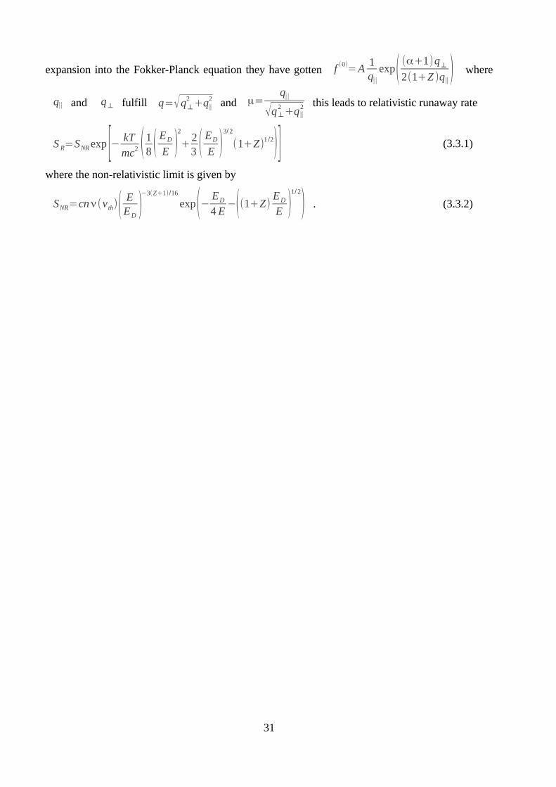
The temporal evolution of the loop voltage Uloop is shown for the shot 7398 in the Figure 2.2.
19
plasma
magneticsurface
limiter
rc
rL
R
rci
dS dγ
drift surface

Fig.2.2 Temporal evolution of the loop voltage, electric field and toroidal magnetic field during the shot #7398
The plasma is formed, when the Uloop abruptly falls, i.e at the time about 7ms. When a runaway electron has arisen at the beginning of the discharhe, the temporal evolution of its radial position is depicted in the Figure 2.3.
Fig. 2.3 Runaway electron was born at time 7.8ms. Radial position starts to increase at about 14ms. The black lines are the minor radius of the vacuum vessel of the GOLEM tokamak and limiter. The radius of the poloidal limiter is 0.085 m.
20

2.6 Dynamics and momentum space
The dynamics of a relativistic electron in a tokamak plasma is described using the test particle equations for parallel and total momentum [34] [11]
d p∣∣
d t= eE∣∣⏟
tor.el. field
−ne e4 me ln λ
4π ϵ02 γ(Zeff +γ)
p∣∣
p3
⏟collisions
− FS
p∣∣
p⏟synchrotron
(2.6.1)
d pd t
=eE∣∣
p∣∣
p−
ne e4 me ln λ
4 πϵ02
γ2
p2−FS (2.6.2)
The first term in the equations (2.6.1) and (2.6.2) is the acceleration due the toroidal electric field, and the second term includes the effect of the collisions with the plasma particles. The effects of the synchrotron radiation losses are described by means of a decelerating force
FS=23
r e m c2( vc )
3
γ4( 1
R02 +
sin4θ
rg2 )
where sin θ= p⊥ / p is the pitch angle, rg= p⊥ /eB0 is the electron gyro-radius, and re=e2
/4 πϵ0 m c2 is the classical electron radius.
Equation (2.6.1) describes evolution of a parallel momentum and (2.6.2) is equation of an energy. The system can determine whether the electron is going to be runaway or not.
Dreicer [13] solved the problem without the equation of energy. He had only 1D model and assigned the critical velocity too high. There is pointed in the Figure 2.4 as vDeicer.
If both equations (2.6.1) and (2.6.2), we get phase space with two separatrices. (see 2.4) First, let neglect the synchrotron radiation losses and define γ=1. This approach has been done in [11]. It is sufficiently when we want determine whether electron is going to or not run away. The critical velocity has been determined more precisely. Electrons situated initially under separatrice Sr will never run away. They are going to converge along Sa to origin. Electrons situated initially above Sr
lie aim asymptotically outward along Sa and therefore runaway. The saddle point VS is point of equilibrium.
When the synchrotron radiation losses are included and γ is not fixed, there has been found other stable point where the equilibrium occurs.[34] The runaway electrons are not continuously accelerated by the toroidal electric field but they reach a maximum energy when the power radiated by the electron equals the energy gain in the electric field. There is limit on the energy that the runaway electrons can reach.
21

Fig.2.4 Phase-space plot of equations (2.6.1) and (2.6.2) when FS=0 and γ=1; Sa and Sr are separatrices, VS is saddle point; α=2+Zeff, ε= E/Ec.
[12]
As a consequence of the synchrotron radiation losses, there exist some limit energy. The electron has velocity less or equal to the limit energy, never bigger. The Figure 2.5 describes this phenomenon. The green line neglect the radiation losses. The limit γS →∞ we get E/ER→1, so that for E/ER1 there is no singular point in momentum space and no runaway electrons are generated. When the radiation losses are taken into account (blue line), a local minimum exists. The minimum divides the γ into two intervals. For γ from 1 to the minimum, the line determines the critical energy. For γ from the minimum to the infinity, the line determines the limiting energy. The relation between the normalized electric field E/ER and limiting γ S is:
EER
=γS
2
γS2−1
(1+F gy
(γS2−1)
3/ 2
γSsin2
θS+F gc
(γS2−1)
5 /2
γS)
where
Fgy=2ϵ0 B0
2
3ne me ln λ and Fgc=F gy( me c
e B0 R0)
2
.
22

Fig.2.5 The normalized electric field E/ER versus γ S. Blue lined, taking into account the radiation losses; green lined, neglecting the power radiated by the electron. Electron in electric field E has velocity which lies in the area under the line.
Now, there is question whether this limit is important for tokamaks. I have calculated the limits for parameters important. The following Figures 2.6 and 2.7 show that with an increasing electron temperature the normalized electric field and the limiting γ S fall, with an increasing electron density the normalized electric field and the limiting γ S increase. The limiting γ S is around 150 in both tokamaks (see Fig. 2.8). It corresponds with 76 MeV. This limit is not important for our purpose. The electrons do not reach the energy because they hit the limiting structures before.
Fig.2.6 The normalized electric field E/ER versus the electron density in constant temperature. The left figure corresponds with COMPASS tokamak. The red line – 1000eV, the blue line – 500eV, the green line – 200eV. The right figure corresponds with GOLEM tokamak. The red line – 100eV, the blue line – 50eV, the green line – 20eV.
23

Fig.2.7 The limiting γ S versus the electron temperature for the constant electron density. The red line – 1019m-3, the blue line – 5*1018m-3, the green line – 2*1018m-3.
Fig.2.8 The γ S as function electron density and electron temperature. The temperature falls linearly. From 1000eV to 100eV at the left figure (COMPASS) and from 100eV to 10eV at the right figure (GOLEM).
2.7 Particle orbits - When is particle trapped or passing?
The particle starting at R1 with a pitch angle η1=v1⊥ /v1 at a field strength B1 and being reflected at a field strength Bmax, where
1−2v2
B1
=v2
Bmax
.
We may assume B (R)∝1/ R . So, Bmax=R1 B1
2R 0−R1.
The total fraction of trapped particle on a certain flux surface is
f trapped=√ 2rR0+r
.
The trapped particles have not the runaway velocity. In the paper [10], there is described some interesting case. The electron is trapped and ware pinch force cause its motion to the core. In the center, the particle became passing and start to runaway.
24

3 Terms in bounce averaged kinetic equation The derivation if the collision operator is in the following text. The derivation has been originally in [15]. There is a different form of the collision operator in almost each paper. That is why I compared the usual form used in [14] with one derived in 4.1. The runaway rate is also discussed in this chapter.
3.1 The collision operator
The fact that velocity of a plasma particle changes only gradually makes it possible to describe collisions by the Fokker-Planck operator.[15]
Let us consider the one-dimension distribution function f(x, v, t). If we let F(v ,Δ v) be the probability that the velocity of a particle changes from v to v+Δ v as a result of collisions in the time Δ t , the distribution function obeys
f (v , t+Δ t )=∫ f (v−Δ v ,Δ v )dΔ v .
The relation means: if a particle had the velocity v−Δ v at the time t, then the probability of it having the velocity v at the slightly later time t+Δ t is equal to F(v−Δ v ,Δ v ) . The density of particles with this history is thus f (v−Δ v , t) F(v−Δ v ,Δ v ) . Summing over all Δ v gives the total density of particles with velocity v at time t+Δ t .
In a plasma most Coulomb collisions cause only a small change in the velocity of a particle. The probability F(v−Δ v ,Δ v ) to be highly peaked around Δ v=0 in the second argument if
Δ t is small. It is therefore appropriate to treat Δ v as a small quantity and to expand f (v−Δ v , t) and F(v−Δ v ,Δ v ) in the first argument,
f (v , t+Δ t )=∫ [ f (v , t)F (v ,Δv )−Δv∂ f (v , t)F (v ,Δv )
∂ v+
(Δ v )2
2∂
2 f (v ,t )F (v ,Δ v )
∂ v2 ]d Δ v .
There is valid for all v
∫F (v , Δ v )d Δ v=1 ,
because the sum of all probabilities of velocity changes is unity. Using the notation
⟨Δ v ⟩=∫F (v ,Δv )Δ vd Δ v
⟨(Δ v )2⟩=∫F (v ,Δv )(Δ v )
2d Δ v .
The rate of change in the distribution function due to collisions is
C( f )=∂ f (v , t)
∂ t collisions
=limΔ t →0
f (v , t+Δ t)−f (v , t)Δ t
=−∂∂ v ( ⟨Δv ⟩
Δ tf )+ ∂
2
∂ v2 ( ⟨(Δ v )2⟩
2Δ tf )−... .
This is the Fokker-Planck collision operator in one velocity dimension. The first term contains the average in v, and the second term describes diffuse spreading in velocity space. The collision operator in three dimensions is
C( f )=−∇v⋅j , (3.1.1)
where jk =⟨Δ vk ⟩
Δ t− ∂
∂ v l
⟨Δ vk Δv l⟩
2Δ tf .
The angle α (see Fig. 3.1) between particle a and particle b is
25

α=ea eb
2πϵ rma v a2 ,
where r is the impact parameter.
Fig 3.1. Collision dynamics in the rest frame of particle b
Consider the two particles like only one with reduced mass m*=ma mb/(ma+mb) . The deflection angle of the relative velocity vector u= ˙r is equal to
α*=ea eb
2π ϵ0r m*u2
in the collision. Let us introduce an orthogonal coordinate system (x , y , z) , where x is the direction of va . The change of the relative velocity, caused by is then
Δux=u (cosα*−1) ,
Δu y=u sin α* cos ϕ ,
Δuz=u sin α* sin ϕ .
The changes of velocity of the particle a and their approximations for small angle α* are then
Δ vx=mb(cos α*−1)
ma+mb
u≈−(1+ma
mb)( eaeb
2π ϵ0ma)
21
2r2u3 (3.1.2)
Δ v y=mb sin α* cosϕ
ma+mb
u=eaeb
2π ϵ0ma
cos ϕ
ur
Δ vz=mbsin α*sin ϕ
ma+mb
u=ea eb
2π ϵ0 ma
sin ϕ
ur.
The number of collisions between a given particle a and particles of species b taking place in time Δ t with impact parameters between r and r +dr, and taking angles between ϕ and ϕ+d ϕ
is
Δ dϕ r d r∫ f b( v ' )ud3 v ' , (3.1.3)
26
-e
Ze
α
Φ
r

where dσ=r d r dϕ is the area spanned by d r and d ϕ , and u d t is the distance that particle a travels relative to particle b in time d t . By multiplying equations (3.1.2) with number of collisions (3.1.3) and integrating over r and ϕ , it follows that the average changes in the velocity vector of particle a as a result of collisions with particles b are
⟨Δ v x ⟩ab
Δ t=
−Lab
4π (1+ma
mb)∫ 1
u2 f b( v ' )d3 v ' ,
⟨Δ v y ⟩ab
Δ t=
⟨Δ v z⟩ab
Δ t=0 ,
where the logaritmic factor is
Lab=( ea eb
ma ϵ0)
2
ln Λ .
The values ⟨Δ vk ⟩ and ⟨Δ vk v l⟩ that we need for collision operator (3.1.1). These results are expressed in a coordinate systém aligned with the velocity vector of one of the colliding particles. In an arbitrary coordinate systém with unit vectors ek we have
⟨Δ vk ⟩ab
Δ t=
⟨ Ek⋅x Δ v x⟩ab
Δ t=
−Lab
4π (1+ma
mb)∫
uk
u3 f b( v ' )d3 v '
⟨Δ vk Δ v l⟩ab
Δ t=
⟨ ek⋅( y Δ v y+ z Δ vz) e l⋅( y Δ v y+ z Δ vz)⟩ab
Δ t=⟨(ek⋅y )(e l⋅y)(Δ v y)
2+(ek⋅z )( el⋅z)(Δ v z) ⟩
ab='
'=⟨(ek⋅e l−(ek⋅x)( el⋅x ))(Δv y)
2⟩
ab
Δ t=
⟨(δkl−uk ul
u2 )(Δv y)2⟩
ab
Δ t=
Lab
4 π∫U kl f b( v ' )d3 v '
The collision operator in Rosenbluth potentials
φb( v )=−14 π
∫1u
f b( v ')d3 v '
ψb(v )=−18π
∫uf b( v ')d3 v '
is
Cab( f a , f b)=Lab ∂∂ vk
( ma
mb
∂φ
∂ vk
f a−∂
2ψ
∂ vk ∂ v l
∂ f a
∂ v l) .
We use notation
A kab
=−⟨Δv k ⟩
ab
Δ t=(1+
ma
mb)Lab ∂ ϕ
∂ vk
Dkab
=⟨Δ vk Δv l⟩
ab
2Δ t=−Lab ∂
2ψb
∂ vk ∂ v l
.
The expression −ma Akab is force felt by a particle of species a by collisions with particles of
species b. The expression Dklab is diffusion tensor in velocity space. The Fokker-Planck collision
operator is then
27

Cab( f a , f b)=∂
∂ vk [ A kab f a+
∂∂ v l
(Dklab f a)] .
Lets consider the case of collisions between an arbitrary species a and a Maxwellian species b, where
f b(v )=nb( mb
2π kT b)
3 /2
e−
mb v2
2kTb .
Since f b is an isotropic distribution, its Rosenbluth potentials depend on the magnitude of vand not on its direction. Then
∂φb
∂ vk
=vk
vφ ' b
∂2ψb
∂v k ∂ v l
=∂
2 v∂v k ∂ v l
ψ ' b+vk v l
v2 ψb ' '=W kl ψb '+vk v l
v2 ψb ' '
where W kl=(v2δkl−vk v l)/v
3 , and a prime denotes a derivative with respect to v. If we use Lorentz operator
O( f e)=12 [ 1
sin θ∂
∂ θ (sin θ∂ f e
∂ θ )+ 1sin2
θ
∂2 f e
∂ φ2 ] (3.1.4)
we get
∂∂v k
(W kl
∂ f a
∂ v l)= 2
v3 O( f a)
and the collision operator has the form
Cab( f a , f b)=−2Lab
v3ψb ' O( f a)+
Lab
v2∂
∂v [v3( ma
mb
φ
vf a−
ψb ' 'v
∂ f a
∂ v )] .
We consider an orthogonal coordinate system where the first coordinate is aligned with the velocity vector. The first coordinate is parallel to the direction of motion. For isotropic distribution function we can write
Akab
=v (νs
ab
00
) D klab
=v2
2 (ν∣∣
ab 0 0
0 νDab 0
0 0 νDab) ,
where are introduced the three basic collision frequencies
νsab
(v)=−⟨Δ v∣∣⟩
ab
Δ t=Lab(1+
ma
mb) φ ' b(v)
v
νDab
(v)=⟨(Δ v⊥ /v )
2⟩
ab
2Δ t=−
2Lab
v3 ψ ' b(v)
ν∣∣ab
(v)=⟨(Δ v⊥ /v )
2⟩
ab
Δ t=−2Lab ψb ' ' (v )
v2 .
The slowing-down frequency νsab describes the rate at which a particle of species a is decelerated
28

by collisions with particles of species b. The deflection frequency νDab determines how quickly
the direction of the velocity vector changes, and ν∣∣ab is the parallel velocity diffusion frequency.
The collision operator has with the frequencies the form
Cab( f a , f b)=νDabO( f a)+
1
v2∂
∂ v [v3( ma
ma+mb
νsab f a+
12
ν∣∣
ab v∂ f a
∂ v )] .
This form appears with some variations in classical papers, e.g. [21] . Papers, which are concerned with generation of secondary runaway electrons [14] , use the relativistic collision operator
Cab( f a)=(mac )
3
τab [ ma
mb p2∂
∂ p(γ
2 f a)+γ
p3 O(f a)] , (3.1.5)
where γ=√1+p2
ma2 c2 and τab is the electron slowing down time defined in chapter 1.3. The
first term in the expression (3.1.4) describes friction, which causes the fast particle to slow down. This term is small if the fast particle is much lighter than the target particle. The second term describes pitch-angle scattering. The faster particle the harder to change its direction.
3.2 Collision operator in a comparison with the other paper
I have compared the collisional operator with the collisional operator in the paper [14 expression 5]. The collisional operator from the paper has a form
C=1τ [ 1
p '2∂
∂ p '(1+ p ') f +
(1+Z )
2√(1+ p '2)
p '3∂
∂ ξ(1−ξ2)
∂ f∂ ξ ] (3.2.1)
where p' is a normalized momentum p'=γvc
,
τ=4π ϵ0
2 me2 c3
ne e4 ln λis collisional time for relativistic electrons, Z is effective ion charge,
ξ=cosθ= p∣∣/ p is the cosine of pitch-angle.
Because p' is a normalized momentum, the relativistic gamma can be written γ=√(1+ p '2) .
The equation (3.1.5) do not depend on effective ion charge, but depend on the particle mass. There is almost the same. Consider only electron-electron collision, the masses ma and mb are the same and Z+1 = 2. If there is electron-ion collision, the mass in the denominator is bigger and Z increases with the charge. The rates change by the same sense.
The first therm of (3.2.1) is the same as first term in (3.1.5) without mass ratio. There is the slowing-down operator. We get the second term from (3.1.5) and from first term of (3.1.4). The second term from (3.1.4) is not included in the collisional operator (3.2.1). It means that is neglected radiation into perpendicular direction in the paper [14] .
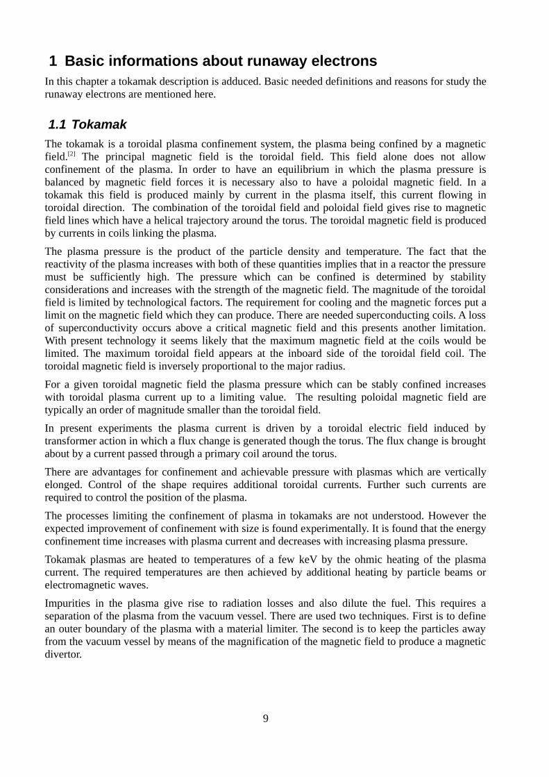
3.3 Runaway rate
The runaway rate S is source term (1.3.3) in Fokker-Planck equation. [6]
∂nr
∂ t=S
29

where nr is density of runaway electrons. Several authors have considered the problem of determining the number of runaways when [16]
E≪ ED . The earliest attempt was by Dreicer who divided velocity space into a collisional region, where the distribution function was almost spherically symmetric and a runaway region outside the spherical surface v=vc , which he considered to be empty as a result of rapid depletion by the electric field. The Fokker-Planck equation for the electrons was solved numerically as an initial-value problem following the application of the electric field to a Maxwellian plasma. The decay rate of f represented the diffusion of particles into the runaway region.
Gurevich realized that at higher velocities near v=vc distribution function f would depart from
Maxwellian and acquire a directional character concentrated near η=v∣∣
v=1 . [16] He analyzed the
region v≤vc for η∼1 as an expansion in (1−η) , so f =exp 0v1−1v 1−
22v . This form was substituted into Fokker-Planck
equation. The solution was valid for v~v th and a runaway rate is [17]
SG=2
√π nν ( EED
)1 /2
exp[− ED
4 E−( 2 ED
E )1 /2
] .
The solution for f shows a singular behavior for v →vc , the solution is only valid in a region v≤vc and Gurevich does not considered the region v≫vc .
Lebedev rectified some Gurevitch's deficiencies and his runaway rate is
SL=0.36nν(v th)( EED
)−1/ 4
exp[ −ED
4 E−( 2ED
E )1/ 2
] .
The most consistent and sophisticated treatment of this problem has been given by Kruskal and Bernstein who found it necessary to consider five distinct regions of velocity space. Connor and Hastie devoted to Kruskal's and Bernstein's work in the paper [16]. They used parameters
q=p
mcwhich is a normalized momentum and ϵ=
kTmc
which is normalized energy. First
region is q2<ϵ1/ 2 and they expanded the distribution function f in powers of ϵ :
f =f (0)+ϵ f (1) .
Second region is in range q2≈ϵ1/ 2 Because the Maxwellian exp( q2
2ϵ ) possesses no series
expansion in powers of ϵ1/ 2 they considered F=ln f and the expansion is F=ϵ
−1/2 F(0)+F (1 )
+ϵ1/ 2 F(2) .
In third region q2≈1 , the approximation expansion for F has the form
F=ϵ−1 F(0)
+ϵ−1 /2 F (1 )
+F(2) .
For α=Emc2
4π e3 n ln λ≤1 the third region extends to infinity and no runaway region exists.
Returning to the runaway case α>1 they considered the singularity q=qc in forth region where qc is a momentum when the electron is moving with a critical velocity. The most important is fifth region where q>qc . The expansion is f =f (0)
+ϵ f (1) after substituting
30
expansion into the Fokker-Planck equation they have gotten f (0)= A
1q∣∣
exp( (α+1)q⊥
2(1+Z )q∣∣) where
q∣∣ and q⊥ fulfill q=√q⊥2
+q∣∣
2 and μ=q∣∣
√q⊥2
+q∣∣2 this leads to relativistic runaway rate
S R=SNR exp [− kTmc2 ( 1
8 ( ED
E )2
+23 ( ED
E )3/ 2
(1+Z)1 /2)] (3.3.1)
where the non-relativistic limit is given by
SNR=cnν(v th)( EED
)−3(Z+1)/16
exp(− ED
4 E−((1+Z)
ED
E )1/ 2
) . (3.3.2)
31

4 Radiation losses Conditions for consideration of radiation is included at first. Than the way from Abraham-Lorentz equation to effect of radiation is composed in this chapter. I have compared three similar works about the radiation losses. At the end of the chapter is added an angle dependence of the radiation losses.
4.1 Conditions for consideration of radiation
To estimate whether the radioactive losses are or are not important, we use energy considerations. [18] If an external force field causes a particle of charge e to have to have an acceleration of typical magnitude ˙v for a period of time T. The energy radiated is of the order of
Erad≈PT
where P is Lorentz force
P=μ0 e2 v2
6π c3
which is described bellow (4.4.2). If the energy lost in the radiation is negligible compared to the relevant energy E0 of the problem, we can expect that radiative effects will be unimportant. But if
Erad≥E0 , the effects of the radiation reaction will be appropriable. The criterion for the regime where radiative effects are unimportant can thus be expressed by
Erad≪E0 . (4.1.1)
There are two different situations, one is when force is applied for finite interval T, and one where the particle and undergoes continual acceleration, e.g., in quasiperiodic motion at some characteristic frequency ω0 . For the particle at rest initially a typical energy is its kinetic energy after the period of acceleration. Thus
E0≈m(v T )2 .
The condition (4.1.1) then become
T ≫μ0 e2
6π mc3
Let define characteristic time
τch=μ0 e2
6π mc3
For time T long compared to τch radiative effects are unimportant. Only when the force is applied so suddenly and for a short time T ≈τch will the radiative effects modify the motion appreciably. The characteristic time is approximately 10-24s. This is the time taken for light to travel 10-15m.
If motion of the charged particle is quasi-periodic with a typical amplitude d and characteristic frequency ω0 , the mechanical energy of motion can be identified with the relevant energy
E0≈mω02d2 . The accelerations are v≈ω0
2 d , and the time interval is T≈1/ω0 . The criterion (4.1.1) is
ω0 τch≪1 .
32

The time ω0−1 is approximate to the mechanical motion time. If the relevant mechanical time
interval is long compared to the characteristic time τch , radiative reaction effects on the motion will be unimportant.
4.2 From Abraham-Lorentz equation to effect of radiation reaction
The velocity vector of a beam electron parallel to the magnetic field need only be scattered to acquire a Larmor rotation that can lead to substantial synchrotron radiation. [14] Since the radiation from radiation particle is emitted in a cone centered around its velocity vector, the reaction force is mainly in the direction parallel to the magnetic field althout it is the perpendicular motion that causes the radiation. I would like to describe the derivation of relativstic Abraham-Lorentz reaction force. [20] The relativistic version of motion including radiation resistance is
mc2 duμ
ds=K (4.2.1)
where uμ=γ(ct , v) is 4-vector, and radiation-reaction 4-force is given by
K=e2
6π ϵ0
d2uμ
ds2 −Ruμ
cwhere
R=−ce2
6π ϵ0
duν
dsduν
ds=
e2γ
6
6π ϵ0 c3 [ ˙v2
−( v× ˙v)
2
c2 ]≥0
is the invariant rate of energy of an accelerated charge. The space components of equation (4.2.1) get the expression which is in the paper [14]
K=e2
γ2
6π ϵ0 c3 [ ¨v+3γ
2
c2 ( v⋅˙v ) ˙v+γ
2
c2 ( v⋅¨v+3 γ
2
c2 ( v⋅˙v )2) v ]where v is the electron velocity vector and =1−v /c 2−1/ 2 is the relativistic mass factor. The time average ⟨ ...⟩ of the radiated power from an accelerated electron for which v v=0 thus becomes
−⟨ K⋅v ⟩=e2
γ4
6π ϵ0 c3∣˙v∣
2.
The energy of the particle is Ε=γme c2=me c2√1+ p '2 where p'=γ v /c is normalized
momentum, and momentum loss can be calculated from the relation Ε=K⋅v=me c2 p ' p ' / γ ,
⟨ p ' ⟩=⟨γΕ
me c2 p '⟩=
−q2γ
5
6π ϵ0me c5
⟨∣˙v∣2⟩
p' .
Let R represents the location of the gyro-center and the gyro-motion. When ≪ R the average rate of change of momentum becomes
⟨dp 'dt
⟩rad
=−√1+ p '−2
τr ( p '⊥2
+ρ0
2
R2p '∣∣
4) (4.3.2)
where τr=6π ϵ0(me c)3/e4 B2 is the radiation time scale, and 0=me c /eB . We observe that
p'∣∣=v v∣∣ p ' /c2 , and by defining the pitch-angle variable ξ≡ p '∣∣/ p ' .
An average rate of change thus becomes
33

⟨d ξdt
⟩rad
=1
γ2 p '
√1+ p '−2
τr ( p '⊥2
+ρ0
2
R2p '∣∣
4) .
The radiation reaction term is
⟨dpdt
⟩rad
∂ p∂ p
+⟨ξ
dt⟩
rad
∂ f∂ ξ
≃−1τr ( p ⊥
2+
ρ02
R2pvert
4 ) ∂ f∂ pvert
.
4.3 Comparison of [14] with [11]
I would like to compare synchrotron radiation drag force in papers [14], [10], [11].
The synchrotron radiation drag force from [14] is the expression (4.3.2). I have composed the expression
⟨dp 'dt
⟩rad
=−√1+ p '−2
τr ( p '⊥2
+ρ0
2
R2p '∣∣
4)= γ
p'
e4 B2
6π ϵ0(me c )3 ( p '⊥
2+
me2 c2
e2 B2
1
R2p '∣∣
4)='
'=γ
p'
e2 p '∣∣4
6πϵ0 me c ( 1R2 +
e2 B2 p '⊥2
me2 c2 p '∣∣
4 )= 1v
e2γ
4 v∣∣4
6π ϵ0 m0 c4 ( 1R2 +
e2 B2 p '⊥2
me2 c2 p'∣∣
4 ). (4.3.1)
The expressions in [10] and [11] are the same
FS=23
r e m c2( vc )
3
γ4( 1
R02 +
sin4θ
rg2 )
where sin θ= p⊥ / p is the pitch angle, rg= p⊥ /eB0 is the electron gyro-radius, and re=e2
/4 πϵ0 m c2 is the classical electron radius. This force has been discused in 2.6.
FS=e2
6π ϵ0( v
c )3
γ4( 1
R2+
e2 B2 p⊥2
p4 ) . (4.3.2)
Remember that p' is the normalized motion. Expressions (4.3.1) and (4.3.2) are equal when v=v∣∣ . There is simplification in [14].
The purpose of the paper [10] are numerical simulations. There is bremsstrahlung friction force included. This force is not in [14] and [11].
4.4 Angle dependence
The radiation is not isotropic and the angle dependence is quite complicated in the relativistic case.
4.4.1 Synchrotron radiation
The electromagnetic radiation emitted when charged particles are accelerated radially (a⊥ v ) is called synchrotron radiation.[21][17] When high-energy particles are in rapid motion, including electrons forced to travel in a curved path by a magnetic field, synchrotron radiation is produced. Electrons are accelerated into the X-ray range.
I am going to derive the total power radiation. I am starting with Leinard-Weichert potentials for a
34

pointed charge.
ϕ=1
4 πϵ0
q
(1−n⋅β)∣r− r p(t r)∣ret A=
μ0
4π
q v
(1−n⋅β)∣r− r p(t r)∣ret
where β=vc
and r p(t p) is a location of particle in the retarded time t r=t−∣r−r p∣
c. The
next step is calculation of an electric field. With the aid of relations
∂ t r
∂ t=1−
1c
∂ R∂ t
,∂ R∂ t
=∂ t r
∂ tn⋅v
∂∂ t
[ F ]ret=[ 1
1−β⋅n ]ret
[ F ]ret , ∇ [F ]ret=[ ∇ F]ret−[ nc (1−β⋅n) ]
ret
[ F ]ret
we have
∂ A∂ t
=[ 11−β⋅n ]
ret
q
4 πϵ0 c2∂
∂ t r [ β c
∣r−r p∣(1−β⋅n) ]∇ ϕ=
q4 π ϵ0 [ β− n
∣r −r p∣2(1−β⋅n)
2 +n
c(1−β⋅n)( cβ2+
˙β⋅n−c β⋅n
∣r −r p∣2(1−β⋅n)
2 )]ret
.
The electric field has a form
E=−∂ A
∂ t−∇ ϕ=
q4πϵ0 ( (1−β
2)( n−β)
∣r −r p∣2(1−β⋅n)
3 +1c
n×((n−β)× ˙β)
∣r −r p∣(1−β⋅n))ret
. (4.4.1)
The first term depends on 1/∣r−r p∣2 and fall very quickly. That is why, the first term can be
neglected. The second term is a radial part of electric field. An angle θ is the angle between a direction of a motion of the particle and direction of watching in the folowing expressions.Because
∣n×(n×β)∣=∣˙β∣sin θ and n⋅β=βcosθ , a radial part of the electric field has a form
Erad=q
4 πϵ0
1c
1∣r− r p∣
∣˙β∣sin θ
(1−β cosθ)3
.
An energy flux is defined S=E×B/μ0=E× n×E /(μ0c ) . We neglect first term, so E=E rad
and
S=1
(4π ϵ0)
q2
4π c1
∣r−r p∣2
β2 sin2
θ
(1−β cosθ)6 .
The power per a spherical surface is
dP=S d A=S R2sin θ dθd φ=S R2 d Ω .
The division of energy is in the time t (time of the observer)
dPdΩ
=d
dΩ ( dWdt )= S∣r −r p∣
2=
q2
4 πϵ0
14π c
β2 sin2 θ
(1−β cosθ)6 .
Full energy of the radiation is
35

P=dWdt
=∫∣r−r p∣2 S dω=
2π
4 π ϵ0
q2
4 π cβ
2∫ sin2θ
(1−β cosθ)6 d θ=
12π ϵ0
2q2 v6 c3 (1+
15
β2) .
In non-relativistic case is Larmor formula
P=1
2π ϵ0
2 q2 v2
6c3 . (4.4.2)
The share of radiation in retarded time
The power (4.4.2) is calculated in the observer time t. We want calculate the power in the retarded time tr. A difference is similar as this case: A moving gun is shoting. A frequency of shuting is not the same as a frequency of projectiles impact into target.
Pr=dWdt r
=dWdt
dtdt r
=P(1−β⋅n)
dPr
dΩ=
ddΩ ( dW
dt r )= 14 π ϵ0
q2
4π cβ
2 sin2θ
(1−β cosθ)5 . (4.4.3)
For β≪1 , the expression bracket in the denominator can be neglected. The accelerated particle emits a radiation according blue line in the Figure 4.1. As β →1 , the angular distribution is tipped forward. If we differentiate the expression (4.4.3) according θ , we get the angle with highest emission θmax .
θmax=cos−1[ 13β
(√1+15β2−1)] →
12 γ
where the last form is the limiting value for β →1 . In the Figure 4.1, the green line is the angular emission when β=0.5 .
Fig 4.1 The arrow is the direction of a particle velocity. The blue curve is the emission in different angles when the particle is non-relativistic. The largest emission is perpendicular to the direction of the particle velocity. The green curve is the emission when β=0.5 . The angle between a maximum emission and the direction of velocity is 38.2°.
4.4.2 Bremsstrahlung
Particles passing throught matter are scattered and lose energy by collisions. The radiation emitted during atomic collisions is called bremsstrahlung. For nonrelativistic particles, the loss of the energy by radiation is negligible. Compared with the collisional energy loss, but for unrelativistic particles radiation can be dominant mode of energy loss.
36

The energy flux dP through areal element d f =n R2 dΩ is
d P=S⋅d f =√ ϵμ E2 R2 dΩ (4.4.4)
where Ω is unit area. Let √ ϵμ E2 R2
=K2(t) . We use Fourier transformation and expression
(4.4.4). We find
K (ω)=ϵ0
√2πq∫
−∞
∞
ei ω t [ n×[(n−β)× ˙β ](1−β⋅n)
3 ]ret
d t .
If K (t) is real, K (−ω)=K*(ω) . The intensity of radiation emitted by a particle of charge q
during the collision can be expressed as
d2 Idωd Ω
=q2 ϵ2
π [∫−∞
∞
e i ω(t−n⋅r (t)/ c) n×[(n−β)×˙β]
(1−β⋅n)2 d t ]
2
=q2 ϵ2
π [∫dd t ( n×( n×β)
1−n⋅β )ei ω (t −n⋅r (t)/ c) d t ]2
where n and r are from the Figure 4.2
Fig.4.2 Vectors in space.
A particle's velocity is initially c β . Time of collision is the time during which significant acceleration occurs. The details of the collision will depend on the details of the collision, but its form at low frequencies depends only on the initial and final velocities. The spectrum of radiation with polarization ϵ is
limω → 0d2 IdωdΩ
=q2 ϵ2
π [ ϵ⋅( β '
1−n⋅β '−
β
1− n⋅β )]2
.
For relativistic motion in which the charge in velocity Δβ is small, the previous equation can be approximated to lowest order in Δβ as
limω → 0d2 Idω dΩ
=q2 ϵ2
π [ ϵ⋅( Δβ+ n×(β×Δβ)
(1− n⋅β)2 )]
2
.
For simplicity, we consider a small deflection so that Δβ is approximately perpendicular to the incident direction and lies in x-y plateau making an angle ϕ with x axis. The observation direction n is chosen in the x-z plane, making an angle θ with incident beam. We will average
37
n
R(t')
X
r(t')
observer
origin
electron

over ϕ . It lead to the expressions
limω → 0d2 IdωdΩ
=q2 ϵ2
2π∣Δβ∣2 (β−cosθ)
2
(1−β cosθ)4
limω → 0d2 Idω dΩ
=q2 ϵ2
2π∣Δβ∣
2 1(1−β cosθ)
2 .
The polarization
P(θ)=d I⊥−d I∣∣
d I⊥+d I∣∣
for β=0.5 is in the Figure 4.3 Maximum value is at cosθ=β .
Fig.4.3 The bremsstrahlung radiation into different angles when β=0.5 . Velocity is noted v and n is direction of maximum radiation.
Influence of synchrotron and bremmstrahlung radiation increase sharply when β →1 .
38

5 Some Analytical Estimates In this chapter are calculations and graphs which use the theory described above. I have determined the number of the runaway electron, dependence of runaway electrons on the plasma density. There is compared the influence of a collisional force, a synchrotron radiation drag force and a bremsstrahlung friction force. For comparison with subchapter 2.6, there is time of electron holding calculated different way. I have also studied HXR emission during the shot.
5.1 Number of runaway electrons
I have calculated thermalised runaway rate and number of runaway electrons in the tokamak.
Fig.5.1 Parameters used to calculate the number of runaway electrons in the COMPASS and GOLEM
The critical electric field is the electric field in which are conditions to the thermal electrons run away. The critical electric field is the lowest in the core of tokamak. That is why electrons become runaway electrons in the core more easily than on the edge of tokamak. The radial dependence of the critical electric field is in Figure 5.2.
39

The Fig.5.2 Critical electric field in GOLEM and COMPASS tokamak as function of radial position.
A normalised runaway rate is λ=S/ νne . The S has been discused in the chapter 3.3, ne is an electron density and ν is a collision frequency. At the Figure 5.3, there is a comparison of the relativistic Kruskal-Bernsein normalised runaway rate, the Lebedev normalised runaway rate, the CQL3D normalised runaway rate. The runaway rate increases on the entire edge. It is probable caused by the different gradient of the electron temperature and the electron density on the edge.
Fig.5.3 Comparison of the relativistic Kruskal-Bernsein normalized runaway rate, the Lebedev normalized runaway rate, the CQL3D normalized runaway rate.
We have calculated the number of runaway electrons in both tokamaks. We considered the tokamak as cylinder which is 2π R long and the radius is equal to the minor radius. We have divided the cylinder into 10 hollow cylinders in the case of COMPASS tokamak and 6 hollow cylinders in the case of GOLEM tokamak. The cylinders have the centers in the axis of the origin cylinder. In each coat is the constant electron temperature and the electron density. There are only the primary runaway electrons in my calculation because any secondary electrons are in the both tokamaks. Electric field is constant 1V. The runaway rate defined in 3.4 is a source term Fokker-Planck equation. I have used the relativistic Kruskal-Bernstein runaway rate. I have supposed that the shot is 200ms long in the case of COMPASS tokamak and 10ms long in the case of GOLEM tokamak. The number of runaway electrons is in the Table 5.5 and the dependence of density and number of runaway electrons on radial position is in the Figures 5.4 and
40

5.5.
Tab.5.5 The number of runaway electrons in the COMPASS tokamak and GOLEM tokamak COMPASS (200ms) GOLEM (10ms)
Number of runaways 5e+13 3e+7
Number of all electrons 6e+17 1e+17
Fig.5.4 The density of generated runaway electrons in a radial position dependence, left -COMPASS, right - GOLEM
Fig.5.5 The number of generated runaway electrons in a radial position dependence. The number of runaway electrons generated in the core is smaller because the volume is smaller. Left -COMPASS, right - GOLEM
I have calculated the rate of runaway electrons and of all electrons in real shot #2662 in COMPASS tokamak. I have used the Thomson scattering measurement. The electron temperature and the electron density has been measured 7 times during the shot. The Figure 5.6 each line is the rate of runaway electrons, i.e. the number of runaway electrons over the number of all electrons, of runaway originated between two measurements. The runaway rate is the highest between 982 – 1015ms, then the runaway rate decreases. The time of the measurements is at the Figure 5.7.
41

Fig.5.6 Each line is the rate of runaway electrons originated between two measurements. There is a radial position at the x-axis. The runaway rate is the highest between 982 – 1015ms, then the runaway rate decreases.
Fig.5.7 The Thomson scattering measurements and the course of plasma current in dependence on time.
5.2 Dependence of the runaway rate on a plasma density
I have calculated rate of runaway generation according the expressions (3.3.1) and (3.3.2) for GOLEM tokamak relevant parameters. Therefore, we estimate the plasma density from the pressure of the working gas (H2) before the discharge. We use Loschmidt constant [21]
n0=p0
k B T0 . The chamber pressure p is changing typically from 5 mPa to 25mPa at the room temperature.
42

A corresponding density of hydrogen molecules n is between 1*1018m-3 and 6*1018m-3. Assuming that fully ionized plasma is generated, the plasma density is doubled, i.e. 2*1018m-3 and 12*1018m-3. Let us assume also a homogenous distribution of the plasma density and the electron temperature inside the tokamak vessel. The figure 5.8 shows that the runaway rate increase with the increasing temperature. The decrease of the runaway rate with increasing density corresponds with experiment (chapter 7).The dependence of the runaway rate on density when temperature is 50eV for different Zeff is in the Figure 5.9. There is displayed the area where the parameters correspond to GOLEM tokamak. We have verify experimentally (Fig. 7.10). The true dependence is also in a plasma which is not clear. So, a measurement has sense in the GOLEM tokamak.
Fig.5.8 There is runaway rate in dependence on density when Zeff = 4 for different temperatures, 20, 40, 60, 80 and 100 eV
Fig.5.9 Dependence runaway rate on density when temperature is 100eV for different Zeff. The area in a rectangle corresponds to conditions in GOLEM tokamak.
5.3 Comparision of influence of collisional slowing, synchrotron and bremsstrahlung drag
In this chapter, there is described the influence of forces on the electron. The electron motion is influenced by an electric field, a collision drug and radiation losses. The radiation losses can be divided into a bremsstrahlung and a synchrotron radiation (which is further subdivided into a gyromotion and the motion of a guiding center).
43

The relations used for the influenced forces are:
the electric field force [2]
Fe=eE∣∣ ,
the collisional drag
Fcoll=ne e4 ln λ
4π ϵ02
Zeff+γ
p∣∣
2γ
2 ,
the synchrotron radiation drag force caused by the guiding center motion [11]
Fgc=23
re me c2( √ γ2−1
γ )3
γ4 1
R02
,
the synchrotron radiation drag force caused by the gyromotion
Fgyro=23
re me c2( √γ2−1
γ )3
γ4 p⊥
2 e2 B2
p4 ,
and the bremsstrahlung friction force
FB=4
137ne(Zeff−1)me c2
γ r e2( ln(2 γ)+
13 ) ,
where re is the classical electron radius re=e2
4π ϵ0 me c2 , B is the toroidal magnetic field.
The collisional drag has a major influence, when the momentum is small. With an increasing momentum, the cross section is smaller. If the collisional drag is less than electric field (region above critical velocity), the electron is continually accelerated unless the radiation losses are not considered. The influence of radiation losses increase with an increasing electron momentum. When the synchrotron radiation force curve crosses the electric field force curve the equilibrium occurs. The electron momentum can not exceed the equilibrium point. There is equilibrium limit discussed in subchapter 2.6.
The synchrotron radiation drag force caused by the gyromotion is dominant if the electron motion is small. The influence of the synchrotron radiation drag caused by the guiding center motion is small compared to gyromotion drag but at high energies increases with the increasing momentum. The bremsstrahlung friction force increases with the increasing momentum continually. The bremsstrahlung friction force has not major influence.
The Figure 5.10 demonstrates the phenomenon. There are forces which act to an electron in the electric field. The red line is an electric field force. I suppose, the electric field is constant. The black curve is the collisional force. The equilibrium occurs. The other contributions are negligible when the momentum is small. The radiation losses increase with increasing an electron momentum. Whereas the the guiding-center motion force is the smallest when the momentum is small, it tops the the electric force when the electron velocity is almost equal to speed of light. It is the second equilibrium discused in the subchapter 2.6. The electron velocity will never equal to speed of light.
44

Fig.5.10 Forces which acts to particle in a tokamak. red line – electric field force, black curve – collisional force, magenta curve – guiding-center motion force, green curve – gyromotion force, blue curve – bremsstrahlung force.
I have compared the energy limit for tokamaks GOLEM and COMPASS. The GOLEM tokamak has energy limit lower and synchrotron radiation greater than the COMPASS tokamak because the GOLEM major radius is smaller than the COMPASS one. However this limit lies in energy range around 70 MeV what is rarely reached because of the electron usually hit the tokamak's limiting structures (limiter, plasma facing material) before the energy is achieved. It is shown at the Figure 5.11.
Fig.5.11 Comparison of the GOLEM tokamak and the COMPASS tokamak energy limit. The intersection between the red line and the blue curve is the energy limit of the GOLEM tokamak and the intersection between the red line and the green curve is the energy limit of the COMPASS tokamak.
5.4 Outward drift velocity
An equation of the outward drift velocity of the runaway electron circulating orbit is derived in [10]
45
p_parallel / mc
Fo
rce
[N]

vdr=Δ xΔ t
=qs(Ee+Eeff)
B(5.4.1)
where qs is a safety factor, B is the toroidal field, Ee is electric field and Eeff is an effective electric field caused by synchrotron radiation drag force and bremsstrahlung friction force. The previous sections entitle us neglect the effective electric field. The electron leaves the plasma before it get the high energy where the effective electric field have to be included.
To calculate the time from the runaway electron origin to the hitting of tokamak's limiting structures. Equation (5.4.1) resp. (2.2.1) can be simplified under assumption Eeff << E giving equation
Δ xΔ t
=qs Ee
B
In the following table, there is the time of flight and the placed parameters. I have compared GOLEM, COMPASS, JET and ITER in the Table 5.6. The result for GOLEM corresponds with the chapter 2.5.
Tab.5.6 The comparison of time between runaway origin and the leaving of the plasma
r[m] qs B[T] t[ms]
GOLEM 0.1 3 0.2 ~10
COMPASS 0.18 3 1.2 ~100
JET 1.25 2.5 3.45 ~1
ITER 2 2.5 5.3 >1
5.5 HXR emission
I have studied the emission in more detail. There is at the Figure 5.10. There has been emitted electrons between 960 ms and 970 ms. The electrons have been hold very good and they have left the plasma when their energy has been high and start phase is not to see or there has been a lot of low-energy photons. The different situation is from 970ms to 995ms. I have thought that new runaway electrons born in time about 970ms. So I calculated the energy of electron which a velocity is equal to zero at the time and the electron is accelerated by electric field.
I measure electric field E=1V/m. I have deduced that the electron should have energy about 6MeV. It does not agree with real data. Hence I have supposed that electron is accelerated since 985ms. The energy should be about 1.5MeV at the 990ms. It corresponds with the measured signal. The electron energy increases during saturated phase. Unfortunately, there is out of the detector measuring range. The electron get energy 2π R U loop during one toroidal circle. There is 14eV. The electron with energy 1.5MeV has run 105 times around the torus. I have used for determining the velocity of the particle
γmdv∣∣
d t=eE .
46
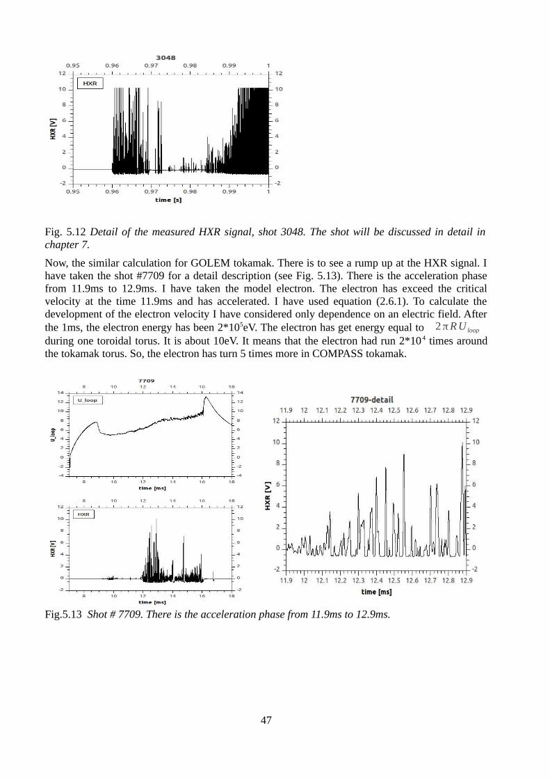
Fig. 5.12 Detail of the measured HXR signal, shot 3048. The shot will be discussed in detail in chapter 7.
Now, the similar calculation for GOLEM tokamak. There is to see a rump up at the HXR signal. I have taken the shot #7709 for a detail description (see Fig. 5.13). There is the acceleration phase from 11.9ms to 12.9ms. I have taken the model electron. The electron has exceed the critical velocity at the time 11.9ms and has accelerated. I have used equation (2.6.1). To calculate the development of the electron velocity I have considered only dependence on an electric field. After the 1ms, the electron energy has been 2*105eV. The electron has get energy equal to 2π R U loop
during one toroidal torus. It is about 10eV. It means that the electron had run 2*10 4 times around the tokamak torus. So, the electron has turn 5 times more in COMPASS tokamak.
Fig.5.13 Shot # 7709. There is the acceleration phase from 11.9ms to 12.9ms.
47

6 Numerical Codes used in Runaway electron physicsThere is description of a few codes. The codes solve the motion of runaway electrons in the tokamak.
6.1 Particle tracking codes
ASCOT (Accelerated Simulation of Charged Particle Orbits in a Tokamak) is a guiding-center orbit following code for studies of charged particles behavior in tokamaks. [23] ASCOT has been applied to study of relativistic runaway electrons and low hybrid or ion-cyclotron heating to orbit loss studies and simulations of charge diagnostic in the presence of magnetic field ripple.
In the presence of static electromagnetic fields, the relativistic guiding center motion of a collisionless particle is described by the equation of motion (2.2.1). The contributions from the grad-B and curvature drifts can be neglected in the limit rL/ L≪1 where rL is gyration radius and L is characteristic length of magnetic field variation. ASCOT uses the hybrid integration method where (2.2.1) is integrated with a fourth order Runge-Kutta algorithm. The particle location is assessed by three approximate constants of motion (2.4.1), (2.4.2), (2.4.3).
There is used Euler-Heun integration scheme for assessment an energy ϵ at time ti +1=ti+Δ t . Because the magnetic momentum μ is conserved, the perpendicular velocity at t=ti +1 is obtained by equation (2.4.3). The constant of motion Pφ can be calculated analytically.
The changes in the velocity components due to the collisions are always evaluated at the beginning of each time step at t=ti , and the invariants ϵ ,μ , Pφ are correspondingly modified. The effect of the collisions on the test particle parameters are modified by Monte Carlo collision operators based on the binomial distribution and derived from the Fokker-Planck equation. The bounce time
τB is the time need for the particle to complete one revolution or one bounce in the poloidal plane. The time step is τB/25 . ASCOT uses an analytical magnetic field model. It includes realistic features such as the Grad-Shafranov displacement of the magnetic axis, synchrotron radiation drag, plasma elongation and D-shape.
Another example of frequently used code in fusion community is ORBIT code. It uses guiding center equations as well but represented in straight field line coordinates ψ,θ , ξ . Hamiltonian guiding-center particle motion including use of numerical equilibrium and field perturbations for analyzing test particle transport. ORBIT code apply Monte Carlo method. There is implemented a fourth order Runge-Kutta integration routine.
6.2 Bounce averaged kinetic equation
The dynamics of runway electrons in a tokamak is described by a kinetic equation for the electron distribution function f coupled to Maxwell’s equations for the electric field E . [22] The full electron dynamics is, however, not required for simulating a disruption. For this purpose it is sufficient to determine the evolution of the electron distribution function on time scales short enough to resolve its behavior during a thermal quench, but much longer than the typical bounce time of an electron. As a consequence, the 6D Fokker–Planck equation can be reduced to 3D by bounce-averaging. For simplicity we consider a tokamak with concentric circular flux surfaces, and describe each particle by the three phase space variables I =( p ' , λ ,r ) , where r is the minor radius of the flux surface
48

on which the particle resides; p'=mv
m0 c is the normalized relativistic momentum where v is the
velocity, m = γm0 the relativistic mass and m0 the rest mass, and λ=p '⊥
2
p '2 b(θ), where p'⊥ is
the component of the normalized momentum perpendicular to the magnetic field and
b θ=Bθ
Bmax. Here θ is the poloidal angle, and Bmaxr is the maximum magnetic field in the
flux surface of radius r. Note that λ is defined so that particles that are trapped in the magnetic well on the outboard side of the flux surface have λ>1 while circulating particles have λ<1. The bounce-averaged relativistic Fokker–Planck equation can then formally be written as
∂ f∂ t
=⟨ LE f ⟩⟨C f ⟩⟨ L synch f ⟩⟨ L s.t. f ⟩⟨ S ⟩⟨ l B⟩
where ⟨ ...⟩ is a first momentum over a zero momentum and LE is an operator representing the parallel electric field, C(f ) is the Fokker–Planck collision operator, Lsynch represents losses due to synchrotron radiation, L s.t. is an operator representing radial transport, S is a source term of fast secondary-generated runaways, and lB is a loss term of bulk electrons such that the integral of SlB over phase space is zero, i.e. it ensures particle conservation.The evolution of the electric field is governed by Maxwell’s equations.
6.3 Focker Plank solver
I am going to describe codes CQL3D and ARENA which solve Fokker-Planck equation.
The overall aim for CQL3D is to create a general facility for the accurate calculation of heating and current drive in tokamaks. [22] CQL3D is a multi-species, 2D in velocity space, 1D in noncircular plasma radial cooordinate, fully relativistic, bounce-averaged, collisional/quasilinear Fokker-Planck equation solver. 2D in velocity space mean parallel and perpendicular velocity or a scalar energy and the pitch angle. This simplification can be used because the mean pitch angle is equal 0 and v∣∣≪v⊥ . 3D in space can be reduced because symmetry – axisymmetry and symmetry around center of cross section.The distributions are taken to be toroidally symmetric and independent of azimuthal angle about the ambient magnetic field. Radial drifts are neglected but the radial transport is included. The radial transport include diffusion and pinch terms. With the bounce-average, account is taken of variations as a function of (non-circular) radial coordinate, poloidal angle, and two momentum-space directions. A kinetic bootstrap current calculation is included. The code runs on each flux surface.Although the focus of the code has been on electrons, it is a multispecies code, i.e., it can treat electron and multiple ion distributions simultaneously. The steady state distributions and the radial rf absorption profile are obtained by iteration between the Guassian elimination solution of the Fokker-Planck equation for the steady state on each flux surface, and the rf energy transport equation integrated along a ray.
There is achieved the evolution of the electric field in a self-consistent way in ARENA code. [33]It is feasible when we need model the generation of runaway electrons in tokamak distributions. No complete simulation has been carried out the runway electron generation during a disruption. When simulating the current dynamics during a disruption, it is sufficient to calculate the evolution of the electron distribution function on time scales much longer than the bounce time (the time it takes for a particle to complete an orbit in the poloidal plane). In this case the 6D kinetic equation
49

is reduced to a 3D Fokker-Planck equation by bounce-averaging. In this code, the relativistic electron kinetic equation is solved by the Monte Carlo method, supplemented with weighting scheme to enhance the weighting scheme to enhance the accuracy of the simulated fast-electron dynamics. The main limitation of the method is the slow convergence of the solution with number of particles, leading to noisy simulations unless a large number of test particles are used. The weighting scheme is introduced to alleviate this problem. Finite elements are employed to solve Maxwell's equations governing the electric field, and this solution is coupled to the Monte Carlo solution of the kinetic equation in order to maintain numerical stability.The bounce-averaged relativistic Fokker-Planck equation is applied. There is used the following equation for the evolution of the electric field:
∇×(∇×E)=μ0∂∂ t
(σ E+ jr) .
The displacement current is neglected and the plasma current has two parts. The first part is the thermal current. The plasma conductivity is signed σ . The second is the current carried by runaway electrons in the high-energy tail of the distribution function
jr=−∫ e v (f −f b)d3 v .
6.4 Coupling of Particle tracking codes to MHD codes
NIMROD code [25] solves 3D MHD equations in global geometry. Unlike particle tracking codes, particles are in this code as liquid and the problem of huge number of particles is reduced. It get time development of these quantities:
mn∂ v∂ t
= j×B−∇ p ,
E+ v×B=η j ,
∂n∂ t
+∇⋅(n v)=0 ,
p= p(n)
The code include also curvature and grad-B drift, acceleration by electric field, and slowing due to collisions, bremmstrahlung, and synchrotron radiation. Avalanche terms are not included, the population of runaway electrons is fixed based in the initial conditions. Studies of the runaway electron avalanche are planned using NIMROD output in conjuction with CQL3D. The NIMROD code have found a sudden loss of the thermal quench. There have been studied an energy developing of a seed of electrons during the thermal quench. There have been found out that a low elongation case retains good flux surfaces longer relative to thermal quench timing. It may be related to greater separation of saturation made energies.
Like NIMROD code, the JOREK code study runaway electrons by implementation of MHD equations. The JOREK code use local coordinates of cubic Bezier grid to define vector basis for MHD equations. So, variables are projected onto vector basis. There is used fully implicit Crank-Nicholson scheme.
50

7 Experimental part
7.1 Measurement of the HXR emission on the GOLEM tokamak
7.1.1 GOLEM tokamak
The GOLEM tokamak was built in early 1960s in Moscow under a name TM-1. In 1975 the machine has been donated to the Institute of Plasma Physics, where its operation started in 1977 under the new name CASTOR (Czech Academy of Sciences TORus). A new vacuum chamber has been installed in 1985. The operation has been discontinued in 2006, when the re-installation of the COMPASS tokamak started. The tokamak CASTOR was then transported to the Faculty of Nuclear Sciences and Physical Engineering of the Czech Technical University, where it is used under a new name GOLEM for education of students. Newly, the remote operation of the GOLEM tokamak is possible. The main parameters of the GOLEM tokamak are summarized in Table 7.1.
Tab.7.1 Main parameters of the GOLEM tokamak
Major radius 0.4 m
Minor radius 0.085 m
Toroidal magnetic field < 0.5 T
Plasma current < 8 kA
Pulse length 15 ms
Plasma density 0.2 – 3*1019 m-3
Electron temperature < 200 eV
The GOLEM tokamak has a circular plasma cross section, which is defined by the poloidal limiter.
The experimental part of this thesis is devoted to measurements of the energy spectra of HXR photons. It has to be emphasized that such measurements are performed on GOLEM (and also on CASTOR) tokamaks for the first time.
7.1.2 Experimental setup
7.1.2.1 Properties of scintillator detector
We used a scintillator detector for HXR measurement on GOLEM and COMPASS. The scintillator NaI(Tl) exhibits the property of luminiscence when excited by ionizing radiation. [27] The scintillator absorb an energy of an incoming particle and re-emit the absorbed energy in the form of visible light. The NaI(Tl) detector has low density (3.67g/cm3 ). There is advisable to use for detection of low energy photons. The material is hygroscopic. So, the crystal has to be coated into an hermetic light-tight aluminum capsule. The material of the capsule is mu-metal (nickel-iron alloy). The crystal dimensions are 38 x 50.8mm. A thickness of Al envelope is 0.4 mm. The visible light from the scintillator is measured by a photomultiplier. The voltage on the photomultiplier can be change in the range of 600-1100V. The detector composed of probe head (scintillator and photomultiplier) and the preamplifier. Its picture is shown in Fig. 7.1.
51

Fig.7.1 The scintillation detector with the pre-amplifier. [26]
7.1.2.2 Calibration
The scintillator detector has been absolutely calibrated before each measurement by cesium and cobalt radiators.
Radioactive decays of the two radiators are:137
55Cs → 13756Ba + e- + νe
6027Co → 60
28Ni + e- + νe
Both of them are beta minus radiators. The decay diagram of the 137 Cs isotope is at the figure 7.2.
Fig.7.2 Decay diagram of the 137 Cs isotope.
The result of calibration is shown in figure 7.3
Fig.7.3 Time dependence of radiation cesium radiator (left) and energies of emitted photons (right).
52
137Cs
137mBa
137Ba
512keV, 94.6%
662keV1174keV5.4%
x 10
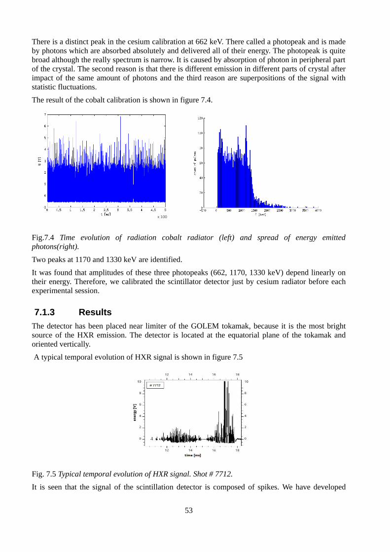
There is a distinct peak in the cesium calibration at 662 keV. There called a photopeak and is made by photons which are absorbed absolutely and delivered all of their energy. The photopeak is quite broad although the really spectrum is narrow. It is caused by absorption of photon in peripheral part of the crystal. The second reason is that there is different emission in different parts of crystal after impact of the same amount of photons and the third reason are superpositions of the signal with statistic fluctuations.
The result of the cobalt calibration is shown in figure 7.4.
Fig.7.4 Time evolution of radiation cobalt radiator (left) and spread of energy emitted photons(right).
Two peaks at 1170 and 1330 keV are identified.
It was found that amplitudes of these three photopeaks (662, 1170, 1330 keV) depend linearly on their energy. Therefore, we calibrated the scintillator detector just by cesium radiator before each experimental session.
7.1.3 Results
The detector has been placed near limiter of the GOLEM tokamak, because it is the most bright source of the HXR emission. The detector is located at the equatorial plane of the tokamak and oriented vertically.
A typical temporal evolution of HXR signal is shown in figure 7.5
Fig. 7.5 Typical temporal evolution of HXR signal. Shot # 7712.
It is seen that the signal of the scintillation detector is composed of spikes. We have developed
53
x 100

special software based on Matlab, which determines the amplitude and the width of observed peaks at the time of their appearance. It was found that the HXR signal is composed of peaks, which have different shapes. Examples of the three typical shapes are shown in figure 7.6
Fig. 7.6 Three types of registered peaks.
The left panel shows two peaks, each corresponds to a single photon. The typical width of the single peak is around 8 µs. The middle panel shows two peaks, which are partially superposed, but they can be still distinguished by the software. The right panel shows a broad peak, which corresponds detection of two or even more HXR photons in the same time. The detector signal is saturated in this case and, consequently the energy of the registered photons cannot be determined.
We have measured temporal evolution of the HXR signal in two experimental series at different discharge conditions to determine the intensity and the energy spectrum of the HXR emission:
1. The plasma current and the pressure of the working gas are kept constant, but the amplitude of the toroidal magnetic field is changed.
2. The plasma current and the toroidal magnetic field are kept constant, but the pressure of the working gas is changed.
The achieved results are described in next paragraphs in detail.
7.1.3.1 Dependence on magnetic field
The pressure of the working gas (H2) was almost the same, and it is close the requested value 10 mPa. The voltage of the condenser bank for the plasma breakdown and inductive current drive is 400 V
We have done five sets of shots with the same toroidal magnetic field under these conditions. An example of the temporal evolution of discharges with two different voltages on the condenser bank for the toroidal magnetic field, UBT is shown in fig. 7.7.
54

Fig.7.7 Temporal evolution of the loop voltage, the HXR signal and the toroidal magnetic field. Left - shot #7705, right – shot #7712
The left column of Fig. 7.7 corresponds to a typical shot from the series #7702 - #7705 with UBt
equal 600V. The drop of the loop voltage observed in 9.45ms corresponds the breakdown of the working gas and indicates start of the formation of the plasma column. The loop voltage has been 8.5V at the time. The temporal evolution of HXR photons is shown in the middle panel. The toroidal magnetic field (the bottom panel) increases from 0.09T to 0.16T during the discharge.
The right column of Fig. 7.7 corresponds to a typical shot from the series #7710 - #7713 with UBt
equal 1000V. Here, the breakdown of the loop voltage occurs at t = 8.6ms. The loop voltage is equal 7V at this time. It is interesting to note that the loop voltage drops again before the end of the shot #7712, which is a signature of a transition to regime with a better plasma confinement. This drop is accompanied with an enhanced emission of HXR photons. The toroidal magnetic field is 0.13T at the time of the breakdown and its maximum occurred at t = 17ms.
55

The differential energy spectrum of HXR photons in shots #7702 - #7705 is shown at the Figure 7.8.
Fig.7.8 Differential energy spectrum of HXR photons for shots #7702- #7705. The energy resolution is 200 keV.
In total, 1165 counts is registered in four discharges, which is in average 291 counts per one shot. The maximum seen at 5 MeV corresponds to broad peaks with the overfilled signal.
The differential energy spectrum of HXR photons of shots #7710-#7713 is shown in Figure 7.9.
Fig.7.9 The differential energy spectrum of HXR photons for shots #7410 - #7413. The energy resolution is 200 keV.
The blue bars correspond to all registered pulses. The green bars include only pulses registered apart from the time interval of the low loop voltage at the end of the discharge. In total, 1280 counts was registered (blue and green). If the HXR photons registered at the end phase are omitted, 980 photons are counted (only green bars). In average, 169 photons are counted per shot. The last maximum at 5 MeV is again connected with the broad peaks, which correspond to superposition of several photons registered in the same time.
56

Results of the scan of the HXR emission are summarized in table 7.2. I have calculated averages of counts of the sets. The counts registered during the fallings of the loop voltage are subtracted.
Tab.7.2 Dependence number of counts on the toroidal magnetic field
Btor [V] Counts per shot Short counts 15μs difference
600 293 220 73
800 267 242 25
1000 279 244 35
1200 344 301 43
1400 314 277 37
The most significant numbers are shown in the column, where counts shorter than 15μs are identified. It is evident that the number of counts depends on the toroidal magnetic field weekly. Slightly higher HXR emission is observed at the highest magnitude of toroidal magnetic field.
The distribution of HXR photons according their energies is shown in table 7.3.
Tab.7.3 Distribution of pulses according energy
Btor [V] BT – max [T] < 1MeV >1MeV
600 0.168 225 69
800 0.224 238 29
1000 0.279 256 24
1200 0.332 320 24
1400 0.386 270 44
It is seen that majority of photons have the energy under 1MeV. The most energetic photons with energies > 1 MeV are observed mainly at low toroidal magnetic field, Btor = 600 V.
Dependence on pressure of the working gas
The toroidal magnetic field constant and the voltage for primary winding of the GOLEM transformer are kept constant (U_Btor = 800V, UCD = 400 V). The initial pressure of the working gas is changed from 6 to 30 mPa on the shot-to shot basis. Most probably, higher pressure of the working gas implies higher plasma density. Unfortunately, the plasma density is not measured on GOLEM, therefore, this assumption cannot be confirmed experimentally.
Resulting dependence the HXR emission on the pressure of the filling gas (H2) is shown in figure 7.21 and Table 7.4.
57

Fig.7.10 Average number of counts registered during the discharge versus the pressure of the working gas (H2). It corresponds to results in the subchapter 5.2
Tab.7.4 There are average values. Dependence the number of counts on the pressure of the gas(H2).
Mpa counts
6 281
7 270
10 238
15 161
20 36
25 15
30 no plasma
58

Fig.7.11 Left - Differential spectra of shots #7517-7520, pressure of the filling gas has been apprpximatelly 10 mPa, Right - Differential spectra of shots #7532-7535, pressure of the filling gas has been approximatelly 25 mPa
It is evident that the intensity of the HXR emission decreases dramatically, when the pressure of the working gas increases. It can be interpreted by increasing number of slowing down collisions with increasing pressure of the working gas (plasma density).
7.1.3.2 Dependence on temperature
The temperature is not directly measured on the GOLEM tokamak. Because the generation rate for runaway electron production strongly depends on the plasma temperature, I was interested whether our HXR measurements are in qualitative agreement with the theory. To estimate approximately the electron temperature, I calculated the electron temperature from Spitzer resistivity
η=e2m1 /2
16 π ϵ02(kT e)
3/ 2 ln λ
. (7.1.1)
The plasma resistivity is deduced from the ratio of the loop voltage and plasma current.
Results of the measurements and calculation as described above are depicted in figure 7.12.
59

Fig.7.12 Temporal evolution of the HXR emission and the electron temperature in shots #7704 and #7712.
Based of this figures we can summaries our experimental observations as follows: (i) When the electron temperature had maximum the emission has been the lowest. The runaway electrons are well confined. The electron energy has grown during the phase. (ii) The higher temperature ramp-up or ramp-down the higher emission. There has been worse confinement during this non-steady phase and the magnetic surfaces have not maintained the electrons so well. (iii) When the Uloop falls rapidly at the end of the shot, the electron temperature and HXR emission increases. The confinement is better, but the changes are too abrupt to keep runaway electrons on closed orbits (see Fig. 7.12 - right). (iv) We have also verified the agreement with theory from the beginning of this subchapter by comparison of shots at the Figure 7.12, where the electron temperatures were approximately 25 eV versus 20eV. In the later case there is remarkably smaller emission the in the former case, i.e. we have confirmed that the higher temperature the higher emission.
60

Measurement of the HXR emission on the COMPASS tokamak
7.1.4 COMPASS tokamak
The COMPASS-D tokamak, originally operated by UKAEA at Culham, UK since 1992, has been reinstalled. [28] It has been moved to the Institute of Plasma Physics (IPP) AS CR in autumn 2007 and the first plasma has been achieved on 9th December 2008. The main parameters of the COMPASS tokamak already achieved are summarized in table 7.5.
Tab.7.5 Main parameters of the COMPASS tokamak currently achieved
Major radius 0.56m
Minor radius 0.18m
Plasma current 200kA
Toroidal magnetic field 1.2T
shape D, SND, ellipse
Pulse length 0,3 s
The COMPASS tokamak requires the electrical power of 75 MW for pulse duration about 2-3s. However, only 1MW power is available from the 22kV grid at the campus of IPP. So, the required power is provided by two flywheel generators.
The tokamak currently operates just with the ohmic heating. However, two Neutral Beam Injectors, already commissioned of situ, will be used for additional plasma heating by PNBI ~ 0,6 MW soon. It is expected that the ion temperature will reach the electron one. Therefore, the plasma parameters will be more relevant to large European tokamaks (ASDEX Upgrade, JET) as well as to ITER.
COMPASS is going to be upgraded with a Neutral Beam Injection (NBI) system for additional heating and current drive applications. The NBI system is already installed and consists of two injectors with beam energy 40keV and 300kW output power, delivering 600kW of total power to the plasma. Since about 20-30% of the absorbed NB power is deposited on the electrons, NBI is therefore an important electron heating mechanism.
The COMPASS tokamak is equipped by a rich set of plasma diagnostics. Among others, a sophisticated Thomson scattering system is for measuring the radial profiles of the electron density and temperature with the spatial resolution of about 10 mm and temporal resolution ~15 ms. Detailed description of the diagnostic system can be found in [34].
Currently, the HXR emission is routinely monitored by a scintillation probe, which is not absolutely calibrated. It provides the temporal evolution of the HXR emission during tokamak discharges.
This part of the diploma thesis is devoted to description of experiments with the absolutely calibrated HXR detector (the same as used for the GOLEM tokamak) to measure the energy distribution of HXR photons on COMPASS for the first time.
61

7.1.5 Experiment setup
We have used the same detector as in GOLEM tokamak. The scintillation detector is placed about 3.5m from the central solenoid of the COMPASS tokamak, close to the position of the HXR detector. The output signal is digitized by the sampling frequency 2 MHz and stored in the COMPASS database.
Fig.8.13 Left - Output signal of the scintillation detector equipped by cesium radiator for the voltage 500 V and amplification 2. Right – The corresponding energy spectrum.
7.1.6 Typical energy spectrum of HXR photons
The temporal evolution of the HXR signal as recorded by the scintillation detector is shown in Figure 7.14 for the discharge #3041.
Fig.7.14. Temporal evolution of the output signal of the scintillation detector- #3041
We typically observe a spiky signal, similar to that measured on the GOLEM tokamak.. As seen, amplitudes of some peaks are higher than 10 V. This again probably means that more than a single HXR photon is recorded simultaneously. The main feature of these high spikes is that they are noticeably broader than the "standard" ones. The distribution of the peaks according their width is shown in Fig. 7.15.
62
Time [ms] x 100

Fig.7.15. Distribution of recorded peaks according their width #3041.
We see that majority of peaks have the width between 5 – 15 µs. The wider peaks are tentatively assumed to be composed of more than one registered HXR photon.
We select the Figure 7.16 shows the energy spectrum corresponding with Figure 7.15.
Fig.7.16 Energy spectrum of HXR photons with the energy resolution 50 keV. Blue bars - all registered peaks, green bars - peaks with the width < 15 µs.
Blue bars indicate energy spectrum derived from all registered peaks, while the green bars represent spectrum of peaks with the width < 15 µs. The major difference between these two energy spectra is seen just at the highest energy 2.2 MeV, where the contribution of wider peaks is significant.
We see that maximum of the energy spectrum occurs in the energy range 50 keV. HXR photons up to 2.2 MeV are recorded.
63

The data in Figure 7.16 commemorate the plateau of distribution function of electrons in an electric field. The critical velocity is equal to 0.1221c at the core and 0.0354c at the edge. A corresponding kinetic energy is 8keV and 600eV, respectivelly. That is why we detect plateau of very fast electrons. There is corresponding with the CQL3D figures and [12]. The electron distribution function is at the Figure 7.17.
Fig.7.17 The electron distribution function in electric field in a core of COMPASS tokamak. The vector of the electric field is going from left to the right. The vertical lines borders the velocities less than the critical velocity.
As it was already mentioned, the scintillation detector is located outside the tokamak vessel. The flux of HXR photons, generated by at interaction of runaway electrons with the first wall elements or by bremsstrahlung radiation of runaway electrons, has to pass through solid state structure surrounding the plasma column, such as the vacuum vessel, flanges and magnetic coils. Consequently, the intensity of the photon flux is reduced. Let us assess this phenomenon.
Photons with an incident intensity I0, penetrating a layer of material with mass thickness x and
density ρ, emerges with intensity I given by the exponential attenuation law II 0
=exp (−(μρ ) x ) . (7.2.1)
Let us assume that the dominant material attenuating the photon flux is in our particular case iron
material of the tokamak vessel and vacuum flanged. The dependence of the coefficient (μρ ) on
the photon energy is shown for iron in figure 8.18.
64
Vc = 0.1221c
v/c
dist
ribut
ion
func
tion

Fig. 8.18. Dependence of the attenuation coefficient (μρ ) on the photon energy for iron - left.[30]
Attenuation factor, calculated from the expression (7.2.1) versus energy of photons for two values of the thickness of iron, x = 5 mm (vessel) and 15 mm (vacuum flange).
It is evident that a significant attenuation of the primary flux of HXR photons is in the range of energies (0.1 –2 MeV) and it represents a correction in the order of 1-30 % for the both cases. Figure 7.19 shows the energy spectrum of HXR photons (#3041) corrected for attenuation in iron of thickness 15 mm.
Fig. 7.19. The raw spectrum of the HXR photons in the shot #3041 (red bars) and the spectrum corrected for attenuation by tokamak structures - 15 mm of iron
7.1.6.1 Comparison with the non-calibrated HXR detector
The IPP disposes of the regular HXR scintillation detector which has different range of detection. The IPP detector has been located approximattely in the same distance from vessel but it has been in a different vertical position. Whereas the detector from FNSPE has been situated in the plane of the vessel, the IPP detector has been located over the plane. The detector has been turned on when we measured by the scintillator detector. However, the IPP detector is not calibrated. The signal of the HXR emissions of both detectors is compared in fig. 7.20 for shots #3046 and 3048.
65

Fig.7.20 Temporal evolution of shots #3046 (with a lower plasma density) and #3048 (with a higher plasma density). Panels from top to bottom: the loop voltage, line average plasma density, signal of the un-calibrated HXR detector, signal of the calibrated scintillation detector.
Let us compare at first signals of un-calibrated HXR detectors in the low- and high - density discharges. We see that the intensity of the HXR emission is extremely sensitive to plasma density, since the HXR signal in the low-density discharge (#3046) is noticeably lower then in the discharge #3048 in spite of the fact that the densities are not too much different. On the other hand, signals of the calibrated scintillation detector look quite similar. The differential spectra of the shots are in Figure 7.21.
It is necessary to note a difference between the shape of the temporal evolutions of the calibrated and un-calibrated detectors. This can be interpreted as difference in sensitivities of the both detectors. We can speculate that the calibrated scintillation detector is sensitive to less energetic photons that the un-calibrated one, because its signal appears earlier.
66

Fig.7.21 Differential spectra of shots #3046 (left) and #3048 (right).
7.1.7 Discusion
The experimental part is dedicated to the results of measurement of HXR signal at GOLEM and first results from COMPASS. There are more sources of HXR during discharge but main contribution is from electrons which hit PFC. The signal has been measured by scintillator detector from FNSPE and IPP.
The FNSPE detector has been calibrated by cesium and cobalt radiators. We have measured photons up to 5 MeV in GOLEM and up to 2.2 MeV in COMPASS.
For data processing, I have calculated the width of peaks. Based on this analysis I decided that peaks shorter than 8µs detect only one photon has been detected probably. When the peak was broader, the peak is was superposed of two or more counts. The saturated peaks has been broad up to 15µs and energy of a detected signals can not be determined. It has been caused by photons which energy is higher than 5MeV, resp. 2.2MeV and by the signal superposed from more photons.
We have measured the dependence on three parameters influencing the properties of plasma and subsequently appearance of runaway electrons. First was the voltage in the toroidal magnetic coils UBt, second the pressure of the filling gas p and the third was electron temperature Te.
– We have not find some clear dependence of HXR emission on the toroidal magnetic field. Broad peaks has been detected in a wide range in a small toroidal magnetic field. It mean probable that the huge number of electrons with a lower energy has been emitted.
– When the pressure increases, the number of detected counts decrease because a collision drug increases. It agrees with theory discussed in subchapter 5.2 (Fig. 5.9) where is shown the dependence of runaway rate on a density in constant temperature and for different Zeff.
– We have also verified that with the higher temperature there is a higher emission of runaway electrons as is predicted by equation (7.1.1) giving runaway rate. The measured dependence of runaway rate on the temperature is shown in the Figure 5.8.
Unfortunately the measurement quality was deteriorated by a few factors. Uncertainty of screening of mainly low energy HXR due to attenuation. We can not see, e.g. energy spectra in the vicinity of critical energy.
The detector has been located outside the tokamak vessel. We have also decided that low-energy
67

photons are attenuated in the materials of tokamak vessel (Fig. 7.19). When the electron has a velocity equal a critical velocity the corresponding energy is about 8keV in COMPASS tokamak. We have detected electrons with energy higher than the value. The consequence is that we measured plateau of distribution function of electron in electric field (Fig. 7.16) and we have verified the output data from CQL3D (Fig. 7.17).
68

8 ConclusionIn this diploma thesis I have summarized basics of runaway electron theory (in chapters 2-4 and chapter 6), I have computed estimates for some important physical parameters concerning runaway electrons physics (in chapter 5) and I have made measurements on GOLEM and COMPASS tokamaks (in chapter 7) as well.
The runaway electrons are electrons created in the presence of toroidal electric field by surpassing the point in velocity space where collisional drag is lower the the electric acceleration force and so a way to substantial acceleration is opened because collisional drag is decreasing function of velocity. There are more mechanism of runaway electron generation present in tokamks (primary, secondary/avalanche, gama ray excitation, hot-tail, low-hybrid waves). In my diploma thesis I have described in high detail especially primary mechanism which is the most important for small and middle size tokamaks (see chapter 1.3 and 3.3). A systematic study of runaway have begun by Dreicer (1959).[13] In 1961, Gurevich[17] have developed more accurate equations for calculation of the runaway rate and the critical electrons but he have not calculated relativistic case which aply for the case of small electric fields. The relativistic version, the most accurate and the most complex calculations have made Kruskal and Bernstein. Their work has been presented by Connor and Hastie in 1975.[16] The runaway rate is source term in Fokker-Planck equation.
Secondary mechanism caused by close collisions of a thermal electron with already existing runaway electron population are described in subchapter 1.3. The avalanche mechanism is not important for GOLEM or COMPASS tokamaks but will be in ITER because the multiplication process occurs when the lifetime of plasma in larger multiple of the time elapsed between two short-range collisions. Detailed overview of other mechanisms would go out of scope of this work.
In chapter 3, I have presented also quit properly process of collisions which was important for expressions giving rise to generation rates as mentioned above and which are also important for already existing RE dynamics (slowing down, pitch angle scattering). I have presented in a detail derivation of the runaway rate from a collision operator with Rosenbluth potentials across a collision operator with Lorentz operator for an angle dispersion. In the collision operator there are included a slowing-down frequency for parallel velocity, a parallel velocity diffusion frequency and a deflection frequency for pitch angle. . I have compared different forms of collisional operator which are found on papers.[14]
Once runaway electron created, i.e. the electron get over the critical velocity, great part of physic is based on a quite complicated motion in tokamak magnetic and electric field. For theoretical as well as practical needs it is more convenient to use guiding center equation of motion instead of the full particle motion including fast gyro-motion. Nowadays, probably most advanced guiding center equations (used also in gyrokinetic theory)[17] are discussed in detail in chapter 2. Conditions for their use are satisfied very well for RE case where the gyroradius is small compared to gradients of magnetic field and magnetic field is slowly-warying compared to gyrofrequency. In subchapter 2.3, I have shown how from this equations follows “standard” drifts which can be found in classical textbooks. The constants of motion are in subchapter 2.4. One effect following from the conservation of the constants of motion is an radial outward drift moving runaway electrons to the PFC. I have computed a runaway holding time for GOLEM tokamak and I found that this effect limits maximal energy RE can gain
Guiding-center equation of motion does describe just pure motion. Influence of collisions and radiation and the implications of this processes are described in the subchapter 2.6. The motion of the particle in dynamics and momentum-space can be described by the equation of the change of a parallel momentum (2.6.1) and by equation of the energy change (2.6.2). If radiation losses are not
69

considered there is only one equilibrium/stable point in a momentum-space.[12] This is the situation when collisional drags is equal to an electric field force. On the other hand, when the radiation losses are considered, there appears a second equilibrium/stable point.[11] This is energy limit, when the radiations losses force is equal to the electric field force, is called synchrotron limit. The electron can not get over the momentum any more at the given value of electric force.
When we study RE dynamics more precisely we have to take into account also radiation losses. This is the theme of the forth chapter. I showed the strange of particulars effects in a quite explanatory logarithmic plot (see 5.10). The energy radiated is directly proportional to Lorentz force and a time period of the motion. The radiation can be neglected when the radiated energy is much smaller than other energies which affect on the electron. The radiation losses can be divided into synchrotron radiation caused by the guiding-center motion, synchrotron radiation caused by the gyromotion and bremsstrahlung. I have compared a synchrotron radiation drag force in papers [10], [11], and [14]. I have computed that in [14] is simplified expression. A velocity is equal to a parallel velocity. The nonrelativistic accelerated particle emits a radiation perpendicular with a velocity vector. When a relativistic particle is accelerated an angle between a largest radiation and the velocity vector is less than a right angle. I have calculated by using Matlab when a electron velocity is equal 0.5c the synchrotron radiation angle is 38.2°. Influence of synchrotron and bremsstrahlung radiation increase sharply is a relativistic case.
In the chapter 5, the critical electric field, i.e. electric field in which thermal electrons can runaway, as function of a radial position is depicted in GOLEM and COMPASS tokamaks. I have compared the relativistic Kruskal-Bernstein normalized runaway rate, Lebedev normalized runaway rate and a normalizes runaway rate which is an output parameter in CQL3D code. According anticipation, the Lebedev normalized runaway rate is less accurate because it is nonrelatvistic expression. I have estimated the density and number of runaway electrons in GOLEM and COMPASS tokamak as function of a radial position. I have decided that the rate between runaway electrons and the all other electrons is about 1:105 in COMPASS tokamak. In GOLEM tokamak, the number of runaway electrons is less than in COMPASS. I have used for determination of a runaway electron density a method of deposits as well as is used in CQL3D. The density of runaway electrons is the highest in the core but an absolute number of runaway electrons is not amazingly in the core of a tokamak vessel. The number of runaway electrons generated in the core is smaller because the volume is smaller. The highest number of runaway electrons is origined in approximately one third of a minor radius. I have also calculated that runaway rate increase with the increasing electron temperature and I have graphically represented a dependence runaway electron rate on an electron density for different Zeff when temperature is constant. We verified the calculations experimentally. Consequently, the true dependence is also in a plasma which is not clear. I have computed an outward drift velocity. In comparison with an energy limit (subchapter 2.6), I have decided that a runaway electron hit PFC much earlier than it get the limit energy. An electrons do not reach the limit energy in a both tokamaks.
In the sixth chapter, numerical codes are described. Particle tracking codes are ASCOT and ORBIT. CQL3D and ARENA use a bounce-average kinetic equation. NIMROD and JOREK solves 3D MHD equations.
In the seventh chapter is an experimental part. We have measured HXR on GOLEM and COMPASS tokamaks. The scintillator detector has been used. There has been first measurements in the tokamaks. We have measured a typical time development of HXR, a width of the peaks and height of the peak which corresponds with energy. We have observed the dependence of runaway production on the toroidal magnetic field Btor, the electron density ne, the electron temperature Te, and the pressure of the filling gas p. As expected, we have detected more runaways with higher energy in COMPASS tokamak. We have verified theoretical predictions. The most detected electrons have had energy up to 5MeV. It is only small part of an energy limit (apprpximatelly
70

75MeV). We have verified a accuracy of outward drift velocity calculations. We have measured the higher emission in a higher electron temperature (Fig. 5.8). We have decided that the higher density of the filling gas the lower runaway rate. I have predicted the dependence in the Figure 5.9. When the electron has a velocity equal a critical velocity the corresponding energy is about 8keV in COMPASS tokamak. We have detected electrons with higher energy. That is why we meassured plato of distribution function of electron in electric field (Fig. 7.16) and we have verified the output data from CQL3D (Fig. 7.17).
71

9 Appendix
9.1 Lagrangian and Hamiltonian
The Lagrangian formulation allows one to use arbitrary coordinates in configuration space. [29]
[17]The Lagrangian for a set of coordinates q=(q1, q2, ..., qN) where N denotes the number of degrees of freedom, is a function of the coordinates and its derivatives. The equations of motion follow from requiring a trajectory's action
S (q j)=∫t1
t2L(q ,q , t)=0
to be stationary with respect to variations of the trajectory q (t) in configuration space. This requirement yields the Euler-Lagrangian equations
ddt L
q j − L q j
=0 (10.1.1)
for the trajectory. For charged particle motion in an electromagnetic field the Lagrangian in Cartesian coordinates for a particle of mass m and charge e is
L( x , ˙x , t)=m2
∣˙x∣2+e ˙x A( x , t)−eϕ (10.1.2)
in terms of the scalar potential ϕ and the vector potential A , which give the electromagnetic
field via E=∇ ϕ−∂ A∂ t
and B=∇×A .
We define the canonical momentum p with components
pi=∂ L∂ q i
( q , ˙q , t) .
We use Lagrange transformation to get Hamiltonian H (q , p , t)= p ˙q (q , p , t)−L( q , ˙q , t) .
In Cartesian coordinates, the Hamiltonian corresponding to a charged particle moving in an electromagnetic field is
H ( x , p , t)=1
2m∣p−e A∣
2+e ϕ( x , t) .
The equations of motion are Hamilton's equations
qi=∂ H∂ pi
, p i=−∂ H∂ qi
.
While Hamiltonian mechanics treats the coordinates and momenta on equal footing and allows for a broader class of transformations, the set of transformations is yet restricted to canonical transformations. To define these transformations, it is convenient to denote the phase-space point by the 2N-dimensional vector z=(q1, ... , qN , p1,... pN) . The transformation to another set of coordinates Z ( z , t) is canonical if there is fulfilled for Jacobian matrix
Dαβ=
∂ Zβ
∂ zα
the condition D⋅σ⋅D†=σ , where σ is the fundamental symplectic 2N×2N matrix
σ=( 0 δij
−δij 0 ) (10.1.3)
and D† denotes the transpose of D . The fundamental symplectic form (10.1.3) defines the Poisson brackets of the coordinates and the canonical momenta among themselves
{zα , zβ}=σαβ .
72

For any two functions f and g in these phase-space, the canonical Poisson bracket is a
{f , g }=∂ f∂ zα
σαβ
∂ g∂ zβ
.
Canonical transformations are defined as those for which the Poisson bracket remains an invariant form. Canonical transformation have the property of serving the form of Hamiltonian's equations. That is, for any Hamiltonian H (q , p , t ) and any canonical transformation ( p , p)→(Q , P) to new coordinates Q(q , p , t) and momenta P(q , p , t) , there exists a new variables by Hamiltonian K (q , p , t) giving the evolution of the new variables by Hamilton's equations
Qi=∂ K∂ Pi
, Pi=−∂ K∂ Qi
.
A phase-space Lagrangian should be easily transformed to an arbitrary set of phase-space coordinates. The phase-space Lagrangian for the noncanonical variables ( x , v ) is
L=( m v+e A ( x ,t ))⋅x−(eϕ+m2
∣v∣2) . (10.1.4)
We yield from the equation (10.1.1) Lorenz force on a charged particlem ˙v=e E+e ˙x×B .
(10.1.5)The guiding-center phase space consists of the guiding-center position X , essentially the center of the helix, the guiding-center parallel velocity variable u=b⋅˙X , the magnetic moment
μ=m∣w∣
2
2B( X , t),
where w=v⊥−v E is perpendicular velocity in the local frame moving with the E×B drift velocity v E , and the ignorable gyrophase ξ , which gives the location of the particle on the circle about the guiding center. As there are still six variables parametrizing phase space, there is no loss of information in making the guiding-center transformation ( x , v )→( X ,u ,μ ,ξ) . For the sake of simplicity of notation, we occasionally use the gyroaction variable J=(m /e)μ insteed of the magnetic moment μ whenever we need to refer to the action-angle coordinates (J ,ξ)associated with gyromotion.The equations of motion for these variables are given by the guiding-center Lagrangian
Lgc X ,u , ,; t =[e A X , t mu b ]⋅XJ −Hgc (10.1.6)in which the guiding-center Hamiltonian is given by
Hgc=m2
u2 B X , t eX ,t −
m2
∣v E X , t ∣2
.
The guiding-center Lagrangian comes not simply from gyrophase averaging, but from a transformation from the variables ( x , v ) to guiding-center variables ( X , u ,μ ,ξ) . We apply (10.1.1) to (10.1.5), we get again Lorenz force, unlike (10.1.5) in a guiding-center coordinates
mu b=e ( E *+ ˙X ×B*) .We can identify effective electromagnetic fields from this record:
E *=−∇ ϕ*−1c
∂ A *∂ t
B *=∇×A *
and effective electromagnetic potentials are
e ϕ*=eϕ+μ B−m2
∣vE∣2, A *= A+
me
u b .
9.2 Relativistic Lagrangian and Hamiltonian
The relativistic motion of a particle of rest mass m and charge e is described in eight-dimensional
73

phase space in terms of the space-time coordinates x=x0=ct ,x and the four-momentum p
=mu with the four-velocity defined as
u=
dx
d
where =1−v2
c2 −1 /2
is relativistic factor and dx/d = x . Minkowski space-time matrix
is gμ ν=(
−1 0 0 00 1 0 00 0 1 00 0 0 1
)so that u u=−c2 is invariant. The equation of motion for the four-momentum p is
dp
d =
ec
F u
where
Fμ ν=∂
μ A ν−∂
ν Aμ=(
0E x
c
E y
c
E z
c−E x
c0 −Bz By
−E y
cBz 0 −Bx
−E z
c−B y Bx 0
)denotes the Faraday tensor. Here the space-time contravariant derivative is
∂μ=gμ νuν=(−∂/∂ x0,
∇) and Aμ=( A0
=ϕ , A ) is the electromagnetic four-potential.There are two Hamiltonian formulations for the relativistic equations of motion for a charged particle moving in an electromagnetic field. First formulation is based on a covariant description expressed in terms of the phase-space coordinates (xμ , pμ
) . The covariant formulation treats space and time as well as momentum and energy on equal footings. The second formulation treats time and space separately and makes use of the extended phase-space coordinates ( x , p , t , w) , where the energy coordinate w is canonically conjugate to time t.If we consider covariant formulation, the covariant form is invariable, but there are some discrepancy. The covariant relativistic particle motion takes place on the surface
H c (xμ , pμ)=−mc2
/2 , hence Hc is a Lorentz scalar. Furthermore, the covariant relativistic Hamiltonian does not have a well-defined nonrelativistic limit, which can make it impractical. So, I doing focus on the noncovariant formulation. For weakly time-dependent fields, the relativistic guiding-center phase-space Lagrangian [4] is expressed in terms of extended guiding-center phase-space coordinates Za
=( X , p∣∣;μ ,ς ; w , t) as
Lrgc=[ e A+ p∣∣b ]⋅X +μ ( mce )ς−w t−H rgc
where Za=dZa
/d σ and σ represents Hamiltonian orbit parameter in extended phase-space and physical particle motion in eight-dimensional extended phase-space. The relativistic guiding-center extended Hamiltonian is
H rgc=γmc2+e ϕ( X ,t )−w
where γ=√1+(2 /mc2)μ B( X ,t )+ p∣∣
2/(mc)
2 is the guiding-center relativistic factor and the relativistic guiding-center extended Poisson bracket is
74

{F ,G }rgc=em ( ∂ F
∂ ξ∂ G∂μ
−∂ F∂μ
∂ G∂ ξ )+ B *
B∣∣*⋅(∇ * F
∂ G∂ p∣∣
−∇ *G∂ F∂ p∣∣
)− be B∣∣*
⋅∇ *F×∇ *G+( ∂ F∂w
∂G∂ t
−∂ F∂ t
∂ G∂w )
where the effective gradient operator ∇* is
∇*=∇−e∂ A *∂ t
∂∂w
,
the effective magnetic field is
B *=∇× A *=B+( p∣∣
e )∇×b
and
B∣∣*=b⋅B *=B+( p∣∣
e ) b⋅∇×b .
The effective electric field is
E *=−∇ ϕ*−1c
∂ A *∂ t
=E−1e (mc2 ∇ γ− p∣∣
∂ b∂ t ) .
The relativistic guiding-center Hamiltonian equations are expressed asdZa
d σ={Z a, H rgc }rgc .
75

10 References[1] http://www.guardian.co.uk/environment/2011/aug/23/fusion-power-is-it-getting-closer[2] WESSON, J., at.al. Tokamaks, Clarendon Press, Oxford, 2004, 3rd edition[3] ITER Physics Basic, Nuclear Fusion, 1999, vol.39, no.12, 2251-2389[4] Progress in ITER Physics Basic, Nuclear Fusion, 2007, S128-S202[5] SOKOLOV, Yu. A. “Multiplication” of accelerated electrons in a tokamak, JETP Lett., 1979, vol.29, no. 4[6] FEHÉR T. at.al., Simulation of runaway electron generation during plasma shutdown by impurity injection in ITER. Plasma Phys.Control. Fusion, 2011, vol.53, 17pp, 035014[7] CARY, J. - BRIZARD, A. Hamiltonian theory of guiding-center motion. Reviews of modern physics, April-June 2009, vol.81, no.2, 693-738[8] CHEN F.F. Introduction to Plasma Physics, London, Plenum, 1984, 2nd edition [9] KNOEPFEL, H. - SPONG, D.A. Runaway electrons in toroidal discharges. Nuclear fusion, 1979, vol.19, 785-829[10] GUAN, X., QIN, H., Phase-space Dynamics of Runaway Electrons In Tokamaks, Princeton Plasma Physics Laboratory, 2010[11] MARTIN-SOLIS, J.R. at.al. Momentum–space structure of relativistic runaway electrons , Physics of Plasmas, 1998, vol.5, no.6, 2370-2377[12] FUCHS, V., Velocity space structure of runaway electrons, Phys. Fluids 29, 1986, 2931-2936[13] DREICER, H., Electron and Runaway in a Fully Ionized Gas, Physical Review, 1959, vol.117, no.2, 329-342[14] ANDERSSON, A. Damping of relativistic electron beams by synchrotron radiation. Phys. of plasmas, December 2001, vol.8, no.12, 5221-5229[15] HELANDER, P. - SIGMAR, D.J. Collisional Transport in Magnetized Plasmas, Cambridge[16] CONNOR, J.W. - HASTIE, R.J., Relativistic limitations on runaway electrons. Nuclear fusion, 1975, vol.15, 415 - 424[17] GUREVICH, A.V. On the theory of runaway electrons. Soviet physics, 1961, vol.12, no. 5, 904-912[18] JACKSON, J. D., Classical Electrodynamics, Wiley, 1975, 2nd edition[20] McDONALD, K.T., Limits on the Applicability of Classical Electromagnetic Fields as Inffered from the Radiation Reaction, 1998, NJ 08544[21] http://en.wikipedia.org/wiki/Synchrotron_radiation[22] ERIKSSON, L.-G. Simulation of runaway electrons during tokamak disruptions. Computer Phys. Communications, 2003, vol.154, 175-196[23] HEIKKINEN, J.A., Monte Carlo Simulation of Runaway Electrons in a Toroidal Geometry Comput. Phys. Comm. 76, 1993, 215-230 [24] HARVEY, R.W. - McCOY, M.G., The CQL3D Fokker-Planck Code, 4th November 2005[25] IZZO, V. A., at.al. Runaway electron confinement in MHD disruption mitigation simulations, Atlanta, 2009, prezentation[26] http://www.phywe.com/461/pid/26558[27] http://astronuklfyzika.cz/DetekceSpektrometrie.htm[28] PÁNEK, R. at.al. Reinstallation of the COMPASS-D Tokamak in IPP ASCR, Czechoslovak Journal of Physics, 2006, vol.56, B125-B137 [29] GOLDSTEIN, H. – POOLE, Ch.– SAFKO, J. Classical Mechanics. Addison Wesley, 3rd
edition[30] http://physics.nist.gov/PhysRefData/XrayMassCoef/tab3.html[31] HARMS, A. A. et. al, Principles of Fusion Energy, World Scientific Publishing, 2005 [32] FRIEDBERG, J., Plasma physics and fusion energy, Cambridge, 2007[33] ANDERSSON, F. Runaway Electrons and Current Dynamics During Tokamak Disruptions,
76

presentation[34] WEINZETTL - V., at.al., Overview of the COMPASS diagnostics Fusion Engineering and Design, Vol.86. 2011, 1227-1231
77