CZCRC and FRDC Final Report Environmental Flows for ... · that a significant proportion of the...
29
CZCRC and FRDC Final Report Environmental Flows for Fisheries in Sub-tropical Estuaries Chapter 4. Climate impacts on barramundi and banana prawn fisheries of Queensland tropical east coast J. Balston Summary The commercial catch of barramundi (Lates calcarifer) and the banana prawn (Penaeus merguiensis) displays a high degree of inter-annual variation; a characteristic that many fishers believe is the result of climate variability. However, studies to examine the effects of the full range of climate variables are limited and the impact of some variables, such as evaporation, have never been considered. This chapter examined the effects of short-term (inter-annual) climate variability on the commercial catch of wild barramundi and banana prawn in Princess Charlotte Bay of north-east Queensland. A life-cycle model of each species was developed to link climate variables with the developmental stages of the species from spawning through to catch. Fisheries (catch and effort) and climate (rainfall, freshwater flow, evaporation, sea surface temperature, terrestrial temperature and indices of the SOI and MJO) data were extracted from a variety of sources and compiled for analysis. A gamma-distributed logarithm-link function model was constructed to calculate total freshwater flow for those years when flow records were incomplete. Correlation analysis was used to identify significant relationships between climate variables and catch, and forward stepwise ridge regression was used to model catch using climate variables as predictors. Warm sea surface temperatures in January – March, high rainfall in July – September and January - March, increased freshwater flow in January – March and low annual evaporation (all measures of an extensive and productive nursery habitat) were all significantly and positively correlated with barramundi catch two years later as recorded by the CFISH logbook system. These results suggest that early barramundi survival is enhanced in these conditions. Catchability of barramundi was significantly increased after high freshwater flow and rainfall from October – December in the year of catch, reinforcing the observation that mature fish in freshwater habitats are flushed into the commercial estuarine fishery. A forward stepwise ridge regression model built to predict commercial barramundi catch in Princess Charlotte Bay contained July – September rainfall, annual evaporation and January – March sea surface temperatures two years prior to catch and explained 63% of the variance in catch. The model had a cross validated predictive R 2 of 49%. A comparative analysis of data from the anthropogenically modified Fitzroy River area returned far fewer significant relationships, a result that indicated changes to habitat either affected or masked the relationship between other climate variables and barramundi catch in the area. A correlation analysis between seasonal and annual climate variables and banana prawn catch in the Princess Charlotte Bay area in the year of catch did not return any significant relationships. Other studies of rainfall and banana prawn catch gave significant correlations with catch data from beam trawlers only. Results with catch data from otter trawlers were not significant – the primary method of harvest in Princess Charlotte Bay. Results from the current chapter indicate that a significant proportion of the variability seen in commercial barramundi catch in north-east Queensland is driven by variability in climate. Evaluation of approach and methods The objective of this section was to raise the awareness of natural climate variability and its impact on freshwater flows, dependant fisheries and water allocation management through the delivery of outputs relating to the CZCRC AF project research question (ii) i.e., What are the impacts of natural climate variability upon estuarine fisheries and therefore environmental flow allocations to sustain healthy estuarine communities? An initial analysis of the variability of Chapter 4. Climate impacts on barramundi and banana prawn fisheries 63
Transcript of CZCRC and FRDC Final Report Environmental Flows for ... · that a significant proportion of the...

CZCRC and FRDC Final Report Environmental Flows for Fisheries in Sub-tropical Estuaries
Chapter 4. Climate impacts on barramundi and banana prawn fisheries of Queensland tropical east coast
J. Balston
Summary The commercial catch of barramundi (Lates calcarifer) and the banana prawn (Penaeus merguiensis) displays a high degree of inter-annual variation; a characteristic that many fishers believe is the result of climate variability. However, studies to examine the effects of the full range of climate variables are limited and the impact of some variables, such as evaporation, have never been considered. This chapter examined the effects of short-term (inter-annual) climate variability on the commercial catch of wild barramundi and banana prawn in Princess Charlotte Bay of north-east Queensland.
A life-cycle model of each species was developed to link climate variables with the developmental stages of the species from spawning through to catch. Fisheries (catch and effort) and climate (rainfall, freshwater flow, evaporation, sea surface temperature, terrestrial temperature and indices of the SOI and MJO) data were extracted from a variety of sources and compiled for analysis. A gamma-distributed logarithm-link function model was constructed to calculate total freshwater flow for those years when flow records were incomplete. Correlation analysis was used to identify significant relationships between climate variables and catch, and forward stepwise ridge regression was used to model catch using climate variables as predictors.
Warm sea surface temperatures in January – March, high rainfall in July – September and January - March, increased freshwater flow in January – March and low annual evaporation (all measures of an extensive and productive nursery habitat) were all significantly and positively correlated with barramundi catch two years later as recorded by the CFISH logbook system. These results suggest that early barramundi survival is enhanced in these conditions. Catchability of barramundi was significantly increased after high freshwater flow and rainfall from October – December in the year of catch, reinforcing the observation that mature fish in freshwater habitats are flushed into the commercial estuarine fishery. A forward stepwise ridge regression model built to predict commercial barramundi catch in Princess Charlotte Bay contained July – September rainfall, annual evaporation and January – March sea surface temperatures two years prior to catch and explained 63% of the variance in catch. The model had a cross validated predictive R2
of 49%. A comparative analysis of data from the anthropogenically modified Fitzroy River area returned far fewer significant relationships, a result that indicated changes to habitat either affected or masked the relationship between other climate variables and barramundi catch in the area.
A correlation analysis between seasonal and annual climate variables and banana prawn catch in the Princess Charlotte Bay area in the year of catch did not return any significant relationships. Other studies of rainfall and banana prawn catch gave significant correlations with catch data from beam trawlers only. Results with catch data from otter trawlers were not significant – the primary method of harvest in Princess Charlotte Bay. Results from the current chapter indicate that a significant proportion of the variability seen in commercial barramundi catch in north-east Queensland is driven by variability in climate.
Evaluation of approach and methods The objective of this section was to raise the awareness of natural climate variability and its impact on freshwater flows, dependant fisheries and water allocation management through the delivery of outputs relating to the CZCRC AF project research question (ii) i.e., What are the impacts of natural climate variability upon estuarine fisheries and therefore environmental flow allocations to sustain healthy estuarine communities? An initial analysis of the variability of
Chapter 4. Climate impacts on barramundi and banana prawn fisheries 63

CZCRC and FRDC Final Report Environmental Flows for Fisheries in Sub-tropical Estuaries
rainfall and freshwater flow was undertaken using historical data from the Australian Rainman StreamFlow 4.3 TM package (Clewett et al. 2003). Rainfall across Queensland is highly variable as seen from the historical records for each of the two areas considered in this section of the study: the Fitzroy region of central Queensland and Princess Charlotte Bay (PCB) in the far north of the state (Figure 4.1). This variability is amplified in freshwater flows which are in some cases an order of magnitude higher than recorded rainfall for the catchment (Figure 4.2). Because of this, both inter-annual and inter-decadal climate variability needs to be taken into account when analysing data from a short time series in order to contextualise the results into a historical setting. In the rainfall graph (Figure 4.1), the study period considered in this analysis is overlayed onto the historical time series.
Figure 4.1 Annual rainfall variability at Yaamba station on the Fitzroy River and Musgrave station in Princess Charlotte Bay (1900-2004)
0
500
1000
1500
2000
2500
1900
1904
1908
1912
1916
1920
1924
1928
1932
1936
1940
1944
1948
1952
1956
1960
1964
1968
1972
1976
1980
1984
1988
1992
1996
2000
2004
Year
Ann
ual r
ainf
all (
mm
)
Yaamba
Musgrave
Study period
Figure 4.2 River flows entering Princess Charlotte Bay River between 1971-1987
0.0
200000.0
400000.0
600000.0
800000.0
1000000.0
1200000.0
1400000.0
1600000.0
1800000.0
Jan
Aug MarOct
MayDec Ju
lFeb
Sep Apr NovJu
nJa
nAug
MarOct
MayDec Ju
lFeb
Sep Apr NovJu
nJa
nAug
MarOct
Years
Flow
V ol
um e
(M l)
Deighton River
East Normanby
Hahn River
Kennedy River
Laura River
Normanby River
Stewart River
West Normanby
A literature review of published papers and other reports was undertaken to determine climatic factors which might impact on each of the species studied: barramundi (Lates calcarifer) and banana prawn (Penaeus merguiensis). Based on this review, and as recommended by Vance et al.
Chapter 4. Climate impacts on barramundi and banana prawn fisheries 64
CZCRC and FRDC Final Report Environmental Flows for Fisheries in Sub-tropical Estuaries
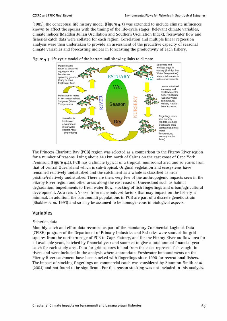
(1985), the conceptual life history model (Figure 4.3) was extended to include climate influences known to affect the species with the timing of the life-cycle stages. Relevant climate variables, climate indices (Madden Julian Oscillation and Southern Oscillation Index), freshwater flow and fisheries catch data were collated for each region. Correlation and multiple linear regression analysis were then undertaken to provide an assessment of the predictive capacity of seasonal climate variables and forecasting indices in forecasting the productivity of each fishery.
Figure 4.3 Life-cycle model of the barramundi showing links to climate
Mature males return to estuary to aggregate with females on spawning grounds (Early season freshwater flow)
Spawning and fertilized eggs in estuary (Salinity; Sea Water Temperature). Mature fish remain in saline environments.
Larvae entrained in estuary and postlarvae enter nursery habitats (Salinity; Water Temperature; Nursery Habitat Area; Access)
Fingerlings move from nursery habitats into tidal creeks and then upstream (Salinity; Water Temperature; Nursery Habitat Area )
Maturation of males in freshwater habitat 2-4 years (Water Temperature)
Juveniles in freshwater environment (Freshwater Habitat Area; Temperature)
ESTUARY
RIV
ER
Wet
Season
Dry
NU
RSE
RY
The Princess Charlotte Bay (PCB) region was selected as a comparison to the Fitzroy River region for a number of reasons. Lying about 340 km north of Cairns on the east coast of Cape York Peninsula (Figure 4.4), PCB has a climate typical of a tropical, monsoonal area and so varies from that of central Queensland which is sub-tropical. Original vegetation and ecosystems have remained relatively undisturbed and the catchment as a whole is classified as near pristine/relatively undisturbed. There are then, very few of the anthropogenic impacts seen in the Fitzroy River region and other areas along the east coast of Queensland such as habitat degradation, impediments to fresh water flow, stocking of fish fingerlings and urban/agricultural development. As a result, ‘noise’ from man-induced factors that may impact on the fishery is minimal. In addition, the barramundi populations in PCB are part of a discrete genetic strain (Shaklee et al. 1993) and so may be assumed to be homogeneous in biological aspects.
Variables
Fisheries data Monthly catch and effort data recorded as part of the mandatory Commercial Logbook Data (CFISH) program of the Department of Primary Industries and Fisheries were sourced for grid squares from the northern edge of PCB to Cape Flattery, and for the Fitzroy River outflow area for all available years, batched by financial year and summed to give a total annual financial year catch for each study area. Data for grid squares inland from the coast represent fish caught in rivers and were included in the analysis where appropriate. Freshwater impoundments on the Fitzroy River catchment have been stocked with fingerlings since 1990 for recreational fishers. The impact of stocking fingerlings on commercial catch was considered by Staunton-Smith et al. (2004) and not found to be significant. For this reason stocking was not included in this analysis.
Chapter 4. Climate impacts on barramundi and banana prawn fisheries 65

CZCRC and FRDC Final Report Environmental Flows for Fisheries in Sub-tropical Estuaries
Figure 4.4 Princess Charlotte Bay region showing river systems, estuarine and near shore habitats, adjacent coral reefs and CFISH grid squares
Rainfall For PCB splined rainfall data were sourced from the Bureau of Meteorology (BOM) spatially interpolated rainfall and climate database (SILO). A detailed explanation of how the rainfall surface was created can be found at the SILO website (http://www.bom.gov.au/silo). Total monthly rainfall for five locations in PCB corresponding to Annie River (14o 30’S; 143o 42’E), Port Stewart (14o 06’S; 143o 42’E), Normanby River (14o 24’S; 144o 12’E), Aloszville station (14o 24’S; 144o 00’E) and Lakefield (14o 57'S; 144o 12'E) were extracted from the database and used to calculate an average monthly local area rainfall data set. For the Fitzroy region, local area average total seasonal rainfall data was calculated from data extracted from Rainman StreamFlow 4.3 (Clewett et al. 2003) for stations within the coastal region of the Fitzroy River estuary (i.e. Bajool, Mt Morgan, Mt Larcom, Rockhampton, Port Alma, Langmorn, Raglan, Stanwell and Gracemere) as per Staunton-Smith et al. (2004).
Freshwater flows Monthly freshwater flow data for each region were collected from the Department of Natural Resources and Water (NRW) stream gauge website database (http://www.nrm.qld.gov.au/watershed/index.html). This included for PCB total monthly flow for all rivers in the basin with gauges (eight in total) and for the Fitzroy region the Gap station (the most downstream gauging station) minus the estimated downstream extraction. For PCB, monthly flow from each river was summed in order to calculate total monthly flow into the bay, and missing data identified. Recent years were missing for many of the gauge stations and so total basin flow for years corresponding to CFISH data was modelled using the full set of data for the period January 1971 to February 1987 as the base period (a time series of 133 consecutive months with no missing values). A gamma distributed logarithm link function model which included each month as a variable was developed (i.e. the model changes depending on the month being calculated). As the Normanby, East Normanby and Laura rivers each showed high correlations with total basin flow and have recent data, they were selected for the generation of total flow for the years with missing data in other rivers.
Chapter 4. Climate impacts on barramundi and banana prawn fisheries 66

CZCRC and FRDC Final Report Environmental Flows for Fisheries in Sub-tropical Estuaries
Temperature Maximum and minimum air temperature and evaporation were sourced from the BOM SILO database (http://www.bom.gov.au/silo) for Lakefield National Park in PCB (14o 57'S; 144o 12'E; 40 m) and for two grid points aligning with the mouth of the Fitzroy river (23 o 30’S; 150 o 48’E) and Keppel Bay (near Broadmount/Port Alma, 23° 30'S 150° 48'E) in the Fitzroy study area as representative points. Monthly and seasonal averages, and annual total temperature degree days (sum of daily temperatures) were calculated for both maximum and minimum air temperature.
Sea surface temperatures As there are no in situ recordings for sea surface temperatures in PCB or the Fitzroy River region, data were sourced via the web from the Physical Oceanography Distributed Active Archive Center (PO.DAAC), generated by the National Aeronautics and Space Administration (NASA) Jet Propulsion Laboratory at a resolution of 1oC, and is accurate to within 0.5oC (http://podaac.jpl.nasa.gov/products/product119.html). Monthly averaged data for PCB were extracted for the point 14oS; 114oE in PCB and the point 23oS; 151oE for the Fitzroy River region. Monthly and seasonal average and annual total temperature degree days were calculated for analysis.
Southern Oscillation Index (SOI) Monthly average values of Troup’s SOI (Troup 1965) were extracted from the Department of Natural Resources and Water ‘LongPaddock’ website which uses a base period from 1887 to 1989 (www.longpaddock.qld.gov.au). The index is derived from normalised Tahiti minus Darwin mean sea level pressure.
Madden Julian Oscillation (MJO) All Season Real Time Multi-Variate MJO Indices (RMM) were sourced from the Bureau of Meteorology Research Centre website (http://www.apsru.gov.au/mjo/) and include both phase (as defined by a longitudinal position of the centre of the oscillation) and the number of days in each phase. The variable used in the analysis was a count of the number of days for each phase over the northern wet season (defined here as 1 November - 30 April). This corresponds to the time of the year when the MJO has the strongest influence on the region.
Wind Mean monthly V-wind (meridional – north/south) and U-wind (zonal – east/west) data were extracted for the point 14oS; 114oE for PCB from the NCEP/NCAR Reanalysis Data: Derived Products data request web page at the NOAA Climate Diagnostics Centre (http://www.cdc.noaa.gov/cdc/data.ncep.reanalysis.derived.html#surface). Data is at sea level for a 2.5-degree latitude x 2.5-degree longitude grid. Wind data were used only for analysis with the banana prawn data and were averaged for each spawning season: March to May for the autumn spawning; August to October for the spring spawning. Annual total wind run (summed daily wind vector ms-1) was also calculated for each vector.
Selected data were checked for normality using histograms and the Shapiro-Wilks test and transformed where necessary. In order to capture the monsoonal climate cycles, the seasons were defined as per Vance et al. (1998): pre-wet (October to December); wet (January to March); early dry (April to June) and dry (July to September). This varies from the seasons defined by Robins et al. (2005), and was selected in order to capture the northern monsoon wet in one season. Annual data, where used, was for the financial year (1st July to 30th June). A summary of data sets collated for analysis is shown in Table 4.1.
Chapter 4. Climate impacts on barramundi and banana prawn fisheries 67
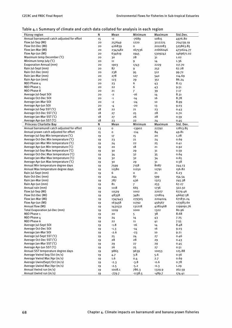
Table 4.1 Summary of climate and catch data collated for analysis in each region Fitzroy region N Mean Minimum Maximum Std.Dev. Annual barramundi catch adjusted for effort Flow Jul-Sep (Ml) Flow Oct-Dec (Ml) Flow Jan-Mar (Ml) Flow Apr-Jun (Ml) Maximum temp December (oC) Minimum temp July (oC) Evaporation Annual (mm) Rain Jul-Sept (mm) Rain Oct-Dec (mm) Rain Jan-Mar (mm) Rain Apr-Jun (mm) MJO Phase 4
15 20 20 20 20 20 20 20 20 20 20 20 20
-0 257649 426839 2347482 634619 30 11 1903 87 238 278 123 23
-7689 1220 0 167536 1945 28 9 1743 9 95 127 29 6
10815 3112225 2012083 21666046 5309242 31 14 2229 252 512 540 351 43
4976.80 704239.19 525863.85 4731624.77 1469671.02 1.02 1.36117.70 67.28 99.72 114.69 86.24 8.13
MJO Phase 5 20 22 6 43 9.51 MJO Phase 8 20 21 7 39 7.17 Average Jul-Sept SOI Average Oct-Dec SOI Average Jan-Mar SOI Average Apr-Jun SOI Average Jul-Sep SST (oC) Average Oct-Dec SST (oC) Average Jan-Mar SST (oC) Average Apr-Jun SST (oC)
20 20 20 20 18 18 18 18
-2 -1 -2 -4
22 27 27 23
-16 -14 -24 -20 21 25 26 22
14 16 10 13 23 28 28 24
8.31 8.78 8.99 9.03 0.430.700.590.45
Princess Charlotte Bay N Mean Minimum Maximum Std. Dev. Annual barramundi catch adjusted for effortAnnual prawn catch adjusted for effort Average Jul-Sep Min temperature (oC) Average Oct-Dec Min temperature (oC) Average Jan-Mar Min temperature (oC) Average Apr-Jun Min temperature (oC) Average Jul-Sep Max temperature (oC) Average Oct-Dec Max temperature (oC) Average Jan-Mar Max temperature (oC) Average Apr-Jun Max temperature (oC)
Annual Min temperature degree days Annual Max temperature degree daysRain Jul-Sept (mm)
Rain Oct-Dec (mm) Rain Jan-Mar (mm) Rain Apr-Jun (mm) Annual rain (mm) Flow Jul-Sep (Ml) Flow Oct-Dec (Ml) Flow Jan-Mar (Ml) Flow Apr-Jun (Ml) Annual flow (Ml)
Total Evaporation Jul-Dec (mm) MJO Phase 1
13 15 19 19 19 19 19 19 19 19 19 19 19 19 19 19 19 19 19 19 19 19 19 19
0 0 17 23 24 20 30 34 32 30 7599 11580 6 244 787 81 1118 11529 48358 1347443 163458 1431531 1209 20
-13902 -114 15 21 22 18 29 32 32 29 7158 11250 0 87 436 7 665 1002 3481 279305 11792 131218 1000 5
22792 84 20 24 25 21 31 35 34 31 8087 11791 21 599 1323 253 1736 22077 170824 2204024 456567 4282468 1322 38
12813.85 49.81 1.28 0.69 0.41 0.92 0.59 0.64 0.65 0.58 244.13 156.82 6.23 154.54 245.38 67.27 322.50 6779.46 46697.58 671831.24 123583.60 1199091.76 80.96 8.68
MJO Phase 4 19 24 14 43 7.25 MJO Phase 6 19 22 11 41 7.55 Average Jul-Sept SOI Average Oct-Dec SOI Average Jan-Mar SOI Average Jul-Sept SST (oC) Average Oct-Dec SST (oC) Average Jan-Mar SST (oC) Average Apr-Jun SST (oC) Annual SST temperature degree days
Average Vwind Sep/Oct (m/s) Average Vwind Mar/Apr (m/s) Average UwindSept/Oct (m/s)
Average Uwind Mar/Apr (m/s) Annual Vwind run (m/s) Annual Uwind run (m/s)
19 19 19 19 19 19 19 19 19 19 19 19 19 19
-1.8 -1.3 -2.6 25 28 29 26 9865 4.7 1.6 -2.3 -2.5
1008.1 -779.7
-16 -14 -23 24 28 27 25 9639 3.8 0.4 -3.8
-5.2 786.3 -1138.5
14 16 10 27 29 29 27 10053 5.6 2.7 -0.6
-0.3 1329.9
-489.7
8.48 9.03 9.21 0.46 0.430.45 0.51 125.88 0.56 0.69 0.78 1.29 162.59 174.41
CZCRC and FRDC Final Report Environmental Flows for Fisheries in Sub-tropical Estuaries
Chapter 4. Climate impacts on barramundi and banana prawn fisheries 68
CZCRC and FRDC Final Report Environmental Flows for Fisheries in Sub-tropical Estuaries
Fitzroy River region Expanding on the analysis of barramundi and rainfall/freshwater flow interactions, additional climate variables and climate indices which were identified in the barramundi life-cycle were selected for analysis. A correlation matrix of all relevant climate variables (for barramundi analysis lagged up to five years) and catch adjusted for effort was generated to identify significant relationships and possible collinearity between independent variables. Some of the independent variables were found to be significantly correlated with each other; however, as each describes a mechanism which affects the fishery in a different biological way (e.g. freshwater flow in the river bed versus rainfall replenishing wetland habitat separate from the river) in the earlier stages of the analysis, it was considered valid to include them. Collinearity between independent variables was compensated for through the use of forward stepwise ridge regression (FSRR) modelling (StatSoft. Inc. 2005). As not all of the variables were collineated and correlations where they did exist were weak, the ridge regression constant l (lambda) was initially set at 0.1. Three different FSRR models were built. The first used each of the climate variables which showed a significant correlation to catch in the correlation matrix, including lagged variables (Climate Variables Model). The second model incorporated each of the indices of the SOI and MJO for all lags (Climate Indices Model), and the third model used only significantly correlated climate variables lagged by two and three years (Predictive Model) so as to capture impacts on early life-cycle stages of the fish. The first two allowed for a comparison between the use of climate variables and climate indices in describing catch. The third explored the possibility of generating predictions of future catch with sufficient time for a response from fisheries managers and/or operators. Models were limited to three steps, as the use of more variables in the model risks an artificially high level of the variance being accounted for, and a corresponding decrease in forecasting skill due to the increased degrees of freedom (Shepherd et al. 1984). Residuals were checked for normality using a normal probability plot and for auto-correlation using the Durbin-Watson statistic. Adjusted coefficients of determination (R2) which take into account the degrees of freedom in the model were calculated (StatSoft. Inc. 2005).
Princess Charlotte Bay region Analysis for the PCB region followed the same methodology outlined for the Fitzroy analysis and determined the appropriateness of transferring methodologies and results spatially.
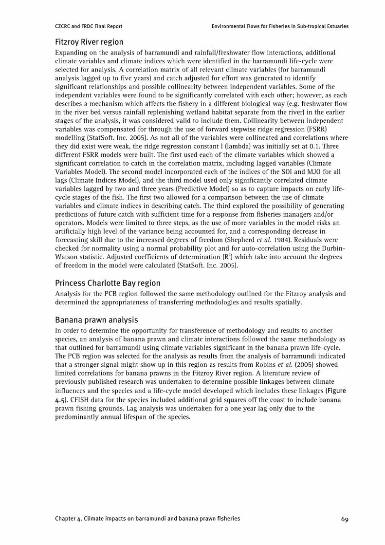
Banana prawn analysis In order to determine the opportunity for transference of methodology and results to another species, an analysis of banana prawn and climate interactions followed the same methodology as that outlined for barramundi using climate variables significant in the banana prawn life-cycle. The PCB region was selected for the analysis as results from the analysis of barramundi indicated that a stronger signal might show up in this region as results from Robins et al. (2005) showed limited correlations for banana prawns in the Fitzroy River region. A literature review of previously published research was undertaken to determine possible linkages between climate influences and the species and a life-cycle model developed which includes these linkages (Figure 4.5). CFISH data for the species included additional grid squares off the coast to include banana prawn fishing grounds. Lag analysis was undertaken for a one year lag only due to the predominantly annual lifespan of the species.
Chapter 4. Climate impacts on barramundi and banana prawn fisheries 69
SSEdeleted = 1−
Predictive R2 SST (Equation 4.1)
n ˆ )2SSEdeleted = ∑(y − dii d̂
iwhere i=1 and yi is the ith observed value and is the predicted value when
yi is not included in the analysis.
CZCRC and FRDC Final Report Environmental Flows for Fisheries in Sub-tropical Estuaries
Figure 4.5 Life-cycle model of the banana prawn showing links to climate
Spring and autumn spawning of adults offshore (Salinity;
Sea Water Temperature; Wind
Speed and Direction)
Larvae dispersed by currents to estuarine
nursery habitats (Salinity; Water
Temperature; Wind Speed and Direction)
Postlarvae in estuary / nursery habitat (Salinity;
Water Temperature)
Some individuals over-winter (Water Temperature)
Juveniles migrate to coastal flats and inshore areas with freshwater flows to mature (Freshwater flows; Rainfall; Temperature)
OFFSHORE
ESTUARY
Migration of mature prawns to the offshore fishery (Freshwater flows, rainfall)
INSHORE
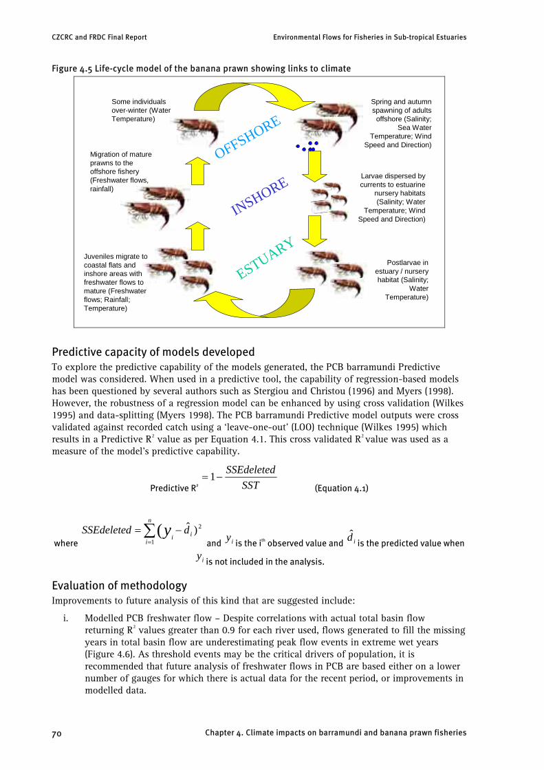
Predictive capacity of models developed To explore the predictive capability of the models generated, the PCB barramundi Predictive model was considered. When used in a predictive tool, the capability of regression-based models has been questioned by several authors such as Stergiou and Christou (1996) and Myers (1998). However, the robustness of a regression model can be enhanced by using cross validation (Wilkes 1995) and data-splitting (Myers 1998). The PCB barramundi Predictive model outputs were cross validated against recorded catch using a ‘leave-one-out’ (LOO) technique (Wilkes 1995) which results in a Predictive R2 value as per Equation 4.1. This cross validated R2 value was used as a measure of the model’s predictive capability.
Evaluation of methodology Improvements to future analysis of this kind that are suggested include:
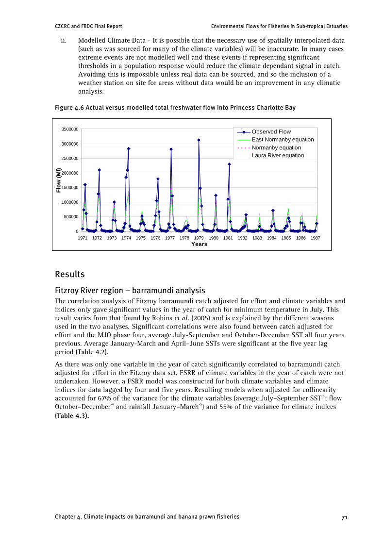
i. Modelled PCB freshwater flow – Despite correlations with actual total basin flow returning R2 values greater than 0.9 for each river used, flows generated to fill the missing years in total basin flow are underestimating peak flow events in extreme wet years (Figure 4.6). As threshold events may be the critical drivers of population, it is recommended that future analysis of freshwater flows in PCB are based either on a lower number of gauges for which there is actual data for the recent period, or improvements in modelled data.
Chapter 4. Climate impacts on barramundi and banana prawn fisheries 70
CZCRC and FRDC Final Report Environmental Flows for Fisheries in Sub-tropical Estuaries
ii. Modelled Climate Data - It is possible that the necessary use of spatially interpolated data (such as was sourced for many of the climate variables) will be inaccurate. In many cases extreme events are not modelled well and these events if representing significant thresholds in a population response would reduce the climate dependant signal in catch. Avoiding this is impossible unless real data can be sourced, and so the inclusion of a weather station on site for areas without data would be an improvement in any climatic analysis.
Figure 4.6 Actual versus modelled total freshwater flow into Princess Charlotte Bay
0
500000
1000000
1500000
2000000
2500000
3000000
3500000
1971 1972 1973 1974 1975 1976 1977 1978 1979 1980 1981 1982 1983 1984 1985 1986 1987 Years
Flow
(Ml)
Observed Flow East Normanby equation Normanby equation Laura River equation
Results
Fitzroy River region – barramundi analysis The correlation analysis of Fitzroy barramundi catch adjusted for effort and climate variables and indices only gave significant values in the year of catch for minimum temperature in July. This result varies from that found by Robins et al. (2005) and is explained by the different seasons used in the two analyses. Significant correlations were also found between catch adjusted for effort and the MJO phase four, average July-September and October-December SST all four years previous. Average January-March and April–June SSTs were significant at the five year lag period (Table 4.2).
As there was only one variable in the year of catch significantly correlated to barramundi catch adjusted for effort in the Fitzroy data set, FSRR of climate variables in the year of catch were not undertaken. However, a FSRR model was constructed for both climate variables and climate indices for data lagged by four and five years. Resulting models when adjusted for collinearity accounted for 67% of the variance for the climate variables (average July–September SST-4; flow October–December-4 and rainfall January–March-5) and 55% of the variance for climate indices (Table 4.3).
Chapter 4. Climate impacts on barramundi and banana prawn fisheries 71

CZCRC and FRDC Final Report Environmental Flows for Fisheries in Sub-tropical Estuaries
Table 4.2 Correlation coefficients (r) between the barramundi catch adjusted for effort and selected climate variables in the Fitzroy River region
Variable 0 lag 1 year lag 2 year lag 3 year lag 4 year lag 5 year lag
Maximum temp Dec (oC) 0.35 0.17 -0.51 -0.48 0.03 0.47
Minimum temp Jul (oC) -0.75* -0.19 0.20 0.14 0.31 -0.29
Evaporation Annual (mm) 0.16 0.07 -0.35 -0.31 -0.48 0.04
Rain Jul-Sept (mm) -0.46 -0.31 0.14 0.21 0.34 -0.41
Rain Oct-Dec (mm) -0.19 0.04 0.46 -0.38 0.41 0.25
Rain Jan-Mar (mm) 0.26 0.11 0.03 -0.51 0.12 -0.11
Rain Apr-Jun (mm) 0.02 0.36 -0.25 0.16 -0.27 0.04
MJO Phase 4 0.04 0.28 0.10 0.05 -0.64* -0.22
MJO Phase 5 -0.06 0.20 -0.02 0.08 0.03 0.04
MJO Phase 8 -0.03 -0.13 -0.24 -0.14 0.28 -0.27
Average Jul-Sept SOI -0.22 -0.13 0.18 0.00 0.44 -0.24
Average Oct-Dec SOI -0.31 0.07 0.46 0.19 0.38 -0.34
Average Jan-Mar SOI -0.09 0.23 0.42 -0.03 0.13 -0.46
Average Apr-Jun SOI -0.14 0.08 0.26 0.20 0.05 0.02
Average Jul-Sep SST -0.21 -0.13 -0.13 0.05 0.77* -0.37
Average Oct-Dec SST 0.11 0.26 -0.41 -0.55 0.52* 0.20
Average Jan-Mar SST 0.16 0.11 -0.21 -0.22 -0.06 0.59*
Average Apr-Jun SST 0.18 -0.11 0.12 -0.36 -0.07 0.71*
Flow Jan-Mar (Ml) 0.18 -0.13 0.17 -0.41 0.18 -0.03
Flow Apr-Jun (Ml) -0.25 0.04 -0.08 0.09 -0.07 0.23
Flow Oct-Dec (Ml) -0.17 -0.12 0.51 -0.42 0.58 0.03
Flow Jul-Sep (Ml) -0.37 0.00 0.20 -0.05 0.50 -0.07
(*P<0.05)
Table 4.3 Comparison of forward stepwise ridge regression models for the Fitzroy region CFISH barramundi catch
Climate Variables Model (adjusted R2=0.67) Intercept Average Jul-Sep SST (4 year lag) Flow Oct-Dec (4 year lag) Rain Jan-Mar (5 year lag) Climate Indices Model (adjusted R2=0.55)
Regression coefficient
-179142* 7619*
5* 1302
Standard error
44283.27* 1886.14*
2.14* 893.33
p-level
0.003* 0.003* 0.038*
0.179
Intercept MJO Phase 4 (4 year lag) Average Oct-Dec SOI (5 year lag) MJO Phase 5 (5 year lag)
19115* -6017* -366*
1818
7265.15* 1534.72* 126.02*1064.05
0.025* 0.003* 0.016*
0.118 (*P<0.05)
Residuals for the Climate Variables Model were normally distributed, independent (Durbin-Watson statistic; P<0.05) and fell within +2 standard deviations of the mean, indicating an absence of outliers. However, in the Climate Indices Model the financial year 1989/1990 was an outlier.
Princess Charlotte Bay region – barramundi analysis The correlation matrix between selected climate variables and barramundi catch adjusted for effort identified 12 significant correlations (Table 4.4). The FSRR Climate Variables Model (Table 4.5) included rain July-September–2 (two years previous); evaporation annual–2 and average October-December SOI (no lag), and explained 68% of the variance in catch adjusted for effort. The Climate Index Model explained 53% of the variance with average October-December SOI (no lag), MJO Phase 4–1 and July-September SOI-2. The Predictive Model contained rain July-
Chapter 4. Climate impacts on barramundi and banana prawn fisheries 72

CZCRC and FRDC Final Report Environmental Flows for Fisheries in Sub-tropical Estuaries
September–2, evaporation annual–2 and average January-March SST–2 and explained 63% of the variance (Table 4.4). Once again, residuals for all models were normally distributed, independent (Durbin-Watson statistic; P<0.05) and fell within + 2 standard deviations of the mean.
Table 4.4 Correlation coefficients (r) between barramundi catch adjusted for effort and selected climate variables for the Princess Charlotte Bay region
Variable 0 lag 1 year lag 2 year lag 3 year lag 4 year lag Minimum temp Jul (oC) 0.10 -0.16 -0.25 -0.62* -0.27 Maximum temp Dec (oC) -0.55 -0.25 -0.02 0.06 0.21 Rain Jul-Sept (mm) -0.01 0.02 0.77* 0.46 0.48 Rain Oct-Dec (mm) 0.56* 0.30 0.38 0.15 -0.06 Rain Jan-Mar (mm) 0.56* 0.31 0.62* 0.12 0.26 Rain Apr-Jun (mm) 0.37 0.40 -0.02 0.14 0.08 Flow Jul-Sep (Ml) 0.36 0.41 0.33 0.18 -0.34 Flow Oct-Dec (Ml) 0.71* 0.37 0.29 -0.02 -0.13 Flow Jan-Mar (Ml) 0.52 0.35 0.76* 0.36 0.43 Flow Apr-Jun (Ml) 0.33 0.33 0.13 0.27 0.08 Evaporation Annual (mm) -0.73* -0.48 -0.62* -0.34 -0.15 Average Oct-Dec SST (oC) 0.12 0.25 0.40 0.46 0.56* Average Jan-Mar SST (oC) 0.32 0.17 0.58* 0.03 0.29 MJO Phase 1 -0.55 0.00 -0.26 -0.08 0.17 MJO Phase 4 0.04 -0.39 -0.18 0.05 0.54 MJO Phase 6 0.38 0.50 0.16 0.21 -0.09 Average Jul-Sept SOI 0.47 0.12 0.29 0.13 0.06 Average Oct-Dec SOI 0.62* 0.19 0.29 0.14 0.14 Average Jan-Mar SOI 0.47 -0.18 0.10 0.19 0.37
(*P<0.05)
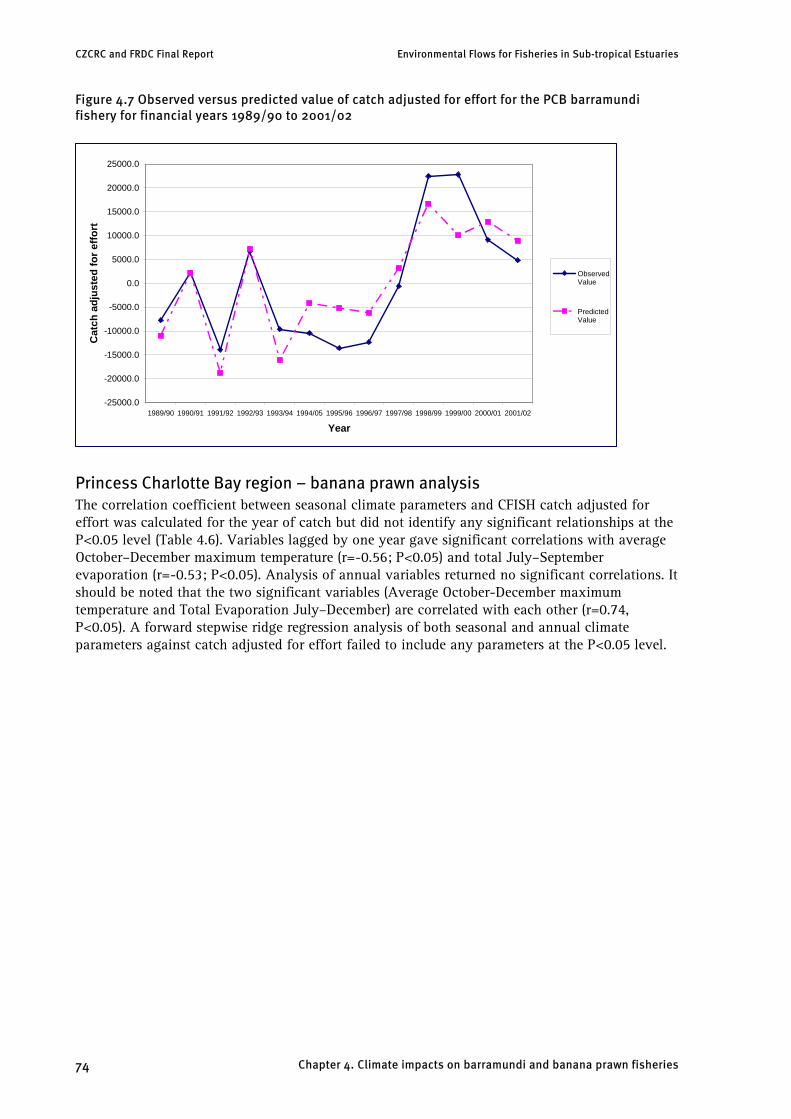
Predicted versus observed values of catch were plotted for the Predictive Model with all but four points falling within the 95% confidence limits (Figure 4.7). Cross validation of the Predictive Model returned an adjusted R2 of 0.48 compared to an R2 of 0.63 initially calculated. This shows the robustness of the model and indicates that even when used in a predictive capacity, the Predictive Model is explaining nearly half the variance in catch adjusted for effort in PCB.
Table 4.5 Comparison of forward stepwise ridge regression models
Standard p-level Regression coefficient error
Climate Variables Model (adjusted R²= 0.68)
Intercept 27524 19494.78 0.19 Rain Jul-Sept (2 year lag) 6453 2348.22 0.02* Evaporation Annual (2 year lag) -0.01 0.00 0.07 Average Oct-Dec SOI (no lag) 377 234.08 0.14
Climate Indices Model (adjusted R²= 0.53)
Intercept Av Oct-Dec SOI (no lag) MJO Phase 4 (1 year lag) Average Jul-Sept SOI (2 year lag)
Predictive Climate Variables Model (adjusted R²= 0.63)
18929 814
-669 463
7768.18 255.66 288.47 246.61
0.04 0.01* 0.05*
0.09
Intercept Rain Jul-Sept (2 year lag) Evaporation Annual (2 year lag) Average Jan-Mar SST (2 year lag)
-132042.32 6552.84
-0.01 5671.57
156562.77 2635.84
0.00 5452.42
0.42 0.03*
0.07 0.33
(*P<0.05)
Chapter 4. Climate impacts on barramundi and banana prawn fisheries 73
CZCRC and FRDC Final Report Environmental Flows for Fisheries in Sub-tropical Estuaries
Figure 4.7 Observed versus predicted value of catch adjusted for effort for the PCB barramundi fishery for financial years 1989/90 to 2001/02
-25000.0
-20000.0
-15000.0
-10000.0
-5000.0
0.0
5000.0
10000.0
15000.0
20000.0
25000.0
1989/90 1990/91 1991/92 1992/93 1993/94 1994/05 1995/96 1996/97 1997/98 1998/99 1999/00 2000/01 2001/02
Year
Cat
ch a
djus
ted
for e
ffort
Observed Value
Predicted Value
Princess Charlotte Bay region – banana prawn analysis The correlation coefficient between seasonal climate parameters and CFISH catch adjusted for effort was calculated for the year of catch but did not identify any significant relationships at the P<0.05 level (Table 4.6). Variables lagged by one year gave significant correlations with average October–December maximum temperature (r=-0.56; P<0.05) and total July–September evaporation (r=-0.53; P<0.05). Analysis of annual variables returned no significant correlations. It should be noted that the two significant variables (Average October-December maximum temperature and Total Evaporation July–December) are correlated with each other (r=0.74, P<0.05). A forward stepwise ridge regression analysis of both seasonal and annual climate parameters against catch adjusted for effort failed to include any parameters at the P<0.05 level.
Chapter 4. Climate impacts on barramundi and banana prawn fisheries 74

CZCRC and FRDC Final Report Environmental Flows for Fisheries in Sub-tropical Estuaries
Table 4.6 Correlation coefficients (r) between catch adjusted for effort and seasonal climate variables in the year of catch and lagged by one year Variable 0 lag 1 year lag Average Jul-Sep Minimum temperature (oC) -0.03 -0.02 Average Oct-Dec Minimum temperature (oC) 0.07 0.13 Average Jan-Mar Minimum temperature (oC) 0.42 -0.04 Average Jan-Mar Minimum temperature (oC) -0.19 0.04 Average Jul-Sep Maximum temperature (oC) 0.06 -0.18 Average Oct-Dec Maximum temperature (oC) -0.40 -0.56* Average Jan-Mar Maximum temperature (oC) -0.09 -0.22 Average Apr-Jun Maximum temperature (oC) -0.24 -0.43 Rain Jul-Sept (mm) -0.47 -0.25 Rain Oct-Dec (mm) 0.41 0.30 Rain Jan-Mar (mm) 0.00 0.06 Rain Apr-Jun (mm) -0.42 0.03 MJO Phase 1 -0.27 -0.05 MJO Phase 4 -0.09 0.06 MJO Phase 6 -0.40 0.12 Average Jul-Sept SOI -0.08 0.26 Average Oct-Dec SOI -0.01 0.25 Average Jan-Mar SOI -0.14 -0.05 Average Jul-Sept SST (oC) -0.08 -0.06 Average Oct-Dec SST (oC) -0.16 -0.41 Average Jan-Mar SST (oC) 0.18 -0.22 Average Apr-Jun SST (oC) 0.00 -0.34 Average Vwind Sep/Oct 0.18 0.05 Average Vwind Mar/Apr 0.10 -0.19 Average UwindSept/Oct -0.40 -0.22 Average Uwind Mar/Apr -0.49 0.12 Flow Jul-Sep (Ml) 0.02 0.33 Flow Oct-Dec (Ml) -0.02 0.17 Flow Jan-Mar (Ml) -0.02 0.20 Flow Apr-Jun (Ml) -0.02 0.23 Total Evaporation Jul-Dec (mm) -0.31 -0.53*
(*P<0.05)
Discussion
Barramundi In PCB, significant correlations in the year of catch support the theory that early wet season freshwater flow (r=0.71) affects the catchability of barramundi by enhancing fresh water connections to the commercial fishery. In early wet years, male fish residing in fresh water reaches return to the estuary in large numbers and are caught later that same year as rainfall and flow are high and connectivity to these areas is good. As would be expected, the October- December SOI as an indicator of seasonal rainfall, and hence flow, was also significantly correlated with catch in the same year (r=0.62). Results from the analysis of data in the Fitzroy region in this study vary from the findings of Robins et al. (2005). Although the direction of relationship between summer and spring rain in the year of catch is the same, in this analysis results were not significant. The discrepancy is most likely a result of the difference in seasonal definition which varied across the two studies.
The significant negative correlation with minimum temperature in July in the Fitzroy River region is puzzling as the Fitzroy River region is towards the southern end of the species geographical distribution and it would be expected that cold winters would have a negative impact on the fishery, a conclusion validated by recorded fish kills in cold winters (Robins et al. 2005). However, it could be describing some other more complex interaction such as the predator prey responses to cooler winters.
Lag correlations indicate that conditions which maintain optimum nursery habitat, and therefore improved survival of young-of-year barramundi such as high rainfall and freshwater flows in January-March, high rainfall in July-September, high January-March SSTs and low levels of evaporation in the PCB region, are significantly affecting catch two years later. Annual evaporation, a parameter that has not been considered in earlier studies, also gives a highly
Chapter 4. Climate impacts on barramundi and banana prawn fisheries 75
CZCRC and FRDC Final Report Environmental Flows for Fisheries in Sub-tropical Estuaries
significant inverse relationship with barramundi catch in this region. The impact of this on the fishery may be explained by research in the Northern Territory which has shown that the size or area of available wetland nursery habitat appears to be the strongest measure of population fluctuations in barramundi (Griffin 1985).
Significant negative correlations with minimum July temperatures three years prior in the PCB region, significant positive correlations with sea surface temperature four years prior in the PCB region and five years prior in the Fitzroy may be identifying the effect of temperature on gonad activity and egg maturation, and hence spawning success in subsequent years (Rod Garrett pers. comm. August 2005, Principal Fisheries Biologist, DPI&F). Growth rates for barramundi vary considerably between genetic stocks and even from one river to the next (Shaklee et al. 1993). Male barramundi in river systems north of 15oS on both the east and west coasts of Cape York Peninsula have been found to be breeding at age one or two years (Davis and Kirkwood 1984; Garrett 1987), and barramundi as young as two and three years old are entering the commercial fishery in the Fitzroy River region (Staunton-Smith et al. 2004). However, without reliable age class data for each region it is not possible to validate the results.
Variables selected in the PCB Climate Variables Model capture this influence from climatic conditions two years prior to catch (rain July–September-2 (+), evaporation-2 (-)). Catchability of barramundi in the year of fishing is explained by the inclusion of the October–December SOI (+) (no lag). This is also the first parameter selected for the PCB Climate Indices Model, which includes phase 1 of the MJO-1 (-) a measure of suppressed rainfall, and a possible indicator of shallow habitat maintenance, and July-September SOI-2 (+) a predictor of early wet season rainfall. In the Fitzroy analysis, all the variables selected in the Climate Variables Model were lagged by four or five years and again describe conditions desirable for spawning and nursery habitats including warm SSTs-4, high October–December flow-4 and January–March rainfall-5.
The inclusion of rain from July–September-2 in both the PCB Climate Variables Model and PCB Predictive Model is somewhat surprising as rainfall at this time of year, although variable, is minimal (0.1 – 21.3 mm) in the region. It may be that this rain maintains juvenile habitats which would otherwise dry out, resulting in the death of all fish. There may also be the secondary benefit of establishing a suitable nursery habitat for the arrival of early spawned fish in September-October. Again, research in the Northern Territory has shown that spawning commences in the very early months of the wet season, before the regular monsoon rains, and that the success of this early spawning significantly depends on the amount of rain which falls to replenish water levels in supra-littoral nursery swamps (Griffin 1985).
At each site the use of climate indices as opposed to climate variables reduced the amount of variance explained by the models and so are not considered as useful a tool in forecasting impacts on the fishery. This is most likely because climate indices are a measure of large climate systems (such as the Madden Julian Oscillation in the case of the MJO and the El Nino/Southern Oscillation (ENSO) in the case of the SOI) and local conditions reduce their efficacy in describing what happens at more regional scales. This is demonstrated by the fact that the SOI is describing up to only 46% of rainfall or flow variability in the Fitzroy region.
The best opportunities for predictive management of the fishery is by identifying climate variables significant in creating optimal conditions for successful spawning and juvenile development. The importance of conditions at the time of spawning and early development is clearly shown by the PCB Predictive Model which includes rain July–September, annual evaporation and January–March SST (all two years previous) which explains 62.7% of the variation in catch. Use of the model in a predictive capacity gives a cross validated R2 squared value of 0.48, i.e. nearly half of the variance in catch can be described by the selected variables two years prior.
Chapter 4. Climate impacts on barramundi and banana prawn fisheries 76
CZCRC and FRDC Final Report Environmental Flows for Fisheries in Sub-tropical Estuaries
Banana Prawns According to the latest ‘Queensland’s Fisheries Resources: Current condition and recent trends’ report (Williams 2002), commercial prawn fishers consider the banana prawn to be a highly variable commodity with catch affected on an annual basis by variations in climate including freshwater flows and district rainfall. Previous research in the Gulf of Carpentaria has shown significant correlations between climate variables and catch, with rainfall explaining up to 72% of the variance in commercial catch for some areas (Staples and Vance 1986). However, when annual landings of catch on the east coast were compared with summer (January–March) rainfall, correlations varied depending on location with significant relationships for Townsville, Bowen and Mackay, but not for grounds off Cairns, Yeppoon, Bundaberg and Moreton Bay (Williams 2002). Results of analysis between rainfall, freshwater flow and banana prawn catch by Robins et al. (2005) indicated that summer flow and summer rain were significantly correlated with banana prawn catch adjusted for effort when considering total catch from both otter- and beam-trawlers. However when otter-trawlers only were analysed there were no significant variables. Commercial fishing in PCB consists entirely of otter-trawlers, and so this may explain a lack of significant relationships in the year of catch for this region. Significant positive correlations with September– December maximum temperature and annual evaporation lagged by one year are difficult to explain in the context of the species life-cycle. Most prawns are caught in the year of spawning with probably only a few individuals over wintering. Of those that do over winter, it is possible that warm temperatures in their year of spawning may affect survival, although other studies have shown a negative correlation between summer temperatures and catch (e.g. Vance et al. 1985). This result was not spatially consistent.
Relative to other grounds on the east coast, PCB is a small banana prawn fishery and effort is variable and often very low. It could be that these limitations in the commercial catch data may reduce the signal from freshwater flow and other climate variables considered here on the population. Additionally, the seasonal scale of the analysis may mean a signal from a discrete but significant threshold event (e.g. a few days of flood) may be buffered, reducing the relationship.
Current modelling of banana prawn catch by the Department of Primary Industries and Fisheries along the east coast of Queensland south of Cairns allows for parameters of freshwater flow, rainfall and temperature to be included (Michael O’Neil, Fisheries Biologist, Deception Bay DPI&F pers. comm. June 2005). Preliminary results in this work show reasonably consistent significant correlations with freshwater flow and rainfall along the coast with stronger relationships in the north of the state. However, in order to detect this relationship, daily catch data for individual boats was needed so the model could standardise for boat success and compensate for improved success within individual boats over time, a level of analysis beyond the scope of this study.
Chapter 4. Climate impacts on barramundi and banana prawn fisheries 77
CZCRC and FRDC Final Report Environmental Flows for Fisheries in Sub-tropical Estuaries
Chapter 5. Effects of stream flows on selected recreational fisheries
J. Platten
Summary This chapter examines the influence of freshwater flows on the catch of a recreational fishing club and discusses probably causes. It demonstrates the existence of a flow-volume threshold, above which catch rates are positively influenced. It also examines the implications of reduced freshwater flows both on the catch rates of recreational fishers and estuarine productivity.
The club’s catch is based around the sand whiting (Sillago ciliata) (around 80-90% of the catch). Whiting are the most commonly captured species by recreational fishers in Queensland and Australia and are important in estuarine food chains. The Wanderers Fishing Club fishes set locations in central Queensland. Two sites visited were examined. A Gladstone Harbour site influenced by the Calliope and Boyne Rivers and a second influenced by the Fitzroy River. Median fish catch rates (fish/angler/trip) over thirteen years were positively influenced by annual flows above a flow threshold. For the site within Gladstone Harbour the correlation coefficient between catch rates and flow volume of greater than 150000 ML was 0.989. For flows below this magnitude the correlation was -0.134. For the site adjacent to the Fitzroy River, flows positively influenced catch rates when greater than 1 GL (r = 0.91) but not when below this volume (r = 0.134). The differences in the flow thresholds are likely to reflect the distance of the sites from the mouths of the estuaries. If these flows are not attained, a slow reduction in catch rate occurs over time until the next flood. The reasons behind these relationships appear related to fish growth rates and survival. The majority of whiting in the catch are close to the minimum legal size. However, their ages are highly variable (from 1- to 6-years old). The best catches correspond to wetter years with more numerous but small fish of younger age. Linked to this, fish spawned in wetter years tend to be more numerous in the catch than those spawned in dry years. It would seem that more fish survive and grow to legal size in high flow years.
Whiting are largely second order macro-benthos feeders. A comparison between catch rates in Gladstone harbour and macro-benthos abundance shows a close correlation (r = 0.967). This suggests that the increase in the numbers of whiting probably reflects an overall increase in food abundance and the productivity of an estuary. The results suggest that at any particular site there is a flow quantum that positively influences estuarine productivity, fish growth and abundance and consequently catch rates. Reduced flows are likely to result in a gradual reduction in catch rates and will have most impact for sites less directly influenced by rivers within the outer estuary and coastal zone.
Introduction
Why examine recreational catch rates? Platten (2004, 2005) examines time series trends of catch rates of recreational fishing clubs in central Queensland and is the basis of this chapter. Staunton-Smith et al. (2004) and Robins et al. (2005) have examined evidence of freshwater flows influencing commercial fisheries in central Queensland. A range of commercial fisheries show a positive correlation between freshwater flows and fisheries production. This data provides a powerful insight into the relationship between flow and fishery production and clearly establishes that many fisheries are positively influenced by river discharge. Why then consider recreational fisheries? To establish a relationship between catches and flow is hardly unique.
The recreational fishing club catch information provides an opportunity to compare the influence of freshwater flow on catch information from a different source and provides evidence from
Chapter 5. Effects of stream flows on selected recreational fisheries 78

CZCRC and FRDC Final Report Environmental Flows for Fisheries in Sub-tropical Estuaries
different species and methods of fishing that may reinforce the trends established for commercial species. This in itself is important, but in addition, recreational fishing club data also provides some unique features that help further elucidate the influence of freshwater flow on fishery production.
Recreational fishing club data can be analysed at a much finer spatial resolution than commercial fisheries data. Club trips have been conducted at the same particular sites over an extended period. These sites are identified to within one kilometre. This is in contrast to much of the commercial data that cannot be resolved beyond a thirty-minute grid (i.e. 1668 km2). This provides the opportunity to examine freshwater flow influence at a particular site and not over a broad region.
The recreational fishing club data also has a degree of control over some factors affecting catches. In particular the club fisher’s fish:
• in set comparable locations;
• over set time periods;
• on days with similar tides;
• using similar methods;
• seeking similar species; and
• in every month of every year.
These issues are not necessarily controlled in the commercial fishery. Fishers are also motivated to maximise their catch at each site and to carefully record their results because of the competitive nature of the activity.
There are also some advantages in the analysis of recreational catch data used herein, in that the catch rates can be more easily corrected for effort than the commercial data. That is, it can be difficult to tell whether an increase in commercial catch is related to increased abundance of fish or whether increased catch is caused by more effort being generated by perceptions of abundance by the fishers. This issue can be resolved with the current recreational data, as the participants tend to fish despite the perceived chance of success. The data also provides an insight into the numbers of fish involved, as well as their size. This knowledge is useful in investigating the cause of any correlation between freshwater flow and catch. The commercial catch is based around the mass of fish landed. It can be difficult to determine whether an increase in commercial catch is related to increased numbers of fish or larger fish. Because club fishing is based around line fishing, the recreational data also provides some insights related to the causes of any freshwater flow/catch correlation. An increase in catch is highly likely to be related to more fish feeding on baits.
There are also disadvantages of the data. Line fishing is likely to be particularly influenced by experience and skill of the fishers. The skill level of competitors will vary and the group of individuals fishing from year to year does not remain the same. However, a core group of fishers have remained active throughout much of the study period. There are controls on the type of gear that can be used, but increasingly efficient gear (or experience in using it) could also influence results. The catch consists of a multi-species mix and the species composition is only available in more recent years. The implications of this are considered further below, however the fact that all are caught on particular baits (and hence tend to be at similar trophic levels) and the dominance of certain species (over 80 % of the catch is whiting in the club data examined) reduces the impact of this issue.
It is important to consider both commercial and recreational data to gain a more complete understanding of the influence of flow on catches, as both provide important contributions to understanding.
Chapter 5. Effects of stream flows on selected recreational fisheries 79
CZCRC and FRDC Final Report Environmental Flows for Fisheries in Sub-tropical Estuaries
Aims This chapter examines what can be deduced from the catch of recreational fishing clubs in central Queensland to inform flow/ catch correlations. It sets out both to examine evidence of flow/catch correlations and to attempt to postulate as to the cause of observed flow influences. This chapter is a summary of work in progress and a series of working hypotheses requiring further investigation, rather than definite findings. However, the information points to important issues deserving of consideration in relation to the influence of freshwater flows on fisheries.
This chapter examines evidence for three working hypotheses:
1) That the recreational fishing club catch rates are positively influenced by freshwater flows;
2) That the catch rates of the Wanderers Fishing Club at particular sites are influenced by freshwater flows above a certain threshold; and
3) That Wanderers Fishing Club catch rates respond relatively rapidly to threshold flows through changes in the growth rate of whiting close to the minimum legal size.
Hypothesis 1. Club catch rates are positively influenced by freshwater flows
Methods
Catch rates The catch rates of the Wanderers Fishing Club (see Platten 2004, 2005) were used to establish correlations. These fishers conduct monthly competitions in estuaries from Bustard Head to Cape Capricorn and hold reliable data from 1982/83, 1987/88 and from 1990/91 to 2001/02. Each club trip is held over five hours in conjunction with a spring tide. They fish in similar locations each year. Hence there are data available in each year from catches taken from the shores of Facing Island within Gladstone Harbour, and from the beaches close to Cape Capricorn (Figure 5.1). Fishing has always been conducted using rod and reel techniques; almost universally using natural baits of yabbies (Carassiops spp.). All competitors fish the same locality and for the same length of time (i.e. five hours).
Data were analysed to indicate the median number of fish caught per angler per trip for each financial year (July to June) at each locality. The median was chosen to reduce any bias of unusually low or high individual catches and variations in skill between anglers (see Mapstone et al. 1996).
Chapter 5. Effects of stream flows on selected recreational fisheries 80

CZCRC and FRDC Final Report Environmental Flows for Fisheries in Sub-tropical Estuaries
Figure 5.1 Locations fished by the Wanderers Fishing Club
Freshwater flow Similar flow measures were used as those by Robins et al. (2005). Boyne River flow was estimated using the Integrated Quantity and Quality Model (IQQM) developed by the Gladstone Area Water Board in conjunction with the Department of Natural Resources and Water (NRW). Estimated annual flow downstream of Awoonga Dam was used. Calliope River flows measured at ‘Castlehope’ gauging station by NRW were used for the Calliope River and Fitzroy River flows were based on flows measured at The Gap gauging station by NRW.
Correlations Correlations were sought between catch rates in Gladstone Harbour, total annual Calliope River flows, annual Boyne River flows and combined Boyne and Calliope River annual flows. Cape Capricorn catches were compared with annual Fitzroy River flows. Both immediate (same year) responses and responses lagged by one to four years (as per Staunton-Smith et al. 2004) were sought. Correlations were calculated using the Pearson product moment correlation coefficient using the routines of SYSTAT 10 (SPSS Inc.).
Results Catch rates of the club were positively correlated to river flow (Table 5.1and Table 5.2). The Gladstone Harbour catch rates were correlated with the flow of the Calliope River, the Boyne River and the combined flow of the two rivers. The closest correlation was with the combined flow of the two rivers for the same financial year but a significant correlation also exists for a two year lagged response (Table 5.1). Cape Capricorn catches were correlated with Fitzroy River annual flows of the same financial year (Pearson correlation coefficient r=0.73). A weak lagged response exists with flows two years previous (i.e. Flow-2) (Table 5.2).
Chapter 5. Effects of stream flows on selected recreational fisheries 81

CZCRC and FRDC Final Report Environmental Flows for Fisheries in Sub-tropical Estuaries
Table 5.1 Correlation coefficients (r) between catch rates of the Wanderers Fishing Club in Gladstone Harbour and the freshwater flow of the Calliope, Boyne and combined river flow
River Flow Flow -1 Flow -2 Flow -3 Flow –4
Calliope 0.58* 0.26 0.59* 0.10 0.36 Boyne 0.68* 0.49 0.67* 0.31 0.42
Total flow 0.68* 0.40 0.67* 0.23 0.42 Flow-1, Flow-2, Flow-3 and Flow-4 represent the correlations with flows from 1 to 4 years previous. (*P<0.05)
Table 5.2 Correlation coefficients (r) between catch rates of the Wanderers Fishing Club at Cape Capricorn and the freshwater flow of the Fitzroy River
River Flow Flow -1 Flow -2 Flow -3 Flow –4
Fitzroy 0.74* -0.40 0.45 -0.003 0.11 Flow-1, Flow-2, Flow-3 and Flow-4 represent the correlations with flows from 1 to 4 years previous. (*P<0.05)
Discussion The results are similar to the evidence presented by Robins et al. (2005) for a range of Fitzroy River fish species and fisheries. Catch rates appear positively influenced by freshwater flows. What is more unusual is that the most significant correlation is immediate and not lagged. This appears unusual for most finfish catch data. For example Robins et al. (2005) and Staunton-Smith et al. (2004) note a three to four year lagged response between freshwater flows and barramundi catch. It should be noted that both freshwater flows and catch rates are for aggregated financial years. In almost all cases the major flows will have occurred during the period November to March so that a lagged response of up to seven months could be involved. This raises the issue as to whether the response observed may not represent a causative relationship but rather a coincidental response. This issue is further considered below, however that the same trend in correlation exists for two separate locations and freshwater flow from two separate systems does suggest a causative relationship.
The freshwater flow from the Calliope and Boyne Rivers and total flows into Gladstone Harbour are positively auto-correlated and the combined total freshwater flow is particularly dependent on Boyne River discharge because no water passes over the Awoonga Dam in a number of years. This could partially explain why a closer correlation exists with Boyne flow than Calliope flow.
Currie and Small (2005) and Platten (2005) note a very close relationship in trends of the catch rates of the Wanderers Fishing Club and macro-benthos abundance (r=0.97) over the period 1995 to 2000. However Currie and Small (2005) found no correlation between macro-benthos abundance and river flow, rainfall or other climatic measures. Examination of the Wanderers Fishing Club data over the same time period shows that there is no significant correlation over this period as well (r=-0.18 with combined flow, r=-0.37 with Calliope flow). However, over the longer time period available for the catch rates a positive correlation exists. This suggests that in some years (and not all) a particular flow regime could drive the flow/catch rate correlation. This is an issue that has not been considered in any literature reviewed.
The Wanderers Fishing Club data comes from defined locations. The Cape Capricorn and Gladstone Harbour locations are some distance from the mouths of the rivers; the Cape Capricorn site is around 35 km from the mouth of the Fitzroy River and the Gladstone Harbour site some 11 km from the Calliope River mouth and 8 km from the Boyne River mouth. Observations of satellite images and hydrodynamic modelling (J. Platten, pers. obs.) show that both sites are influenced by the flood plumes of the rivers, however not in every year.
It might be expected then that there may be a threshold flow above which catches may be beneficially affected. It is thus hypothesised that for a particular site outside of the mouth of a river, there will be a threshold river flow that could have a beneficial impact. Evidence for this hypothesis is considered in the following section.
Chapter 5. Effects of stream flows on selected recreational fisheries 82

CZCRC and FRDC Final Report Environmental Flows for Fisheries in Sub-tropical Estuaries
Hypothesis 2. Club catch rates at particular sites are influenced by flows above a certain threshold
Methods Scatter plots were made of the relationship between flow (combined Calliope and Boyne River flow for Gladstone Harbour, Fitzroy River flow for Cape Capricorn) and Wanderers Fishing Club catch data (see above). These were examined for evidence of threshold flow influence i.e. were there freshwater flows above which a positive flow/catch rate relationship was more readily visible. Correlations (Pearson correlation coefficients) were then prepared between catch rates and flows above and below this freshwater flow threshold.
Results
Gladstone Harbour A defined linear relationship was visible in the scatter plot for years where combined flow was greater than 150,000 ML (Figure 5.2). For years where this flow threshold was exceeded (four in all), a very close linear relationship between freshwater flow and catch was evident
(r = 0.99, R2 =0.98; Table 5.3b). That is, ~98% of variance in these years can be explained by freshwater flow, below this threshold the correlation was very weak (r=-0.13; Table 5.3a).
Figure 5.2 Scatter plot of total flow from the Boyne and Calliope Rivers (X axis) and the catch rate of the Wanderers Fishing Club in Gladstone Harbour (Y axis). Vertical line shows a flow of 150000 ML.
20
15
10
5
0 0
100000 200000
300000 400000
500000 600000
700000
Table 5.3 Correlation coefficients between catch rate of the Wanderers Fishing Club in Gladstone Harbour and the combined annual freshwater flow from the Boyne and Calliope Rivers for years when: a) flow was <150000 ML; and b) flow was >150000 ML. a) Combined flow <150000 ML b) Combined flow >150000 ML
Catch Flow Catch Flow Catch 1.00 -0.13 Catch 1.00 0.99 Flow -0.13 1.00 Flow 0.99 1.00
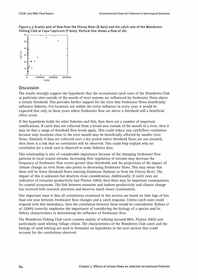
Cape Capricorn The scatter plot shows that years where annual Fitzroy River flow was greater than 1 GL were more closely related to catch rate than below this figure (Figure 5.3). Flow was more closely correlated with catch rate above 1 GL (r=0.91) than below (r=0.003).
Chapter 5. Effects of stream flows on selected recreational fisheries 83
CZCRC and FRDC Final Report Environmental Flows for Fisheries in Sub-tropical Estuaries
Figure 5.3 Scatter plot of flow from the Fitzroy River (X Axis) and the catch rate of the Wanderers Fishing Club at Cape Capricorn (Y Axis). Vertical line shows a flow of 1GL
Discussion The results strongly support the hypothesis that the recreational catch rates of the Wanderers Club at particular sites outside of the mouth of river systems are influenced by freshwater flows above a certain threshold. This provides further support for the view that freshwater flows beneficially influence fisheries. For locations not within the rivers influence in every year, it would be expected that only in those years where freshwater flow are above a threshold will a beneficial effect occur.
If this hypothesis holds for other fisheries and fish, then there are a number of important ramifications. If catch data are collected from a broad area outside of the mouth of a river, then it may be that a range of threshold flow levels apply. This could reduce any catch/flow correlation because only locations close to the river mouth may be beneficially affected by smaller river flows. Similarly if data are collected over a dry period where threshold flows are not attained, then there is a risk that no correlation will be observed. This could help explain why no correlation (or a weak one) is observed in some fisheries data.
This relationship is also of considerable importance because of the changing freshwater flow patterns in local coastal streams. Increasing flow regulation of streams may decrease the frequency of freshwater flow events greater than thresholds and the projections of the impact of climate change on river flows also points to decreasing freshwater flows. This may mean that there will be fewer threshold flows entering Gladstone Harbour or from the Fitzroy River. The impact of this is unknown but deserves close consideration. Additionally, if catch rates are indicative of estuarine productivity (see Platten 2005), then there may be important consequences for coastal ecosystems. The link between estuarine and inshore productivity and climate change has received little research attention and deserves much closer examination.
One important issue is that all correlations examined in this section are based on time lags of less than one year between freshwater flow changes and a catch response. Unless catch rates could respond with this immediacy, then the correlation between them would be coincidental. Robins et al. (2005) correctly emphasise the importance of considering the biology of a species and its fishery characteristics in determining the influence of freshwater flow.
The Wanderers Fishing Club catch consists mainly of whiting (around 80%, Platten 2005) and particularly sand whiting Sillago ciliata. The characteristics of the Wanderers Club catch and the biology of sand whiting are used to formulate an hypothesis in the next section that could account for the correlations observed.
Chapter 5. Effects of stream flows on selected recreational fisheries 84

CZCRC and FRDC Final Report Environmental Flows for Fisheries in Sub-tropical Estuaries
Hypothesis 3. Club catch rates respond relatively rapidly to threshold flows through changes in growth rate of whiting close to the minimum legal size Robins et al. (2005) review proposed mechanisms for freshwater flows influencing estuarine fishery production. These might be summarised as:
1) Changes in food availability related to nutrient enrichment associated with freshwater flows;
2) Changes in distribution related to translocation or alteration of habitat. This may cause fish to become more available to fisheries; and
3) Changes to population dynamics associated with factors such as growth, recruitment and survival.
They propose an integrated approach for examining the flow/catch relationship that involves both (i) an examination of the fishery characteristics, life history, and biology of the species to attempt to hypothesise how flow could influence these factors; and (ii) examination of catch and flow statistics for evidence to support this view.
In order to examine whether the catch rates of the Wanderers Fishing club could respond in the manner suggested from the correlations of catch and flow, it is thus necessary to briefly examine the characteristics of the clubs catch and the biology of the key species. The catch of the Wanderers Fishing Club is dominated by whiting, Sillago spp. (around 80% of the catch, Platten 2004, 2005). Observations of the catch from several outings suggest that all of the whiting caught were sand whiting (Sillago ciliata). Any rapid changes in catch rates are likely to be based around changes in the catch of this species.
Sand whiting feed on benthic macro-invertebrates (Burchmore et al. 1988). They grow relatively rapidly and may mature in their first year of life at around 24 cm in length (Burchmore et al. 1988). Sand whiting are most commonly found on sandy substrates or associated with seagrass (Burchmore et al. 1988). Currie and Small (2005) examined macro-benthos abundance (the principal food group used by sand whiting) at a number of sites in Port Curtis. This abundance is closely correlated (r=0.967) to the catch rates of the Wanderers Club (see Platten 2005 for a more detailed examination), suggesting that it is at least possible that changes in catch rate could be related to changes in food abundance.
Whiting are the most common species of fish taken by recreational fishers in Queensland (Higgs 1998). The catch of the species was regulated by a minimum size limit of 23 cm total length (TL) at the time of this study.
There is no information available that links sand whiting catch or biology to freshwater flows. However, examination of the three causal mechanisms suggests some possibilities. These are summarised as follows as a conceptual framework for further examination:
1) Changes in food availability: Increased nutrient input related to larger freshwater flows could provide the basis for improved primary production and ultimately increased food availability via the food chain. This could increase growth rates and or result in increased survival. This could increase the numbers of whiting available to the fishery;
2) Changes in movement patterns or habitat resulting from increased freshwater flow: Whiting could move away from locations of lower salinity or in response to other changes in habitat related to increased freshwater flow. This could result in more fish being available at the fishing locations (at least temporarily);
3) Changes to population dynamics associated with factors such as growth, recruitment and survival: Increased growth rate related to increased food availability linked to increases in nutrient, resulting in more fish reaching or surviving to legal size and hence becoming available to the fishery.
Chapter 5. Effects of stream flows on selected recreational fisheries 85

CZCRC and FRDC Final Report Environmental Flows for Fisheries in Sub-tropical Estuaries
The first and third causal mechanisms are obviously linked. They might be aggregated to a single causal mechanism suggesting increased nutrient supply could result in increased growth, survival and recruitment to the fishery. Thus, this causal mechanism requires a biological population dynamics response to freshwater flow inputs (positive growth and or survival). To test this hypothesis, information related to the age, growth and survival of sand whiting at the sites and the age structure of the catch would assist. Further information linking changes in food availability to catch rates and changes in the size structure of the catch related to freshwater flow would also assist. The second causal mechanism requires no positive growth or survival response. Increased catches should be based around increased abundance of individuals with similar size structures.
In order to examine possible causes for a catch rate/flow correlation, a limited analysis of the age structure of the catch was conducted.
Methods A random sample of 257 whiting frames was collected from the catch of Wanderers Fishing Club at Cape Capricorn. The length (cm, length to caudal fork (FL)) and sex of the fish were recorded and the otoliths removed from the heads. The otoliths were aged by the staff of the Department of Primary Industries and Fisheries at the Southern Fisheries Centre Deception Bay (see Chapter 6; Staunton-Smith et al. 2004).
Estimated age and measured length were compared and the catch curve of the percentage frequency of fish at age used to illustrate mortality. A model was constructed using least squares regression between log(e) transformed percentage frequency and age. From this, the residuals between the fitted and observed values were calculated and compared with freshwater flow data from the Fitzroy River for the back-calculated year of spawning i.e. year of sampling = predicted age (see Chapter 6; Staunton-Smith et al. 2004).
Results The relationship between estimated age and fish length is illustrated in Figure 5.5. This plot shows that 87% of sand whiting captured were between 210 and 250 mm FL. This is clustered around the legal minimum length of 230 mm total length (= approximately 210 mm FL). In fact, the largest size class of fish was between 210 and 220 mm FL (30.4% of fish) and 55.6% of fish were less than 230 mm FL (Figure 5.4). This indicates that the number of fish just over legal length particularly affects the catch rates.
Figure 5.4 Size distribution of sand whiting within the sample of fish from the catch of the Wanderers Fishing Club
Size composition of whiting catch
0
5
10
15
20
25
30
35
210-220 221-230 231-240 241-250 251-260 261-270 271-280 281-290 291-300
Size classes (mm FL)
% F
requ
ency
Chapter 5. Effects of stream flows on selected recreational fisheries 86
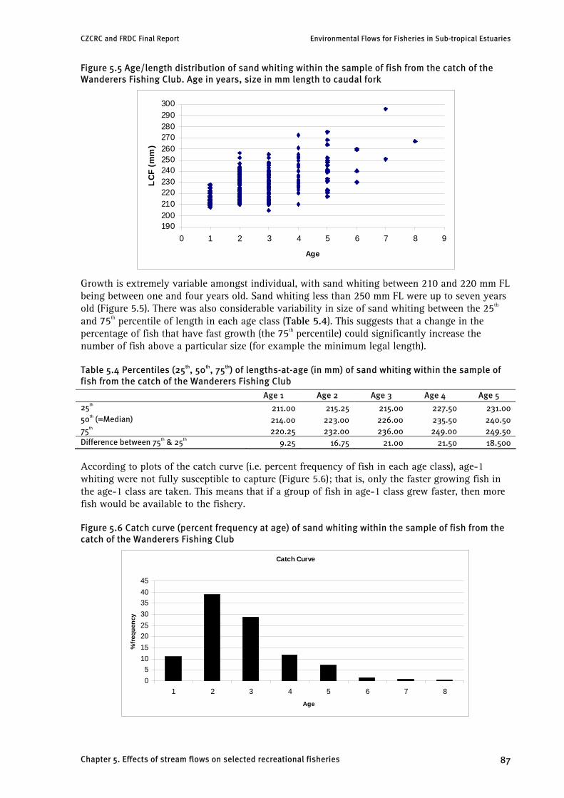
CZCRC and FRDC Final Report Environmental Flows for Fisheries in Sub-tropical Estuaries
Figure 5.5 Age/length distribution of sand whiting within the sample of fish from the catch of the Wanderers Fishing Club. Age in years, size in mm length to caudal fork
190 200 210 220 230 240 250 260 270 280 290 300
0 1 2 3 4 5 6 7 8 9
Age
LC
F (m
m)
Growth is extremely variable amongst individual, with sand whiting between 210 and 220 mm FL being between one and four years old. Sand whiting less than 250 mm FL were up to seven years old (Figure 5.5). There was also considerable variability in size of sand whiting between the 25th
and 75th percentile of length in each age class (Table 5.4). This suggests that a change in the percentage of fish that have fast growth (the 75th percentile) could significantly increase the number of fish above a particular size (for example the minimum legal length).
Table 5.4 Percentiles (25th, 50th, 75th) of lengths-at-age (in mm) of sand whiting within the sample of fish from the catch of the Wanderers Fishing Club
Age 1 Age 2 Age 3 Age 4 Age 5 25th
211.00 215.25 215.00 227.50 231.00 50th (=Median) 214.00 223.00 226.00 235.50 240.50 75th 220.25 232.00 236.00 249.00 249.50 Difference between 75th & 25th
9.25 16.75 21.00 21.50 18.500
According to plots of the catch curve (i.e. percent frequency of fish in each age class), age-1 whiting were not fully susceptible to capture (Figure 5.6); that is, only the faster growing fish in the age-1 class are taken. This means that if a group of fish in age-1 class grew faster, then more fish would be available to the fishery.
Figure 5.6 Catch curve (percent frequency at age) of sand whiting within the sample of fish from the catch of the Wanderers Fishing Club
Catch Curve
0 5
10 15 20 25 30 35 40 45
1 2 3 4 5 6 7 8 Age
%fr
eque
ncy
Chapter 5. Effects of stream flows on selected recreational fisheries 87
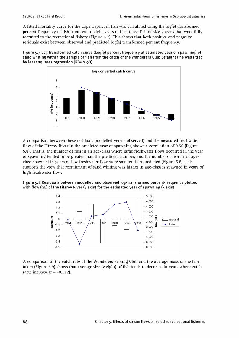
log converted catch curve
-2
-1
0
1
2
3
4
5
2001 2000 1999 1998 1997 1996 1995 1994
ln(%
freq
uenc
y)
CZCRC and FRDC Final Report Environmental Flows for Fisheries in Sub-tropical Estuaries
A fitted mortality curve for the Cape Capricorn fish was calculated using the log(e) transformed percent frequency of fish from two to eight years old i.e. those fish of size-classes that were fully recruited to the recreational fishery (Figure 5.7). This shows that both positive and negative residuals exist between observed and predicted log(e) transformed percent frequency.
Figure 5.7 Log transformed catch curve (Log(e) percent frequency at estimated year of spawning) of sand whiting within the sample of fish from the catch of the Wanderers Club Straight line was fitted by least squares regression (R2 = 0.98).
A comparison between these residuals (modelled versus observed) and the measured freshwater flow of the Fitzroy River in the predicted year of spawning shows a correlation of 0.56 (Figure 5.8). That is, the number of fish in an age-class where large freshwater flows occurred in the year of spawning tended to be greater than the predicted number, and the number of fish in an age-class spawned in years of low freshwater flow were smaller than predicted (Figure 5.8). This supports the view that recruitment of sand whiting was higher in age-classes spawned in years of high freshwater flow.
Figure 5.8 Residuals between modelled and observed log-transformed percent-frequency plotted with flow (GL) of the Fitzroy River (y axis) for the estimated year of spawning (x axis)
-0.5
-0.4
-0.3
-0.2
-0.1
0
0.1
0.2
0.3
0.4
1994 1995 1996 1997 1998 1999 2000
Res
idua
l
0.000
0.500
1.000
1.500
2.000
2.500
3.000
3.500
4.000
4.500
5.000
Flow
(GL)
residual Flow
A comparison of the catch rate of the Wanderers Fishing Club and the average mass of the fish taken (Figure 5.9) shows that average size (weight) of fish tends to decrease in years where catch rates increase (r = -0.512).
Chapter 5. Effects of stream flows on selected recreational fisheries 88
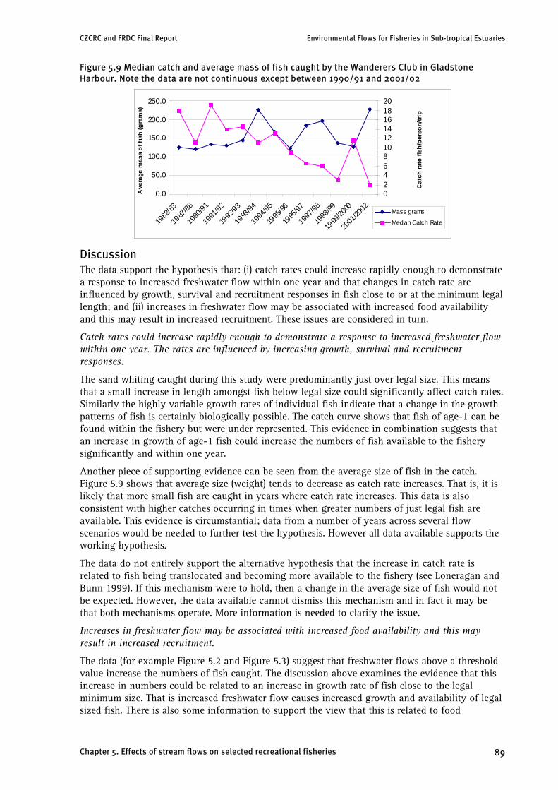
CZCRC and FRDC Final Report Environmental Flows for Fisheries in Sub-tropical Estuaries
Figure 5.9 Median catch and average mass of fish caught by the Wanderers Club in Gladstone Harbour. Note the data are not continuous except between 1990/91 and 2001/02
0. 0
50 .0
10 0 . 0
15 0 . 0
20 0 . 0
25 0 . 0
1982
/83
1987
/88
1990
/91
1991
/92
1992
/93
1993
/94
1994
/95
1995
/96
1996
/97
1997
/98
1998
/99
1999
/2000
2001
/2002
Ave
rage
mas
s of
fish
(gra
ms)
0 2 4 6 8 10 12 14 16 18 20
Cat
ch ra
te fi
sh/p
erso
n/tri
p
M a s s gr am s
M e di an C at c h R at e
Discussion The data support the hypothesis that: (i) catch rates could increase rapidly enough to demonstrate a response to increased freshwater flow within one year and that changes in catch rate are influenced by growth, survival and recruitment responses in fish close to or at the minimum legal length; and (ii) increases in freshwater flow may be associated with increased food availability and this may result in increased recruitment. These issues are considered in turn.
Catch rates could increase rapidly enough to demonstrate a response to increased freshwater flow within one year. The rates are influenced by increasing growth, survival and recruitment responses.
The sand whiting caught during this study were predominantly just over legal size. This means that a small increase in length amongst fish below legal size could significantly affect catch rates. Similarly the highly variable growth rates of individual fish indicate that a change in the growth patterns of fish is certainly biologically possible. The catch curve shows that fish of age-1 can be found within the fishery but were under represented. This evidence in combination suggests that an increase in growth of age-1 fish could increase the numbers of fish available to the fishery significantly and within one year.
Another piece of supporting evidence can be seen from the average size of fish in the catch. Figure 5.9 shows that average size (weight) tends to decrease as catch rate increases. That is, it is likely that more small fish are caught in years where catch rate increases. This data is also consistent with higher catches occurring in times when greater numbers of just legal fish are available. This evidence is circumstantial; data from a number of years across several flow scenarios would be needed to further test the hypothesis. However all data available supports the working hypothesis.
The data do not entirely support the alternative hypothesis that the increase in catch rate is related to fish being translocated and becoming more available to the fishery (see Loneragan and Bunn 1999). If this mechanism were to hold, then a change in the average size of fish would not be expected. However, the data available cannot dismiss this mechanism and in fact it may be that both mechanisms operate. More information is needed to clarify the issue.
Increases in freshwater flow may be associated with increased food availability and this may result in increased recruitment.
The data (for example Figure 5.2 and Figure 5.3) suggest that freshwater flows above a threshold value increase the numbers of fish caught. The discussion above examines the evidence that this increase in numbers could be related to an increase in growth rate of fish close to the legal minimum size. That is increased freshwater flow causes increased growth and availability of legal sized fish. There is also some information to support the view that this is related to food
Chapter 5. Effects of stream flows on selected recreational fisheries 89

CZCRC and FRDC Final Report Environmental Flows for Fisheries in Sub-tropical Estuaries
availability. Sand whiting are largely second order consumers (Burchmore et al. 1988) feeding on benthic macro-invertebrates. Currie and Small (2005) and Platten (2005) demonstrate that the abundance of macro-benthos is closely related to catch rates in Gladstone Harbour. It is possible that the response in catch rates is reflecting changes in food availability. Currie and Small (2005) propose that changes in nutrient supply are associated with changes in macro-benthos abundance. Thus, it is likely that increased nutrient supply associated with freshwater flows could also positively influence both macro-benthos abundance and recreational fishing club catch rates and requires further research.
Discussion To establish a link between freshwater flow and the catch of whiting is important because whiting are the most frequently captured recreational fishing species in Queensland, Australia (Higgs 1998; Henry and Lyle 2003). In addition, the findings of this chapter add to the knowledge relating to the influence of freshwater flow on fisheries in several ways.
There is strong evidence that freshwater flows positively influence the line fishing catch of whiting in both Gladstone Harbour and at Cape Capricorn. Demonstrating the relationship between whiting catches and freshwater flow adds another species at another trophic level to the body of evidence that demonstrates the positive influence of freshwater flows on fisheries.
The findings are also the first to demonstrate that at a particular site, a freshwater flow threshold may be required before a defined flow/catch correlation exists. This evidence is important because it offers one explanation as to why a clear flow/catch relationship may not be obvious. For example, Gartside et al. (1999) found no correlation between recreational catch rates and river floods, but their data was from a broad area and only an overall correlation between flood volumes and catches was sought i.e. no analysis using a technique likely to demonstrate threshold effects was conducted. It is suggested that an analysis across a broad range of flow regimes over a long time frame is necessary to clearly establish any freshwater flow/catch relationship. An approach that seeks possible threshold freshwater flow values is also warranted. Similarly, the location of fishing appears to influence any freshwater flow/catch correlation. It seems likely that data from a closely defined fishing location will provide the best opportunity to establish a definite correlation.
The chapter also points to another likely causal mechanism to explain why catch rates could be influenced by freshwater flow. Unlike several other fisheries, the response to freshwater flow seems relatively immediate. That is, the strongest correlation exists with freshwater flow of the same year. This does not mean there is no lagged effect, but that the lag period is less than one year. This fits with the biology of the species (i.e. sand whiting) and the characteristics of the recreational club fishery. Catch rates are particularly influenced by the numbers of fish just over legal minimum size. This combined with the variability in growth rates provides a likely explanation for why the catch rate could respond in the way observed. There is strong evidence to suggest that the catch response is related to increased recruitment of whiting related to more fish just above legal minimum size becoming available. There is also evidence to suggest that this may be related to food availability and associated changes in growth rate. The view proposed by Robins et al. (2005) that it is important to examine the biology of fish species and fishery characteristics to gain an understanding as to why a correlation exists is supported.
The information examined supports the view that the freshwater flow/catch relationship for sand whiting is influenced by the number of fish caught, rather than an increase in the size of fish. This aspect is not always obvious from commercial catch data where catch records are based on the weight of landed product rather than the numbers of fish. It is possible that a positive influence of freshwater flow on the numbers of fish caught may be masked within records that only record landed weights since catch weight may not increase (or even decrease) in response to more small fish being captured. This could be a further factor masking a freshwater flow/catch
Chapter 5. Effects of stream flows on selected recreational fisheries 90

CZCRC and FRDC Final Report Environmental Flows for Fisheries in Sub-tropical Estuaries
correlation. It is suggested that wherever possible both landed weight and the numbers of fish caught should be analysed.
The implications of the freshwater flow/catch correlation may extend well beyond a positive influence on catch rates. The close relationship between macro-benthos abundance and catch rates suggests that catch trends could be indicative of broader ecological productivity changes (see Platten 2004, 2005). Whiting are likely to be integral to a range of trophic inter-relationships. If this is so, then freshwater flows may influence the productivity of most of the estuarine ecosystem. This is of particular significance given both the predicted changes in rainfall patterns related to climate change and the increasing regulation of streams. This aspect is deserving of much greater research effort.
Chapter 5. Effects of stream flows on selected recreational fisheries 91