Cyclone Warning Division India Meteorological Department ... · Arabian Sea during 28 October-04...

0

GOVERNMENT OF INDIA MINISTRY OF EARTH SCIENCES

EARTH SYSTEM SCIENCE ORGANISATION INDIA METEOROLOGICAL DEPARTMENT

Extremely Severe Cyclonic Storm, CHAPALA over the Arabian Sea (28 October - 4 November, 2015): A Report

Insat-3D Satellite imagery of 1500 UTC of 1 November 2015

Cyclone Warning Division

India Meteorological Department

New Delhi

December 2015

1

Extremely Severe Cyclonic Storm (ESCS) Chapala

over the Arabian Sea

(28 October - 04 November 2015)

1. Introduction

An Extremely Severe Cyclonic Storm (ESCS) 'Chapala' formed from a low pressure area over southeast Arabian Sea (AS) which concentrated into a depression in the morning of 28th October. It moved north-northwestwards and intensified into a deep depression in the same evening. It further intensified into a cyclonic storm in the early hours of 29th over eastcentral Arabian Sea. It then moved west-northwestwards, further intensified into a severe cyclonic storm in the evening and a very severe cyclonic storm in the midnight of 29th and into an extremely severe cyclonic storm in the morning of 30 th. It then moved mainly westwards, maintained its intensity till 1st November and then started weakening gradually. Moving west-northwestwards, it crossed Yemen coast to the southwest of Riyan (14.1/48.65) during 0100-0200 UTC of 3rd November as very severe cyclonic storm. It further westwards and weakened into a severe cyclonic storm in the morning , into a cyclonic storm by noon and into deep depression around midnight of 3rd November. it then weakened into a depression in the early morning of 4th and lay as well marked low pressure area over Yemen at 0300 UTC of 4th November. The salient features of this cyclone are as follows.

ESCS Chapala is the first severe cyclone to cross Yemen coast after the severe

cyclonic storm of May 1960.

The ESCS Chapala had a life period of 7 days , which is above normal (average life

period of VSCS/ESCS is 6 days in NIO and 4.7 days in Post monsoon season for

VSCS/ESCS)

It had the maximum intensity of 115 kts (215 kmph) and crossed Yemen coast with a

speed of 65 knots (120 kmph).

The system had the longest track length after VSCS Phet in 2010. It travelled a distance

of about 2248 km during its life period.

The Accumulated Cyclone Energy (ACE) was about 18.29 X 104 knot2 (the mean for the

period (1990-2013) in the post monsoon season over Arabian Sea is 0.8 X 104 knot2),

which is same as VSCS, Phet over Arabian Sea in 2010.

The Power Dissipation Index was 17.92 X 106 knot3 which is also same as that of VSCS

Phet in 2010 (the mean for the period (1990-2013) in the post monsoon season is 0.4 X

106 knot3.

The system rapidly intensified from 29th morning to 30th afternoon, when the speed

increased from 35 kts at 0000 UTC of 29th Oct to 90 kts at 0900 UTC of 30th Oct.

Though the system moved over to colder Gulf of Aden, experienced dry air intrusion

and interacted with the land surface, it did not weaken rapidly due to low vertical wind

shear around the centre and in the forward sector of the system.

There was large divergence and hence higher than normal errors in NWP models for

prediction of its track and intensity especially, the landfall over Yemen.

RSMC New Delhi predicted genesis on 25th October, 3 days in advance and its

intensification to ESCS one day in advance on 29th October 2015. The forecast of

2

landfall over Yemen and adjoining Oman coast was issued on the day of genesis i.e.,

28th Oct., 6 days advance and landfall over Yemen was issued on 31 Oct. with a lead

period of 5 days. Every 3 hourly Tropical Cyclone Advisory were issued to

WMO/ESCAP panel countries including Oman and Yemen & Somalia.

Brief life history, characteristic features and associated weather along with

performance of numerical weather prediction models and operational forecast of IMD

are presented and discussed in following sections.

2. Monitoring of ESCS, Chapala

The ESCS Chapala was monitored & predicted continuously since its inception

by the India Meteorological Department (IMD). The forecast of its genesis (formation of

Depression) on 28th October, its track, intensity, point & time of landfall was well

predicted by IMD. The system was monitored mainly by observations from satellite

throughout its life period. Various national and international NWP models and

dynamical-statistical models including IMD and National Centre for Medium Range

Weather Forecasting (NCMRWF) global and meso-scale models, dynamical statistical

models for genesis and intensity were utilized to predict the genesis, track and intensity

of the storm. Tropical Cyclone Module, the digitized forecasting system of IMD was

utilized for analysis and comparison of various models guidance, decision making

process and warning product generation.

3. Brief life history

3.1. Genesis

During the onset phase of northeast monsoon, a trough of low with embedded

upper air cyclonic circulation in lower levels lay over southeast Bay of Bengal on 25th

Oct. Under its influence, a low pressure area formed over southeast and adjoining

southwest and eastcentral Arabian Sea at 0300 UTC of 26th Nov. with associated

cyclonic circulation extending upto mid-tropospheric levels. It became well marked over

the same region at 0300 UTC of 27th morning. It concentrated into a depression over

southeast and adjoining southwest and central Arabian Sea at 0300 UTC of 28th

October near Lat. 11.5°N and Long. 65.0°E.

The winds were stronger in northern sector (25-30 knots) under the influence of

northeast monsoon current and were about 15-20 knots in other sectors as seen from

multi-satellite surface winds. The Sea Surface Temperature (SST) was about 30°C

around the region of depression. The vertical wind shear was moderate (10-20 knots)

around the system centre and was low (5-10 knots) to the west-northwest of the system

centre. The low level relative vorticity was about 100 x 10-5 second-1 and low level

convergence was 5-10 x 10-5 second-1. The upper level divergence was 30 x 10-5

second-1. The ocean thermal energy was about 60-80kJ/cm2. MJO lay in phase 2 (west

equatorial region) with amplitude greater than 2.

3.2. Track and intensification

Best track parameters of ESCS, Chapala over AS (28th Oct.-4nd Nov., 2015) are

given in Table 1. The observed track of the system is also shown in Fig. 1.

3

Fig. 1 Observed track of ESCS Chapala during 28th Oct. to 04th Nov 2015.

The environmental features and large scale features as mentioned in the

previous section continuously favoured the intensification of the system during 28th -30

Oct. The system rapidly intensified from 29th to 30th, when the speed increased from

35 kts at 0000 UTC of 29th Oct to 90 kts at 0900 UTC of 30th Oct. There was land

interaction and impact of dry air intrusion from northwest from 01 Nov. onwards.

However, the impact of dry air intrusion from northwest and land interaction was slow

because of low vertical wind shear to the west and west-southwest of the system as can

be seen in Fig. 2 and hence the system could maintain its intensity of ESCS from 0000

UTC of 30th Oct. to 0900 UTC of 2 Nov. The Total Precipitable Water (TPW) imageries

during 28 Oct. to 04 Nov. is shown in Fig. 4 which clearly exemplifies the low impact of

dry air intrusion into the wall cloud region. From 0300 UTC of 2nd Nov. The system

started interacting with land surface and also the convection in the wall cloud region

showed signs of disorganisation indicating the weakening trend of the system. It

crossed Yemen coast to the southwest of Riyan (14.1/48.65) during 0100-0200

UTC of 3rd November as Very Severe Cyclonic Storm (VSCS). It then weakened

rapidly into SCS at 0300 UTC, into a CS at 0600 UTC and into a Deep Depression (DD)

at 1800 UTC on the same day due to land interaction. It further weakened into a

Depression at 0000 UTC and into a well marked low pressure area at 0300 UTC of 4 th

November 2015 over Yemen.

4

The system initially moved north-northwestwards in association with the anti-cyclonic

circulation lying to the northeast of the system centre. It then came under the influence

of another anti-cyclonic circulation to its northwest on 29th which increased westward

component in the movement of the system. The system lay in the south eastern

periphery of this anticyclone. Thus the system moved nearly westwards to west-

southwestward upto 0300 UTC of 2 Nov. It then lay to the southwest of the anticyclone

and the ridge (Lat. 16°N) at 200 hPa and thus moved west-northwestwards towards

Yemen coast. It moved normally with a speed of 13 kmph initially, its speed gradually

picked up and became about 20 kmph on the day before landfall. The direction and

translational speed of movement of the system is illustrated in Fig. 3.

Fig. 2. Wind shear and wind speed in the middle and deep layer around the

system during 28th Oct. to 05th Nov 2015.

Fig. 3. Translational speed and direction of ESCS Chapala during 28th Oct. to 04th

Nov 2015.

5

Fig.4 TPW imageries of ESCS Chapala during 28th Oct. to 04th Nov 2015.

28 Oct. 1933 UTC 29 Oct. 0445 UTC

29 Oct. 1637 UTC 30 Oct. 0423 UTC

31 Oct. 0132 UTC 31 Oct. 2254 UTC

6

Fig. 4 contd. TPW imageries of ESCS Chapala during 28th Oct. to 04th Nov 2015.

01 Nov. 0733 UTC 01 Nov. 1655 UTC

02 Nov. 0145 UTC 02 Nov. 1052 UTC

03 Nov. 0443 UTC

04 Nov. 0151 UTC

7

Table 1: Best track positions and other parameters of ESCS CHAPALA over the Arabian Sea during 28 October-04 November, 2015

Date Time (UTC)

Centre lat.° N/

long. ° E

C.I. NO.

Estimated Central

Pressure (hPa)

Estimated Maximum Sustained Surface

Wind (kt)

Estimated Pressure

drop at the Centre (hPa)

Grade

28-10-2015

0300 11.5/65.0 1.5 1005 25 3 D

0600 11.8/64.9 2.0 1004 25 4 D

1200 12.5/64.7 2.0 1001 30 5 DD

1800 13.0/64.7 2.0 1001 30 5 DD

29-10-2015

0000 13.7/64.3 2.5 999 35 7 CS

0300 13.8/64.2 2.5 997 40 9 CS

0600 13.9/63.8 3.0 996 45 10 CS

0900 14.0/63.5 3.0 994 50 12 SCS

1200 14.1/63.3 3.5 990 55 16 SCS

1500 14.3/62.8 3.5 988 60 18 SCS

1800 14.3/62.5 4.0 984 65 22 VSCS

2100 14.3/62.3 4.5 976 75 30 VSCS

30-10-2015

0000 14.3/61.8 5.0 966 90 40 ESCS

0300 14.3/61.5 5.5 954 105 52 ESCS

0600 14.3/61.1 5.5 948 110 58 ESCS

30-10-2015

0900 14.2/60.8 6.0 940 115 66 ESCS

1200 14.1/60.6 6.0 940 115 66 ESCS

1500 14.0/60.4 6.0 940 115 66 ESCS

1800 13.9/60.2 6.0 940 115 66 ESCS

2100 13.9/59.9 6.0 942 115 64 ESCS

31-10-2015

0000 13.9/59.6 5.5 944 110 62 ESCS

0300 13.8/59.2 5.5 946 110 60 ESCS

0600 13.8/58.7 5.5 950 105 56 ESCS

0900 13.8/58.3 5.5 950 105 56 ESCS

1200 13.8/57.9 5.5 950 105 56 ESCS

1500 13.8/57.5 5.5 950 105 56 ESCS

1800 13.8/57.2 5.5 950 105 56 ESCS

2100 13.7/56.8 5.5 950 105 56 ESCS

01-11-2015

0000 13.7/56.4 5.5 950 105 56 ESCS

0300 13.6/56.1 5.5 952 105 54 ESCS

0600 13.6/55.6 5.5 954 100 52 ESCS

0900 13.6/55.1 5.5 956 100 50 ESCS

1200 13.6/54.6 5.5 956 100 50 ESCS

1500 13.6/54.2 5.5 956 100 50 ESCS

1800 13.4/53.7 5.5 956 100 50 ESCS

2100 13.3/53.1 5.5 956 100 50 ESCS

8

02-11-2015

0000 13.2/52.5 5.5 958 100 48 ESCS

0300 13.2/52.2 5.0 960 95 46 ESCS

0600 13.3/51.6 5.0 964 90 42 ESCS

0900 13.3/51.0 5.0 966 90 40 ESCS

1200 13.4/50.5 4.5 968 85 38 VSCS

1500 13.5/50.0 4.5 970 85 36 VSCS

1800 13.7/49.6 4.5 974 80 32 VSCS

2100 13.8/49.3 4.0 978 75 28 VSCS

3-11-2015

0000 14.0/48.8 4.0 984 65 22 VSCS

Crossed Yemen coast to the southwest of Riyan (14.1/48.65) during 0100-0200 UTC.

0300 14.2/48.4 - 990 55 16 SCS

0600 14.2/47.8 - 996 45 10 CS

0900 14.2/47.6 - 998 40 8 CS

1200 14.2/47.3 - 998 40 8 CS

1500 14.2/47.1 - 998 40 8 CS

1800 14.3/47.0 - 1001 30 5 DD

04-11-2015

0000 14.8/46.5 - 1003 25 3 D

0300 Well marked low pressure area over Yemen.

3.3. Maximum Sustained Surface Wind speed and estimated central pressure:

The lowest estimated central pressure has been 940 hPa. The estimated

maximum sustained surface winds (MSW) was 115 knots during 0900 - 2100 UTC of

30th Oct. However, at the time of landfall, the ECP was 984 hPa and MSW was 65

knots (very severe cyclonic storm) due to weakening of the system over Gulf of Aden.

Fig. 5 Estimated Central Pressure (ECP) and estimated maximum sustained

surface wind speed during 28th Oct./0300 UTC to 04th Nov/0000 UTC.

9

It can be seen from Fig.5 that there was rapid intensification from 29/0000 UTC to

30/0900 UTC.

4. Climatological aspects

Climatologically, the severe cyclonic storms crossing Yemen coasts are very rare.

Prior to Chapala, only one SCS in May 1960 crossed Yemen coast during the 1891-

2014). The track of the SCS is shown in Fig.6.

Fig. 6 Tracks of Severe cyclonic storm over Arabian Sea during the period 1891-

2014 that crossed Yemen coast.

5. Features observed through satellite

(a) INSAT 3D and Kalpana imageries:

Half hourly Kalpana-1 and INSAT-3D imageries were utilised for monitoring of

ESCS, Chapala. Satellite imageries of international geostationary satellites Meteosat-7

and MTSAT and microwave & high resolution images of polar orbiting satellites DMSP,

NOAA series, TRMM, Metops were also considered. Typical satellite INSAT-3D

imageries (IR, visible, IRBD and enhanced colour imageries) of ESCS Chapala

representing the life cycle of the cyclone are shown in Fig. 7-10.

As per the satellite imageries, on 26th October, broken low and medium clouds

with embedded intense to very intense convection lay over south Arabian Sea between

equator to latitude 10.0°N and longitude 61.0°E to 74.0°E in association with the low

pressure area over the area.

10

On 27th/0300, vortex was observed over south Arabian Sea centered within half a

degree of latitude 8.5˚N and longitude 66.0˚E with intensity T1.0 and poorly defined

centre. Associated broken low and medium clouds with embedded moderate to intense

convection lay over the area between latitude 6.0˚N to 14.5˚N and longitude 60.0˚E to

72.0˚E. The lowest cloud top temperature (CTT) associated with the vortex was -70°C.

On 28th/0300 UTC, intensity of the system was T1.5 with convective clouds showing

shear pattern and increase in organisation. On 28th/1200 UTC, the intensity of the

system became T2.0 with increased convection and organisation into curved band

pattern during the past 12 hours.

On 29th, the intensity of the system increased rapidly by three T numbers in 24

hrs. At 29/0000 UTC, the intensity of the system was T.2.5. At 29/0300 UTC, it became

T3.0, at 1200 UTC,T3.5 and at 1800 UTC of the same day, it was T4.0 and eye started

appearing. On 30th/0000 UTC, intensity further increased to T5.5 with convective cloud

showing eye pattern with well-defined eye of diameter about 15 km in both visible and

IR imageries. By 0900 UTC of 30th, intensity further increased to T6.0 with well-defined

eye of diameter about 15 km. At 2100 UTC of the same day, the eye pattern became

ragged. By 31st/0000 UTC, intensity became T5.5 / CI 6.0 and the eye was ragged. At

0600 UTC of the same day, intensity became T5.0 / CI 6.0. However, ragged eye was

observed in both visible and IR imageries. Minimum wall cloud temperature was -80°C.

By 0900 of the same day, weakening trend was observed in the associated convection.

At 1200 UTC of 31st, eye was defined in visible and IR imageries. At 1800 UTC of the

same day, minimum wall cloud temperature was -77°C. There was a good poleward

outflow from 0000 UTC of 29th Oct. which changed to radial outflow from 0000 UTC of

31st Oct. The poleward outflow again was seen from 1200 UTC of 01st Nov. to 0000

UTC of 2nd Nov.

On 01st November/0300 UTC, ragged eye re-appeared and the minimum wall

cloud temperature was -90°C. At 0300 UTC of the same day, intensity slightly

decreased to T5.5/ CI 5.5 and convection showed ragged eye pattern. On 2nd/0000

UTC, the eye diameter increased to about 45 km. At 0300 UTC of the same day,

intensity decreased to T5.0/ CI 5.5 and convection in the wall cloud region started

showing disorganisation. At 1200 UTC of the same day, intensity further decreased to

T4.5/ CI 5.5. However, well defined ragged eye was observed in both visible and IR

imageries. At 2100 UTC, the intensity further decreased to T4.0 / CI 4.5 and on

03rd/0000 UTC, convection was sheared to the northwest due to increase in vertical

wind shear and further disorganisation continued till day of landfall.

11

Fig. 7(a-g): INSAT 3D IR Imageries during 28 Oct.-4 Nov. 2015 based on 0600 UTC.

(a) 28 Oct. / 0600 UTC (b) 29 Oct. / 0600 UTC

(c) 30 Oct. / 0600 UTC (d) 31 Oct. / 0600 UTC

(e) 1 Nov. / 0600 UTC (f) 2 Nov. / 0600 UTC

(g) 3 Nov. / 0600 UTC

12

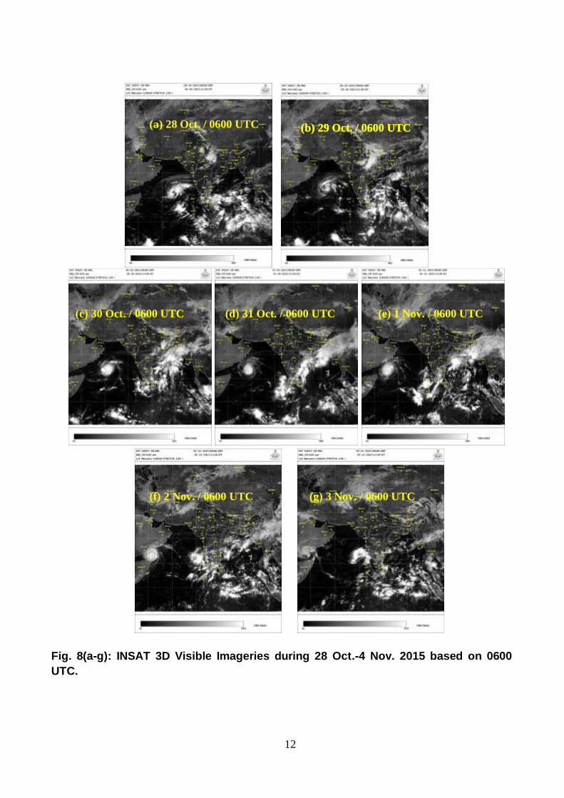
Fig. 8(a-g): INSAT 3D Visible Imageries during 28 Oct.-4 Nov. 2015 based on 0600

UTC.

(a) 28 Oct. / 0600 UTC (b) 29 Oct. / 0600 UTC (b) 29 Oct. / 0600 UTC

(c) 30 Oct. / 0600 UTC (d) 31 Oct. / 0600 UTC (e) 1 Nov. / 0600 UTC

(f) 2 Nov. / 0600 UTC (g) 3 Nov. / 0600 UTC

13

Fig. 9(a-e): INSAT 3D Imageries during 28 Oct. - 4 Nov. 2015 based on 0600 UTC.

(a) 28 Oct. / 0600 UTC (b) 29 Oct. / 0600 UTC (c) 30 Oct. / 0600 UTC

(d) 31 Oct./ 0600 UTC (e) 01 Nov / 0600 UTC

(f) 02 Nov. / 0600 UTC (g) 03 Nov. / 0600 UTC

14

Fig. 10(a-g): INSAT 3D enhanced imageries during 28 Oct. - 4 Nov. 2015 based on

0600 UTC.

(d) 31 Oct. / 0600 UTC (e) 01 Nov. / 0600 UTC

(f) 02 Nov. / 0600 UTC (g) 03 Nov. / 0600 UTC

(c) 30 Oct. / 0600 UTC (a) 28 Oct. / 0600 UTC (b) 29 Oct. / 0600 UTC

15

(f) SSMIS-31/0032 UTC

(a) SSMIS-28/0242 UTC

(c) SSMIS-29/1446 UTC (b) AMSR2-28/2126 UTC

(d) SSMIS-30/0322 UTC

(e) AMSR2-30/0900

UTC

(j) SSMIS-01/1115 UTC

(g) SSMIS-31/1453 UTC (h) SSMIS-01/0019 UTC (i) SSMIS-01/0330 UTC

(k) SSMIS-01/1550 UTC (l) SSMIS-02/1059 UTC

(m) SSMIS-02/2334 UTC Fig.11(a-m). Evolution of TC Chapala during 28 Oct - 03 Nov 2015 based on microwave imageries (SSMIS / AMSR2).

16

(b) Microwave features and eye characteristics Fig.11(a-m) presents the SSMIS / AMSR2 microwave imageries depicting the

organisation of convective clouds associated with the system. As seen, on 28 th October,

convective clouds organised from shear pattern to curved band pattern (a&b: 28/0242 &

28/2126). On 29th, curved banding improved considerably and eye feature started

appearing (c: 29/1446 UTC). Subsequently, as the system intensified, the eye feature

became very well-defined and eye wall completely covered the eye (d: 30/0322 UTC).

However, by 30/0900 UTC, the eye wall started opening (e), the eye became more and

more exposed and an outer eye wall started forming on 31st (f: 31/0032 UTC).

Thereafter, on 31/1453 UTC, the outer eye wall is observed to have shifted inwards

towards the partially dissolved inner eye wall (g). On 1st November, by 01/0019 UTC,

the inner eye wall has disappeared and the outer eye wall surrounds the eye (h).

Associated with this eye wall replacement cycle, there has been a temporary weakening

of the system on 30th. With the formation and strengthening of the secondary eye wall

(i: 01/0330 UTC), the intensity of the system increased further on 31st October and 01st

November (j:01/1115 UTC). On 01/1530 UTC, the outer eye wall completely surrounds

the eye and the system attained its mature stage (k). The eye diameter during this stage

was about 37 km. Subsequently, by 02/0300 UTC, the intensity of the system started

decreasing and at 02/1059 UTC, most of the wall cloud portion had dissolved and a

partial eye wall with an exposed eye is seen (l). As the system approached close to the

coast, further disorganisation occurred due to land interaction (m: 02/2334 UTC).

6. Surface wind structure

Fig. 12: Radius 34 knot (R34), radius of 50 knot (R50) & radius of 64 knot (R64), estimated maximum sustained surface winds (Vmax in knots) and Radius of Maximum winds (Rmax in nautical mile) based on multi-satellite surface wind (http://rammb.cira.colostate.edu/)

17

The surface wind structure during the life period of ESCS, Chapala based on multi-

satellite surface wind developed by CIRA, USA is shown in Fig. 12. It can be seen that

the radius of 34 kt (outer core size) winds was higher in northeast (NE) sector. It was

maximum of about 120 nm during its mature stage. Also in the radius of 50 kt/64 kt

(inner core size), the winds were higher in the northeastern sector as compared to the

other sector. Further it can be seen that the size of the outer core gradually increased

till 0600 UTC of 30th Oct., then it slightly decreased upto 1800 UTC of 30 Oct. followed

by a sharp increase upto 0000 UTC of 1st Nov. The size then almost remained same

upto 0000 UTC of 2nd Nov. and then gradually decreased. The change in the inner core

(R50) was similar to that of R34 and the temporal variation in R64 was less. Similarly

the Radius of Maximum Winds (RMW) did not show significant variation throughout the

TC stage and it varied from 15-20 nm.

7. Dynamical features

The genesis of the system took place on 28th under favourable environmental

conditions of high SST (around 30°C), low to moderate wind shear (10-20 knots),

conducive MJO conditions (phase 2 and amplitude greater than 1).

The system was initially located along the southwestern periphery of an

anticyclone to the northeast which steered the system northward / north-northwestward

on 28th. Subsequently, from 29th onwards, the system was steered by another anti-

cyclone located to the northwest of its centre. On 29th October, the system was located

along the southeastern periphery of the western anti-cyclone which steered the system

westward to west-southwestward and subsequently, during 30th October to 01st

November also the system was tracking west to west-southwestward under its

influence. On 2nd, the system centre was located along the southwestern periphery of

this anti-cyclone and was steered west-northwestward to northwestward on 2nd and 3rd

November.

During the period 28th October to 01 November, outflow above the system

centre strengthened significantly. On 29th, the poleward outflow increased and

subsequently, during 30th October to 01st November, the outflow from the system

centre was enhanced radially in all directions due to significant favourable interaction

with upper tropospheric trough and divergence associated with sub tropical westerly jet

located to the northeast of the system centre and the system continued to intensify

despite intrusion of cold air from the northwest. The system underwent rapid

intensification during 29/0000-30/00000 UTC in association with lowering of vertical

wind shear to about 5-10 knots near the system centre, enhanced poleward outflow

associated with an upper air westerly trough located to the northeast of the system

centre and continued prevalence of favourable MJO conditions. However, as the

system tracked more and more westwards towards Yemen coast on 2nd November, it

started weakening due to intrusion of cold and dry air and interaction with land.

Dynamical features observed in the IMD-GFS analysis of MSLP, 10m, 850 hPa,

500 hPa and 200 hPa winds based on 0000 UTC of 28-October to 03 November 2015

(Fig. 13 (i) to (vii)) are discussed herewith.

18

Fig 13 (i) : IMD-GFS analyses of (a) MSLP and winds at (b) 10 m (c) 850 hPa ,(d)

500 hPa & (e) 200 hPa levels based on 0000 UTC of 28th October, 2015

As seen, cyclogenesis of the system and its subsequent intensification is indicated by

the model. On 28th and 29th, surface winds of about 30-35 kts are predicted and winds

19

are stronger over the northeastern sector. The extent of subsequent intensification is

not indicated clearly by the model. However, major synoptic features associated with

movement and intensification of the system are predicted well. A deep amplitude

westerly trough at 500 hPa level is located north-northeast / northeast of the system

centre on 28th and 29th. At 200 hPa level, northeast-southwest oriented westerly trough

is located to the northeast of the system centre on 28th and 29th and poleward outflow

from the system merges with the sub-tropical westerly jet located to the northeast of the

system centre during 28th-31st. These features contributed significantly to enhanced

deepening of the central pressure and hence intensification of the system. On 31st,

associated with rapid intensification of the system, surface winds are symmetric about

the centre.

Fig 13(ii) : IMD-GFS analyses of (a)

MSLP and winds at (b) 10 m (c)

850 hPa ,(d) 500 hPa & (e) 200

hPa levels based on 0000 UTC of

29th October, 2015

20

Fig 13(iii) : IMD-GFS analyses of (a) MSLP and winds at (b) 10 m (c) 850 hPa ,(d)

500 hPa & (e) 200 hPa levels based on 0000 UTC of 30th October, 2015

21

Fig 13 (iv) : IMD-GFS analyses of (a) MSLP and winds at (b) 10 m (c) 850 hPa ,(d)

500 hPa & (e) 200 hPa levels based on 0000 UTC of 31st October, 2015

22

Fig 13 (v) : IMD-GFS analyses of (a) MSLP and winds at (b) 10 m (c) 850 hPa ,(d)

500 hPa & (e) 200 hPa levels based on 0000 UTC of 1st November, 2015

23

Fig 13 (vi) : IMD-GFS analyses of (a) MSLP and winds at (b) 10 m (c) 850 hPa ,(d)

500 hPa & (e) 200 hPa levels based on 0000 UTC of 2nd November, 2015

24

Fig 13 (vii) : IMD-GFS analyses of (a) MSLP and winds at (b) 10 m (c) 850 hPa ,(d)

500 hPa & (e) 200 hPa levels based on 0000 UTC of 3rd November, 2015

25

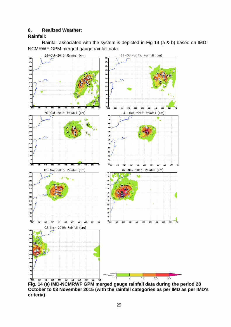
8. Realized Weather:

Rainfall:

Rainfall associated with the system is depicted in Fig 14 (a & b) based on IMD-

NCMRWF GPM merged gauge rainfall data.

Fig. 14 (a) IMD-NCMRWF GPM merged gauge rainfall data during the period 28 October to 03 November 2015 (with the rainfall categories as per IMD as per IMD's criteria)

26

During the initial stage of formation of the system, on 28th, rainfall belt was oriented along NE-SW and the rainfall maximum was observed to the northeast of the system centre. Subsequently, with the organisation of the system, convection became more and more organised and rainfall was symmetric about the centre on 31st. Rainfall of the order of 25-30 cm was realised near the core of the system on 28th and about 30-45 cm was realised in the wall cloud region during 29th October to 03rd November.

Fig. 14 (b) IMD-NCMRWF GPM merged gauge rainfall data during the period 28 October to 03 November 2015 9. Damage due to ESCS Chapala

As per media and press report, ESCS Chapala killed at least five people and

caused widespread damage as it brushed past Socotra Island of Yemen. More than

50,000 people in Yemen, including about 18,000 on Socotra, were displaced because of

Cyclone Chapala. Some photographs of damages caused by ECSC Chapala in Yemen are given in

Fig. 15.

Shore of Hadramout, damaged vehicles

due to heavy rains and winds Vehicles swept away by water in Socotra

27

Fig. 15: Damages caused due to ESCS Chapala over Yemen

10. NWP model forecast performance

IMD operationally runs a regional models, WRF for short-range prediction and

one Global model T574L64 for medium range prediction (7 days). The WRF-Var model

is run at the horizontal resolution of 27 km, 9 km and 3 km with 38 Eta levels in the

vertical and the integration is carried up to 72 hours over three domains covering the

area between lat. 25o S to 45o N long 40o E to 120o E. Initial and boundary conditions

are obtained from the IMD Global Forecast System (IMD-GFS) at the resolution of 23

km. The boundary conditions are updated at every six hours interval. The QLM model

(resolution 40 km) is used for cyclone track prediction in case of cyclone situation in the

north Indian Ocean. IMD also makes use of NWP products prepared by some other

operational NWP Centres like, ECMWF (European Centre for Medium Range Weather

Forecasting), GFS (NCEP), JMA (Japan Meteorological Agency). Hurricane WRF

(HWRF) model and Ensemble prediction system (EPS) has been implemented at the

NWP Division of the IMD HQ for operational forecasting of cyclones.

In addition to the above NWP models, IMD also run operationally dynamical

statistical models. The dynamical statistical models have been developed for (a)

Cyclone Genesis Potential Parameter (GPP), (b) Multi-Model Ensemble (MME)

technique for cyclone track prediction, (c) Cyclone intensity prediction, (d) Rapid

intensification and I Predicting decaying intensity after the landfall. Genesis potential

parameter (GPP) is used for predicting potential of cyclogenesis and forecast for

potential cyclogenesis zone. The multi-model ensemble (MME) for predicting the track

City flooded in Mukkala, 3rd Nov City flooded in Mukkala, 2nd Nov

Mukkala, 2rd Nov Southern Yemen hits by flooding and high winds

28

(at 12h interval up to 120h) of tropical cyclones for the Indian Seas is developed

applying multiple linear regression technique using the member models IMD-GFS, IMD-

WRF, GFS (NCEP), ECMWF and JMA. The SCIP model is used for 12 hourly intensity

predictions up to 72-h and a rapid intensification index (RII) is developed and

implemented for the probability forecast of rapid intensification (RI). Decay model is

used for prediction of intensity after landfall. In this report performance of the individual

models, MME forecasts, SCIP, GPP, RII and Decay model for cyclones during 2015 are

presented and discussed.

Global models are also run at NCMRWF. These include GFS and unified model

adapted from UK Meteorological Office. Apart from the observations that are used in the

earlier system, the new observations assimilated at NCMRWF include (i) Precipitation

rates from SSM/I and TRMM (ii) GPSRO occultation (iii) AIRS and AMSRE radiances

(iv) MODIS winds. Additionally ASCAT ocean surface winds and INSAT-3D AMVs are

also assimilated.

NCUM (N512/L70) model features a horizontal resolution of 25km and 70 vertical

levels. It uses 4D-Var assimilation and features no cyclone initialization/relocation. At

NCMRWF the Global Ensemble Forecast System (NGEFS) provides analysis and

forecast run out to 10 days based on 20 perturbed forecasts. Additionally verification

and inter-comparison is also provided for the forecast tracks from the Met Office UK

(UKMO) and the Australian Bureau of Meteorology model ACCESS-TC. The model

forecast integration are carried out at respective centers and the only forecast output is

analyzed for verification and inter comparison. The results of these models guidance are

presented and discussed below.

10.1 Genesis

10.1.1 Grid point analysis and forecasts of GPP:

Grid point analysis and forecast of GPP is used to identify potential zone of

cyclogenesis. The IMD GFS based Grid point analysis and forecasts of genesis

potential parameter (GPP) could predict genesis (Fig.16 (a-d)) shows that it was able to

predict the formation and location of the system 96 hrs before its formation.

(b) (a)

29

Fig.16 (a-d): Predicted zone of cyclogenesis based on initial conditions of 0000

UTC of 25-28 October 2015.

GENESIS POTENTIAL PARAMETER (GPP)

Based on 00 UTC of 27-10-2015

0

5

10

15

20

25

00 12 24 36 48 60 72 84 96 108 120

TIME (HR)

GP

P

GENESIS POTENTIAL PARAMETER (GPP)

Based on 00 UTC of 28-10-2015

0

2

4

6

8

10

12

14

16

18

20

00 12 24 36 48 60 72 84 96 108 120

TIME (HR)

GP

P

Fig.17 (a-b) Area average analysis and forecasts of GPP based on 0000 UTC of

27.10.2015 and 28.10.2015

10.1.2. Area average analysis of GPP

Since all low pressure systems do not intensify into cyclones, it is important to

identify the potential of intensification (into cyclone) of a low pressure system at the

early stages (T No. 1.0, 1.5) of development.

Conditions for: (i) Developed system (T3.0 or more): Threshold value of GPP ≥ 8.0

(ii) Non-developed system (T<3.0): Threshold value of GPP < 8.0

Analysis and forecasts of GPP (Fig.17(a-b)) shows that GPP ≥ 8.0 (threshold

value for intensification into cyclone, T3.0) at early stages of development (T. No. 1.0 to

1.5).

(d) (c)

30

10.2 Track, landfall and intensity forecast by NWP models

10.2.1 Track forecast by NWP models :

Most of the models from the 27th October 2015 itself suggested initial north-northwestward movement and then westward movement. The forecast tracks of various individual deterministic NWP models, MME and EPS are shown in Fig. 18-30.

Fig. 18. Track prediction by NWP models based on 0000 UTC of 27.10.2015

31


32


33


34


IIT BBS

35


IIT BBS

36


IIT BBS

37


IIT BBS

38


39


40


41


42


43

The average track forecast errors (Direct Position Error) in km at different lead

time (hr) of various models are given in Table 2. From the verification of the forecast

guidance available from various NWP models, it is found that the average track forecast

errors were minimum for MME and HWRF upto 36 hrs followed by ECMWF. The errors

were less than 65 km for MME and HWRF upto 36 hours. It was less for UKMO model

from 48 hrs. onwards followed by MME. For the lead period 72-120 hr, average track

error was less for NCMRF-GEFS with track forecast error 79 km, 125 km and 110 km

respectively for 72, 96 and 120 hours.

Table-2. Average track forecast errors (Direct Position Error) in km (Number of forecasts verified)

Lead time

→ 12 hr 24 hr 36 hr 48 hr 60 hr 72 hr 84hr 96hr 108hr 120hr

IMD-GFS 74(12) 86(11) 114(10) 166(9) 209(9) 301(7) 399(6) 517(5) 675(4) 876(3)

IMD-WRF 90(12) 113(12) 110(11) 101(10) 113(9) 147(8) - - - -

JMA 67(12) 77(11) 99(11) 109(10) 110(9) 106(8) 128(6) - - -

NCEP 66(12) 81(11) 77(11) 121(10) 151(8) 201(7) 250(6) 318(5) 324(4) 339(3)

UKMO 64(11) 84(11) 87(10) 87(9) 90(8) 105(7) 139(5) 148(4) 179(3) 289(2)

ECMWF 42(12) 73(12) 95(11) 119(10) 164(9) 193(8) 233(6) 259(5) 341(4) 410(3)

IMD-MME 40(12) 62(12) 59(11) 89(10) 109(9) 127(8) 170(6) 234(5) 290(4) 350(3)

HWRF 39 (22) 63 (22) 55 (20) 128 (17) 182 (15) 245 (13) 351(11) 416(9) 488(7) 549 (5)

NCMRWF-

NGFS - 97.8 (5) - 99.6(4) - 130.9 (3) - 205.3(2) - 227.1 (1)

NCMRWF-

NGEFS - 109.5 (5) - 126.4 (4) - 79.1 (3) - 125.2(2) - 110.2 (1)

NCMRWF-

NCUM - 55.9 (5) - 77.4 (4) - 11.6.7 (3) - 122.7(2) - 135 (1)

- : No forecast by Model

10.2.2: Landfall Point and time forecast by NWP models:

Based on 0000 UTC and 1200 UTC of 29th Oct. only ECMWF, NGFS and HWRF

predicted landfall over Yemen around 1200 UTC of 2nd Nov., 0000 UTC of 3rd Nov.,

and 1800 UTC of 2 Nov. respectively. near 16°N. MME also predicted landfall around

2100 UTC of 2nd Nov. over Yemen coast. From 0000 UTC of 30th Oct. initial

conditions, UKMO model started showing landfall over Yemen coast around 0000 UTC

of 3rd Nov. in addition to above models. Other models picked up gradually except IMD-

GFS which did not predict landfall in any of its forecast.

The individual deterministic and MME landfall point and time forecast given in Table-

3&4. Considering the individual deterministic and MME landfall point forecast given in

Table-4 & 5, the error was less for MME upto 60 hrs forecast.

44

Considering the individual deterministic and MME landfall time forecast, the error was

minimum for IMD-WRF model upto 60 hr forecast. and maximum (+11 hours) for IMD-

MME. IMD-MME predicted delay in the landfall by 11 hours compared to actual time of

landfall.

Table-3. Landfall point forecast errors (km) of NWP Models at different lead time (hour) Forecast Lead Time (hour) →

13hr 25hr 37hr 49hr 61hr 73hr 85hr 97hr 109hr 121hr

IMD-GFS ** ** ** ** ** ** ** ** ** **

IMD-WRF 55 ** 55 31 31 ** ** ** ** **

JMA ** ** ** ** 0 ** 184 ** ** **

NCEP-GFS ** 175 113 ** ** 261 261 431 431 **

UKMO 55 ** ** 58 66 ** 184 142 ** **

ECMWF 76 209 31 ** 160 261 383 281 349 392

IMD-MME 55 151 76 25 34 218 218 281 291 305

** : No landfall predicted

Table-4. Landfall time forecast errors (hour) at different lead time (hr)

(„+‟ indicates delay landfall, „-‟ indicates early landfall) Forecast

Lead Time (hour) →

13hr 25hr 37hr 49hr 61hr 73hr 85hr 97hr 109hr 121hr

IMD-GFS ** ** ** ** ** ** ** ** ** **

IMD-WRF +3 ** +9 +5 +4 ** ** ** ** **

JMA ** ** ** ** +4 ** -1 ** ** **

NCEP-GFS ** +11 +11 ** ** -1 -1 -3 -3 -3

UKMO +11 ** ** +11 +10 ** -1 -1 ** **

ECMWF +11 +11 +6 ** +6 -1 -5 -7 -10 -13

IMD-MME +11 +11 +11 +11 +5 -1 -3 -5 -4 -1

** : No landfall predicted

10.2.3: Intensity forecast:

The Average errors of intensity forecast by SCIP model and HWRF model are

given in Tables 5. The average absolute errors(AAE) and Root Mean Square Errors

(RMSE) of HWRF model was less upto 72 hours.

ESCS Chapala underwent Rapid Intensification from 0000 UTC of 29th Oct to

0900 UTC of 30th Oct. The performance of HWRF model and RII model developed by

IMD is shown in Table 6 & 7. It can be seen from the table that RI index failed to predict

RI.

45

Comparing the forecast errors with the performance of dynamical statistical

cyclone intensity prediction (SCIP) model and rapid intensification index (RI) model

developed by IMD, it is observed that both these models failed to predict the rapid

intensification of the system. It is worth mentioning that both these models consider

external dynamical features/ environmental parameters and do not consider the internal

dynamics of the system. Hence, this analysis confirms that intensity forecast can be

improved significantly by considering both external and internal dynamics in the

numerical weather prediction (NWP) models and dynamical statistical models.

Considering the individual deterministic models, the performance of Hurricane

Weather Research Forecast (HWRF) model was better in predicting the intensification

of the system. However, it could not be implemented operationally due to lack of

confidence, as the model has been made operational with higher resolution and without

ocean coupling for Indian region in 2015 only.

Table-5 Average absolute errors (AAE) and Root Mean Square errors (RMSE) in knots of SCIP model and HWRF model (Number of forecasts verified is given in the parentheses)

Lead time →

12 hr 24 hr 36 hr 48 hr 60 hr 72 hr 84hr 96hr 108hr 120hr

IMD-SCIP (AAE)

11.4(10) 16.4(10) 19.1(9) 22.5(8) 23.0(7) 24.6(5) 17.0(4) 16.7(3) 17.0(2) 21.0(1)

HWRF (AAE)

6.3 (22) 7.9 (22) 10.9(20) 10 (17) 8.7 (15) 12.8(13) 16.8(11) 17.5 (9) 11.2(7) 15.5 (5)

IMD-SCIP (RMSE)

14.2(10) 24.0(10) 28.1(9) 27.6(8) 25.8(7) 27.4(5) 18.5(4) 19.4(3) 17.0(2) 21.0(1)

HWRF (RMSE)

7.7 (22) 10.3 (22) 13.1(20) 11.9(17) 9.9 (15) 15.9(13) 21.7(11) 20.7 (9) 13.8(7) 16.6 (5)

Table-6 Verification of Rapid Intensification by HWRF model

Date/

Time

Forecast

24 hr change

in wind forecast (kt)

RI /

RW

Forecast

Actual

24 hr change

in wind(kt)

0-24 24-48 48-72 0-24 24-48 48-72 0-24 24-48 48-72

28 Oct./1200 28 32 18 No RI RI No RI 25 60 -10

29 Oct./0000 40 15 12 RI No RI No RI 55 20 -5

29 Oct./1200 26 21 3 No RI No RI No RI 60 -10 -5

30 Oct./0000 19 -3 -6 No RI No RI No RI 20 -5 -5

30 Oct./1200 -12 -3 -46 No RI No RI RW -10 -5 -15

31 Oct./0000 0 3 -77 No RI No RI RW -5 -5 -35

31 Oct./1200 10 -16 -78 No RI No RI RW -5 -15 -45

1 Nov./0000 -3 -40 -49 No RI RW RW -5 -35 -40

1 Nov./1200 -17 -51 No RI RW -15 -45

2 Nov./0000 -40 -47 RW RW -35 -40

RI: Rapid Intensification (Increase in wind speed by 30 kts in 24 hours) RW: Rapid Weakening (decrease in wind speed by 30 kts in 24 hours) Corrected RI/RW and no RI/RW predictions are highlighted.

46

Table-7 Verification of Rapid Intensification by SCIP and RII model

Date/Time Forecast 0-24 hr change in wind speed forecast (kt) by SCIP

RI Probability (%)

Actual 0-24 hr change in wind(kt)

29 Oct./0000 7 9.4 % Very Low 55

29 Oct./1200 9 32 % Moderate 60

30 Oct./0000 24 72.7 % High 20

10.3. Heavy rainfall

No heavy rainfall warning was issued for Indian coast in association with this

system as the system was predicted to move westward away from Indian coast.

11. Bulletins issued by IMD

11.1 Bulletins issued by Cyclone Warning Division, New Delhi

IMD continuously monitored, predicted and issued bulletins containing track &

intensity forecast at +06, +12, +18, +24, +36 till the system weakened into a low

pressure area. The lead period was limited to 36 hrs as the life period of the system in

deep depression and higher intensity stage was limited. The above structured track and

intensity forecasts were issued from the stage of deep depression onwards. The cone

of uncertainty in the track forecast was also given for all cyclones. The radius of

maximum wind and radius of≥28 knots, ≥34 knots wind in four quadrants of cyclone

was also issued for every six hours. The graphical display of the observed and forecast

track with cone of uncertainty and the wind forecast for different quadrants were

uploaded in the RSMC, New Delhi website (http://rsmcnewdelhi.imd.gov.in/) regularly.

The prognostics and diagnostics of the systems were described in the RSMC bulletins

and tropical cyclone advisory bulletins. The TCAC bulletin was also sent to Aviation

Disaster Risk Reduction (ADRR) centre of WMO at Honkong like previous year.

Tropical cyclone vitals were prepared every six hourly from deep depression stage

onwards and sent to various NWP modeling groups in India for bogusing purpose.

Bulletins issued by Cyclone Warning services of IMD in association with ESCS,

Chapala are given in Tables 8 - 11.

Table 8: Bulletins issued by Cyclone Warning Division, New Delhi in association with Cyclonic Storm “CHAPALA” During the period 28th October to 02 Nov 2015

S.No. Bulletin No. of Bulletins Issued to

1 National Bulletin

15 1. Put up on IMD’s website 2.Email / FAX to Control Room NDM, Cabinet Secretariat, Minister of Sc. & Tech, Secretary MoES, DST, HQ Integrated Defence Staff, DG Doordarshan, All India Radio, DG-NDRF, Dir. Indian Railways, Indian Navy, IAF, Chief Secretary- Govt. Officials of the states : Maharashtra, Goa, Karnataka, Gujarat, Kerala

47

UT of Lakshadweep UT of Daman & Diu, Dadra Nagar Haveli

2 RSMC Bulletin 52 (includes 47 RSMC Bulletin 02(Pre) +03(Post) Special Tropical Weather Outlook

1. Put up on IMD’s website 2. Through GTS and Email to All WMO/ESCAP member countries. 3. Through e-mail to Indian Navy, IAF.

3 Press Release 03 1. Put up on IMD’s website 2. Emails to : a. Senior Officers of NDMA, NDM, NDRF, MHA, b. Senior Officers of MoES, IMD c. Press and Electronic Media including AIR and Doordarshan

6 Tropical Cyclone Advisory Centre (TCAC) Bulletin (Text & Graphics) for civil aviation

26 1. Put up on IMD’s website 2. (Through GTS ) to Meteorological Watch Offices in Asia Pacific and Middle East Region of issue of significant meteorological (SIGMET) forecast for International Civil Aviation

7 TCAC Bulletin to ADRR centre Hong Kong

26 (Through ftp )

8 TC vitals For creation of synthetic vortex in NWP Models

26 (Through ftp and Email ) To: modelling group-NCMRWF, IIT, INCOIS, IMD NWP

9 Quadrant Wind 26 E-mail to modelling group- NCMRWF, IIT, INCOIS, IMD NWP. and put up on IMD’s website

11.2 Bulletins issued by ACWC Mumbai & Chennai and CWC Ahmedabad

Table 9: Bulletins issued by Area Cyclone Warning Centre Mumbai

S. No

Type of Bulletin Number No. of Bulletins issued

1 Sea Area Bulletins 12

2 Coastal Weather Bulletins 12

4 Port Warnings 13

7 Storm surge Warning 11

8 Information & Warning issued to State Government and other Agencies

10

48

Table 10: Bulletins issued by ACWC, RMC Chennai

S.No. Type of Bulletins No. of Bulletins issued

1. Sea Area Bulletins 23

2. Coastal Weather Bulletins 40

3. Fishermen Warnings issued 32

4. Port Warnings 30

5. Heavy Rainfall Warning 10

Table 11: Bulletins issued by Cyclone Warning Centre Ahemadabad

Type of Bulletin Number

1. Port Warnings 4

2. Coastal Weather Bulletin for Gujarat Coast

7

3. Information & Warning issued to State Government and other Agencies for Gujarat

Personal briefing was given to Commissioner of relief and Director of relief.

4. TV interview Frequent update about position of the system from 28th onwards

12. Operational Forecast Performance

Following are the salient features of the bulletins issued by IMD:

(i) 25th Oct: Forecast for formation of depression over Bay of Bengal during next 48 hrs.

(ii) 26th Oct: Forecast for formation of depression over Bay of Bengal during next 48-72

hrs.

(iii) 28th Oct: Depression formed over southeast Arabian Sea at 0300 UTC of 28th Oct.

Forecast was issued for intensification into deep depression during next 24 hrs and

into a cyclonic storm during subsequent 24 hrs.

(iv) 29th Oct/0000 UTC: Depression intensified into a Deep Depression at 1200 UTC of

28th Oct. and further intensified into a Cyclonic Storm (CS) at 0000 UTC of 29th Oct.

Forecast was issued for further intensification into a Severe Cyclonic Storm (SCS)

during next 24 hrs and into a Very Severe Cyclonic Storm (VSCS) in subsequent 12

hrs.

(v) 29th Oct/0600 UTC: Forecast was issued that the system would cross north Yemen

coast and adjoining Oman coast between 15°N and 17°N around 1800 UTC of 2 Nov.

as VSCS

(vi) 29th Oct./1200 UTC: The Cyclonic Storm intensified into Severe Cyclonic Storm at

1200 UTC of 29th Oct. Forecast was issued for intensification into a Very Severe

Cyclonic Storm during next 12 hrs. The crossing forecast was maintained.

(vii) 29th Oct./1800 UTC: The Severe Cyclonic Storm intensified into Very Severe Cyclonic

Storm at 1800 UTC of 29th Oct. The crossing forecast was maintained.

(viii) 30th Oct./0000 UTC: Forecast was given that VSCS would intensify into Extremely

Severe Cyclonic Storm (ESCS) during next 12 hours. The coastal crossing forecast

was maintained but between 15°N and 16°N.

(ix) 30th Oct./0300 UTC: The Very Severe Cyclonic Storm intensified into an Extremely

Severe Cyclonic Storm at 0300 UTC of 30th Oct. The forecast was given that the

49

system would intensify into a Super Cyclonic Storm (SuCS) during next 48 hours.

Though the intensity at the time of crossing was maintained as VSCS, the landfall time

was changed to midnight of 2nd Nov.

(x) 31th Oct.: The crossing point was changed to near Lat. 15°N. The forecast was given

that ESCS would gradually weaken into VSCS during next 24 hrs and into SCS during

subsequent 24 hrs.

(xi) 01st Nov.: The forecast was given that ESCS would gradually weaken into VSCS

during next 24 hrs. The forecast for landfall time was changed to 2100 UTC of 02 Nov.

(xii) 02nd Nov.: The forecast was given that ESCS would gradually weaken into VSCS

during next 12 hrs. The forecast for crossing time was changed to 0600 UTC of 03

Nov.

(xiii) 02nd Nov./1200 UTC: The ESCS weakened into VSCS at 1200 UTC of 2 Nov.

Forecast was given for further weakening

(xiv) 03rd Nov.: The VSCS crossed Yemen coast near 14.1/48.65 during 0100-0200 UTC of

3rd Nov. The system weakened into a SCS after crossing the coast. The forecast was

given for rapid weakening into a CS and further into a Deep Depression (DD) during

next 12 hrs.

(xv) 03rd Nov.: The SCS weakened into CS at 0600 UTC and into a DD at 1800 UTC of 3rd

Nov. Forecast was given that the DD would weaken into a Depression (D) during next

12 hrs.

(xvi) 04th Nov.: The Deep Depression weakened into a Depression at 0000 UTC of 4th Nov.

12.1. Genesis forecast

(i) 25th Oct: Forecast for formation of depression over Bay of Bengal during next 48 hrs.

(ii) 26th Oct: Forecast for formation of depression over Bay of Bengal during next 48-72

hrs.

(iii) 28th Oct: Depression formed over southeast Arabian Sea at 0300 UTC of 28th Oct.

Forecast was issued for intensification into deep depression during next 24 hrs and into

a cyclonic storm during subsequent 24 hrs.

(iv) 29th Oct/0000 UTC: Depression intensified into a Deep Depression at 1200 UTC of 28th

Oct. and further intensified into a Cyclonic Storm (CS) at 0000 UTC of 29th Oct.

12.2. Operational landfall forecast error and skill

The operational landfall errors and skill are presented in Table 12. The landfall

point error (LPE) has been about 123, 181 and 261 km against LPA of 59, 86 and 109

km for 24, 48 and 72 hours lead period respectively. The LPE has been significantly

higher than the LPA as initially, it was predicted that the system would cross Yemen

coast near 16.00N and the system crossed near 14.10N. Though there is a difference of

20 in latitude, there is a difference of about 40 in longitude due to west-southwest to east-

northeast oriented coastline. The landfall time error (LTE) has been 4.5, 2.5 and 4.5

hours against the LPA of 3.4, 4.4 and 1.8 hours for 24, 48 and 72 hours lead period

respectively. An example of forecast & actual track is shown in Fig. 31.

50

Fig.31. An example of forecast track along with cone of uncertainty issued on

1200 UTC of 28th October 2015.

Table 12: Landfall Point and Time Error in association with ESCS Chapala

LPE: Landfall Point Error, LTE: Landfall Time Error, LPA: Long Period Average, LPE= Forecast Landfall Point-Actual Landfall Point LTE= Forecast Landfall Time-Actual Landfall Time - : LPA not available for 84-120 hr forecasts, as this forecast was introduced from 2013 only

Lead Period (hrs)

Base Time

Landfall Point (degrees)

Landfall Time (hours)

Operational Error

LPA error (2010-14)

Forecast Actual Forecast Actual LPE (km)

LTE (hours)

LPE (km)

Absolute LTE

(hours)

12 0212 14.00N/48.10E 14.10N/ 48.650E

03/0500 03/0130 61.5 +3.5 31.6 1.8

24 0200 13.80N/47.570E 14.10N/ 48.650E

03/0600 03/0130 123.3 +4.5 58.5 3.4

36 0112 14.660N/49.30E 14.10N/ 48.650E

02/2330 03/0130 94.4 -2.0 81.6 5.0

48 0100 14.870N/50.10E 14.10N/ 48.650E

02/2300 03/0130 180.6 -2.5 85.7 4.4

60 3112 15.170N/51.00E 14.10N/ 48.650E

02/1900 03/0130 284.0 -6.5 76.9 3.5

72 3100 15.10N/50.80E 14.10N/ 48.650E

02/2100 03/0130 260.8 -4.5 108.5 1.8

84 3012 15.180N/51.00E 14.10N/ 48.650E

02/1900 03/0130 284.5 -6.5 - -

96 3000 15.140N/50.90E 14.10N/ 48.650E

02/1700 03/0130 272.7 -8.5 - -

108 2912 15.60N/52.00E 14.10N/ 48.650E

02/1800 03/0130 403.8 -7.5 - -

120 2900 15.90N/52.180E 14.10N/ 48.650E

02/2100 03/0130 435.9 -4.5 - -

OBSERVED TRACK AND FORECAST TRACK BASED ON 1200 UTC OF 28

TH OCTOBER 2015 IN ASSOCIATION WITH

CHAPALA

51

12.3. Operational track forecast error and skill

The operational average track forecast errors and skills (compared to CLIPER

forecasts) are shown in Table 13. The track forecast errors for 24, 48 and 72 hours lead

period have been 79, 125 and 198 km against the long period average (LPA) of 107,

165 and 230 km respectively. The track forecast errors have been significantly lower

than the LPA.

Table 13: Track forecast errors and skill in association with ESCS Chapala

Lead Period (hrs)

N Track forecast error (km) Skill (%) LPA (2010-14)

Track forecast error (km)

Skill (%)

Operational CLIPER

12 25 44.9 63.9 29.8 61.8 39.2

24 23 79.1 142.8 44.6 106.8 46.1

36 21 99.7 207.4 51.9 132.4 56.6

48 19 124.8 282.2 55.8 164.6 62.3

60 17 156.3 343.3 54.5 188.9 67.1

72 15 198.3 460.1 56.9 230.1 68.1

84 13 239.1 624.3 61.7 - -

96 10 275.3 833.9 67.0 - -

108 8 326.4 1075.9 69.7 - -

120 6 398.6 1283.1 68.9 - -

N: No. of observations verified, LPA: Long Period Average - : LPA not available for 84-120 hr forecasts, as this forecast was introduced from

2013 only

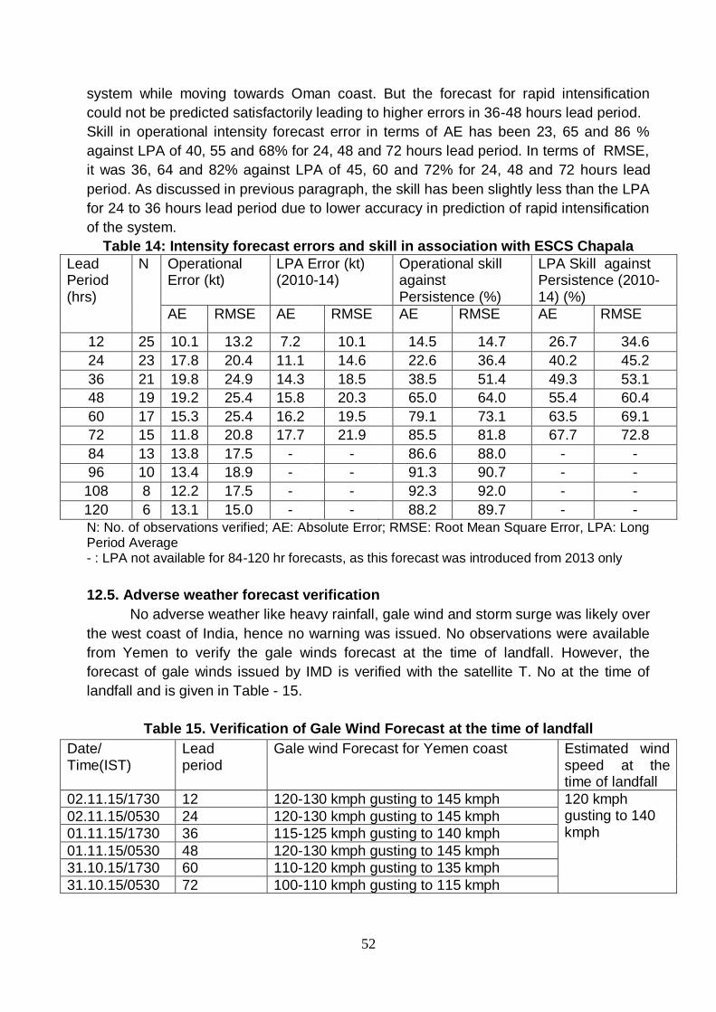
12.4. Operational Intensity forecast error and skill The operational intensity forecast errors and skill compared to persistence forecast in

terms of absolute error (AE) and root mean square error (RMSE) are presented in Table

14 . The operational AE in intensity forecast has been about 18, 19 and 12 knot against

LPA of 11, 16 and 18 knot for 24, 48 and 72 hours lead period. The forecast error has

been slightly higher than LPA for 24 and 48 hours and less for 72 hours lead period.

Similarly, operational RMSE in intensity forecast has been about 20, 25 and 21 knot

against LPA of 15, 20 and 22 knot for 24, 48 and 72 hours lead period respectively.

Slightly higher errors in 24 and 48 hours lead period is mainly attributed to rapid

intensification of the system on 29th & 30th November, which could not be predicted

operationally as well as by the numerical models. The Rapid Intensification (RI) index

developed by IMD could not predict the rapid intensification as seen from the table.

Considering the variation of intensity error w.r.t. the lead periods, the AE gradually

increased with increase in lead period from 12 hours (10 kt) to 48 hours (20 kt) lead

period. It then decreased gradually with increase in lead period upto 120 hours (13 kt).

Similarly, the RMSE increased from 12 hours (13 kt) to 48 hours (25 kt) and then

decreased towards 120 hours (15 kt) lead period. This is mainly due to the fact that IMD

could very well predict the trend in intensification and as well as the weakening of the

52

system while moving towards Oman coast. But the forecast for rapid intensification

could not be predicted satisfactorily leading to higher errors in 36-48 hours lead period.

Skill in operational intensity forecast error in terms of AE has been 23, 65 and 86 %

against LPA of 40, 55 and 68% for 24, 48 and 72 hours lead period. In terms of RMSE,

it was 36, 64 and 82% against LPA of 45, 60 and 72% for 24, 48 and 72 hours lead

period. As discussed in previous paragraph, the skill has been slightly less than the LPA

for 24 to 36 hours lead period due to lower accuracy in prediction of rapid intensification

of the system.

Table 14: Intensity forecast errors and skill in association with ESCS Chapala

Lead Period (hrs)

N Operational Error (kt)

LPA Error (kt) (2010-14)

Operational skill against Persistence (%)

LPA Skill against Persistence (2010-14) (%)

AE RMSE AE RMSE RMS AE RMSE AE RMSE

12 25 10.1 13.2 7.2 10.1 14.5 14.7 26.7 34.6

24 23 17.8 20.4 11.1 14.6 22.6 36.4 40.2 45.2

36 21 19.8 24.9 14.3 18.5 38.5 51.4 49.3 53.1

48 19 19.2 25.4 15.8 20.3 65.0 64.0 55.4 60.4

60 17 15.3 25.4 16.2 19.5 79.1 73.1 63.5 69.1

72 15 11.8 20.8 17.7 21.9 85.5 81.8 67.7 72.8

84 13 13.8 17.5 - - 86.6 88.0 - -

96 10 13.4 18.9 - - 91.3 90.7 - -

108 8 12.2 17.5 - - 92.3 92.0 - -

120 6 13.1 15.0 - - 88.2 89.7 - -

N: No. of observations verified; AE: Absolute Error; RMSE: Root Mean Square Error, LPA: Long Period Average - : LPA not available for 84-120 hr forecasts, as this forecast was introduced from 2013 only

12.5. Adverse weather forecast verification

No adverse weather like heavy rainfall, gale wind and storm surge was likely over

the west coast of India, hence no warning was issued. No observations were available

from Yemen to verify the gale winds forecast at the time of landfall. However, the

forecast of gale winds issued by IMD is verified with the satellite T. No at the time of

landfall and is given in Table - 15.

Table 15. Verification of Gale Wind Forecast at the time of landfall

Date/ Time(IST)

Lead period

Gale wind Forecast for Yemen coast Estimated wind speed at the time of landfall

02.11.15/1730 12 120-130 kmph gusting to 145 kmph 120 kmph gusting to 140 kmph

02.11.15/0530 24 120-130 kmph gusting to 145 kmph





53

13. Summary and Conclusion: The ESCS Chapala formed from a low pressure area over southeast and

adjoining southwest and eastcentral Arabian Sea on 26th Nov which concentrated into a

depression in the morning of 28th October. The system underwent rapid intensification

reaching the peak intensity of Extremely Severe Cyclonic Storm from 29th morning to

30th afternoon. The system initially moved north-northwestwards and then nearly

westwards and crossed Yemen coast near lat. 14.1°N and long. 48.65°E during 0100

and 0200 UTC of 3rd November.

IMD utilised all its resources to monitor and predict the genesis, track and

intensification of ESCS Chapala. The forecast of its genesis (formation of Depression)

on 28th Nov., its track, intensity, point & time of landfall, were predicted well with

sufficient lead time (3 days in advance). The forecast of track and intensity of the

system was mainly dependent on the satellite observations due to the sparse

observations over the sea over which the system traversed. The NWP models guidance

diverged w.r.t. track and intensity and especially landfall over Yemen. The SCIP model

and RI model could not capture the rapid intensification of the system may be because

both these models consider external dynamical features/ environmental parameters and

do not consider the internal dynamics of the system. Though HWRF model performance

was better in predicting the intensification of the system, but since the model is made

operational only in 2015, the confidence in its performance was less.

Compared to Long Period Average (LPA), the errors in track, intensity and

landfall point & time were higher as the error in the NWP model guidance was higher.

This is mainly because of limited data availability along the coast of Arabia and Africa

which are ingested in NWP models.

For 24 hr lead period, the operational landfall point & time error was 123 km &

+4.5hrs, track forecast error was 79 km and intensity forecast error based on absolute

error was 17.8 kts.

Following lessons were learnt on the monitoring and prediction of the system:

There is a need of observation along the coast of Arabia and Africa.

Deployment of more buoys on Arabian Sea.

To study the internal dynamics of the system, it is necessary to have

observations from the inner core of the cyclone which can be obtained

with possible manned/unmanned aircraft reconnaissance or through

remote sensing.

Development of high resolution ocean atmospheric coupled model with

better data assimilation.

14. Acknowledgements:

RSMC New Delhi duly acknowledges the contribution of the valuable inputs and

guidance from NCMRWF, IIT Bhubaneswar and NIOT Chennai. The inputs from NWP

Division, Satellite Division at IMD HQ New Delhi and Area Cyclone Warning Centre

(ACWC), Mumbai & ACWC Chennai and Cyclone Warning Centre (CWC), Ahmedabad

are also appreciated for their timely inputs required for compilation of this report.

Cyclone Warning Division India Meteorological Department ... · Arabian Sea during 28 October-04...

Documents

Transcript of Cyclone Warning Division India Meteorological Department ... · Arabian Sea during 28 October-04...