Cyber Epidemic Models with Dependencesshxu/socs/UINM_A_902407-author-proof.pdfXu et al.: Cyber...
37
Internet Mathematics Vol. 11: 76–112 Cyber Epidemic Models with Dependences Maochao Xu, Gaofeng Da, and Shouhuai Xu Abstract. Studying models of cyber epidemics over arbitrary complex networks can deepen our understanding of cyber security from a whole-system perspective. In this work, we initiate the investigation of cyber epidemic models that accommodate the dependences between the cyber attack events. Due to the notorious difficulty in deal- ing with such dependences, essentially all existing cyber epidemic models have disre- garded them. Specifically, we introduce the idea of copulas into cyber epidemic models for accommodating the dependences between the cyber attack events. We investigate the epidemic equilibrium thresholds as well as the bounds for both equilibrium and nonequilibrium infection probabilities. We further characterize the side effects of dis- regarding the due dependences between the cyber attack events by showing that the results thereof are unnecessarily restrictive or even incorrect. 1. Introduction Cyberspace (or the Internet) is perhaps the most complex man-made system. Although cyberspace has become an indispensable part of the society, economy, and national security, cyber attacks also have become an increasingly devastating problem. Despite studies and progresses in the past decades, our understanding of cyber security from a whole-system perspective, rather than from a component or building-block perspective, is still at its infant stage. This is caused by many C Taylor & Francis Group, LLC 76 ISSN: 1542-7951 print
Transcript of Cyber Epidemic Models with Dependencesshxu/socs/UINM_A_902407-author-proof.pdfXu et al.: Cyber...
Internet Mathematics Vol. 11: 76–112
Cyber Epidemic Models withDependencesMaochao Xu, Gaofeng Da, and Shouhuai Xu
Abstract. Studying models of cyber epidemics over arbitrary complex networks candeepen our understanding of cyber security from a whole-system perspective. In thiswork, we initiate the investigation of cyber epidemic models that accommodate thedependences between the cyber attack events. Due to the notorious difficulty in deal-ing with such dependences, essentially all existing cyber epidemic models have disre-garded them. Specifically, we introduce the idea of copulas into cyber epidemic modelsfor accommodating the dependences between the cyber attack events. We investigatethe epidemic equilibrium thresholds as well as the bounds for both equilibrium andnonequilibrium infection probabilities. We further characterize the side effects of dis-regarding the due dependences between the cyber attack events by showing that theresults thereof are unnecessarily restrictive or even incorrect.
1. Introduction
Cyberspace (or the Internet) is perhaps the most complex man-made system.Although cyberspace has become an indispensable part of the society, economy,and national security, cyber attacks also have become an increasingly devastatingproblem. Despite studies and progresses in the past decades, our understandingof cyber security from a whole-system perspective, rather than from a componentor building-block perspective, is still at its infant stage. This is caused by many
C© Taylor & Francis Group, LLC76 ISSN: 1542-7951 print
Xu et al.: Cyber Epidemic Models with Dependences 77
factors, including the dearth of powerful mathematical models that can captureand reason the interactions between the cyber attacks and the cyber defenses.
Recently, researchers have started pursuing the cyber-security value of “bio-logical epidemic-like” mathematical models. Although conceptually attractive,biological epidemic models cannot be directly used to describe cyber securitybecause there are many cyber-specific issues. One particular issue, which weinitiate its study, is the dependences between the cyber attack events. To thebest of our knowledge, these dependences have been explicitly disregarded inessentially all existing cyber epidemic models, perhaps because they are notori-ously difficult to cope with. Indeed, accommodating the dependences introducesyet another dimension of difficulty to cyber epidemic models that incorporatearbitrary complex network structures. However, the dependences are inherentbecause, for example, the events in which computers get infected are not inde-pendent of each other, and a malware may first infect some computers becausethe users visit some malicious websites and then viruses are spread over the net-work. Moreover, cyber attacks may be well coordinated by intelligent malwares,and the coordination causes positive dependences between the attack events.
1.1. Our Contributions
In this work, we initiate the systematic study of a new subfield in cyber epi-demic models, that is, understanding and characterizing the importance of thedependences between the attack events in cyber epidemic models that accom-modate arbitrary complex network structures. This is demonstrated through anontrivial generalization of the powerful push- and pull-based cyber epidemicmodel that was recently investigated in [18]. Specifically, we capture the depen-dences between the cyber attack events by incorporating the idea of copulas intocyber epidemic models. To the best of our knowledge, this is the first systematicstudy of cyber epidemic models that accommodate dependences, rather thandisregarding them. Specifically, we make two contributions.
First, we derive epidemic equilibrium thresholds, vis., sufficient conditions un-der which the epidemic spreading enters a nonnegative equilibrium (the spread-ing never dies out when there are pull-based attacks, meaning that only positiveequilibrium is relevant under this circumstance). Some of the sufficient condi-tions are less restrictive but require difficult-to-obtain information (i.e., theseconditions are theoretically more interesting), and the others are more restric-tive but require easy-to-obtain information (i.e., these conditions are practicallymore useful). We also derive bounds for the equilibrium infection probabili-ties and discuss their tightness. The bounds are easy to obtain/compute, andare useful especially when it is infeasible to obtain the equilibrium infection
78 Internet Mathematics
probabilities numerically (let alone analytically). For example, the upper boundscan be treated as the worst-case scenarios when provisioning defense resources.For Erdos-Renyi (ER) and power-law networks, we further propose to approxi-mate the equilibrium infection probabilities by taking advantage of the bounds.The approximation results are smaller than the upper bounds and would notunderestimate the number of infected nodes, meaning that the approximationresults can lead to more cost-effective defense. We further present bounds fornonequilibrium infection probabilities, regardless of whether the spreading con-verges to equilibrium. All the results are obtained by explicitly accommodatingthe dependence structures between the cyber attack events.
Second, we characterize the sideeffects of disregarding the due dependenceson the bounds for equilibrium infection probabilities, on the epidemic equilib-rium thresholds, and on the nonequilibrium infection probabilities. We show thatdisregarding the due dependences can make the results thereof unnecessarily re-strictive or even incorrect. We further discuss the cyber security implications ofthe side effects.
It is worth mentioning that as a first step towards ultimately tackling the de-pendence problem in cyber epidemic models, the copulas technique, which weuse in the present study, is appealing because of the following. On one hand,it leads to tractable models, while capable of coping with high-dimensional de-pendence (i.e., dependence between a large vector of random variables). On theother hand, there are families of copula structures that have been extensivelyinvestigated in the literature of Applied Probability Theory and Risk Manage-ment, and various methods have been developed for estimating the types andparameters of copula structures in practice. Of course, much research remainsto be done before we can answer questions such as: What approach is the mostappropriate for accommodating dependence in cyber epidemic models and underwhat circumstances?
1.2. Related Work
Biological epidemic models can be traced back to McKendrick and Kermack[9, 12]. In such homogeneous biological epidemic models were introduced tocomputer science for characterizing the spreading of computer viruses [8]. Het-erogeneous epidemic models, especially the ones that accommodate arbitrarynetwork structures, were not studied until recently [1, 5, 16]. These studies ledto the full-fledged push- and pull-based cyber epidemic model [18], which is thestarting point of the present study. To the best of our knowledge, all existingcyber epidemic models, which aim to accommodate arbitrary network structures(including other recent studies such as [10, 15, 19] and the references therein),
Xu et al.: Cyber Epidemic Models with Dependences 79
assumed that the attacks are independent of each other. This is plausible becauseaccommodating arbitrary network structures in cyber epidemic models alreadymake the resulting models difficult to analyze, and accommodating dependencesintroduces, as we show in the present article, another dimension of difficulty tothe models.
The only exception is due to our recent study [17], which is based on a differentapproach to modeling cyber epidemics [10]. The main contribution of [17] is toget rid of the exponential distribution assumptions for certain random variables.Moreover, the model in [17] can accommodate only the specific Marshall–Olkindependence structure between the attack events. In contrast, we here accommo-date arbitrary dependence structures between the attack events, while investi-gating the epidemic equilibrium thresholds, the equilibrium and nonequilibriuminfection probabilities, and the side effects of disregarding the due dependences.Many of these issues are not studied in the context of [17] because its focus isdifferent. This explains why the present study is the first systematic treatmentof dependences in cyber epidemic models.
The dependence modeled in the present paper is static (i.e., time invariant).This study inspired [4], which makes a further step towards modeling dynamicdependence between cyber attacks, but uses a different modeling approach.
The rest of the article is organized as follows. In Section 2 we briefly re-view some facts about copulas. In Section 3 we investigate the generalized cyberepidemic model that accommodates the dependences between the cyber attackevents. In Section 4 we characterize the side effects caused by disregarding thedue dependences. In Section 5, we conclude the article with future research prob-lems.
The following table summarizes the main notations used in this article.
G = (V,E) = the graph/network in which cyber epidemics occur, where V
is the node set and E is the edge setdeg(v) = the degree of node v in graph G = (V,E), which can be rep-
resented by adjacency matrix AIv (t), Iv ,j (t) = the state of node v at time t: Iv (t) = 1 means infected and 0
means secure; Iv ,j (t) is the state of the jth neighbor of node v(1 means infected and 0 means secure), where 1 ≤ j ≤ deg(v)
iv (t) = the probability that node v ∈ V is infected at time tiv ,j (t) = the condition probability that at time t node v ∈ V is secure
but the jth neighbor of node v is infectedi−v , i
+v = lower and upper bounds for the nonequilibrium infection
probability limt→∞ iv (t), where the system does not convergeto any equilibrium
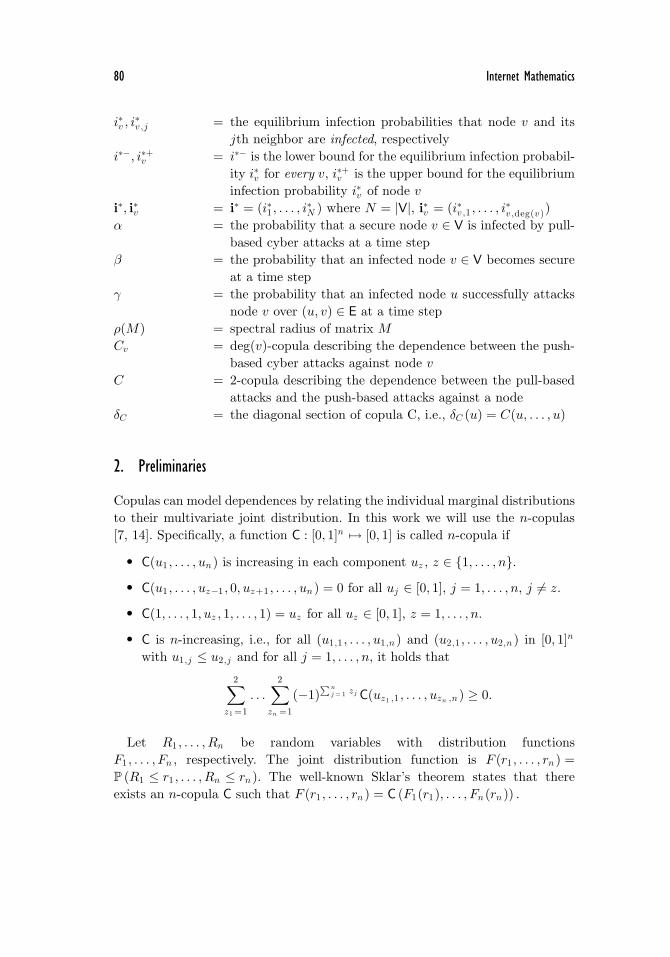
80 Internet Mathematics
i∗v , i∗v ,j = the equilibrium infection probabilities that node v and its
jth neighbor are infected, respectivelyi∗−, i∗+v = i∗− is the lower bound for the equilibrium infection probabil-
ity i∗v for every v, i∗+v is the upper bound for the equilibriuminfection probability i∗v of node v
i∗, i∗v = i∗ = (i∗1 , . . . , i∗N ) where N = |V|, i∗v = (i∗v ,1 , . . . , i
∗v ,deg(v ))
α = the probability that a secure node v ∈ V is infected by pull-based cyber attacks at a time step
β = the probability that an infected node v ∈ V becomes secureat a time step
γ = the probability that an infected node u successfully attacksnode v over (u, v) ∈ E at a time step
ρ(M) = spectral radius of matrix MCv = deg(v)-copula describing the dependence between the push-
based cyber attacks against node vC = 2-copula describing the dependence between the pull-based
attacks and the push-based attacks against a nodeδC = the diagonal section of copula C, i.e., δC (u) = C(u, . . . , u)
2. Preliminaries
Copulas can model dependences by relating the individual marginal distributionsto their multivariate joint distribution. In this work we will use the n-copulas[7, 14]. Specifically, a function C : [0, 1]n �→ [0, 1] is called n-copula if
� C(u1 , . . . , un ) is increasing in each component uz , z ∈ {1, . . . , n}.� C(u1 , . . . , uz−1 , 0, uz+1 , . . . , un ) = 0 for all uj ∈ [0, 1], j = 1, . . . , n, j �= z.
� C(1, . . . , 1, uz , 1, . . . , 1) = uz for all uz ∈ [0, 1], z = 1, . . . , n.
� C is n-increasing, i.e., for all (u1,1 , . . . , u1,n ) and (u2,1 , . . . , u2,n ) in [0, 1]n
with u1,j ≤ u2,j and for all j = 1, . . . , n, it holds that
2∑z1 =1
. . .2∑
zn =1
(−1)∑ n
j = 1 zj C(uz1 ,1 , . . . , uzn ,n ) ≥ 0.
Let R1 , . . . , Rn be random variables with distribution functionsF1 , . . . , Fn , respectively. The joint distribution function is F (r1 , . . . , rn ) =P (R1 ≤ r1 , . . . , Rn ≤ rn ). The well-known Sklar’s theorem states that thereexists an n-copula C such that F (r1 , . . . , rn ) = C (F1(r1), . . . , Fn (rn )) .
Xu et al.: Cyber Epidemic Models with Dependences 81
There are many families of copulas [7, 14]. One example is the Gaussian copulawith
C(u1 , . . . , un ) = Φ∑ (Φ−1(u1), . . . ,Φ−1(un )
),
where Φ−1 is the inverse cumulative distribution function of the standard normaldistribution, and Φ∑ is the joint cumulative distribution function of a multivari-ate normal distribution with mean vector zero and covariance matrix equal tothe correlation matrix
∑. For simplicity, we assume that the correlation matrix
has the form
∑=
⎛⎜⎜⎜⎜⎝1 σ . . . σ
σ 1 σ σ
. . .
σ σ . . . 1
⎞⎟⎟⎟⎟⎠ ,
where σ measures the correlation between two random variables. Therefore, theGaussian copula can be rewritten as
C(u1 , . . . , un ) = Φσ
(Φ−1(u1), . . . ,Φ−1(un )
).
Another example is the Archimedean family with
C(u1 , . . . , un ) = φ−1(φ(u1) + · · · + φ(un )),
where function φ is called a generator of C and satisfies certain properties (see [13]for details). The Archimedean family contains many well-known copula functionssuch as the Clayton and Frank copulas [2, 14]. The generator of the Claytoncopula is φθ (u) = u−θ − 1, and we have
C(u1 , . . . , un ) =
⎡⎣ n∑j=1
u−θj − n+ 1
⎤⎦−1/θ
, θ > 0.
The generator of the Frank copula is ψξ (u) = log( e−ξ u −1e−ξ −1 ), and we have
C(u1 , . . . , un ) = −1ξ
log
{1 +
∏nj=1(e
−ξuj − 1)(e−ξ − 1)n−1
}, ξ > 0.
For illustration purpose, we will use the Gaussian, Clayton, and Frank copulasas examples.
In order to compare the effects of dependences, we need to compare the de-grees of dependences. For this purpose, we use the concordance order [7, 14].Let C1 and C2 be two copulas; we say C1 is less than C2 in concordance orderif C1(u1 , . . . , un ) ≤ C2(u1 , . . . , un ) for all 0 ≤ ui ≤ 1, i = 1, . . . , n. In particular,
82 Internet Mathematics
Gaussian copulas and Clayton copulas are increasing in σ and θ in concordanceorder, respectively.
The following lemmas will be used in the study.
Lemma 2.1. ([14]) Let C be any n-copula, then
max
⎧⎨⎩n∑j=1
uj − n+ 1, 0
⎫⎬⎭ ≤ C(u1 , . . . , un ) ≤ min{u1 , . . . , un}.
Lemma 2.2. ([14]) Let C be an n-copula, then
|C(u1 , . . . , un ) − C(v1 , . . . , vn )| ≤n∑j=1
|uj − vj |.
3. Cyber Epidemic Model with Arbitrary Dependences
Now we present and investigate the cyber epidemic model that accommodatesthe dependences between the cyber attack events. This is the first systematictreatment of dependences in cyber epidemic models.
3.1. The Model
As in [18], we consider an undirected finite network graph G = (V,E), where V ={1, 2, . . . , N} is the set of N = |V| nodes (vertices) that can abstract computers(or software components at an appropriate resolution), and E = {(u, v) : u, v ∈V} is the set of edges. Note that G abstracts the network structure according towhich the push-based cyber attacks take place (e.g., malware spreading), where(u, v) ∈ E abstracts that node u can attack node v. In both principle and practice,G can range from a complete graph (i.e., any u ∈ V can directly attack any v ∈ V)to any specific graph structure (i.e., node u may not be able to attack node vdirectly because, for example, the traffic from node u is filtered or u is blacklistedby v), which explains why we should pursue general results without restrictingthe network/graph structures. Denote by A = (avu ) the adjacency matrix of G,where avu = 1 if and only if (u, v) ∈ E, and avu = 0, otherwise. Note that theproblem setting naturally implies avv = 0. Denote by deg(v) the degree of node v.In a discrete-time model, node v ∈ V is either secure (but vulnerable to attacks)or infected (and can attack other nodes) at any time t = 0, 1, . . .. At each timestep, an infected node v becomes secure with probability β, which abstracts
Xu et al.: Cyber Epidemic Models with Dependences 83
the defense power. The model accommodates two large classes of cyber attacks:a secure node v can become infected because of (1) pull-based cyber attackswith probability α, which include drive-by-download attacks (i.e., node v gettinginfected because its user visits a malicious website) and insider attacks (i.e., theuser intentionally runs a malware on node v), or (2) push-based cyber attackslaunched by v’s infected neighbor u over edge (u, v) ∈ E with probability γ.
Our extension to the above model is to accommodate the dependences be-tween the push-based attacks as well as the dependences between the push-basedattacks and the pull-based attacks. These attacks are not independent becausethe events that infect the nodes are not independent of each other, and becausethe push-based attacks are not independent of the pull-based attacks (e.g., amalware could first infect some nodes via the pull-based cyber attacks and thenlaunch the push-based cyber attacks from the infected nodes). Moreover, the de-pendences between the push-based attacks can model that intelligent malwareslaunch coordinated attacks against the secure nodes.
Specifically, let Iv (t) denote the state of node v at time t, where Iv (t) = 1means v is infected and 0 means v is secure. Let
(Iv ,1(t), . . . , Iv ,deg(v )(t)
)denote
the state vector of node v’s neighbors at time t, where
Iv ,j (t) =
{1, the jth neighbor of node v is infected at time t,0, otherwise.
Define iv (t) = P(Iv (t) = 1) and iv ,j (t) = P(Iv ,j (t) = 1|Iv (t) = 0), where j =1, . . . ,deg(v).
Let Xv (t) = 1 denote the event that node v is infected at time t+ 1 because ofthe push-based cyber attacks, and Xv (t) = 0, otherwise. Let Xv,j (t+ 1) = 1 de-note the event that node v is infected at time t+ 1 by its jth neighbor, andXv,j (t+ 1) = 0, otherwise. Note that P(Xv,j (t+ 1) = 1|Iv (t) = 0) = γ · iv ,j (t).Since any dependence structure between Xv,1(t+ 1), . . . , Xv,deg(v )(t+ 1) alwayscan be accommodated by some copula function Cv , we have
P(Xv (t+ 1) = 0|Iv (t) = 0)= Cv (1 − P(Xv,1(t+ 1) = 1|Iv (t) = 0), . . . , 1
−P (Xv,deg(v )(t+ 1) = 1|Iv (t) = 0))
= Cv(1 − γiv,1(t), . . . , 1 − γiv,deg(v )(t)
). (3.1)
Similarly, let Yv (t+ 1) = 1 denote the event that node v is infected at time t+ 1because of the pull-based cyber attacks. Then, we have P(Yv (t+ 1) = 1|Iv (t) =0) = α. By further accommodating the dependence structure between thepush-based attacks and the pull-based attacks via some copula function C, we
84 Internet Mathematics
have
P(Iv (t+ 1) = 1|Iv (t) = 0)= 1 − P (Xv (t+ 1) = 0, Yv (t+ 1) = 0|Iv (t) = 0)= 1 − C
(Cv
(1 − γiv,1(t), . . . , 1 − γiv,deg(v )(t)
), 1 − α
). (3.2)
Note that
P(Iv (t+ 1) = 1|Iv (t) = 1) = (1 − β)iv (t). (3.3)
From (3.1), (3.2), and (3.3), we obtain the probability that node v ∈ V is infectedat time t+ 1 as
iv (t+ 1) = P(Iv (t+ 1) = 1)= P(Iv (t+ 1) = 1|Iv (t) = 1)P(Iv (t) = 1)
+P(Iv (t+ 1) = 1|Iv (t) = 0)P(Iv (t) = 0)= (1 − β) · iv (t) + P(Iv (t+ 1) = 1|Iv (t) = 0) · (1 − iv (t))= (1 − β)iv (t) +
[1 − C
(Cv
(1 − γiv,1(t), . . . , 1 − γiv,deg(v )(t)
), 1 − α
)]× (1 − iv (t)). (3.4)
We will analyze (3.4) for v ∈ V to characterize the effects of the dependencestructures C and Cv and the side effects of disregarding them. Note that forthe special case that the Xv,j ’s are independent of each other and the push-based attacks and the pull-based attacks are also independent of each other,(3.4) degenerates to the model in [18]. Note also that in order to character-ize the side effects of disregarding the dependences, we need to accommodatethe dependences at a higher level of abstraction than the model parameters αand γ. This is because the parameters are indeed relatively easier to obtain inexperiments/practice (e.g., considering a single compromised neighbor that islaunching the push-based attacks, and considering the pull-based attacks in theabsence of the push-based attacks).
3.2. Epidemic Equilibrium Threshold and Bounds for Equilibrium Infection Probabilities
The concept of epidemic equilibrium threshold [18] naturally extends the well-known concept of epidemic threshold in that the former describes the conditionunder which the epidemic spreading converges to a nonnegative equilibrium,whereas the latter traditionally describes the condition under which the epidemicspreading converges to 0 (i.e., the spreading dies out). Note that α > 0 impliesthat the spreading will never die out and that α = 0 is necessary for the spreadingto die out. Denote by i∗v the equilibrium infection probability for node v ∈ V. In
Xu et al.: Cyber Epidemic Models with Dependences 85
the equilibrium, (3.4) becomes
i∗v = (1 − β)i∗v +[1 − C
(Cv
(1 − γi∗v ,1 , . . . , 1 − γi∗v ,deg(v )
), 1 − α
)](1 − i∗v ),
v ∈ V. (3.5)
In what follows, Theorem 3.2 gives a general epidemic equilibrium threshold(i.e., sufficient condition under which the spreading enters the equilibrium), andTheorem 3.5 gives a more succinct but more restrictive sufficient condition.
Lemma 3.1. Let A be the adjacency matrix of G. If
ρ(A) <(β + α)2
γβ, (3.6)
then system (3.4) has a unique equilibrium (i∗1 , . . . , i∗N ) ∈ [0, 1]N .
Proof. For any v ∈ V, define fv (x) : [0, 1]N → [0, 1] as
fv (x) =1 − C
(Cv
(1 − γxv,1 , . . . , 1 − γxv,deg(v )
), 1 − α
)β + 1 − C
(Cv
(1 − γxv,1 , . . . , 1 − γxv,deg(v )
), 1 − α
) , v = 1, . . . , N,
where x = (x1 , . . . , xN ) ∈ [0, 1]N . Define f(·) : [0, 1]N → [0, 1]N , where f(x) =(f1(x), . . . , fN (x)). According to the Banach fixed-point theorem [6], it is suf-ficient to show that f(x) = x has a unique solution i∗; that is, we need to provethat f(·) is a contraction mapping.
Let x, y ∈ [0, 1]N . Consider the distance between them in the Euclidean norm,
||f(x) − f(y)|| =
√√√√ N∑v=1
(fv (x) − fv (y))2 =
√√√√ N∑v=1
(βΓvΔv
)2
,
where
Γv = C(Cv
(1 − γxv,1 , . . . , 1 − γxv,deg(v )
), 1 − α
)−C (
Cv(1 − γyv,1 , . . . , 1 − γyv,deg(v )
), 1 − α
),
Δv =(β + 1 − C
(Cv
(1 − γxv,1 , . . . , 1 − γxv,deg(v )
), 1 − α
))× (
β + 1 − C(Cv
(1 − γyv,1 , . . . , 1 − γyv,deg(v )
), 1 − α
)).
By Lemmas 2.1 and 2.2, it follows that
|Γv | ≤ γ
deg(v )∑k=1
|xv,k − yv,k | and Δv ≥ (β + α)2 .
86 Internet Mathematics
Therefore, we have
||f(x) − f(y)|| ≤ βγ
(β + α)2
√√√√√ N∑v=1
⎛⎝deg(v )∑k=1
|xv,k − yv,k |⎞⎠2
.
Moreover,
N∑v=1
⎛⎝deg(v )∑k=1
|xv,k − yv,k |⎞⎠2
= (|x1 − y1 |, . . . , |xN − yN |)A2(|x1 − y1 |, . . . , |xN − yN |)T≤ ||(|x1 − y1 |, . . . , |xN − yN |)||2 ||A||2= ||x − y||2 ||A||2 ,
where ||A|| denotes the operator norm of A. Since A is a symmetric matrix, wehave
||A|| = ρ(A).
From condition (3.6), it follows that
||f(x) − f(y)|| ≤ βγρ(A)(β + α)2 ||x − y|| < ||x − y||,
which means that f(·) is a contraction mapping.
Theorem 3.2. (General epidemic equilibrium threshold.) Let A be the adjacencymatrix of G and D be the diagonal matrix with the vth (1 ≤ v ≤ N) diagonalelement equal to
h(α, β, γ, i∗v
)=
∣∣C(Cv
(1 − γi∗v ,1 , . . . , 1 − γi∗v ,deg(v )
), 1 − α
) − β∣∣,
where i∗v is the equilibrium infection probability that satisfies (3.5). Let W = D +γA. If condition (3.6) holds, namely that system (3.4) has a unique equilibrium,and the spectral radius ρ(W ) < 1, then limt→∞ iv (t) = i∗v exponentially for allv ∈ V.
Proof. According to Lemma 3.1, there is a unique solution for i∗v under condition(3.6). Denote by rv (t) = iv (t) − i∗v . We want to identify a sufficient conditionunder which limt→∞ |rv (t)| = 0 for all v ∈ V . Note that
rv (t+ 1) = rv (t)[C
(Cv
(1 − γi∗v ,1 , . . . , 1 − γi∗v ,deg(v )
), 1 − α
) − β]+
(1 − iv (t)
)×[C
(Cv
(1 − γi∗v ,1 , . . . , 1 − γi∗v ,deg(v )
), 1 − α
)−C
(Cv
(1 − γiv,1(t), . . . , 1 − γiv,deg(v )(t)
), 1 − α
)].
Xu et al.: Cyber Epidemic Models with Dependences 87
By Lemma 2.2, we have
|rv (t+ 1)| ≤ |rv (t)|h(α, β, γ, i∗v
)+ (1 − iv (t))|Cv
(1 − γi∗v ,1 , . . . , 1 − γi∗v ,deg(v )
)−Cv (1 − γiv,1(t), . . . , 1 − γiv,deg(v )(t))|
≤ |rv (t)|h(α, β, γ, i∗v
)+ γ(1 − iv (t))
deg(v )∑j=1
∣∣i∗v ,j − iv ,j (t)∣∣
≤ |rv (t)|h(α, β, γ, i∗v
)+ γ
deg(v )∑j=1
|rv,j (t)|,
where
h(α, β, γ, i∗v
)=
∣∣C(Cv
(1 − γi∗v ,1 , . . . , 1 − γi∗v ,deg(v )
), 1 − α
) − β∣∣.
Define
zv (t+ 1) = zv (t)h(α, β, γ, i∗v
)+ γ
deg(v )∑j=1
zv,j (t),
with zv (0) ≡ |rv (0)| and zv,j (0) ≡ |rv,j (0)| for j = 1, . . . ,deg(v). We see |rv (t)| ≤zv (t) for any t. Let z(t) = (z1(t), . . . , zn (t))T . Then, we have the following matrixform:
z(t+ 1) = Wz(t) = Wt+1z(0), (3.7)
whereW = D + γA, D is the diagonal matrix with diagonal element h(α, β, γ, i∗v ),and A is the adjacency matrix of G. Since matrix W is nonnegative andsymmetric, the spectral theorem [11] says that ρ(W ) is real. By using thewell-known Gelfand formula, if ρ(W ) < 1, then limt→∞Wt = 0, and therefore,limt→∞ z(t) = 0. Since
ρ(W ) = limt→∞ ‖Wt ‖1/t and ‖Wt ‖∼ [ρ(W )]t , t→ ∞,
where ‖ · ‖ is the norm in real space Rn , we conclude that ‖Wt ‖ converges
to 0 exponentially when ρ(W ) < 1. This means that the convergence rate oflimt→∞ i(t) = i∗ is at least exponential.
Use of the sufficient condition given by Theorem 3.2 requires knowing i∗ (i.e.,i∗v for all v), which is difficult to obtain analytically. It is therefore important toweaken this requirement. Now we present a sufficient condition that requires theequilibrium infection probability i∗v only for some v (rather than for all v ∈ V).According to [3], we have
ρ(W ) ≤ maxv∈V
h(α, β, γ, i∗v
)+ γρ(A).
88 Internet Mathematics
Therefore, a more restrictive sufficient condition (than that given by Theorem3.2) is to require
maxv∈V
h(α, β, γ, i∗v
)+ γρ(A) < 1, namely ρ(A) <
1 − maxv∈V h(α, β, γ, i∗v
)γ
.
According to (3.5), we have
h(α, β, γ, i∗v
)=
∣∣∣∣1 − β
1 − i∗v
∣∣∣∣ .Therefore, we obtain the following more restrictive, but more succinct, sufficientcondition:
Corollary 3.3. limt→∞ iv (t) = i∗v exponentially for all v ∈ V, if
ρ(A) ≤ min{
1 − maxv∈V |1 − β/(1 − i∗v )|γ
,(β + α)2
γβ
}. (3.8)
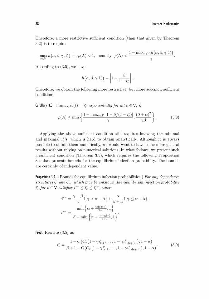
Applying the above sufficient condition still requires knowing the minimaland maximal i∗v ’s, which is hard to obtain analytically. Although it is alwayspossible to obtain them numerically, we would want to have some more generalresults without relying on numerical solutions. In what follows, we present sucha sufficient condition (Theorem 3.5), which requires the following Proposition3.4 that presents bounds for the equilibrium infection probability. The boundsare certainly of independent value.
Proposition 3.4. (Bounds for equilibrium infection probabilities.) For any dependencestructures C and Cv , which may be unknown, the equilibrium infection probabilityi∗v for v ∈ V satisfies i∗− ≤ i∗v ≤ i∗+v , where
i∗− =γ − β
γI{γ > α+ β} +
α
β + αI{γ ≤ α+ β},
i∗+v =min
{α+ γdeg(v )
β+1 , 1}
β + min{α+ γdeg(v )
β+1 , 1} .
Proof. Rewrite (3.5) as
i∗v =1 − C
(Cv
(1 − γi∗v ,1 , . . . , 1 − γi∗v ,deg(v )
), 1 − α
)β + 1 − C
(Cv
(1 − γi∗v ,1 , . . . , 1 − γi∗v ,deg(v )
), 1 − α
) . (3.9)
Xu et al.: Cyber Epidemic Models with Dependences 89
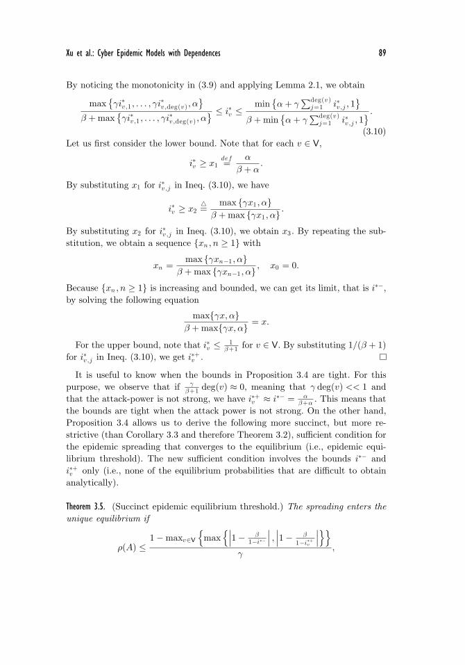
By noticing the monotonicity in (3.9) and applying Lemma 2.1, we obtain
max{γi∗v ,1 , . . . , γi
∗v ,deg(v ) , α
}β + max
{γi∗v ,1 , . . . , γi
∗v ,deg(v ) , α
} ≤ i∗v ≤ min{α+ γ
∑deg(v )j=1 i∗v ,j , 1
}β + min
{α+ γ
∑deg(v )j=1 i∗v ,j , 1
} .(3.10)
Let us first consider the lower bound. Note that for each v ∈ V,
i∗v ≥ x1def=
α
β + α.
By substituting x1 for i∗v ,j in Ineq. (3.10), we have
i∗v ≥ x2 =
max {γx1 , α}β + max {γx1 , α} .
By substituting x2 for i∗v ,j in Ineq. (3.10), we obtain x3 . By repeating the sub-stitution, we obtain a sequence {xn , n ≥ 1} with
xn =max {γxn−1 , α}
β + max {γxn−1 , α} , x0 = 0.
Because {xn , n ≥ 1} is increasing and bounded, we can get its limit, that is i∗−,by solving the following equation
max{γx, α}β + max{γx, α} = x.
For the upper bound, note that i∗v ≤ 1β+1 for v ∈ V. By substituting 1/(β + 1)
for i∗v ,j in Ineq. (3.10), we get i∗+v .
It is useful to know when the bounds in Proposition 3.4 are tight. For thispurpose, we observe that if γ
β+1 deg(v) ≈ 0, meaning that γ deg(v) << 1 andthat the attack-power is not strong, we have i∗+v ≈ i∗− = α
β+α . This means thatthe bounds are tight when the attack power is not strong. On the other hand,Proposition 3.4 allows us to derive the following more succinct, but more re-strictive (than Corollary 3.3 and therefore Theorem 3.2), sufficient condition forthe epidemic spreading that converges to the equilibrium (i.e., epidemic equi-librium threshold). The new sufficient condition involves the bounds i∗− andi∗+v only (i.e., none of the equilibrium probabilities that are difficult to obtainanalytically).
Theorem 3.5. (Succinct epidemic equilibrium threshold.) The spreading enters theunique equilibrium if
ρ(A) ≤1 − maxv∈V
{max
{∣∣∣1 − β1−i∗−
∣∣∣ , ∣∣∣1 − β
1−i∗+v
∣∣∣}}γ
,
90 Internet Mathematics
where i∗− and i∗+v are defined in Proposition 3.4.
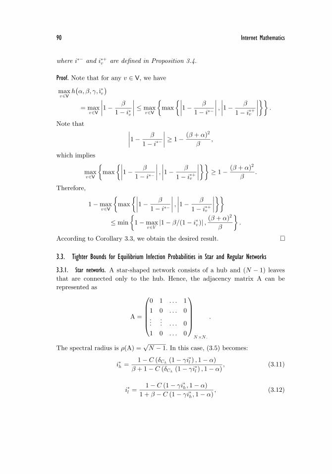
Proof. Note that for any v ∈ V, we have
maxv∈V
h(α, β, γ, i∗v
)= max
v∈V
∣∣∣∣1 − β
1 − i∗v
∣∣∣∣ ≤ maxv∈V
{max
{∣∣∣∣1 − β
1 − i∗−
∣∣∣∣ , ∣∣∣∣1 − β
1 − i∗+v
∣∣∣∣}}.
Note that ∣∣∣∣1 − β
1 − i∗−
∣∣∣∣ ≥ 1 − (β + α)2
β,
which implies
maxv∈V
{max
{∣∣∣∣1 − β
1 − i∗−
∣∣∣∣ , ∣∣∣∣1 − β
1 − i∗+v
∣∣∣∣}}≥ 1 − (β + α)2
β.
Therefore,
1 − maxv∈V
{max
{∣∣∣∣1 − β
1 − i∗−
∣∣∣∣ , ∣∣∣∣1 − β
1 − i∗+v
∣∣∣∣}}≤ min
{1 − max
v∈V|1 − β/(1 − i∗v )| ,
(β + α)2
β
}.
According to Corollary 3.3, we obtain the desired result.
3.3. Tighter Bounds for Equilibrium Infection Probabilities in Star and Regular Networks
3.3.1. Star networks. A star-shaped network consists of a hub and (N − 1) leavesthat are connected only to the hub. Hence, the adjacency matrix A can berepresented as
A =
⎛⎜⎜⎜⎜⎝0 1 . . . 11 0 . . . 0...
... . . . 01 0 . . . 0
⎞⎟⎟⎟⎟⎠N×N.
.
The spectral radius is ρ(A) =√N − 1. In this case, (3.5) becomes:
i∗h =1 − C (δCh
(1 − γi∗l ) , 1 − α)β + 1 − C (δCh
(1 − γi∗l ) , 1 − α), (3.11)
i∗l =1 − C (1 − γi∗h , 1 − α)
1 + β − C (1 − γi∗h , 1 − α), (3.12)
Xu et al.: Cyber Epidemic Models with Dependences 91
where i∗h and i∗l are the equilibrium probabilities that the hub and the leaves areinfected, respectively. Note that the effect of the copula Ch on the equilibriumprobabilities depends only on its diagonal section δCh
.In what follows, we present two results about the equilibrium infection proba-
bilities, which are not implied by the above general results that apply to arbitrarynetwork structures. First, we can prove i∗h ≥ i∗l .
Proposition 3.6. For the star networks, it holds that i∗h ≥ i∗l .
Proof. Denote by
f(x) =1 − C (δCh
(1 − γx) , 1 − α)β + 1 − C (δCh
(1 − γx) , 1 − α)and g(x) =
1 − C (1 − γx, 1 − α)1 + β − C (1 − γx, 1 − α)
where x ∈ [0, 1]. Since δCh(x) ≤ x, we have f(x) ≥ g(x). Suppose i∗h < i∗l and
(i∗h , i∗l ) is a solution to (3.11) and (3.12). Then, i∗h = f(i∗l ) = g−1(i∗l ) < i∗l . Since
g(x) is increasing in x and so is g−1 , we have i∗l ≤ g(i∗l ) and f(i∗l ) < i∗l ≤ g(i∗l ),which contradicts f(x) ≥ g(x) for x ∈ [0, 1].
Second, we present refined bounds for equilibrium infection probabilities i∗hand i∗l . The bounds are useful because even in the case of star networks, it isdifficult to derive analytic expressions and infeasible to numerically compute(especially for complex dependence structures) i∗h and i∗l .
Proposition 3.7. (Tighter upper bounds for the equilibrium infection probabilitiesin star networks.) For star networks and regardless of the dependence structures(which can be unknown), we have i∗− ≤ i∗h ≤ i∗+h and i∗− ≤ i∗l ≤ i∗+l , wherei∗− is defined in Proposition 3.4 and
i∗+h =1
β + 1I{
1β + 1
≥ 1 − α
(N − 1)γ
}+
(N − 1)γ − α− β +√
((N − 1)γ − α− β)2 + 4(N − 1)γα2(N − 1)γ
× I{
1β + 1
<1 − α
(N − 1)γ
},
and
i∗+l =1
β + 1I{
1β + 1
≥ 1 − α
γ
}+γ − α− β +
√(γ − α− β)2 + 4γα2γ
× I{
1β + 1
<1 − α
γ
}.
92 Internet Mathematics
Proof. The lower bound i∗− is the same as that in Proposition 3.4. Let’s focus oni∗+h . From Ineq. (3.10), we have
i∗h ≤ min{α+ (N − 1)γi∗l , 1}β + min{α+ (N − 1)γi∗l , 1}
= f(i∗l ).
Because the right-hand side of the above inequality increases in i∗l , by Proposition3.6 we have
i∗h ≤ f(i∗h
),
and therefore, i∗h ≤ i∗+h , where i∗+h is the solution to equation
x = f(x). (3.13)
For the upper bound i∗+l , we can similarly obtain the desired result by solvingequation
x = f
(x
N − 1
). (3.14)
Now we explain why the upper bounds i∗+h and i∗+l given by Proposition3.7 are smaller (i.e., tighter) than the general upper bounds that can be de-rived from Proposition 3.4 by instantiating G = (V,E) as star networks. Tosee this, we note that i∗+h is the solution to (3.13) and i∗+h ≤ 1
β+1 , meaningthat
i∗+h ≤min
{α+ (N − 1) γ
β+1 , 1}
β + min{α+ (N − 1) γ
β+1 , 1} ,
where the right-hand side of the inequality is exactly the upper bound that canbe derived from Proposition 3.4 by substituting deg(v) with the degree of thehub. This means that i∗+h is smaller than the upper bound given by Proposition3.4. Similarly, we can show that i∗+l is smaller than the upper bound given byProposition 3.4. Moreover, by comparing (3.13) and (3.14), we see that i∗+h ≥ i∗+l .Because the lower bound i∗− is the same as the lower bound given by Proposition3.4, we conclude that the bounds given by Proposition 3.7 are tighter than thebounds given by Proposition 3.4.
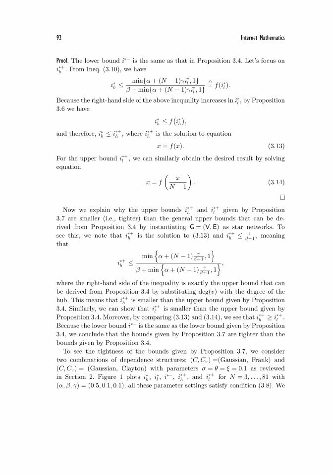
To see the tightness of the bounds given by Proposition 3.7, we considertwo combinations of dependence structures: (C,Cv ) =(Gaussian, Frank) and(C,Cv ) = (Gaussian, Clayton) with parameters σ = θ = ξ = 0.1 as reviewedin Section 2. Figure 1 plots i∗h , i
∗l , i
∗−, i∗+h , and i∗+l for N = 3, . . . , 81 with(α, β, γ) = (0.5, 0.1, 0.1); all these parameter settings satisfy condition (3.8). We
Xu et al.: Cyber Epidemic Models with Dependences 93
0 20 40 60 80
0.75
0.80
0.85
0.90
0.95
Star
Leaves
upper boundnumerical solutionlower bound
(a) Hub: (Gaussian, Frank)
0 20 40 60 80
0.83
0.84
0.85
0.86
0.87
Star
Leaves
upper boundnumerical solutionlower bound
(b) Leaves: (Gaussian, Frank)
0 20 40 60 80
0.75
0.80
0.85
0.90
0.95
Star
Leaves
upper boundnumerical solutionlower bound
(c) Hub: (Gaussian, Clayton)
0 20 40 60 80
0.83
0.84
0.85
0.86
0.87
Star
Leaves
upper boundnumerical solutionlower bound
(d) Leaves: (Gaussian, Clayton)Figure 1. Star networks: upper bound i∗+h for hub (i∗+l for leaves) vs. numericalsolution i∗h for hub (i∗l for leaves) vs. lower bound i∗− (for both hub and leaves)with respect to (α, β, γ) = (0.5, 0.1, 0.1) and (C,Cv ).
observe that the upper bound i∗+h becomes flat for N ≥ 5, because it causesi∗+h = 1
β+1 (i.e., independent of N); whereas, the upper bound i∗+l is flat becauseit is always independent of N . We observe that the upper bound for hub node,i∗+h , becomes extremely tight for dense star networks with N > 40. However, theupper bound for leaf nodes almost always exhibits that i∗+l − i∗l ≈ 0.011 (i.e.,the upper bound overestimates about 0.88 infected nodes for a star network ofN = 80 nodes). In any case, the upper bounds only somewhat overestimate thenumerical solutions i∗v ’s and thus can be used for decision-making purpose wheni∗v ’s are infeasible to compute.
94 Internet Mathematics
3.3.2. Regular Networks. For regular networks, each node v ∈ V has degree d for somed ∈ [1, N − 1] and ρ(A) = d. According to Proposition 3.4, we have
i∗v =1 − C
(Cv
(1 − γi∗v ,1 , . . . , 1 − γi∗v ,d
), 1 − α
)β + 1 − C
(Cv
(1 − γi∗v ,1 , . . . , 1 − γi∗v ,d
), 1 − α
) , v ∈ V.
Now we want to present refined bounds for equilibrium infection probability i∗v .
Proposition 3.8. (Tighter upper bound for the equilibrium infection probability inregular networks.) For regular network G = (V,E) and regardless of the depen-dence structures (which can be unknown), we have i∗− ≤ i∗v ≤ i∗+ for any v ∈ V,where i∗− is defined in Proposition 3.4 and
i∗+ =1
β + 1I{
1β + 1
≥ 1 − α
γd
}+γd− α− β +
√(γd− α− β)2 + 4γαd2γd
× I{
1β + 1
<1 − α
γd
}.
Proof. Define function
f(x) =min{α+ γdx, 1}
β + min{α+ γdx, 1}and a sequence {xn , n ≥ 0} with xn = f(xn−1), x0 = 1/(β + 1). Observe that forall v ∈ V, we have i∗v ≤ x0 and hence from Ineq. (3.10), it follows that i∗v ≤ x1
for all v ∈ V. By repeating this process, we have i∗v ≤ xn for all n. Since f(x) isincreasing and x1 ≤ x0 , xn is decreasing in n. Thus, we have i∗v ≤ i∗+, which isthe solution of the equation x = f(x). If 1
β+1 ≥ 1−αγd , then i∗+ = 1
β+1 ; otherwise,i∗+ is the positive solution to equation γdx2 + (α+ β − γd)x− α = 0. Thus, weobtain the desired result.
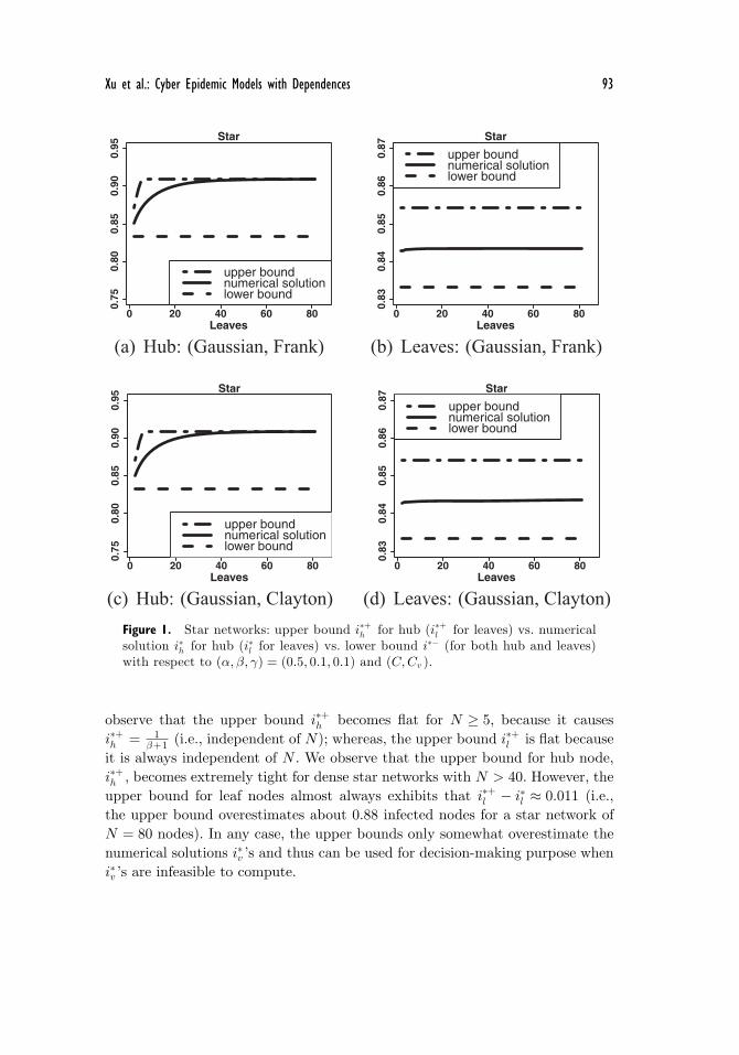
Note that the upper bound i∗+ given by Proposition 3.8 is smaller than theupper bound i∗+v obtained by instantiating deg(v) = d in Proposition 3.4, be-cause i∗+v is exactly the x1 defined in the proof of Proposition 3.8. To seethe tightness of bounds i∗− and i∗+ given by Proposition 3.8, we consider(C,Cv ) =(Gaussian, Frank) and (C,Cv ) =(Gaussian, Clayton) with parametersσ = θ = ξ = 0.1 as reviewed in Section 2. Figure 2 plots numerical i∗v , i
∗− andi∗+ with respect to node degree d = 2, . . . , 80 with (α, β, γ) = (0.5, 0.1, 0.01);all these parameter settings satisfy condition (3.8). We observe that i∗+v be-comes flat for sufficiently dense regular networks. This is because i∗+v = 1
β+1
when d ≥ (1−α)(β+1)γ . For (C,Cv ) =(Gaussian, Frank), we further observe that
the upper bound i∗+v is reasonably tight, especially for relatively sparse regu-lar networks, with i∗+v − i∗v < 0.021 for d < 20 (i.e., for a sparse regular network
Xu et al.: Cyber Epidemic Models with Dependences 95
0 20 40 60 80
0.80
0.85
0.90
0.95
1.00
Regular
Degree
upper boundnumerical solutionlower bound
(a) (Gaussian, Frank,0.5,0.1,0.01)
0 20 40 60 80
0.80
0.85
0.90
0.95
1.00
Regular
Degree
upper boundnumerical solutionlower bound
(b) (Gaussian, Clayton,0.5,0.1,0.01)
Figure 2. Regular networks: upper bound i∗+v vs. numerical solution i∗v vs. lowerbound i∗−v with respect to (C,Cv , α, β, γ).
of N = 1000 nodes, the upper bound overestimates at most only 21 infectednodes). Even for dense regular network with d > 20, we have i∗+v − i∗v ≤ 0.038(i.e., for a dense regular network of N = 1000 nodes, the upper bound over-estimates at most only 38 infected nodes), where equality holds for d = 54. For(C,Cv ) =(Gaussian, Clayton), we also observe that the upper bound i∗+v is tight,especially for relatively sparse regular networks with d < 20 and i∗+v − i∗v < 0.021(i.e., for a sparse regular network of N = 1000 nodes, the upper bound overes-timates at most only 21 infected nodes). Even for dense regular network withd > 20, we have i∗+v − i∗v ≤ 0.039, where equality holds for d = 54. This meansthat for decision-making purpose, the defender can use the upper bound i∗+vinstead of the numerical solution i∗v , especially when i∗v is infeasible to compute.
3.4. Approximating Equilibrium Infection Probabilities in ER and Power-Law Networks
For star and regular networks, we have derived tighter bounds for equilibriuminfection probabilities (than the general bounds given by Proposition 3.4). Un-fortunately, we do not know how to derive tighter bounds for ER and power-lawnetworks. As an alternative, we propose to approximate equilibrium infectionprobabilities by taking advantage of the upper and lower bounds. The approxi-mation is useful because it is often smaller than the upper bound, which neverunderestimates, but may substantially overestimate, the threats in terms of equi-librium infection probabilities. That is, the approximation method can lead tomore cost-effective defense than the upper bound.
The approximation method is the following: We first compute lower bounds,upper bounds, and numerical solutions for a feasible number of instances of(G, C, Cv , α, β, γ), based on given computer resources. We then use the resultingdata to derive (via statistical methods) some function of the lower and upperbounds. For even larger G of the same type, as well as (C,Cv ) of the same kind,
96 Internet Mathematics
the resulting function would be smaller than the upper bound and would notunderestimate the equilibrium infection probabilities. The key insight is that wecan compute, for networks of any size, the upper and lower bounds according toProposition 3.4. This means that we can approximate the equilibrium infectionprobabilities for arbitrarily large networks, for which it is often infeasible to nu-merically (let alone analytically) compute the equilibrium infection probabilities.
To illustrate the approximation method, we also consider (C,Cv ) =(Gaussian,Frank) and (C,Cv ) =(Gaussian, Clayton) with parameters σ = θ = ξ = 0.1as reviewed in Section 2. We use the erdos.renyi.game generator ofthe igraph package in the R system to generate a random ER networkof N = 1000 nodes and edge probability 0.01; the resulting network in-stance has spectral radius 11.38045. We use the static.power.law.game
generator of the igraph package in the R system to generate a randompower-law network of N = 1000 nodes, 5000 edges, and power-law expo-nent 2.1 (note that 2.1 is the power-law exponent of the Internet AS-levelnetwork [5]); the resulting network instance has spectral radius 22.97582.We consider combinations of (α, β, γ) that satisfy condition (3.8), whereα ∈ {0.01, 0.05, 0.1, 0.2, 0.3, 0.4, 0.5}, β ∈ {0.1, 0.2, 0.3, 0.4, 0.5, 0.6, 0.7, 0.8, 0.9},γ ∈ {0.01, 0.02, 0.03, 0.04, 0.05, 0.06, 0.07, 0.08, 0.09, 0.1}. It turns out that for(C,Cv ) =(Gaussian, Frank), the ER network has 307 combinations of (α, β, γ)that satisfy condition (3.8); the power-law network has 125 combinations of(α, β, γ) that satisfy condition (3.8), because the spectral radius is larger. For(C,Cv ) =(Gaussian, Clayton), the ER network has 307 combinations of (α, β, γ)that satisfy condition (3.8); the power-law network has 126 combinations of(α, β, γ) that satisfy condition (3.8).
We compute equilibrium infection probability i∗v numerically by solving (3.5)for v ∈ V via the BB package in the R system. We compute the upper and lowerbounds, namely i∗− and i∗+v , according to Proposition 3.4. Because it is infeasibleto numerically compute i∗v for large networks, we propose to approximate i∗v fornode v ∈ V via i∗v = 1
2 (i∗v + i∗+v ), where
i∗v = f(C,Cv )(i∗−, i∗+v ,deg(v)
)= k0 + k1i
∗− + k2i∗+v + k3 deg(v)
can be statistically derived from the data. Note that the heuristic function i∗vcould be refined via more extensive numerical studies. We define the approxi-mation error for network G as errG =
∑v∈V(i∗v − i∗v ), because
∑v∈V i
∗v is an im-
portant factor for cyber defense decision-making. For practical use, it is desiredthat errG ≥ 0, meaning that the defender never underestimates the threats, andat the same time, errG ≈ 0, meaning that the defender does not overestimate thethreats (i.e., does not overprovision defense resources) too much.
Xu et al.: Cyber Epidemic Models with Dependences 97
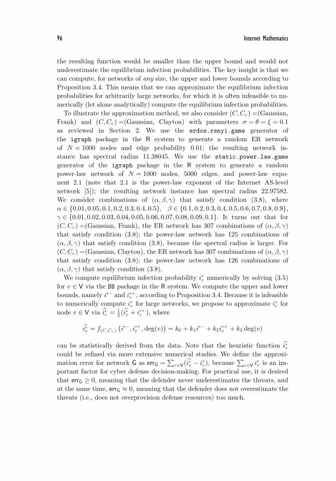
3.4.1. ER networks. For the ER network, we obtain the following formulas :
� For (C,Cv ) = (Gaussian, Frank), we have i∗v = −0.01759 + 0.3142i∗− +0.7294i∗+v − 0.0002575 deg(v).
� For (C,Cv ) = (Gaussian, Clayton), we have i∗v = −0.0174076 +0.3150585i∗− + 0.7281992i∗+v − 0.0002596 deg(v).
For (C,Cv ) = (Gaussian, Frank), the average of the errG’s over the 307 combi-nations of (C,Cv , α, β, γ) is 46, meaning that the approximation method overes-timates only 46 infected nodes in an ER network of 1000 nodes. In comparison,the average of the
∑v∈V(i∗+v − i∗v )’s over the 307 combinations of (C,Cv , α, β, γ)
is 93, meaning that the upper bound overestimates 93 infected nodes (i.e., theapproximation method is indeed better); the average of the
∑v∈V(i− − i∗v )’s is
−52.7, meaning that the lower bound underestimates 52.7 infected nodes in anER network of 1000 nodes. Finally, we note that among the 307 combinationsof (C,Cv , α, β, γ), the maximum errG is 165.2, which is elaborated in Figure 3(a)and will be discussed further, and the minimum errG is 4.1, which is elaboratedin Figure 3(b) and will be discussed further as well. For (C,Cv ) =(Gaussian,Clayton), the average of the errG’s over the 307 combinations of (C,Cv , α, β, γ)is 46.5, meaning that the approximation method only overestimates 46.5 in-fected nodes in an ER network of 1000 nodes. In comparison, the average ofthe
∑v∈V(i∗+v − i∗v )’s over the 307 combinations of (C,Cv , α, β, γ) is 93, mean-
ing that the upper bound overestimates 93 infected nodes in an ER networkof 1000 nodes; the average of the 307
∑v∈V(i− − i∗v )’s is −52.5, meaning that
the lower bound underestimates 52.5 infected nodes in an ER network of 1000nodes. Among the 307 instances, the maximum errG is 165.0, which is elaboratedin Figure 3(d) and will be discussed further, and the minimum errG is 4.2, whichis elaborated in Figure 3(e) and will be discussed further. In summary, cyber de-fense decision-making can be based on the approximation method, which takesadvantage of the upper and lower bounds and would be better (smaller) thanthe upper bound.
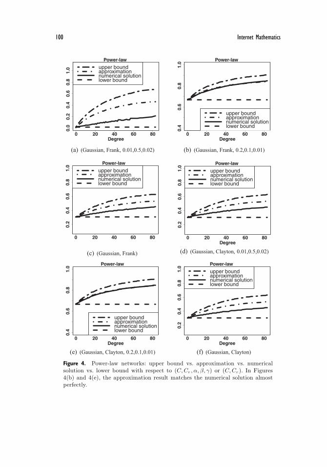
As a side product, we would like to highlight the phenomenon that the equi-librium infection probability i∗v increases with node degree deg(v). This phe-nomenon was observed in [18] in the absence of dependence, and persists in thepresence of dependence as we elaborate below. We consider i∗+v , i∗v , i∗v and i∗−
with respect to distinct node degrees, by taking the average of the nodes ofthe same degree when needed. For (C,Cv ) =(Gaussian, Frank), Figures 3(a)–3(b) plot the infection probabilities corresponding to the (α, β, γ) that leadsto the maximum and minimum errG, respectively; Figure 3(c) plots the infec-tion probabilities averaged over the 307 combinations of (α, β, γ) that satisfy
98 Internet Mathematics
5 10 15 20
0.0
0.2
0.4
0.6
0.8 ER
Degree
upper boundapproximationnumerical solutionlower bound
(a) (Gaussian, Frank, 0.01,0.4,0.03)
5 10 15 20
0.20
0.25
0.30
0.35
0.40
ER
Degree
upper boundapproximationnumerical solutionlower bound
(b) (Gaussian, Frank, 0.3,0.9,0.01)
5 10 15 20
0.2
0.4
0.6
0.8
1.0 ER
Degree
upper boundapproximationnumerical solutionlower bound
(c) (Gaussian,Frank)
5 10 15 20
0.0
0.2
0.4
0.6
0.8 ER
Degree
upper boundapproximationnumerical solutionlower bound
(d) (Gaussian, Clayton, 0.01,0.4,0.03)
5 10 15 20
0.20
0.25
0.30
0.35
0.40
ER
Degree
upper boundapproximationnumerical solutionlower bound
(e) (Gaussian, Clayton, 0.3,0.9,0.01)
5 10 15 20
0.2
0.4
0.6
0.8
1.0 ER
Degree
upper boundapproximationnumerical solutionlower bound
(f) (Gaussian,Clayton)
Figure 3. ER networks: upper bound vs. approximation vs. numerical solutionvs. lower bound with respect to (C,Cv , α, β, γ) or (C,Cv ).
Xu et al.: Cyber Epidemic Models with Dependences 99
condition (3.8). For (C,Cv ) =(Gaussian, Clayton), Figures 3(d)–3(e) plot theinfection probabilities corresponding to the (α, β, γ) that leads to the maximumand minimum errG, respectively; Figure 4(f) plots the infection probabilities av-eraged over the 307 combinations of (α, β, γ) that satisfy condition (3.8). Weobserve that the approximation i∗v can slightly underestimate the infection prob-ability i∗v for node v of degree deg(v) ≤ 5, but the overall estimation
∑v∈V i
∗v
is still above the actual threats∑
v∈V i∗v (as mentioned previous). More im-
portantly, we observe that i∗v (solid curves) increases with deg(v). This hintsthat there might be some universal scaling laws, in the presence or absenceof dependence. It is an interesting future work to identify the possible scalinglaw.
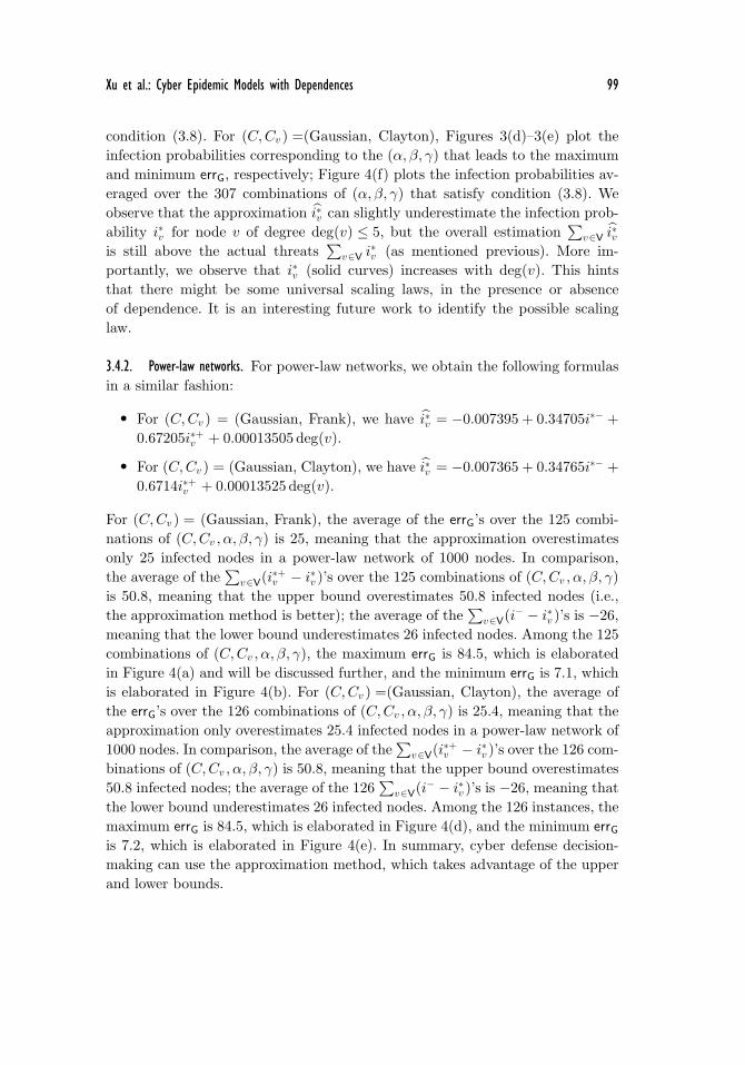
3.4.2. Power-law networks. For power-law networks, we obtain the following formulasin a similar fashion:
� For (C,Cv ) = (Gaussian, Frank), we have i∗v = −0.007395 + 0.34705i∗− +0.67205i∗+v + 0.00013505 deg(v).
� For (C,Cv ) = (Gaussian, Clayton), we have i∗v = −0.007365 + 0.34765i∗− +0.6714i∗+v + 0.00013525 deg(v).
For (C,Cv ) = (Gaussian, Frank), the average of the errG’s over the 125 combi-nations of (C,Cv , α, β, γ) is 25, meaning that the approximation overestimatesonly 25 infected nodes in a power-law network of 1000 nodes. In comparison,the average of the
∑v∈V(i∗+v − i∗v )’s over the 125 combinations of (C,Cv , α, β, γ)
is 50.8, meaning that the upper bound overestimates 50.8 infected nodes (i.e.,the approximation method is better); the average of the
∑v∈V(i− − i∗v )’s is −26,
meaning that the lower bound underestimates 26 infected nodes. Among the 125combinations of (C,Cv , α, β, γ), the maximum errG is 84.5, which is elaboratedin Figure 4(a) and will be discussed further, and the minimum errG is 7.1, whichis elaborated in Figure 4(b). For (C,Cv ) =(Gaussian, Clayton), the average ofthe errG’s over the 126 combinations of (C,Cv , α, β, γ) is 25.4, meaning that theapproximation only overestimates 25.4 infected nodes in a power-law network of1000 nodes. In comparison, the average of the
∑v∈V(i∗+v − i∗v )’s over the 126 com-
binations of (C,Cv , α, β, γ) is 50.8, meaning that the upper bound overestimates50.8 infected nodes; the average of the 126
∑v∈V(i− − i∗v )’s is −26, meaning that
the lower bound underestimates 26 infected nodes. Among the 126 instances, themaximum errG is 84.5, which is elaborated in Figure 4(d), and the minimum errGis 7.2, which is elaborated in Figure 4(e). In summary, cyber defense decision-making can use the approximation method, which takes advantage of the upperand lower bounds.
100 Internet Mathematics
0 20 40 60 80
0.0
0.2
0.4
0.6
0.8
1.0
Power-law
Degree
upper boundapproximationnumerical solutionlower bound
(a) (Gaussian, Frank, 0.01,0.5,0.02)
0 20 40 60 80
0.4
0.6
0.8
1.0 Power-law
Power-law
Power-law Power-law
Power-law
Degree
upper boundapproximationnumerical solutionlower bound
(b) (Gaussian, Frank, 0.2,0.1,0.01)
0 20 40 60 80
0.2
0.4
0.6
0.8
1.0
upper boundapproximationnumerical solutionlower bound
(c) (Gaussian, Frank)
0 20 40 60 80
0.2
0.4
0.6
0.8
1.0
Degree
upper boundapproximationnumerical solutionlower bound
(d) (Gaussian, Clayton, 0.01,0.5,0.02)
0 20 40 60 80
0.4
0.6
0.8
1.0
Degree
upper boundapproximationnumerical solutionlower bound
(e) (Gaussian, Clayton, 0.2,0.1,0.01)
0 20 40 60 80
0.2
0.4
0.6
0.8
1.0
Degree
upper boundapproximationnumerical solutionlower bound
(f) (Gaussian, Clayton)
Figure 4. Power-law networks: upper bound vs. approximation vs. numericalsolution vs. lower bound with respect to (C,Cv , α, β, γ) or (C,Cv ). In Figures4(b) and 4(e), the approximation result matches the numerical solution almostperfectly.
Xu et al.: Cyber Epidemic Models with Dependences 101
We also would like to highlight the phenomenon that the equilibrium infectionprobability i∗v increases with node degree deg(v) in power-law networks. Simi-larly, for (C,Cv ) =(Gaussian, Frank), Figures 4(a)–4(b) plot, respectively, theinfection probabilities corresponding to the (α, β, γ) that leads to the maximumand minimum errG, and Figure 4(c) plots the infection probabilities averagedover the 125 combinations of (C,Cv , α, β, γ) that satisfy condition (3.8). For(C,Cv ) =(Gaussian, Clayton), Figures 4(a)–4(b) plot respectively the infectionprobabilities corresponding to the (α, β, γ) that leads to the maximum errG, andFigure 4(c) plots the infection probabilities averaged over the 126 combinationsof (C,Cv , α, β, γ) that satisfy condition (3.8). We observe that the approxima-tion i∗v never underestimates the infection probability i∗v for any node v. Wealso observe that i∗v (solid curves) increases with deg(v), but exhibits a highernonlinearity when compared with the ER networks.
3.5. Bounds for Nonequilibrium Infection Probabilities
It is important to characterize the behavior of iv (t) even if it never enters anyequilibrium. For this purpose, we want to seek some bounds for iv (t), regardlessof whether the system converges to an equilibrium. Such characterization is usefulbecause, for example, the upper bound can be used for the worst-case scenariodecision-making. It is worth mentioning that nonequilibrium states/behaviorsare always hard to characterize.
Proposition 3.9. (Bounds for nonequilibrium probabilities.) Let limt→∞iv (t) andlimt→∞iv (t) denote the upper and lower limits of iv (t), v ∈ V. Then,
i−v ≤ limt→∞iv (t) ≤ limt→∞iv (t) ≤ i+v ,
where
i−v =
⎧⎪⎪⎨⎪⎪⎩1 − C(δCv
(1 − γν), 1 − α)β + 1 − C(δCv
(1 − γν), 1 − α) , C(δCv(1 − γν), 1 − α) ≥ β,
[β − C(δCv(1 − γν), 1 − α)] (1 − μv ) + 1 − β, otherwise,
and
i+v =
⎧⎪⎪⎪⎪⎪⎪⎪⎪⎨⎪⎪⎪⎪⎪⎪⎪⎪⎩
1 − C(Cv
(1 − γμv,1 , . . . , 1 − γμv,deg(v )
), 1 − α
)β + 1 − C
(Cv
(1 − γμv,1 , . . . , 1 − γμv,deg(v )
), 1 − α
) ,C
(Cv
(1 − γμv,1 , . . . , 1 − γμv,deg(v )
), 1 − α
)> β[
β − C(Cv
(1 − γμv,1 , . . . , 1 − γμv,deg(v )
), 1 − α
)](1 − i−v ) + 1 − β,
otherwise
102 Internet Mathematics
with δCv(1 − γν) = Cv (1 − γν, . . . , 1 − γν), μv = max{1 − β,min{γdeg(v) +
α, 1}} and ν = min{1 − β, α}.
Proof. By observing the monotonicity in (3.4), we note that iv (t) ≥ ν for all v ∈ V.Replacing iv ,j (t) with ν in (3.4) yields
iv (t+ 1) ≥ (1 − β)iv (t) + [1 − C (δCv(1 − γν), 1 − α)] (1 − iv (t))
= [C (δCv(1 − γν), 1 − α) − β] iv (t) + 1 − C (δCv
(1 − γν), 1 − α) .
If C (δCv(1 − γν), 1 − α) > β, by taking the lower limit on both sides we obtain
limt→∞iv (t+ 1) ≥ 1 − C (δCv(1 − γν), 1 − α)
β + 1 − C (δCv(1 − γν), 1 − α)
.
If C (δCv(1 − γν), 1 − α) ≤ β, we have
iv (t+ 1)≥ [C(δCv
(1 − γν), 1 − α) − β]μv + 1 − C(δCv(1 − γν), 1 − α)
= [β − C(δCv(1 − γν), 1 − α)](1 − μv ) + 1 − β.
Hence, limt→∞iv (t) ≥ i−v .For the upper bound, by applying Lemma 2.1 to (3.4) we have
iv (t+ 1)≤ (1 − β)iv (t) + [1 − max {max {2 − γdeg(v) − α, 1 − α} − 1, 0}] (1 − iv (t))= (1 − β)iv (t) + min {γdeg(v) + α, 1} (1 − iv (t))≤ max {1 − β,min{γdeg(v) + α, 1}} = μv . (3.15)
By replacing iv ,j with μv,j ’s in (3.4) yields
iv (t+ 1)≤ (1 − β)iv (t) +
[1 − C
(Cv
(1 − γμv,1 , . . . , 1 − γμv,deg(v )
), 1 − α
)](1 − iv (t))
=[C
(Cv
(1 − γμv,1 , . . . , 1 − γμv,deg(v )
), 1 − α
) − β]iv (t)
+1 − C(Cv
(1 − γμv,1 , . . . , 1 − γμv,deg(v )
), 1 − α
).
If C(Cv (1 − γμv,1 , . . . , 1 − γμv,deg(v )), 1 − α) > β, then
limt→∞ ≤ 1 − C(Cv
(1 − γμv,1 , . . . , 1 − γμv,deg(v )
), 1 − α
)β + 1 − C
(Cv
(1 − γμv,1 , . . . , 1 − γμv,deg(v )
), 1 − α
) .
Xu et al.: Cyber Epidemic Models with Dependences 103
If C(Cv (1 − γμv,1 , . . . , 1 − γμv,deg(v )), 1 − α) ≤ β, then we have
limt→∞iv (t+ 1)≤ limt→∞
{[C
(Cv
(1 − γμv,1 , . . . , 1 − γμv,deg(v )
), 1 − α
) − β]iv (t)
+1 − C(Cv
(1 − γμv,1 , . . . , 1 − γμv,deg(v )
), 1 − α
)}≤ [
C(Cv
(1 − γμv,1 , . . . , 1 − γμv,deg(v )
), 1 − α
) − β]limt→∞iv (t)
+1 − C(Cv
(1 − γμv,1 , . . . , 1 − γμv,deg(v )
), 1 − α
)≤ [
C(Cv
(1 − γμv,1 , . . . , 1 − γμv,deg(v )
), 1 − α
) − β]i−v
+1 − C(Cv
(1 − γμv,1 , . . . , 1 − γμv,deg(v )
), 1 − α
).
Hence, we have limt→∞iv (t+ 1) ≤ i+v .
3.5.1. When are the bounds tight?. It is important to know when the bounds are tightbecause the defender can use the upper bound i+v for decision-making, especiallywhen the spreading never enters any equilibrium. Note that when γ << 1, itholds that
C(δCv(1 − γν), 1 − α) ≈ C(1, 1 − α) = 1 − α,
and
C(Cv (1 − γμv,1 , . . . , 1 − γμv,deg(v )), 1 − α) ≈ C(Cv (1, . . . , 1), 1 − α) = 1 − α.
Therefore, in the case γ << 1 and α+ β < 1, we have
i−v ≈ 1 − C(δCv(1 − γν), 1 − α)
β + 1 − C(δCv(1 − γν), 1 − α)
≈ α
β + α,
i+v ≈ 1 − C(Cv
(1 − γμv,1 , . . . , 1 − γμv,deg(v )
), 1 − α
)β + 1 − C
(Cv
(1 − γμv,1 , . . . , 1 − γμv,deg(v )
), 1 − α
) ≈ α
β + α.
This means that the bounds are tight when the attack power is not strong.In the case γ deg(v) << 1 and α+ β ≥ 1, we can similarly have
i−v ≈ α(2 − α− β), i+v ≈ (β + α− 1) [1 − α(2 − α− β)] + 1 − β.
Therefore, the difference between the upper bound and lower bound is
i+v − i−v ≈ α(α+ β − 1)2 .
Therefore, the bounds are tight when (α+ β) is not far from 1 or α is close tozero.
3.5.2. Are the Equilibrium Bounds Always Tighter Than the Nonequilibrium Bounds?. We observethe following: under the condition γ deg(v) << 1, we have i∗− ≈ i∗+v ≈ α/(α+β); under the condition γ deg(v) << 1 and the condition α+ β < 1, we havei−v ≈ i+v ≈ α/(α+ β). This means that the equilibrium bounds are more widely
104 Internet Mathematics
applicable than the same nonequilibrium bounds, that is, that the equilibriumbounds are strictly tighter than the nonequilibrium bounds.
4. Side Effects of Disregarding the Dependences
We have characterized epidemic equilibrium thresholds, equilibrium infectionprobabilities, and nonequilibrium infection probabilities while accommodatingarbitrary dependences. In order to characterize the side effects of disregardingthe dependences, we consider the degree of dependences as captured by theconcordance order between copulas (reviewed in Section 2). In order to drawcyber security insights at a higher level of abstraction, we also consider threekinds of qualitative dependences: positive dependence, independence and negativedependence, whose degrees of dependence are in decreasing order. Specifically,positive (negative) dependence between the push-based attacks means
1 − Cv (1 − γiv,1 , . . . , 1 − γiv,deg(v )) ≥ (≤)1 −deg(v )∏j=1
(1 − γiv,j ),
and positive (negative) dependence between the push-based attacks and the pull-based attacks means
1 − C(Cv (1 − γiv,1(t), . . . , 1 − γiv,deg(v )(t)), 1 − α)≥ (≤)1 − (1 − α)Cv (1 − γiv,1(t), . . . , 1 − γiv,deg(v )(t)),
where equality means independence. To simplify the notations, let pd stand forpositive dependence, ind stand for independence, and nd stand for negative de-pendence. Let x ∈ {pd, ind, nd} denote the dependence structure between thepush-based attacks and the pull-based attacks, as captured by copula C. Lety ∈ {pd, ind, nd} denote the dependence structure between the push-based at-tacks, as captured by copula Cv . Therefore, the dependence structures can berepresented by a pair (x, y).
4.1. Side Effects on Equilibrium Infection Probabilities and Thresholds
For fixed G = (V,E), α, β, γ, we compare the effects of two groups of depen-dences (i.e., copulas) {C,Cv , v ∈ V} and {C ′, C ′
v , v ∈ V}. Corresponding to thetwo groups of copulas, we denote by iv (t) and i′v (t) the respective infection prob-abilities of node v ∈ V at time t ≥ 0. Let i∗v ,x,y denote the equilibrium infectionprobability of node v, namely i∗v , under dependence structure (x, y).
Xu et al.: Cyber Epidemic Models with Dependences 105
4.1.1. Side Effects on the Equilibrium Infection Probabilities. We present a result about theimpact of the dependence structures on the equilibrium infection probabilities.This result will allow us to derive the side effects of disregarding the dependences.
Proposition 4.1. (Comparison between the effects of different dependence structureson equilibrium infection probabilities.) Suppose the condition underlying Lemma3.1 holds, namely ρ(A) < (β+α)2
γβ so that system (3.4) has a unique equilibrium.If for all v ∈ V, we have
C(Cv (u1 , . . . , udeg(v )), u0) ≤ C ′(C ′v (u1 , . . . , udeg(v )), u0), (4.1)
where 0 ≤ uj ≤ 1 for j = 0, . . . ,deg(v), then we have i∗ ≥ i′∗.
Proof. Note that i∗ and i′∗ are, respectively, the unique positive solutions of f(i∗) =0 and g(i′∗) = 0, where f = (f1 , . . . , fN ) and g = (g1 , . . . , gN ) with
fv (i) = [1 − C(Cv (1 − γiv,1 , . . . , 1 − γiv,deg(v )), 1 − α)](1 − iv ) − βiv , v ∈ V
gv (i) = [1 − C ′(C ′v (1 − γiv,1 , . . . , 1 − γiv,deg(v )), 1 − α)](1 − iv ) − βiv , v ∈ V.
Since f(0) = g(0) = α > 0 and f ≥ g, we have g(i∗) ≤ f(i∗) = 0. Since both f
and g are continuous, we have i′∗ ≤ i∗.
The cyber security insights/implications of Proposition 4.1 are as follows:The stronger the negative (positive) dependences between the attack events, thelower (higher) the equilibrium infection probabilities. More specifically, we havei∗v ,pd,y ≥ i∗v ,ind,y ≥ i∗v ,nd,y for any y ∈ {pd, ind, nd} and i∗v ,x,pd ≥ i∗v ,x,ind ≥ i∗v ,x,nd forany x ∈ {pd, ind, nd}. Therefore, the side effects of disregarding the dependencesbetween attack events are: If the positive (negative) dependence is disregarded,the resulting equilibrium infection probability underestimates (overestimates)the actual equilibrium infection probability. This means the following: when thepositive dependence between attack events is disregarded, the cyber defense de-cisions based on i∗v ,ind,ind (< i∗v ,pd,pd) can render the deployed defense useless;when the negative dependence is disregarded between attack events, the cyberdefense decisions based on i∗v ,ind,ind (> i∗v ,nd,nd) can waste defense resources. Wewill use numerical examples below to confirm these insights. Another importantinsight is: if the defender can seek to impose negative dependence on the cyberattacks, the cyber defense effect is better off. We believe that this insight willshed light on research of future cyber defense mechanisms, and highlights thevalue of theoretical studies in terms of their practical guidance.
4.1.2. Side Effects on the Epidemic Equilibrium Threshold. Corollary 3.3 gives a sufficientcondition under which the epidemic spreading enters the equilibrium. Here we
106 Internet Mathematics
define
τdef= min
{1 − maxv∈V |1 − β/(1 − i∗v )|
γ,(β + α)2
γβ
}, (4.2)
with respect to a group of copulas {C,Cv , v ∈ V}. According to (3.8), ρ(A) ≤ τ
means that the epidemic spreading converges to the equilibrium. Similarly, wecan define τ ′ with respect to another group of copulas {C ′, C ′
v , v ∈ V}. We wantto compare τ and τ ′ with respect to the relation between {C,Cv , v ∈ V} and{C ′, C ′
v , v ∈ V}.
Proposition 4.2. Under the conditions of Proposition 4.1, that is, ρ(A) < (β+α)2
γβ
so that system (3.4) has a unique equilibrium and C(Cv
(u1 , . . . , udeg(v )
), u0
) ≤C ′ (C ′
v
(u1 , . . . , udeg(v )
), u0
)for all v ∈ V, we have
(i) if 1 − β ≤ i∗−, then τ ≤ τ ′;
(ii) if 1 − β ≥ i∗+ , then τ ≥ τ ′,
where i∗+def= maxv∈V i
∗+v , i∗− and i∗+v are defined in Proposition 3.4.
Proof. According to Proposition 3.4, we know that i∗− ≤ i∗v ≤ i∗+, which impliesβ
1−i∗− ≤ β1−i∗v ≤ β
1−i∗+ . According to (4.2), τ is decreasing in maxv∈V |1 − β1−i∗v |.
Therefore, τ is decreasing in i∗v when 1 − β ≤ i∗−, and increasing in i∗v when1 − β ≥ i∗+. By Proposition 4.1, we get the desired results.
In order to draw insights while simplifying the discussion, let τx,y denote theτ as defined in (4.2) with respect to dependence structures (x, y). The cybersecurity implication of Proposition 4.2 is: First, under some circumstances, thestronger the dependences between the cyber attacks, the more restrictive theepidemic equilibrium threshold. More specifically, under the condition 1 − β ≤i∗−, we have for all v ∈ V:
τnd,y ≥ τind,y ≥ τpd,y and τx,nd ≥ τx,ind ≥ τx,pd.
This means that under these circumstances, disregarding the positive depen-dences between the attacks will lead to an incorrect epidemic equilibrium thresh-old, and disregarding the negative dependences between the attacks will makethe epidemic equilibrium threshold unnecessarily restrictive. This further high-lights the value for the defender to render the dependences negative, providedthat 1 − β ≤ i∗−.
Second, under certain other circumstances, the stronger the dependences, theless restrictive the epidemic equilibrium threshold. More specifically, under the
Xu et al.: Cyber Epidemic Models with Dependences 107
condition 1 − β ≥ i∗+, we have
τnd,y ≤ τind,y ≤ τpd,y and τx,nd ≤ τx,ind ≤ τx,pd.
This means that disregarding the negative dependences between the attackswill lead to an incorrect epidemic equilibrium threshold, and disregarding thepositive dependences will make the epidemic equilibrium threshold unnecessarilyrestrictive. Moreover, although rendering the dependences negative can lead tosmaller equilibrium infection probabilities, it imposes a very restrictive epidemicequilibrium threshold when 1 − β ≥ i∗+. This means that when applying theabove insights to guide practice, the defender must be aware of the parameterregions corresponding to the cyber security posture.
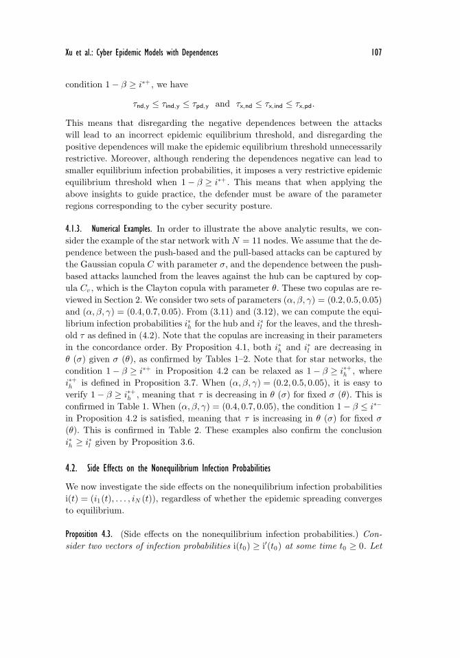
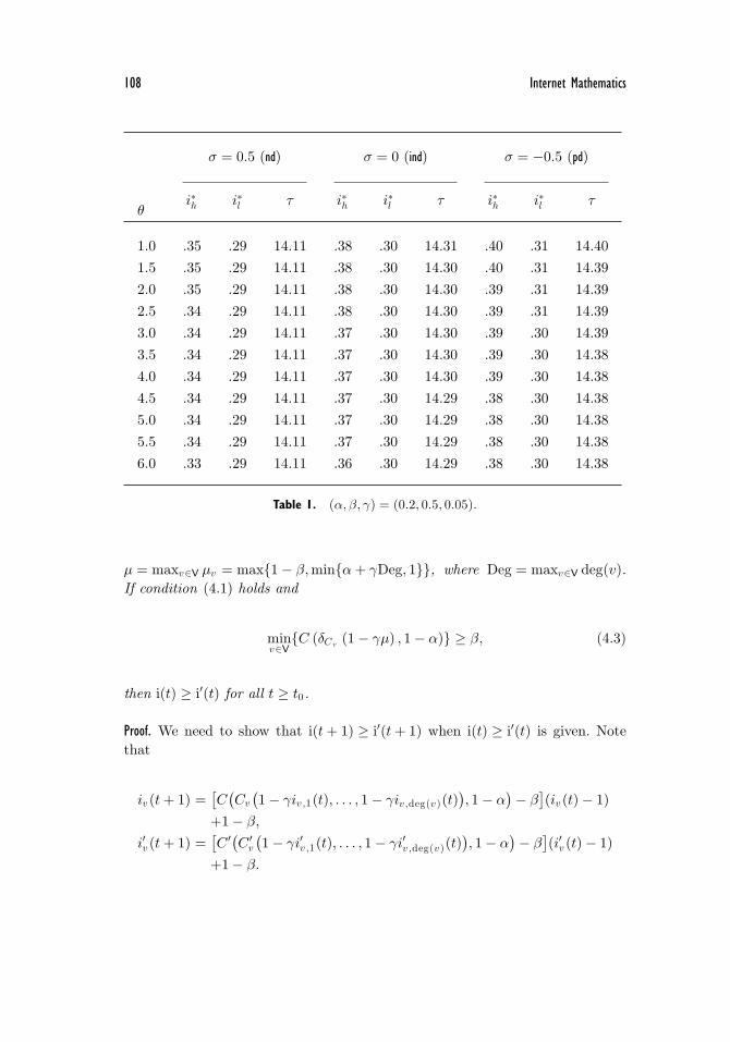
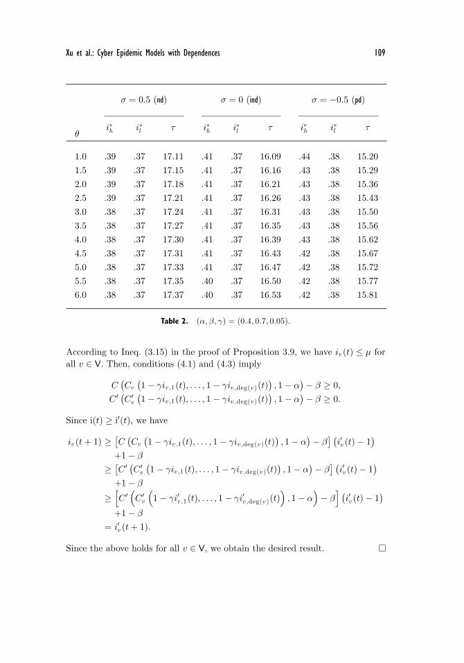
4.1.3. Numerical Examples. In order to illustrate the above analytic results, we con-sider the example of the star network with N = 11 nodes. We assume that the de-pendence between the push-based and the pull-based attacks can be captured bythe Gaussian copula C with parameter σ, and the dependence between the push-based attacks launched from the leaves against the hub can be captured by cop-ula Cv , which is the Clayton copula with parameter θ. These two copulas are re-viewed in Section 2. We consider two sets of parameters (α, β, γ) = (0.2, 0.5, 0.05)and (α, β, γ) = (0.4, 0.7, 0.05). From (3.11) and (3.12), we can compute the equi-librium infection probabilities i∗h for the hub and i∗l for the leaves, and the thresh-old τ as defined in (4.2). Note that the copulas are increasing in their parametersin the concordance order. By Proposition 4.1, both i∗h and i∗l are decreasing inθ (σ) given σ (θ), as confirmed by Tables 1–2. Note that for star networks, thecondition 1 − β ≥ i∗+ in Proposition 4.2 can be relaxed as 1 − β ≥ i∗+h , wherei∗+h is defined in Proposition 3.7. When (α, β, γ) = (0.2, 0.5, 0.05), it is easy toverify 1 − β ≥ i∗+h , meaning that τ is decreasing in θ (σ) for fixed σ (θ). This isconfirmed in Table 1. When (α, β, γ) = (0.4, 0.7, 0.05), the condition 1 − β ≤ i∗−
in Proposition 4.2 is satisfied, meaning that τ is increasing in θ (σ) for fixed σ
(θ). This is confirmed in Table 2. These examples also confirm the conclusioni∗h ≥ i∗l given by Proposition 3.6.
4.2. Side Effects on the Nonequilibrium Infection Probabilities
We now investigate the side effects on the nonequilibrium infection probabilitiesi(t) = (i1(t), . . . , iN (t)), regardless of whether the epidemic spreading convergesto equilibrium.
Proposition 4.3. (Side effects on the nonequilibrium infection probabilities.) Con-sider two vectors of infection probabilities i(t0) ≥ i′(t0) at some time t0 ≥ 0. Let
108 Internet Mathematics
σ = 0.5 (nd) σ = 0 (ind) σ = −0.5 (pd)
θi∗h i∗l τ i∗h i∗l τ i∗h i∗l τ
1.0 .35 .29 14.11 .38 .30 14.31 .40 .31 14.401.5 .35 .29 14.11 .38 .30 14.30 .40 .31 14.392.0 .35 .29 14.11 .38 .30 14.30 .39 .31 14.392.5 .34 .29 14.11 .38 .30 14.30 .39 .31 14.393.0 .34 .29 14.11 .37 .30 14.30 .39 .30 14.393.5 .34 .29 14.11 .37 .30 14.30 .39 .30 14.384.0 .34 .29 14.11 .37 .30 14.30 .39 .30 14.384.5 .34 .29 14.11 .37 .30 14.29 .38 .30 14.385.0 .34 .29 14.11 .37 .30 14.29 .38 .30 14.385.5 .34 .29 14.11 .37 .30 14.29 .38 .30 14.386.0 .33 .29 14.11 .36 .30 14.29 .38 .30 14.38
Table 1. (α, β, γ) = (0.2, 0.5, 0.05).
μ = maxv∈V μv = max{1 − β,min{α+ γDeg, 1}}, where Deg = maxv∈V deg(v).If condition (4.1) holds and
minv∈V
{C (δCv(1 − γμ) , 1 − α)} ≥ β, (4.3)
then i(t) ≥ i′(t) for all t ≥ t0 .
Proof. We need to show that i(t+ 1) ≥ i′(t+ 1) when i(t) ≥ i′(t) is given. Notethat
iv (t+ 1) =[C
(Cv
(1 − γiv,1(t), . . . , 1 − γiv,deg(v )(t)
), 1 − α
) − β](iv (t) − 1)
+1 − β,
i′v (t+ 1) =[C ′(C ′
v
(1 − γi′v ,1(t), . . . , 1 − γi′v ,deg(v )(t)
), 1 − α
) − β](i′v (t) − 1)
+1 − β.
Xu et al.: Cyber Epidemic Models with Dependences 109
σ = 0.5 (nd) σ = 0 (ind) σ = −0.5 (pd)
θi∗h i∗l τ i∗h i∗l τ i∗h i∗l τ
1.0 .39 .37 17.11 .41 .37 16.09 .44 .38 15.201.5 .39 .37 17.15 .41 .37 16.16 .43 .38 15.292.0 .39 .37 17.18 .41 .37 16.21 .43 .38 15.362.5 .39 .37 17.21 .41 .37 16.26 .43 .38 15.433.0 .38 .37 17.24 .41 .37 16.31 .43 .38 15.503.5 .38 .37 17.27 .41 .37 16.35 .43 .38 15.564.0 .38 .37 17.30 .41 .37 16.39 .43 .38 15.624.5 .38 .37 17.31 .41 .37 16.43 .42 .38 15.675.0 .38 .37 17.33 .41 .37 16.47 .42 .38 15.725.5 .38 .37 17.35 .40 .37 16.50 .42 .38 15.776.0 .38 .37 17.37 .40 .37 16.53 .42 .38 15.81
Table 2. (α, β, γ) = (0.4, 0.7, 0.05).
According to Ineq. (3.15) in the proof of Proposition 3.9, we have iv (t) ≤ μ forall v ∈ V. Then, conditions (4.1) and (4.3) imply
C(Cv
(1 − γiv,1(t), . . . , 1 − γiv,deg(v )(t)
), 1 − α
) − β ≥ 0,C ′ (C ′
v
(1 − γiv,1(t), . . . , 1 − γiv,deg(v )(t)
), 1 − α
) − β ≥ 0.
Since i(t) ≥ i′(t), we have
iv (t+ 1) ≥ [C
(Cv
(1 − γiv,1(t), . . . , 1 − γiv,deg(v )(t)
), 1 − α
) − β] (i′v (t) − 1
)+1 − β
≥ [C ′ (C ′
v
(1 − γiv,1(t), . . . , 1 − γiv,deg(v )(t)
), 1 − α
) − β] (i′v (t) − 1
)+1 − β
≥[C ′
(C ′v
(1 − γi′v ,1(t), . . . , 1 − γi′v ,deg(v )(t)
), 1 − α
)− β
] (i′v (t) − 1
)+1 − β
= i′v (t+ 1).
Since the above holds for all v ∈ V, we obtain the desired result.
110 Internet Mathematics
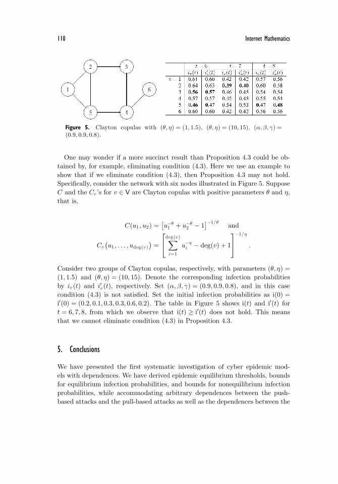
Figure 5. Clayton copulas with (θ, η) = (1, 1.5), (θ, η) = (10, 15), (α, β, γ) =(0.9, 0.9, 0.8).
One may wonder if a more succinct result than Proposition 4.3 could be ob-tained by, for example, eliminating condition (4.3). Here we use an example toshow that if we eliminate condition (4.3), then Proposition 4.3 may not hold.Specifically, consider the network with six nodes illustrated in Figure 5. SupposeC and the Cv ’s for v ∈ V are Clayton copulas with positive parameters θ and η,that is,
C(u1 , u2) =[u−θ1 + u−θ2 − 1
]−1/θ and
Cv(u1 , . . . , udeg(v )
)=
⎡⎣deg(v )∑i=1
u−ηi − deg(v) + 1
⎤⎦−1/η
.
Consider two groups of Clayton copulas, respectively, with parameters (θ, η) =(1, 1.5) and (θ, η) = (10, 15). Denote the corresponding infection probabilitiesby iv (t) and i′v (t), respectively. Set (α, β, γ) = (0.9, 0.9, 0.8), and in this casecondition (4.3) is not satisfied. Set the initial infection probabilities as i(0) =i′(0) = (0.2, 0.1, 0.3, 0.3, 0.6, 0.2). The table in Figure 5 shows i(t) and i′(t) fort = 6, 7, 8, from which we observe that i(t) ≥ i′(t) does not hold. This meansthat we cannot eliminate condition (4.3) in Proposition 4.3.
5. Conclusions
We have presented the first systematic investigation of cyber epidemic mod-els with dependences. We have derived epidemic equilibrium thresholds, boundsfor equilibrium infection probabilities, and bounds for nonequilibrium infectionprobabilities, while accommodating arbitrary dependences between the push-based attacks and the pull-based attacks as well as the dependences between the
Xu et al.: Cyber Epidemic Models with Dependences 111
push-based attacks. In particular, we showed that disregarding the due depen-dences can render the results thereof unnecessarily restrictive or even incorrect.
Our study brings up a range of interesting research problems for further work.First, our characterization study assumes that the dependence or copula struc-tures are given. It is important to know which dependence structures are more rel-evant than the others, in practice. Second, it is ideal to obtain closed-form resultson the equilibrium infection probabilities and the nonequilibrium infection prob-abilities. Third, if we cannot derive closed-form results for the (non)equilibriuminfection probabilities, it is important to seek bounds for these probabilities andsystematically analyze their tightness.
Funding. This work was supported in part by ARO Grants #W911NF-12-1-0286and #W911NF-13-1-0141, and by AFOSR Grant #FA9550-09-1-0165.
References
[1] D. Chakrabarti, Y. Wang, C. Wang, J. Leskovec, and C. Faloutsos. “EpidemicThresholds in Real Networks.” ACM Trans. Inf. Syst. Secur. 10:4 (2008), 1–26.
[2] U. Cherubini, E. Luciano, and W. Vecchiato. Copula Methods in Finance. NewYork, NY: Wiley, 2004.
[3] D. Cvetkovic, P. Rowlingson, and S. Simic. An Introduction to the Theory of GraphSpectra. Cambridge, UK: Cambridge University Press, 2010.
[4] G. Da, M. Xu, and S. Xu. “A New Approach to Modeling and Analyzing Securityof Networked Systems.” In Proc. 2014 Symposium and Bootcamp on the Scienceof Security (HotSoS’14), to appear.
[5] A. Ganesh, L. Massoulie, and D. Towsley. “The Effect of Network Topology onthe Spread of Epidemics.” In Proceedings of IEEE Infocom, 2005. IEEE, 2005.
[6] A. Granas and J. Dugundji. Fixed Point Theory. New York, NY: Springer-Verlag,2003.
[7] H. Joe. “Multivariate Models and Dependence Concepts.” In Monographs onStatistics and Applied Probability, Vol. 73. London, UK: Chapman & Hall, 1997.
[8] J. Kephart and S. White. “Directed-Graph Epidemiological Models of ComputerViruses. IEEE Symposium on Security and Privacy, pp. 343–361. IEEE, 1991.
[9] W. Kermack and A. McKendrick. “A Contribution to the Mathematical Theoryof Epidemics.” Proc. of Roy. Soc. Lond. A 115(1927), 700–721.
[10] X. Li, T. Parker, and S. Xu. “A Stochastic Model for Quantitative Security Anal-ysis of Networked Systems.” In IEEE Transactions on Dependable and SecureComputing, 8:1(2011), 28–43.
[11] C. R. MacCluer. “The Many Proofs and Applications of Perron’s Theorem.” SIAMReview 42 (2000), 487–498.
112 Internet Mathematics
[12] A. McKendrick. “Applications of Mathematics to Medical Problems.” Proc. ofEdin. Math. Society 14(1926), 98–130.
[13] A. J. McNeila and J. Neslehova. “Multivariate Archimedean Copulas, d-MonotoneFunctions and l1-Norm Symmetric Distributions.” Annals of Statistics 37(2009),3059–3097.
[14] R. B. Nelsen. An Introduction to Copulas, Second Edition. Springer Series inStatistics. New York, NY: Springer, 2006.
[15] P. Van Mieghem, J. Omic, and R. Kooij. “Virus Spread in Networks.” IEEE/ACMTransactions on Networking 17:1(2009), 1–14.
[16] Y. Wang, D. Chakrabarti, C. Wang, and C. Faloutsos. “Epidemic Spreading inReal Networks: An Eigenvalue Viewpoint.” In Proc. of the 22nd IEEE Symposiumon Reliable Distributed Systems (SRDS’03), pp. 25–34. IEEE, 2003.
[17] M. Xu and S. Xu. “An Extended Stochastic Model for Quantitative Security Anal-ysis of Networked Systems.” Internet Mathematics 8:3(2012), 288–320.
[18] S. Xu, W. Lu, and L. Xu. “Push- and Pull-based Epidemic Spreading in Net-works: Thresholds and Deeper Insights.” ACM Transactions on Autonomous andAdaptive Systems (ACM TAAS) 7:3(2012), 32.
[19] S. Xu, W. Lu, and Z. Zhan. “A Stochastic Model of Multivirus Dynamics.” IEEETrans. Dependable Sec. Comput. 9:1(2012), 30–45.
Maochao Xu, Department of Mathematics, Illinois State University, 100 North Univer-sity Street, Normal, IL 61790, USA ([email protected])
Gaofeng Da, Institute for Cyber Security, University of Texas at San Antonio, OneUTSA Circle, San Antonio, TX 78249, USA ([email protected])
Shouhuai Xu, Department of Computer Science, University of Texas at San Antonio,One UTSA Circle, San Antonio, TX 78249, USA ([email protected])