Curves and surfaces & modeling case studies

Karan Singh

2

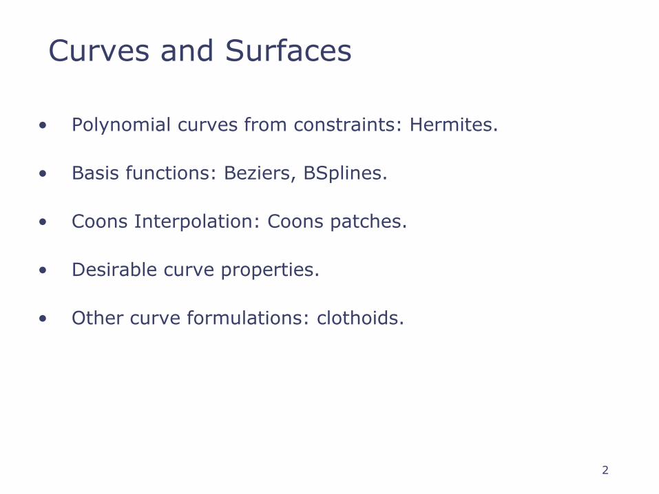
Curves and Surfaces

• Polynomial curves from constraints: Hermites.

• Basis functions: Beziers, BSplines.

• Coons Interpolation: Coons patches.

• Desirable curve properties.

• Other curve formulations: clothoids.

3

Parametric Polynomial Curves

Recall a linear curve (line) is: p(t) = a1t+a0

A cubic curve is similarly:

…or p(t) = d3t3+d2t

2 +d1t+d0 , where di = [ai, bi, ci,]T

Cubics are commonly used in graphics because:

• curves of lower order have too little flexibility (only planar, no curvature control).

• curves of higher order are unnecessarily complex and easily wiggle.

Polynomial curves from constraints

p(t) = TA , where T is powers of t. for a cubic T=[t3 t2 t1 1].

Written with geometric constraints p(t) = TMG, where M is the Basis matrix of the curve, G the design constraints.

An example of constraints for a cubic Hermite for eg. areend points and end tangents. i.e. P1,R1 at t=0 and P4,R4 at t=1.Plugging these constraints into p(t) = TA we get.

Hp(0) = P1 = [ 0 0 0 1 ] A p(1) = P4 = [ 1 1 1 1 ] A TA=TMG &p'(0)= R1 = [ 0 0 1 0 ] A => G=HA => H=M-1

p'(1)= R4 = [ 3 2 1 0 ] A

Bezier Basis Matrix

A cubic Bezier can be defined with four points where:P1,R1 at t=0 and P4,R4 at t=1 for a Hermite.R1 = 3(P2-P1) and R4 = 3(P4-P3).

We can thus compute the Bezier Basis Matrix by finding the matrix that transforms [P1 P2 P3 P4 ]T into [P1 P4 R1 R4 ] T i.e.

B_H = [ 1 0 0 0 ][ 0 0 0 1][-3 3 0 0][ 0 0 -3 3]

Mbezier=Mhermite * B_H

Bezier Basis Functions

[ -1 3 -3 1 ][ 3 -6 3 0 ] [ -3 3 0 0 ] [ 1 0 0 0 ]

The columns of the Basis Matrix form Basis Functions such that:p(t)= B1(t)P1 + B2(t)P2 + B3(t)P3 + B4(t)P4.

From the matrix:

Bi+1(t) = (n) *(1-t)(n-i)

*ti

i

…also called Bernstein polynomials.

B1

B2

B2

B3

Basis Functions

Basis functions can be thought of as an influence weight that eachconstraint has as t varies.

Note: actual interpolation of any constraint only happens if its Basisfunction is 1 and all others are zero at some t.

Often Basis functions for design curves sum to 1 for all t.This gives the curve some nice properties like affine invarianceand the convex hull property when the functions are additionallynon-negative.

Bezier Patches

Using same data array P=[pij] as with interpolating form:

Patch lies in

convex hull

p(u,v) = Si Sj Bi(u) Bj(v) pij = uT B P BT v

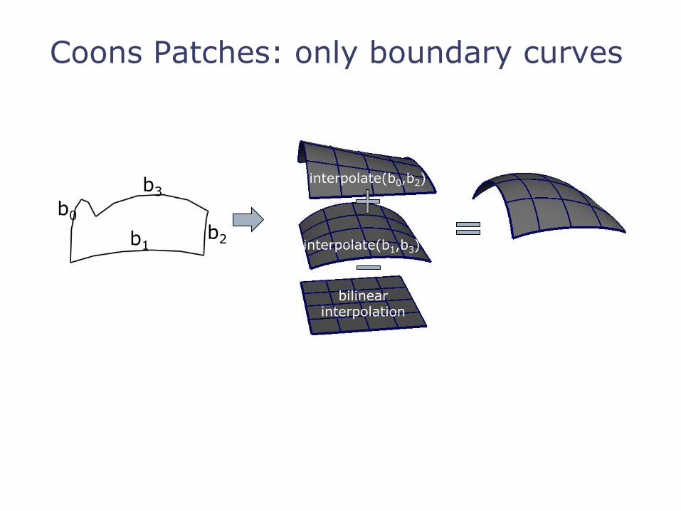
Coons Patches: only boundary curves

b0

b3

b2b1

interpolate(b0,b2)

interpolate(b1,b3)

bilinearinterpolation

Traditional Splines

BSpline Basis Functions

• Can be chained together.• Local control (windowing).

Bezier vs. BSpline

Bezier

BSpline

Representing a conic as a polynomial

• <x(t),y(t)> = < cos(t), sin(t) >

• Taylor series for sin(t)= t -t3/3! + t5/5! …

• u=tan(t/2)

• <x(u),y(u)> = < (1-u2)/(1+u2) , 2u/(1+u2) >

• Rational Bspline’s are defined with homogeneous coordinates using w(t).

• NURBS additionally adds non-uniform knots.

Curve Design Issues

• Continuity (smoothness, fairness and neatness).

• Control (local vs. global).

• Interpolation vs. approximation of constraints.

• Other geometric properties (planarity, invariance).

• Efficient analytic representation.

15

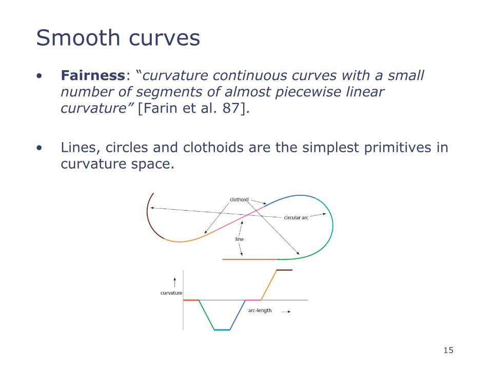
Smooth curves

• Fairness: “curvature continuous curves with a small number of segments of almost piecewise linear curvature” [Farin et al. 87].

• Lines, circles and clothoids are the simplest primitives in curvature space.

16

Clothoids

Sketch curves often represent gestural information or capture design intent where the overall stroke appearance (fairness) is more important than the precise input.

[McCrae & Singh, Sketching Piecewise Clothoid Curves, SBIM 2008]http://www.dgp.toronto.edu/~mccrae/clothoid/

17

What are Clothoids?

• Curves whose curvature changes linearly with arc-length.

• Described by Euler in 1774, a.k.a. Euler spiral.

• Studied in diffraction physics, transportation engineering (constant lateral acceleration) and robot vehicle design (linear steering).

18

Comparative approaches to fairing

19

Approach

20

Approach

Segment

21

Approach

Segment Assemble

22

Approach

Segment

Align

Assemble

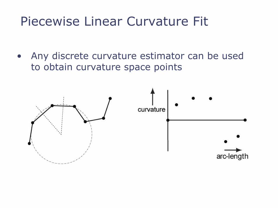
Piecewise Linear Curvature Fit

• Any discrete curvature estimator can be used to obtain curvature space points

Piecewise Linear Curvature Fit

• Find a small number of connected line segments that minimize fit error.

Piecewise Linear Curvature Fit

• Dynamic programming (cost of fit matrix M):

Efit(a,b) is the fitting error of a line to points a..b.

Ecost is the penalty incurred to increment the number of line segments.

Can be used to fit other primitives like circle involute.

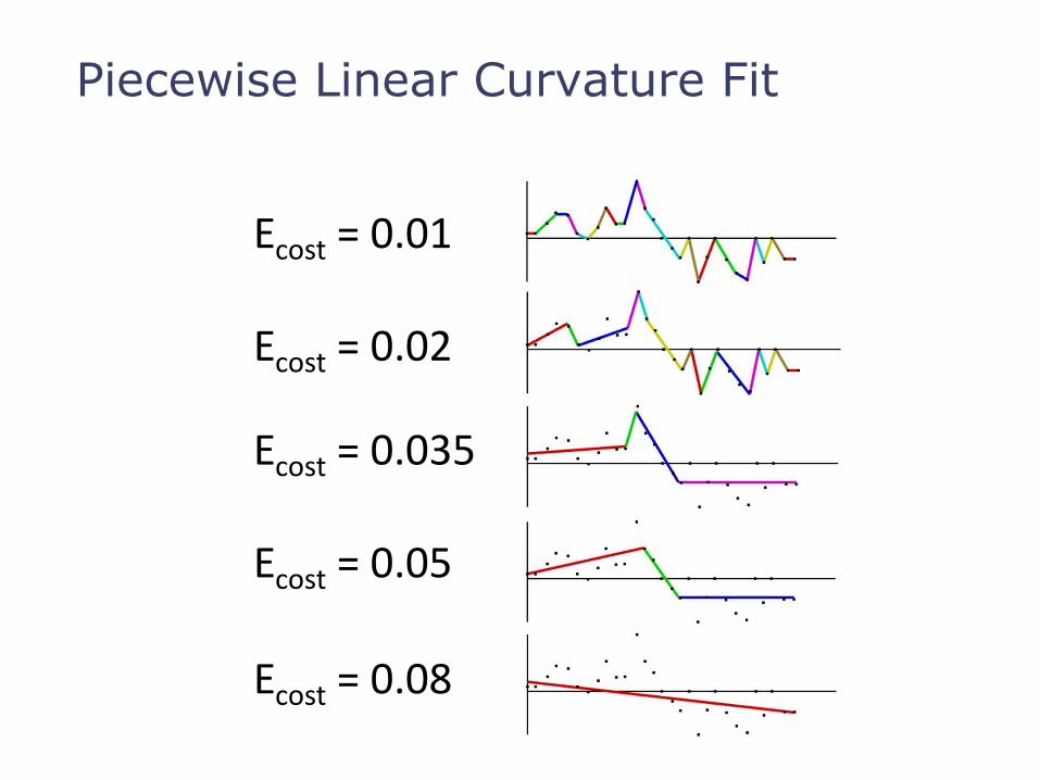
Piecewise Linear Curvature Fit

Ecost = 0.01

Ecost = 0.02

Ecost = 0.035

Ecost = 0.05

Ecost = 0.08

Assembly

• To assemble piecewise clothoid curve:

• Map each curvature space line segment to a unique line, circle or clothoid curve segment.

• Attach segments so they are position/tangent continuous

• Resulting curve has G2 continuity

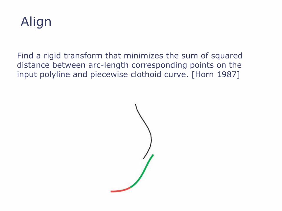
Align

Find a rigid transform that minimizes the sum of squared distance between arc-length corresponding points on the input polyline and piecewise clothoid curve. [Horn 1987]

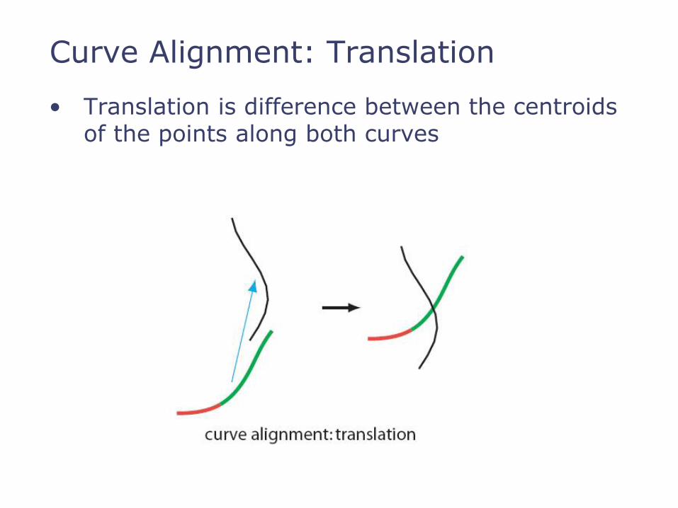
Curve Alignment: Translation

• Translation is difference between the centroids of the points along both curves

Curve Alignment: Rotation

• Rotation minimizes weighted squared distances:

• Optimal A given by:

• Rotation R extracted as,where

31

Model creation categories

• Suggestive systems

• Input compared to template objects

• symbolic or visual memory

• Constructive systems

• Input directly used to create object

• perceptual or visual rules

32

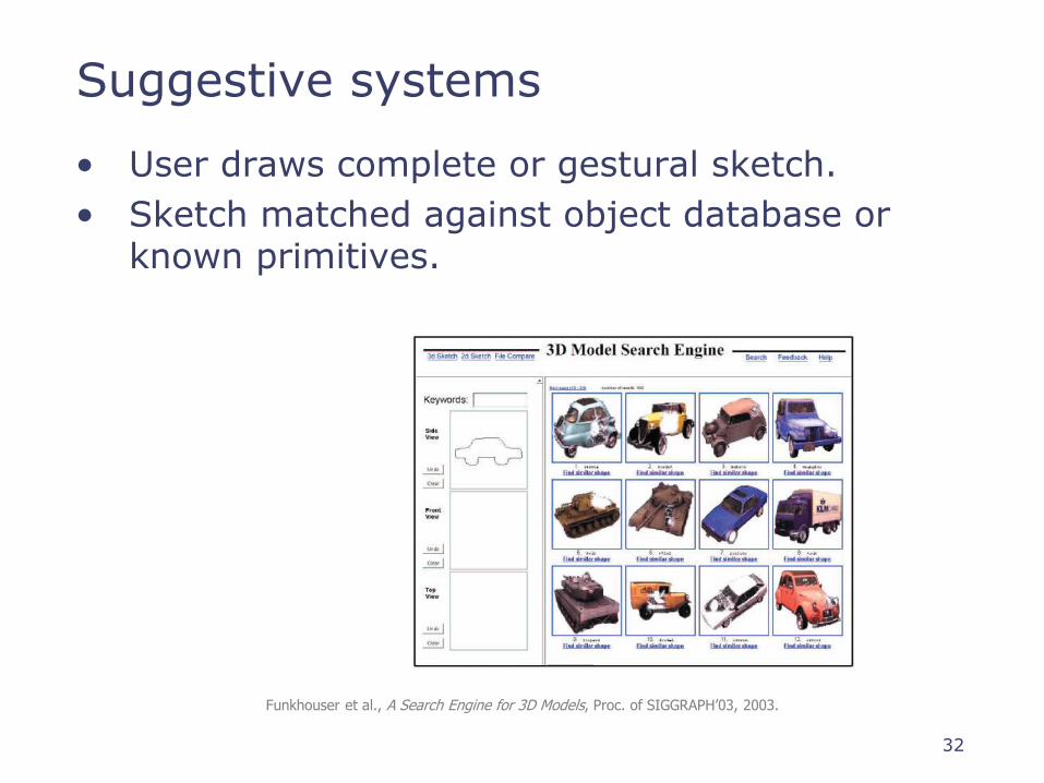
Suggestive systems

• User draws complete or gestural sketch.

• Sketch matched against object database or known primitives.

Funkhouser et al., A Search Engine for 3D Models, Proc. of SIGGRAPH’03, 2003.

33

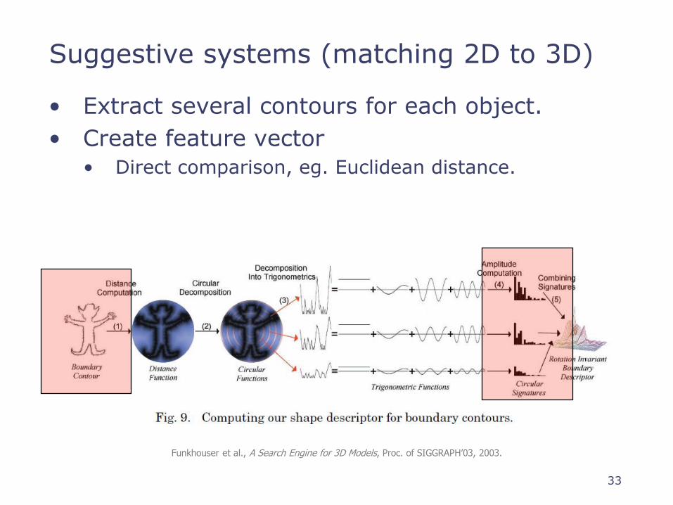
Suggestive systems (matching 2D to 3D)

• Extract several contours for each object.

• Create feature vector

• Direct comparison, eg. Euclidean distance.

Funkhouser et al., A Search Engine for 3D Models, Proc. of SIGGRAPH’03, 2003.

34

Constructive systems

• Rules and constraints rather than templates:

• Restricting application domain (eg. sketching roads).

• Restricting object type (eg. mechanical or organic).

• Restricting task (eg. smoothing, cutting or joining).

M. Masry and H. Lipson, A Sketch-Based Interface for Iterative Design and Analysis of 3D Objects, EG SBIM’05, 2005.

T. Igarashi et al., Teddy: A Sketching Interface for 3D Freeform Design, Proc. of SIGGRAPH’99, 1999.

35

Case Studies

• Drive.

• Teddy, Fibermesh.

• ILoveSketch.

• Analytic drawing.

• True2Form.

• SecondSkin.

Drive: single-view sketching

A sketch-based system to create conceptual layouts of 3D path networks.

Drive features

Elegant interface:

open stroke = path

closed stroke = selection-action menu.

Piecewise clothoid path construction.

Crossing paths.

Break-out lens. (single-view context)

Terrain sensitive sketching.

[McCrae & Singh, Sketching based Path Design, Graphics Interface 2009]

Drive

[McCrae & Singh, Sketching based Path Design, Graphics Interface 2009]

39

Teddy

• Teddy inflates a closed 2D stroke like blowing up a balloon.

T. Igarashi et al., Teddy: A Sketching Interface for 3D Freeform Design, Proc. of SIGGRAPH’99, 1999.

40

Inflation

• Offset surface proportionally to distance from spine of the contour

• Produces smooth blobby objects

Igarashi et al., Teddy: A Sketching Interface for 3D Freeform Design, SIGGRAPH’99, 1999.

41

Skeleton extraction

• Delaunay triangulation

• Chordal axis transform

Igarashi et al., Teddy: A Sketching Interface for 3D Freeform Design, SIGGRAPH’99, 1999.

Polygon approximation

Delaunay

Skeleton

42

Trouble with contours and silhouettes

• Rarely planar.

• Can contain T-junctions and cusps.

• Occlusion.

43

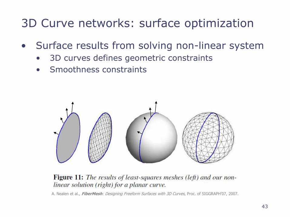
3D Curve networks: surface optimization

• Surface results from solving non-linear system

• 3D curves defines geometric constraints

• Smoothness constraints

A. Nealen et al., FiberMesh: Designing Freeform Surfaces with 3D Curves, Proc. of SIGGRAPH’07, 2007.

44

FiberMesh

• User can specify additional curves on the surface

• Further constraints that define the surface

• Sharp features

A. Nealen et al., FiberMesh: Designing Freeform Surfaces with 3D Curves, Proc. of SIGGRAPH’07, 2007.

45

ISKETCH: multi-view sketching

46

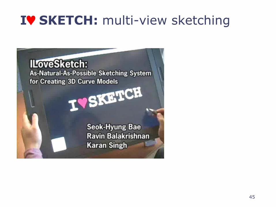
ISKETCH: multi-view sketching

A judicious leap from 2D to 3D.

• Presents a virtual 2D sketchbook with simple paper navigation and automatic rotation for ergonomic pentimenti style 2D sketching.

• Seamless transition to 3D with a suite of multi-view curve sketching tools with context switching based on sketchability.

[Bae, Balakrishnan & Singh, ILoveSketch: As-natural-as-possible

sketching system for creating 3D curve models. UIST 2008]www.ilovesketch.com

47

ISKETCH : epi-polar symmetry

48

ISKETCH (at SIGGRAPH 09 eTech)

100 models created over 4 days (made public for research)http://www.dgp.toronto.edu/~shbae/ilovesketch_siggraph2009.htm

49

Experts and drawing systems

50

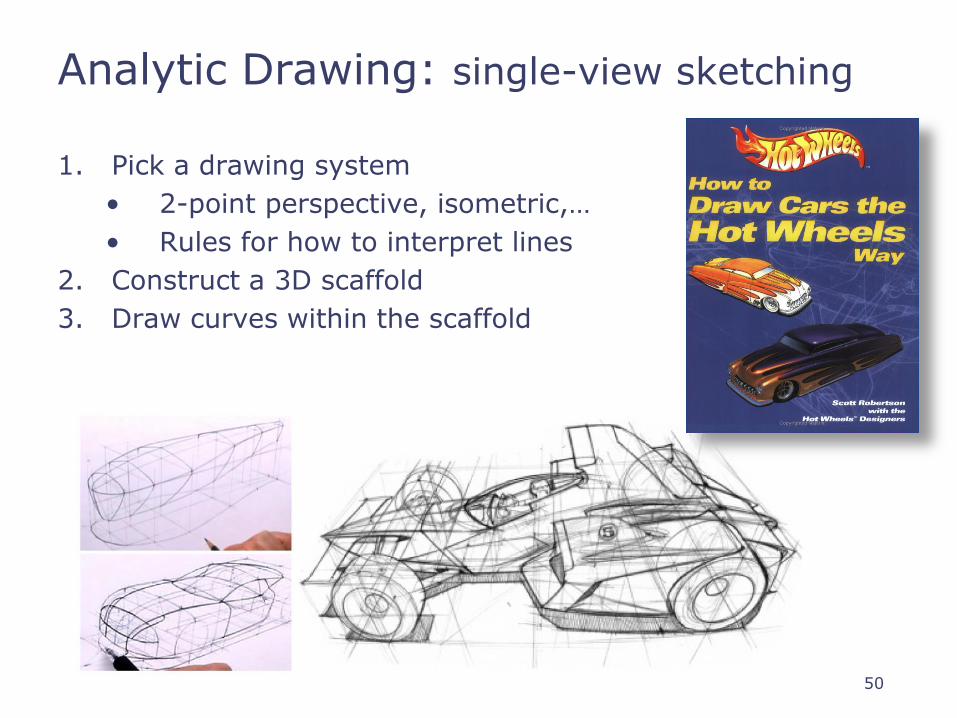
Analytic Drawing: single-view sketching

1. Pick a drawing system

• 2-point perspective, isometric,…

• Rules for how to interpret lines

2. Construct a 3D scaffold

3. Draw curves within the scaffold

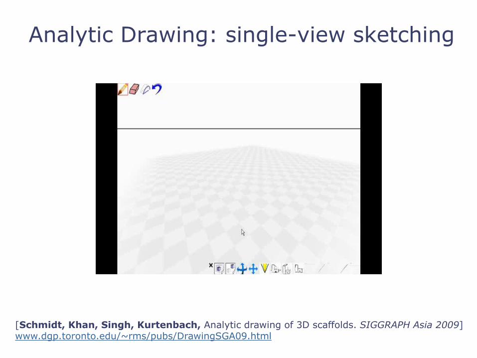
Analytic Drawing: single-view sketching

[Schmidt, Khan, Singh, Kurtenbach, Analytic drawing of 3D scaffolds. SIGGRAPH Asia 2009]www.dgp.toronto.edu/~rms/pubs/DrawingSGA09.html

Analytic Drawing: single-view sketching

[Schmidt, Khan, Singh, Kurtenbach, Analytic drawing of 3D scaffolds. SIGGRAPH Asia 2009]www.dgp.toronto.edu/~rms/pubs/DrawingSGA09.html

Scaffold constraints: position, direction, length.

Geometric priors: lines, circular-arcs.

Probabilistic model: redundancy resolves ambiguity.

Analytic Drawing: inference

concept sketch• Explore form.• Fast to draw.

presentation rendering• Communicate with clients.• Tedious, repetitive, painting.

CrossShade/True2Form: design sketches©www.sketch-a-day.com

CrossShade: 3D presentation rendering

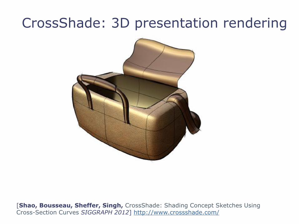
CrossShade: 3D presentation rendering

[Shao, Bousseau, Sheffer, Singh, CrossShade: Shading Concept Sketches Using Cross-Section Curves SIGGRAPH 2012] http://www.crossshade.com/

CrossShade: design analysis

“Cross-sections on a surface explain or emphasize its curvature.”

“…bend or transform the object’s surface.”

CrossShade: perceptual study

Viewers are persistent, consistent and accurate in X-hair perception.

CrossShade: defining cross-hairs

Plane Orthogonality Local curvature lines

Local Geodesics Minimal Foreshortening

Orientation

CrossShade: Algorithm

CrossShade: Algorithm

• Compute X-section planes, X-hair normals: use 5 properties.

CrossShade: Algorithm

• Compute X-section planes, X-hair normals: use 5 properties.

• Propagate normals along X-section curves: minimize twist.

CrossShade: Algorithm

• Compute X-section planes, X-hair normals: use 5 properties.

• Propagate normals along X-section curves: minimize twist.

• Propagate normals into interior regions: Coons interpolation.

CrossShade: Algorithm

• Compute X-section planes, X-hair normals: use 5 properties.

• Propagate normals along X-section curves: minimize twist.

• Propagate normals into interior regions: Coons interpolation.

• Shade!

CrossShade: Results

[Xu, Chang, Bousseau, McCrae, Sheffer, Singh, True2Form: 3D curve networks from 2D sketches via selective regularization. SIGGRAPH 2014]

True2Form: 3D rendering modeling

2D sketch Crossshade True2Form True2Formside view 3D side view 3D input overlay

T2F: descriptive curve properties => 3D

Fidelity: sketches reflect 3D geometry.

• Satisfied by flat interpretation.

Regularity: curves often capture 3D constraints.

• This lifts curves to 3D.

• Regularity is context-based.

True2Form: perceptual validation

Viewers consistently perceive 3D parallelism, symmetry,orthogonality, linearity and planarity cues in 2D sketches.

True2Form: fidelity and regularity

Curve network surfacing

Determine cyclesPatch cycles

[Bessmeltsev, Wang, Sheffer, Singh, Design-Driven Quadrangulation of Closed 3D Curves.SIGGRAPH Asia 2012]

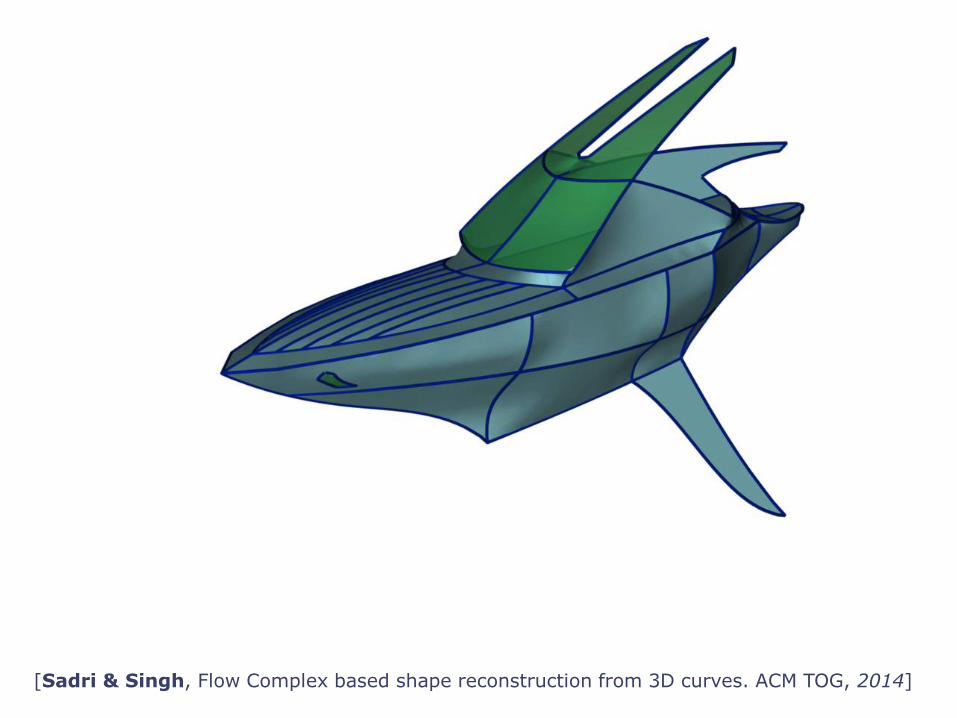
[Sadri & Singh, Flow Complex based shape reconstruction from 3D curves. ACM TOG, 2014]

SecondSkin: layered 3D modeling

[DePaoli & Singh, SecondSkin: Sketch-based Construction of Layered 3D Models. SIGGRAPH, 2015]

SecondSkin: layered 3D modeling

Sketch-based modeling ingredients

System Fidelity Geom. priors Perceived Regularity

View

Teddy/FM Planarity Fixed depth Project onmesh

Multi-view

ILoveSketch Cubic Bezier Symmetry Multi-view

Analytic 3D Proj. accuracy Length,direction,circular arcs

Scaffold Single-view

True2Form Proj. accuracy,Min. variation

OrthogonalX-hairs etc.

Single-view

SecondSkin Foreshortening Cubic Bezier Underlying geom. & curves

Multi-view

Key Messages

• Centuries of visual experience captured in artistic practice.

• Perceived regularity.

• Techniques based on artistic and perceptual insights, andleaving user ultimate creative control.

• Better tools = Better VIDEO OUT Better tools != Better content