Current Account Assessments: Methodologies and Issues

Luis Catão IMF Research Department

June 2012

The views expressed here do not necessarily reflect those of the IMF, its board of directors, or management. Much of the material in this presentation draws on work by the open economy division of the research department of the IMF. Thanks to Olivier Blanchard, Jonathan Ostry, Steve Phillips, Luca Ricci, Mitali Das, Jungjin Lee, and IMF seminar attendants for many valuable comments. All errors are mine.

I. Aim of the Presentation

• To provide a encompassing framework that nests existing current account empirical models.

• Distinguish them, with special focus on extensions

underpinning the external balance assessment (EBA) methodology recently developed by IMF staff.

• Evaluation of these extensions, esp. the interpretation of regression residuals and the role of policy “gaps”.

• Discuss further extensions.

Presentation’s Road Map

I. The S-I Framework:

Bare-Bone Models (IMF’s CGER) & Extensions (inc. EBA pilot model) II. Data and Estimation Approach

III. Gap Estimates and Robustness IV. Interpreting Residuals

V. Road Ahead

II. The S-I Model

• Long-standing work-horse, in the IMF and elsewhere (Isard and Faruquee, 1998; Isard et al.; 2001; Chinn & Prasad, 2003; Bussière et al., 2004; Lee et al., 2008; Christiansen et al, 2009; Brissimis et al., 2010; Cheung et al., 2010)

• Used in its bare-bone form in the IMF CGER assessments; variants in recent work on imbalances (Chinn et al, 2011; Lane and Milesi-Ferretti, 2012)

• EBA: extends CGER to take into account global capital market cycles and the role of policy in current account (CA) “gaps”.

• All these models can be nested in 1 behavioral equation, 3 accounting constraints, and 1 policy rule equation:

I-S: (1) BOP constraint: (2) Solvency constraint: (3) Multilateral Constraint: (4)

( , ) ( , , ) ( , , )wos I

CA S Ireer y nfa r x r reer xY Y Y

= −

( , ) ( , ) Rewo woCF

CA FAreer y r r x sY Y

+ − = ∆

*11 (1 )t j t j

t t t k t jkj t j t j

s anfa E tb

rρ

ρ

∞ ∞+ +

+ +== + +

= − ∏ + +

∑

1 1

0N N

ii i

i i i

CACAY

ω= =

= =∑ ∑

where Policy rule: If IT: (5a) If peg: (5b) --> So, the output gap enters via the policy rule.

1

1 , iN

ij

jω

=

= ∀∑

( )Nt y t tr r yα λ ς= + + +

1 1 1( ) ( )

( , )

wo wo wot t t t t t

wo wot t t

r i E r Er f y y

π π π+ + += − = − −

= −

Without the multilateral constraint, the model solves for

4 variables: CA, REER, NFA, and r. The reduced-form CA equation is: (6)

( , , , , , , , )t t t

wo wot t t t t I S CF tca f nfa y y r res= ∆x x x

• The model closes with the zero global CA constraint which is applied by setting the weights in equation (4) to .

• It can be shown that this constraint is met once all variables that don’t up to zero globally (like NFA and TOT) are measured relative to their respective (US$) weighed global average.

• Then variables like the world output gap and real world interest rate drop out from (6).

ii

i

YY

ω =∑

Two important things to note: • One is that the global average counterpart includes

the own country. So, variables are NOT measured relative to ROW.

E.g. if country A accounts for 20% of world GDP, the effects of

its fiscal balance on the current account will be dampened accordingly: γ[X-(0.2X_wo+0.8X_ROW)]

• Still, what typically ROW does matters. So, your

policies may be at desirable levels and you may still have a CA gap due to “mis-behavior” elsewhere.

• This general set-up allows us to see the critical difference between models.

• One is the choice of

• In CGER (as well as Chinn and Prasad, 2003; Chinn et al. 2011; Lane and Milesi-Ferretti, 2012) capital account shifters ( ) had no role.

• The policy “gaps” that enter as I or S shifters (such as capital controls, too little or too much social protection) were not explicitly controlled for.

• They would all go into the residual.

, ,tI s CFx x x

tCFx

Table 1

CGER EBA

Saving shifters (Xs)per capita income X Xdemographics X Xoil balance X Xactual or expected growth X Xfinancial deepeningsocial protection Xfiscal policy X XCommodity TOT gap X

Investment Shifters (Xi)per capita income X Xactual or expected growth X Xgovernance XPublic Investment Share

Capital Account Shifters (XCF)Global Risk Aversion (VIX) XShare in world reserves XCapital Controls X

Output Gap X

Total No of variables 5 12

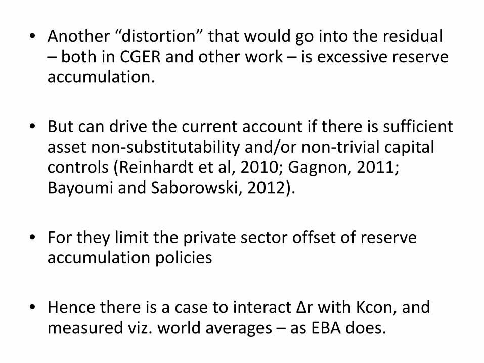
• Another “distortion” that would go into the residual – both in CGER and other work – is excessive reserve accumulation.

• But can drive the current account if there is sufficient asset non-substitutability and/or non-trivial capital controls (Reinhardt et al, 2010; Gagnon, 2011; Bayoumi and Saborowski, 2012).

• For they limit the private sector offset of reserve accumulation policies

• Hence there is a case to interact Δr with Kcon, and measured viz. world averages – as EBA does.

• Another key distinction pertains to the role of actual policies vs. sustainable/desirable policies in (6).

• In CGER (as well as several other studies), the only policy variable (fiscal) was entered as actual rather the sustainable policy (P*).

• But relevant policies are more than just fiscal policy.

• And besides including a host of actual policies variables in

the regression, these need not be their desirable/sustainable levels. Hence some adjustment must be made for that.

• This is what EBA does.

• In EBA, the inclusion of actual NFA in the regression also allows for the inter-temporal budget constraint to play a role.

• From eq. 3.a, this term is positive if r>a, but should be unambiguously negative in the tb equation.

• We show that this holds true in the estimates below.

• But including actual policies in the regression raises the question of how to interpret the regression residual and issue of positive vs normative interpretation thereof. This is discussed below.

II. Data and Estimation

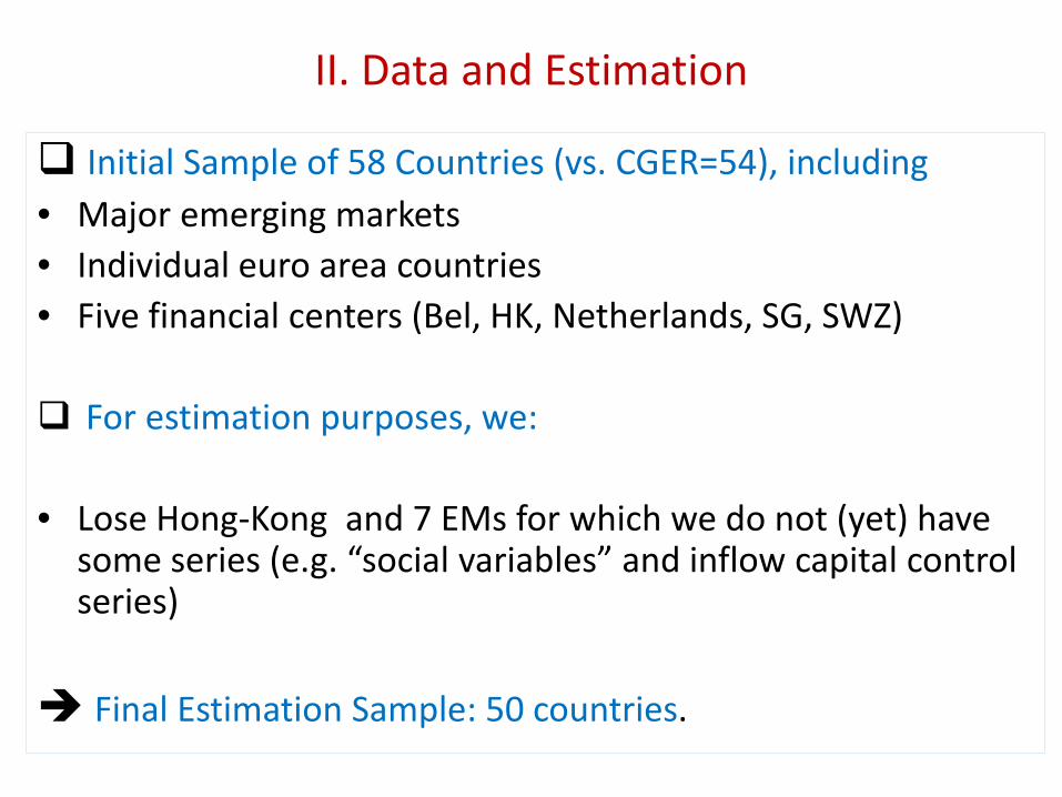
Initial Sample of 58 Countries (vs. CGER=54), including • Major emerging markets • Individual euro area countries • Five financial centers (Bel, HK, Netherlands, SG, SWZ) For estimation purposes, we:

• Lose Hong-Kong and 7 EMs for which we do not (yet) have

some series (e.g. “social variables” and inflow capital control series)

Final Estimation Sample: 50 countries.

Estimation Period: 1986-2010, annual data (CGER as well as Chinn et al., use of 4-year averages) Panel Regressions with no fixed effects and

homogenous slope coefficients (we check that). GLS Estimates with country-specific AR1 correction

and heteroskedastic residuals that are cross-country correlated.

Relevant variables measured viz foreign counterparts to facilitate global consistency, as discussed.

L. NFA/GDP 0.04 ***

L. (NFA/GDP)*(dum=1 if NFA/GDP < -60%) -0.03 **

Financial Center Dummy 0.03 ***

L. Own per capita GDP/US per capita GDP (PPP) 0.04 ***

Oil Trade Balance/GDP (if >10%) 0.48 ***

Dependency Ratio 0.00

Population Growth 0.04

Aging Speed 0.13 ***

Real GDP growth, 5-year ahead forecast -0.40 ***

L.Public Health Spending/GDP -0.57 ***

L.VOX*(1-Kcontrol) 0.06 ***

L.VOX*(1-Kcontrol)*(currency’s share in world reserves stock) -0.16 ***

Own currency’s share in world reserve stock -0.004

Output Gap -0.39 ***

Terms of Trade gap*Trade Openness 0.25 ***

Cyclically Adjusted Fiscal Balance, instrumented 0.42 ***

Capital Control Index ("Kcontrol") 0.03 ***

Kcontrol*(Changes in Reserves)/GDP, instrumented 0.48 **

Constant 0.009

Observations 1099

R-Squared 0.56

RMSE 3.4%

AR(1) 0.68

Number of countries 50

1/ GLS estimates with panel heteroskedasticity corrected standard errors. "L" stands for one-year lag of the respective variable.* significant at 10%; ** significant at 5%; *** significant at 1%

Table 2. EBA Model: Current Account Regression Results 1/

(Estimation Period: 1986-2010)

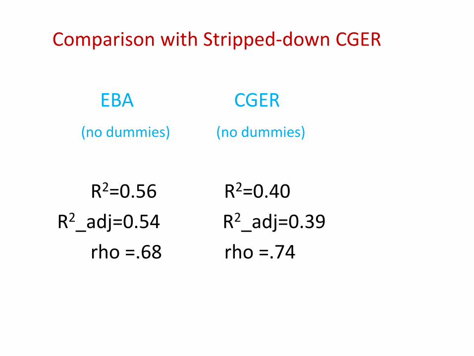
Comparison with Stripped-down CGER EBA CGER (no dummies) (no dummies)

R2=0.56 R2=0.40 R2_adj=0.54 R2_adj=0.39 rho =.68 rho =.74

ARG

AUS

AUT

BELBRA CAN

CHL

CHN

COL

CRI

CZE

DNK

EGY

FIN

FRA

DEU

GTMHUNIND

IDN

IRL

ISR

ITA

JPNKOR

MYS

MEX

MAR

NLD

NZL

NOR

PAK

PER

PHL

POL

PRT

RUS

ZAF

ESP

LKA

SWE

CHE

THA

TUNTUR

GBR

USAURY

-12%

-8%

-4%

0%

4%

8%

12%

16%

-8% -4% 0% 4% 8% 12%

Actu

al C

A/G

DP

Fitted CA/GDP

Figure 1. Actual VS Fitted CA/GDP for 2008-2010

Linear (45 degree +/- 2* RMSE)

Linear ("45 degree - 2 * RMSE")

1 st.dev dev band

-12%

-8%

-4%

0%

4%

8%

12%

16%

-8% -4% 0% 4% 8% 12%

Actu

al C

A/G

DP

Fitted CA/GDP

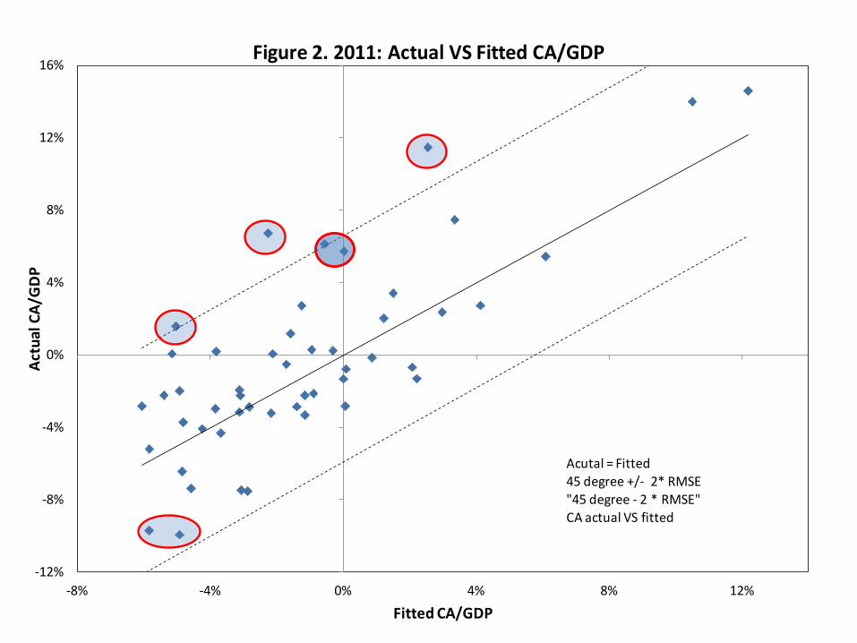
Figure 2. 2011: Actual VS Fitted CA/GDP

Acutal = Fitted45 degree +/- 2* RMSE"45 degree - 2 * RMSE"CA actual VS fitted

Robustness

• Endogeneity/Instrumenting • Homogeneity Assumptions

• Feedback of lagged NFA on TB • Multilateral Consistency

• Two ways of relaxing the (potential) straightjacket of coefficient homogeneity across countries.

1) through variable interaction. E.g.: VIX*Kcon and VIX*Reserve currency, TOT*openness, etc.

Good results there.

2) Relax the assumption that the AR1 coefficient is the same.

Gains seem meagre enough.

Table 3.a Group Specific AR(1) Estimates

Advanced Countries 0.69

Euroarea 0.74

Non-euro Advanced 0.68

Emerging Markets 0.62

Overall Mean 0.66

L. NFA/GDP 0.01

L. (NFA/GDP)*(dum=1 if NFA/GDP < -60%) -0.04 **

Financial Center Dummy 0.03 ***

L. Own per capita GDP/US per capita GDP (PPP) 0.08 ***

Oil Trade Balance/GDP (if >10%) 0.37 ***

Dependency Ratio -0.14 **

Population Growth 0.05

Aging Speed 0.13 ***

Real GDP growth, 5-year ahead forecast -0.30 ***

L.Public Health Spending/GDP -0.11

L.VOX*(1-Kcontrol) 0.06 ***

L.VOX*(1-Kcontrol)*(currency’s share in world reserves stock) -0.18 ***

Own currency’s share in world reserve stock -0.01

Output Gap -0.39 ***

Terms of Trade gap*Trade Openness 0.28 ***

Cyclically Adjusted Fiscal Balance, instrumented 0.80 ***

Capital Control Index ("Kcontrol") 0.03 ***

Kcontrol*(Changes in Reserves)/GDP, instrumented 0.32 *

Constant 0.009

Observations 1099

R-Squared 0.43

RMSE 3.8%

AR(1) 0.78

Number of countries 50

1/ GLS estimates with panel heteroskedasticity corrected standard errors. "L" stands for one-year lag of the respective variable.* significant at 10%; ** significant at 5%; *** significant at 1%

Table 2. EBA Model: Trade Balance Regression Results 1/

(Estimation Period: 1986-2010)

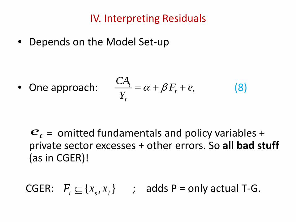
IV. Interpreting Residuals

• Depends on the Model Set-up

• One approach: (8) = omitted fundamentals and policy variables +

private sector excesses + other errors. So all bad stuff (as in CGER)!

CGER: ; adds P = only actual T-G.

tt t

t

CA F eY

α β= + +

te

{ , }t s IF x x⊆

• EBA approach:

EBA gap • So, you proceed in three steps: 1) Estimate (10) to get u, where & P encompasses more than just T-G. 2) Get P* (e.g. from IMF country teams). 3) Then add (P-P*) to in order to obtain the EBA

gap.

* *

(10)

( )

tt t t

t

t t t t t

CA F P uY

F P u P P

α β γ

α β γ γ

= + + +

= + + + + −

γ̂

{ , , , }s I CFnfa⊆F x x x

Four Important Points about EBA gaps

• If u=0 you don’t necessarily give a country a pass if P-P*# 0.

• Pt* has a non-trivial normative content, i.e., means what a country’s desired policy should be, in terms of mitigating/avoid distortions and be “sustainable”.

• Because P* is also measured relative to the world, what others do in terms of their own P* will affect your CA.

• Because of the above and also because u contains our measure of ignorance and possible specification and/or measurement errors, a tolerance band must be allowed, including room for discussion/policy judgment as to the final assessment.

In short: • The policy-adjusted EBA residual now becomes the

relevant assessment metric, rather than .

• As it turns out, often the residual of the reg (10) is typically the dominant component in the EBA gap when that gap is large.

• This again raises the stakes regarding the normative/positive issues in interpreting the residual.

tu

-8%

-6%

-4%

-2%

0%

2%

4%

6%

8%

10%

12%

-8% -6% -4% -2% 0% 2% 4% 6% 8% 10% 12%

EBA

Tota

l 201

1 G

ap, i

nclu

ding

Pol

icy

Cont

ribut

ions

Regression Residual

EBA 2011 Gaps : Actual Policies VS With Policy Contributions

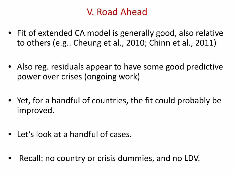
V. Road Ahead

• Fit of extended CA model is generally good, also relative to others (e.g.. Cheung et al., 2010; Chinn et al., 2011)

• Also reg. residuals appear to have some good predictive power over crises (ongoing work)

• Yet, for a handful of countries, the fit could probably be improved.

• Let’s look at a handful of cases.

• Recall: no country or crisis dummies, and no LDV.

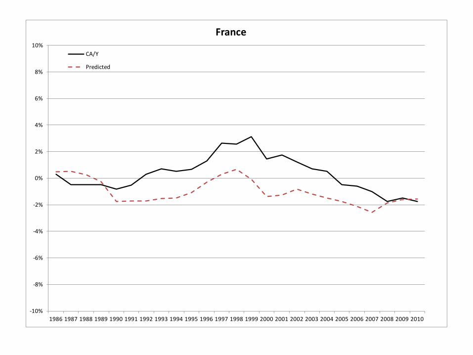
-10%

-8%

-6%

-4%

-2%

0%

2%

4%

6%

8%

10%

1986 1987 1988 1989 1990 1991 1992 1993 1994 1995 1996 1997 1998 1999 2000 2001 2002 2003 2004 2005 2006 2007 2008 2009 2010

France

CA/Y

Predicted

-15%

-10%

-5%

0%

5%

10%

1986 1987 1988 1989 1990 1991 1992 1993 1994 1995 1996 1997 1998 1999 2000 2001 2002 2003 2004 2005 2006 2007 2008 2009 2010

Spain

CA/Y

Predicted

Yet, a case where the fit deteriorates half-way

-4%

-2%

0%

2%

4%

6%

8%

1986 1987 1988 1989 1990 1991 1992 1993 1994 1995 1996 1997 1998 1999 2000 2001 2002 2003 2004 2005 2006 2007 2008 2009 2010

Germany

CA/Y

Predicted

• There are also cases where the mean fitted CA is substantially lower than actual CA throughout 1986-2010.

• The regression also tends to have a harder time in predicting the large (and sometimes long-lasting) current account surpluses that follow some financial crises, and crisis dummies seem to do a paltry job at that.

• But some good news even there: regression residuals do point to an over-valuation in the run-up to most (if not all) of these crises!

How about some “fixes”? • Adding the LDV is one and there is some theory in

support. But without fixed effects is problematic because soaks in FEs.

• On the other hand, adding the LDV with FE’s just throws the baby out with the water.

• So, the way to go seem to look for economically sensible quasi-fixed effects in some cases; and better controls for time variations in others.

• Post-financial crisis mis-fits do suggest that controls

for overshooting and undershooting of domestic credit may be an important future add-on.

• Other quasi-fixed effects may also be worth exploring given very long-run patterns.

• For instance, Germany’s century-long surpluses, Australia’s century-long deficits, etc.

Thanks.