CUMULATIVE ENVIRONMENTAL MANAGEMENT ASSOCIATION (CEMA)

Report Disclaimer This report was commissioned by the Cumulative Environmental Management Association (CEMA). This report has been completed in accordance with the Working Group’s terms of reference. The Working Group has closed this project and considers this report final. The Working Group does not fully endorse all of the contents of this report, nor does the report necessarily represent the views or opinions of CEMA or the CEMA Members. The conclusions and recommendations contained within this report are those of the consultant, and have neither been accepted nor rejected by the Working Group. Until such time as CEMA issues correspondence confirming acceptance, rejection, or non-consensus regarding the conclusions and recommendations contained in this report, they should be regarded as information only.

For more information please contact CEMA at 780-799-3947.

***All information contained within this report is owned and copyrighted by the Cumulative Environmental Management Association. As a user, you are granted a limited license to display or print the information provided for personal, non-commercial use only, provided the information is not modified and all copyright and other proprietary notices are retained. None of the information may be otherwise reproduced, republished or re-disseminated in any manner or form without the prior written permission of an authorized representative of the Cumulative Environmental Management Association.***

Cumulative Environmental Management Association Suite 214, 9914 Morrison Street

Fort McMurray, AB T9H 4A4 Phone: 780-799-3947

Facsimile: 780-714-3081 E-Mail: info@cemaonline.ca

Website: www.cemaonline.ca

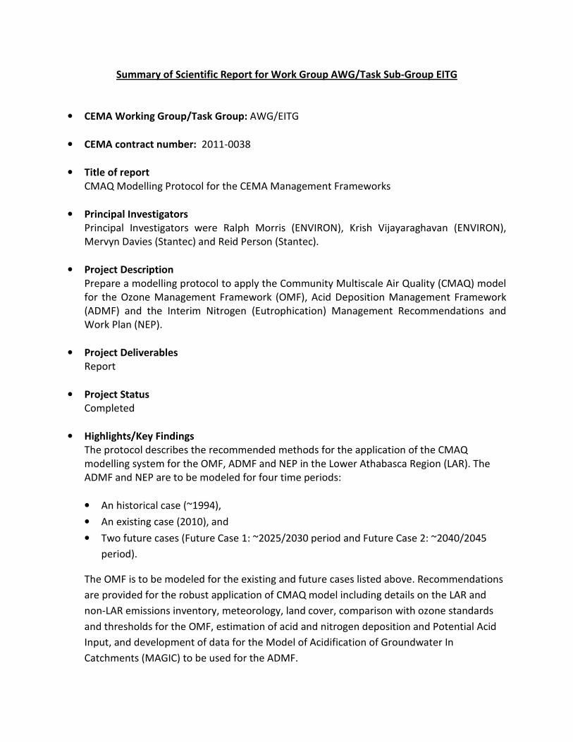
Summary of Scientific Report for Work Group AWG/Task Sub-Group EITG

• CEMA Working Group/Task Group: AWG/EITG

• CEMA contract number: 2011-0038

• Title of report

CMAQ Modelling Protocol for the CEMA Management Frameworks

• Principal Investigators

Principal Investigators were Ralph Morris (ENVIRON), Krish Vijayaraghavan (ENVIRON),

Mervyn Davies (Stantec) and Reid Person (Stantec).

• Project Description

Prepare a modelling protocol to apply the Community Multiscale Air Quality (CMAQ) model

for the Ozone Management Framework (OMF), Acid Deposition Management Framework

(ADMF) and the Interim Nitrogen (Eutrophication) Management Recommendations and

Work Plan (NEP).

• Project Deliverables

Report

• Project Status

Completed

• Highlights/Key Findings

The protocol describes the recommended methods for the application of the CMAQ

modelling system for the OMF, ADMF and NEP in the Lower Athabasca Region (LAR). The

ADMF and NEP are to be modeled for four time periods:

• An historical case (~1994),

• An existing case (2010), and

• Two future cases (Future Case 1: ~2025/2030 period and Future Case 2: ~2040/2045

period).

The OMF is to be modeled for the existing and future cases listed above. Recommendations

are provided for the robust application of CMAQ model including details on the LAR and

non-LAR emissions inventory, meteorology, land cover, comparison with ozone standards

and thresholds for the OMF, estimation of acid and nitrogen deposition and Potential Acid

Input, and development of data for the Model of Acidification of Groundwater In

Catchments (MAGIC) to be used for the ADMF.

773 San Marin Drive, Suite 2115, Novato, CA 94998, Phone: 415.899.0700

Final Report

CMAQ Modelling Protocol for the

CEMA Management Frameworks

Prepared for:

Cumulative Environmental Management Association -

Air Working Group

Morrison Center, Suite 214

9914 Morrison Street

Fort McMurray, AB T9H 4A4

Prepared by:

Krish Vijayaraghavan and Ralph Morris

ENVIRON International Corporation

773 San Marin Drive, Suite 2115

Novato, CA 94998

Mervyn Davies and Reid Person

Stantec Consulting Ltd.

300-805 8th Avenue SW

Calgary, AB T2P 1H7

June 2012

Environ CA12-00394A

Stantec 123559 (T220)

i

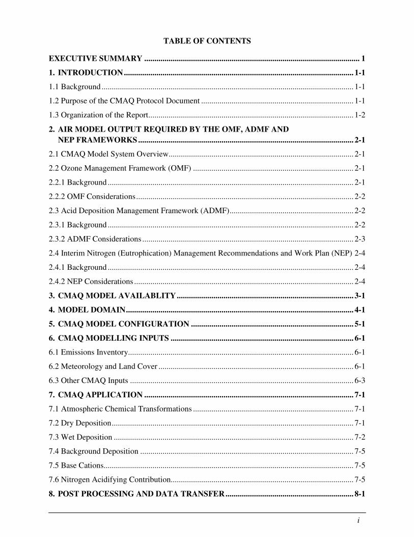
TABLE OF CONTENTS

EXECUTIVE SUMMARY .......................................................................................................... 1

1. INTRODUCTION ................................................................................................................. 1-1

1.1 Background ............................................................................................................................ 1-1

1.2 Purpose of the CMAQ Protocol Document ........................................................................... 1-1

1.3 Organization of the Report ..................................................................................................... 1-2

2. AIR MODEL OUTPUT REQUIRED BY THE OMF, ADMF AND

NEP FRAMEWORKS .......................................................................................................... 2-1

2.1 CMAQ Model System Overview........................................................................................... 2-1

2.2 Ozone Management Framework (OMF) ............................................................................... 2-1

2.2.1 Background ......................................................................................................................... 2-1

2.2.2 OMF Considerations ........................................................................................................... 2-2

2.3 Acid Deposition Management Framework (ADMF) ............................................................. 2-2

2.3.1 Background ......................................................................................................................... 2-2

2.3.2 ADMF Considerations ........................................................................................................ 2-3

2.4 Interim Nitrogen (Eutrophication) Management Recommendations and Work Plan (NEP) 2-4

2.4.1 Background ......................................................................................................................... 2-4

2.4.2 NEP Considerations ............................................................................................................ 2-4

3. CMAQ MODEL AVAILABLITY ....................................................................................... 3-1

4. MODEL DOMAIN ................................................................................................................ 4-1

5. CMAQ MODEL CONFIGURATION ................................................................................ 5-1

6. CMAQ MODELLING INPUTS .......................................................................................... 6-1

6.1 Emissions Inventory............................................................................................................... 6-1

6.2 Meteorology and Land Cover ................................................................................................ 6-1

6.3 Other CMAQ Inputs .............................................................................................................. 6-3

7. CMAQ APPLICATION ....................................................................................................... 7-1

7.1 Atmospheric Chemical Transformations ............................................................................... 7-1

7.2 Dry Deposition ....................................................................................................................... 7-1

7.3 Wet Deposition ...................................................................................................................... 7-2

7.4 Background Deposition ......................................................................................................... 7-5

7.5 Base Cations........................................................................................................................... 7-5

7.6 Nitrogen Acidifying Contribution.......................................................................................... 7-5

8. POST PROCESSING AND DATA TRANSFER ............................................................... 8-1

ii

8.1 OMF ....................................................................................................................................... 8-1

8.2 ADMF and NEP ..................................................................................................................... 8-2

9. COMPUTATIONAL REQUIREMENTS ........................................................................... 9-1

10. MODEL PERFORMANCE EVALUATION ............................................................ 10-1

10.1 Model Performance ............................................................................................................ 10-1

10.2 Model Harmonization Potential ......................................................................................... 10-1

11. REFERENCES ............................................................................................................. 11-1

LIST OF TABLES

Table 5-1. CMAQ model configuration for CEMA modelling .................................................. 5-2

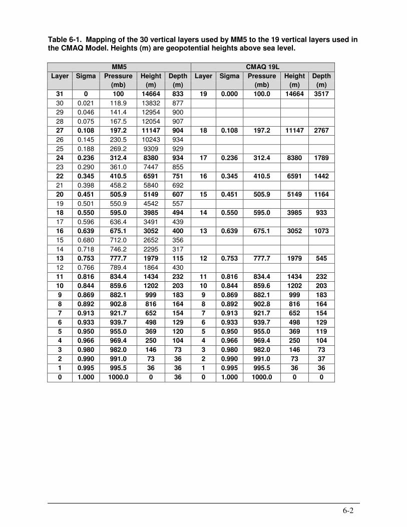
Table 6-1. Mapping of the 30 vertical layers used by MM5 to the 19 vertical layers used in the

CMAQ Model. Heights (m) are geopotential heights above sea level. ....................................... 6-2

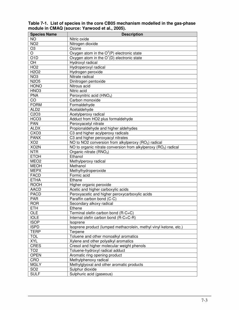
Table 7-1. List of species in the core CB05 mechanism modelled in the gas-phase module in

CMAQ (source: Yarwood et al., 2005). ....................................................................................... 7-3

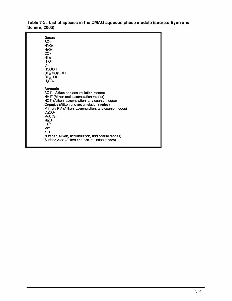
Table 7-2. List of species in the CMAQ aqueous phase module (source: Byun and Schere,

2006). ........................................................................................................................................... 7-4

Table A-1. Reactions and rate constants for the core CB05 mechanism used in the gas-phase

module in CMAQ (source: Yarwood et al., 2005).......................................................................... II

LIST OF FIGURES

Figure 4-1. CEMA CMAQ 36/12/4 km modelling domains 4-1

iii

LIST OF ABBREVIATIONS

ACMF Air Contaminants Management Framework

ADMF Acid Deposition Management Framework

AEW Alberta Environment and Water

AWG Air Working Group

CALMET California Meteorological Model Processor

CALPUFF California Puff Model

CEMA Cumulative Environmental Management Association

CMAQ Community Multiscale Air Quality Model

EC Environment Canada

HNO3 Nitric acid

H2SO4 Sulphuric acid

ISORROPIA Inorganic gas/aerosol partitioning model (Means equilibrium in Greek)

LAI Leaf Area Index

LAR Lower Athabasca Region

LARP Lower Athabasca Regional Plan

LICA Lakeland Industry and Community Association

MAGIC Model for Acidification of Groundwater in Catchments

NEP Interim Nitrogen (Eutrophication) Management Recommendations and Work

Plan

NH3 Ammonia

NO Nitric oxide

NO2 Nitrogen dioxide

NOX Nitrogen oxides (NO and NO2)

NO3- Nitrate ion

OMF Ozone Management Framework

PAI Potential acid input

RADM Regional Acid Deposition Model

RELAD Regional Lagrangian Acid Deposition Model

RMWB Regional Municipality of Wood Buffalo

SO2 Sulphur dioxide

SO42-

Sulphate ion

U.S. EPA United States Environmental Protection Agency

WBEA Wood Buffalo Environmental Association

1

EXECUTIVE SUMMARY

PROJECT OBJECTIVE

The Cumulative Environmental Management Association (CEMA), via the Air Working Group

(AWG) has developed an Ozone Management Framework, Acid Deposition Management

Framework (ADMF) and an Interim Nitrogen (Eutrophication) Management Recommendations

and Work Plan (NEP) for the Regional Municipality of Wood Buffalo (RMWB). The successful

implementation of the OMF, ADMF and the NEP requires ambient air quality and deposition

modelling to assess historical, current, and future environmental exposures due to emissions

from the oil sands industry and other sources in and around the RMWB.

Two air quality model systems, CALPUFF and CMAQ (the Community Multiscale Air Quality

Model) have been compared and reviewed for their appropriateness to address these CEMA

management frameworks (Vijayaraghavan et al 2011a, 2012). The comparison studies

recommended the application of the CMAQ model for the OMF but did not reach a conclusion

on the preferred model to provide deposition predictions for the ADMF and the NEP. This

document provides a protocol for the application of CMAQ for the OMF and ADMF/NEP based

on the assumption that CEMA applies CMAQ for the ADMF/NEP (instead of or in conjunction

with CALPUFF) in addition to the OMF.

MODEL APPLICATION PRINCIPLES

Applications of air quality simulation models for these frameworks should adhere to the

following two principles, namely:

1. Model input, assumptions, applications and comparisons need to be in public domain

documents to enhance and maintain the credibility of the information to external

stakeholders.

2. Common public domain information would enhance consistency for future

assessments undertaken for the region. Although we recognize that while consistency

is desirable, it should not preclude the continuing evolution and enhancement of

approaches.

These principles are consistent with the needs identified by others (e.g., Foster, 2010). The

overall goal of the protocol document is to facilitate the application of a scientifically defensible

model for the OMF, ADMF and the NEP.

EMISSION INVENTORY

The OMF requires the application of the CMAQ model system to three time periods: one current,

one 15 years in the future, and one 30 years in the future. The ADMF/NEP requires that CMAQ

be applied for a historical period in addition to these three time periods, resulting in a total of

four temporal scenarios (historical, existing, two future cases). Davies et al (2012a) documents

and provides a source and emission inventory for industrial and non-industrial sources located in

the Lower Athabasca Region (LAR) for the four time periods. An improved speciation profile

representing the fractions of individual compounds in oil sands volatile organic compounds

2

(VOC) emissions based on measurements is incorporated in the emissions inventory

(Nopmongcol et al., 2012). There are four different LAR industrial inventories, one for each of

the four time periods. There are two different LAR non-industrial inventories, one for the two

future cases and one for the historical/existing case. The inventories for industrial and non-

industrial sources located outside the LAR are described by Nopmongcol et al. (2012) and will

be held constant for all temporal cases.

METEOROLOGY AND LANDCOVER

Prognostic modelled fields from a model such as MM5, in particular, those for precipitation,

offer the advantage of higher density and capturing orographic variability compared to sparse

measurements in the region. A horizontal resolution of 4 km is required to capture variability

within the LAR. Dry deposition is strongly influenced by leaf area index (LAI) that varies with

vegetation canopy type and season. We will process 1980 and 2009/2010 MM5 meteorological

files provided by CEMA for the CMAQ background and 2009/2010 runs, respectively. We will

update the LAI input to CMAQ based on MODIS satellite data and utilize internal CMAQ

algorithms for computing dry deposition velocities based on the revised LAI. A sensitivity test

will be conducted (one week in summer and one week in winter) with the default and improved

LAI to determine the effect of using improved LAI on CMAQ outputs.

COMPARISON WITH OZONE STANDARDS AND THRESHOLDS

Spatial distributions of predicted concentrations of ozone in the LAR in the existing and two

future cases will be compared with local, provincial and national standards, with emphasis on

CEMA metrics. Chronic (3-month growing season) SUM60 ozone predictions in the RMWB

will be compared with the CEMA Baseline, Surveillance, Management and Exceedance levels.

Other metrics of interest include the Canada Wide Standards (CWS) for 8-hour ozone, acute (3-

day) and chronic SUM60 exposure levels from Health Canada and Environment Canada, the

chronic AOT40 threshold from UN/ECE and the W126 metric which is under consideration by

the AWG. The CMAQ predictions of the ozone precursors NO2 and CO will also be compared

with the Canada National Ambient Air Quality Objectives (NAAQOs) and Alberta Ambient Air

Quality Objectives (AAAQOs) and Ambient Air Quality Guidelines (AAAQGs) for 1-hour, 24-

hour and annual NO2 concentrations and 1-hour and 8-hour CO concentrations. CMAQ outputs

will also be compared with proposed standards under the new Air Quality Management System

(AQMS).

ACID DEPOSITION AND NITROGEN DEPOSITION

Spatial distributions of wet and dry deposition of sulphur and nitrogen compounds will be

analyzed. Modelled PAI will be compared to the Alberta critical, target, and monitoring

deposition loads in sensitive areas (0.25 keq/ha/a, 0.22 keq/ha/a and 0.17 keq/ha/a,

respectively).The temporal scale of interest relative to the ADMF and NEP is the annual acid

deposition and nitrogen deposition predicted by CMAQ. In addition to a floating 4 by 4

township/range (39 by 39 km) block specific to the ADMF, annual CMAQ deposition

predictions at selected grid 4 km x 4 km grid cells corresponding to lakes and other receptors of

interest will be available for use in the Model for Acidification of Groundwater in Catchments

3

(MAGIC) that is used to assess responses in water quality. We will continue to use the base

cation contributions based on earlier work by Alberta Environment and Water (AEW).

CLOSING

CMAQ offers the advantage of application of state-of-the-science chemistry in both the OMF

and the ADMF/NEP and the ability to model the contributions of sources both inside and outside

the LAR. Following the recommendations provided in this protocol will enhance the credibility

of the model predictions in the context of the CEMA management frameworks.

1-1

1. INTRODUCTION

1.1 BACKGROUND

The Cumulative Environmental Management Association (CEMA) is a multi‐stakeholder

organization that facilitates consensus-based decisions forming the basis for action by members

and provides recommendations to Alberta Environment’s Regional Sustainable Development

Strategy (RSDS) to address the cumulative effects of development within the Regional

Municipality of Wood Buffalo (RMWB). A number of Working Groups have been established

within CEMA to address specific health and environmental issues associated with industrial

development in the RMWB. One of these Groups, the NOX and SO2 Management Working

Group (NSMWG) was mandated to develop and recommend management plans (frameworks)

for oxides of nitrogen (NOX) and sulphur dioxide (SO2) emissions as they relate to acid

deposition, nitrogen deposition and ground level ozone (O3). The Trace Metals and Air

Contaminants (TMAC) Working Group was established to develop management frameworks to

manage and control regional trace metals and air contaminants and protect human and ecosystem

health. The Air Working Group (AWG) was established to adopt work in progress initiated by

these earlier working groups and initiate new work as required.

In accordance with their mandates, NSMWG and TMAC have developed the following

management framework/plan documents:

• Acid Deposition Management Framework (ADMF)

• Ozone Management Framework (OMF)

• Interim Nitrogen (Eutrophication) Management Recommendations and Work Plan (NEP)

• Air Contaminants Management Framework (ACMF)

Implementation of these frameworks/plans relies to varying degrees on ambient air quality and

deposition modelling to assess environmental exposure to airborne and deposited substances

emitted from the oil sands industry and other sources in and around the RMWB. CEMA initiated

a multi-phase emissions inventory and air quality modelling study that builds upon prior work

supported by CEMA and other organizations and is designed to facilitate the implementation of

the management frameworks by leveraging their common features.

1.2 PURPOSE OF THE CMAQ PROTOCOL DOCUMENT

Two air quality model systems, CALPUFF and CMAQ (the Community Multiscale Air Quality

Model) have been compared and reviewed for their appropriateness to address these CEMA

management frameworks (Vijayaraghavan et al. 2011a, 2012). The comparison studies

recommended the application of the CMAQ model for the OMF but did not reach a conclusion

on the preferred model to provide deposition predictions for the ADMF and the NEP. This

document provides a protocol for the application of CMAQ for the OMF and ADMF/NEP based

on the assumption that CEMA applies CMAQ for the OMF and for the ADMF/NEP (instead of

or in conjunction with CALPUFF).

1-2

1.3 ORGANIZATION OF THE REPORT

The report is organized as follows:

• Section 1 (this Section) presents an introduction and overview of the study.

• Section 2 discusses how CMAQ will be used to meet the needs of the OMF, ADMF and

NEP.

• Section 3 discusses the availability of the CMAQ model system.

• Section 4 outlines the proposed model domain.

• Section 5 outlines the proposed CMAQ configuration.

• Section 6 outlines meteorology and other modelling inputs.

• Section 7 describes some key components of the CMAQ applications

• Section 8 discusses the comparison of CMAQ predictions with ozone metrics for the

OMF, the processing of CMAQ outputs for the ADMF and NEP and the transfer of the

CMAQ model output to terrestrial and aquatic disciplines.

• Section 9 lists typical computational requirements relating to the application of the

CMAQ model.

• Section 10 discusses the proposed CMAQ model performance evaluation.

2-1

2. AIR MODEL OUTPUT REQUIRED BY THE OMF, ADMF AND NEP

FRAMEWORKS

In this section, we describe how the modelling needs of the OMF, ADMF and NEP will be met

by application of the CMAQ model system.

2.1 CMAQ MODEL SYSTEM OVERVIEW

CMAQ is a three-dimensional Eulerian photochemical chemical transport model, also called a

photochemical grid model (PGM), that includes state-of-the-science capabilities for modelling

multiple air quality issues, including tropospheric ozone, acid deposition, nitrogen deposition,

fine particles, other air contaminants, and visibility degradation (Byun and Schere, 2006; Foley

et al., 2010). CMAQ is part of an advanced modelling system (Models-3) that also includes a

meteorological pre-processor (MCIP), initial and boundary conditions processors (ICON and

BCON), a photolysis rates processor (JPROC), and an emissions model (SMOKE) to develop

CMAQ-ready emissions from anthropogenic and natural emissions inventories. Models-3 also

includes utilities (known as the M3 I/O library) and other graphics software to process CMAQ

input and output files.

There is no single photochemical grid model recommended by the EPA for regulatory

applications. However, CMAQ is one of the most commonly-used photochemical grid models

and is applied routinely by the EPA to support rule-making and by state agencies and industry to

implement or analyze those rules. CMAQ has been applied recently in Alberta and the Lower

Athabasca Region (LAR) (Fox and Kellerhals, 2007; Morris et al., 2010a, 2010b; Cho et al.,

2012a, 2012b) to support PM and ozone chemistry modelling.

2.2 OZONE MANAGEMENT FRAMEWORK (OMF)

2.2.1 Background

The focus of the OMF is to understand and manage the photochemical production of ozone in the

LAR due to LAR precursor NOX and VOC emission sources. Other potential sources of elevated

ozone concentration in the LAR include: the long-range transport of photochemically produced

ozone from upwind precursor anthropogenic and biogenic sources (e.g., the Edmonton region),

the formation of ozone in the LAR from precursors outside the LAR, the downward mixing of

ozone rich stratospheric air by continuous stratosphere-troposphere air exchange processes or by

discrete stratospheric intrusions, and by photochemical production due to precursor emissions

from biomass burning (e.g., wild fires).

The CMAQ model has been applied to predict ambient ozone levels in Alberta. Environment

Canada (Fox and Kellerhals, 2007) examined the summer period June to August inclusive to

focus on the photochemical production of ozone in the LAR due to anthropogenic precursor NOX

and VOC emission sources. In contrast, the CEMA study (Morris et al., 2010a) simulated a full

year, 2006 at 36/12 km horizontal resolution, as this facilitated simultaneous study of acid

deposition and other contaminants such as PM2.5 which are important throughout the year in

2-2

addition to ozone. Cho et al. (2012a, 2012b) studied ozone and PM using CMAQ at a finer

horizontal resolution (4 km) during May-August 2002 in northeastern Alberta.

2.2.2 OMF Considerations

The OMF requires predictions of ground-level hourly average ozone concentrations. The hourly

data from CMAQ allow various ozone metrics to be calculated (e.g., the highest 8-hour rolling

average in each 24 hour period as per the Canada Wide Standards (CWS), the SUMxx metric that

is the sum of the concentrations that exceed xx during daylight hours, the AOTxx metric that is

the sum of the positive differences between hourly values and the xx threshold, or the W126

metric under consideration that is a cumulative peak-weighted index). The preferred

concentration units for these calculations are in units of parts per billion (ppb) by volume and the

metrics are reported in ppb-hours.

For the OMF, the seasonal and diurnal temporal variations of the precursor emission rates are

important to resolve. To understand the photochemical contribution associated with the LAR

precursor emissions, the focus of the modelling is typically on the summer May to August

period. However, to allow for the results of the CMAQ application to be potentially useful for

other CEMA management frameworks, we recommend that CMAQ be applied on an annual

basis rather than just for the summer season.

The OMF does not identify a spatial scale. However a resolution of 4 km should be sufficient to

address the needs of the OMF as ozone is a regional issue.

2.3 ACID DEPOSITION MANAGEMENT FRAMEWORK (ADMF)

2.3.1 Background

Because acidification occurs slowly, and the consequent ecological response occurs even more

slowly, the ADMF uses early indications of chemical change in soil and lakes rather than waiting

for ecological change to occur. As the chemical change in soil and lakes is often directly related

to changes in atmospheric deposition, the framework uses predictions of atmospheric deposition

and Potential Acid Input (PAI) to detect exceedances of the monitoring, target and critical loads

and to predict the response in atmospheric deposition to anticipated changes in regional

emissions.

PAI is derived from the acid and base cation deposition fluxes as the total sulphur compound

contribution (PAI[sulphur]) plus the total nitrogen compound contribution (PAI[nitrogen]) minus

the neutralizing effect of base cations (PAI[base cation]). The PAI values (expressed in units of

keq H+/ha/) are calculated as follows using CMAQ modelled deposition values:

���������� =1

30��� +

1

46���� +

2

108����� +

1

47����� +

1

63����� +

1

79�����

+1

62����

����!"#$ℎ" =2

64�&�� +

2

96�&��

�

2-3

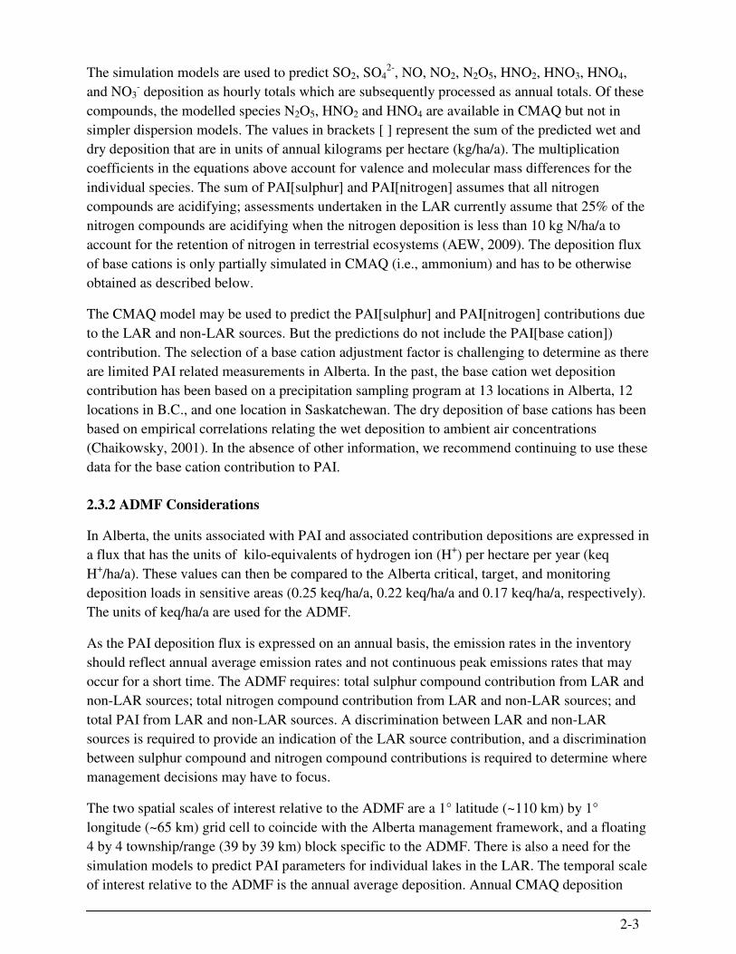
The simulation models are used to predict SO2, SO42-

, NO, NO2, N2O5, HNO2, HNO3, HNO4,

and NO3- deposition as hourly totals which are subsequently processed as annual totals. Of these

compounds, the modelled species N2O5, HNO2 and HNO4 are available in CMAQ but not in

simpler dispersion models. The values in brackets [ ] represent the sum of the predicted wet and

dry deposition that are in units of annual kilograms per hectare (kg/ha/a). The multiplication

coefficients in the equations above account for valence and molecular mass differences for the

individual species. The sum of PAI[sulphur] and PAI[nitrogen] assumes that all nitrogen

compounds are acidifying; assessments undertaken in the LAR currently assume that 25% of the

nitrogen compounds are acidifying when the nitrogen deposition is less than 10 kg N/ha/a to

account for the retention of nitrogen in terrestrial ecosystems (AEW, 2009). The deposition flux

of base cations is only partially simulated in CMAQ (i.e., ammonium) and has to be otherwise

obtained as described below.

The CMAQ model may be used to predict the PAI[sulphur] and PAI[nitrogen] contributions due

to the LAR and non-LAR sources. But the predictions do not include the PAI[base cation])

contribution. The selection of a base cation adjustment factor is challenging to determine as there

are limited PAI related measurements in Alberta. In the past, the base cation wet deposition

contribution has been based on a precipitation sampling program at 13 locations in Alberta, 12

locations in B.C., and one location in Saskatchewan. The dry deposition of base cations has been

based on empirical correlations relating the wet deposition to ambient air concentrations

(Chaikowsky, 2001). In the absence of other information, we recommend continuing to use these

data for the base cation contribution to PAI.

2.3.2 ADMF Considerations

In Alberta, the units associated with PAI and associated contribution depositions are expressed in

a flux that has the units of kilo-equivalents of hydrogen ion (H+) per hectare per year (keq

H+/ha/a). These values can then be compared to the Alberta critical, target, and monitoring

deposition loads in sensitive areas (0.25 keq/ha/a, 0.22 keq/ha/a and 0.17 keq/ha/a, respectively).

The units of keq/ha/a are used for the ADMF.

As the PAI deposition flux is expressed on an annual basis, the emission rates in the inventory

should reflect annual average emission rates and not continuous peak emissions rates that may

occur for a short time. The ADMF requires: total sulphur compound contribution from LAR and

non-LAR sources; total nitrogen compound contribution from LAR and non-LAR sources; and

total PAI from LAR and non-LAR sources. A discrimination between LAR and non-LAR

sources is required to provide an indication of the LAR source contribution, and a discrimination

between sulphur compound and nitrogen compound contributions is required to determine where

management decisions may have to focus.

The two spatial scales of interest relative to the ADMF are a 1° latitude (~110 km) by 1°

longitude (~65 km) grid cell to coincide with the Alberta management framework, and a floating

4 by 4 township/range (39 by 39 km) block specific to the ADMF. There is also a need for the

simulation models to predict PAI parameters for individual lakes in the LAR. The temporal scale

of interest relative to the ADMF is the annual average deposition. Annual CMAQ deposition

2-4

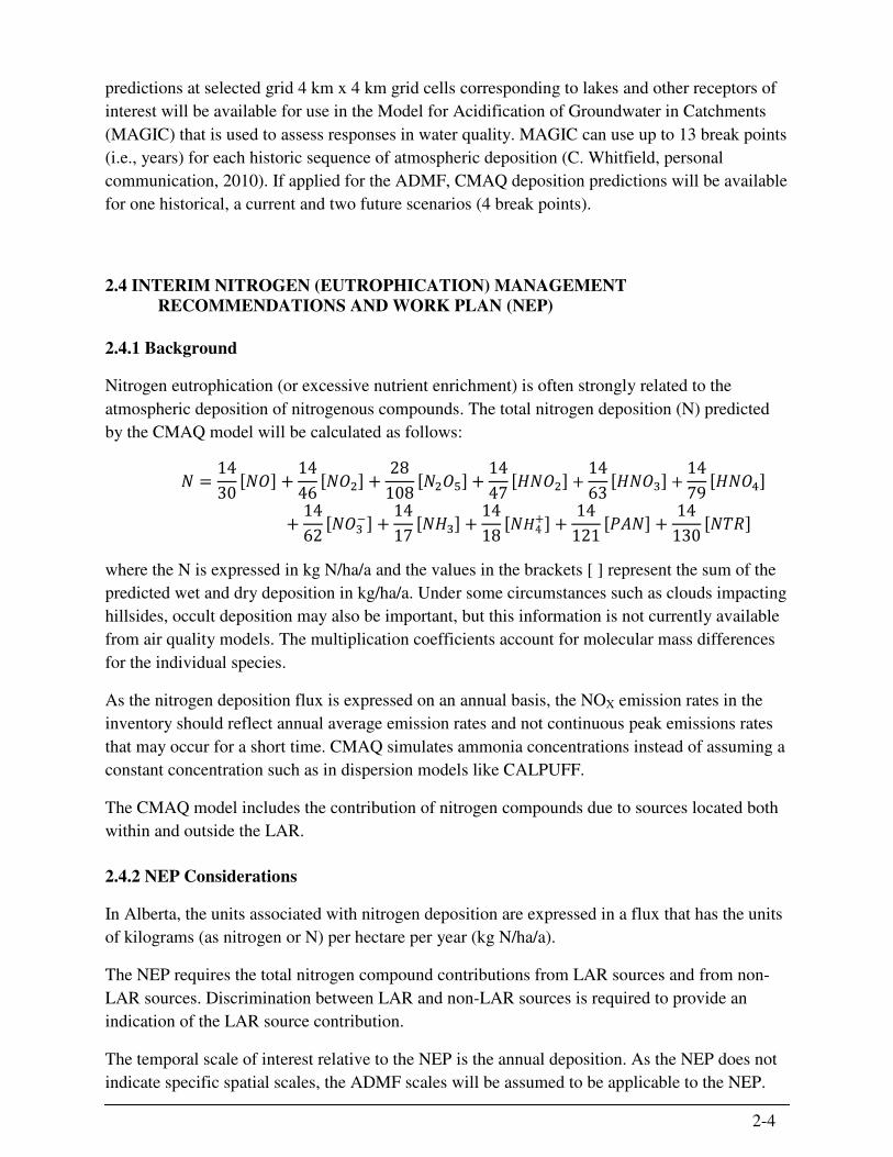
predictions at selected grid 4 km x 4 km grid cells corresponding to lakes and other receptors of

interest will be available for use in the Model for Acidification of Groundwater in Catchments

(MAGIC) that is used to assess responses in water quality. MAGIC can use up to 13 break points

(i.e., years) for each historic sequence of atmospheric deposition (C. Whitfield, personal

communication, 2010). If applied for the ADMF, CMAQ deposition predictions will be available

for one historical, a current and two future scenarios (4 break points).

2.4 INTERIM NITROGEN (EUTROPHICATION) MANAGEMENT

RECOMMENDATIONS AND WORK PLAN (NEP)

2.4.1 Background

Nitrogen eutrophication (or excessive nutrient enrichment) is often strongly related to the

atmospheric deposition of nitrogenous compounds. The total nitrogen deposition (N) predicted

by the CMAQ model will be calculated as follows:

� =14

30��� +

14

46���� +

28

108����� +

14

47����� +

14

63����� +

14

79�����

+14

62����

+14

17���� +

14

18���4

+ +14

121���� +

14

130��'(

where the N is expressed in kg N/ha/a and the values in the brackets [ ] represent the sum of the

predicted wet and dry deposition in kg/ha/a. Under some circumstances such as clouds impacting

hillsides, occult deposition may also be important, but this information is not currently available

from air quality models. The multiplication coefficients account for molecular mass differences

for the individual species.

As the nitrogen deposition flux is expressed on an annual basis, the NOX emission rates in the

inventory should reflect annual average emission rates and not continuous peak emissions rates

that may occur for a short time. CMAQ simulates ammonia concentrations instead of assuming a

constant concentration such as in dispersion models like CALPUFF.

The CMAQ model includes the contribution of nitrogen compounds due to sources located both

within and outside the LAR.

2.4.2 NEP Considerations

In Alberta, the units associated with nitrogen deposition are expressed in a flux that has the units

of kilograms (as nitrogen or N) per hectare per year (kg N/ha/a).

The NEP requires the total nitrogen compound contributions from LAR sources and from non-

LAR sources. Discrimination between LAR and non-LAR sources is required to provide an

indication of the LAR source contribution.

The temporal scale of interest relative to the NEP is the annual deposition. As the NEP does not

indicate specific spatial scales, the ADMF scales will be assumed to be applicable to the NEP.

2-5

There is also a need for the simulation models to predict nitrogen deposition for selected lakes or

wetlands in the LAR. These will be determined in a manner similar to that described for the

ADMF.

3-1

3. CMAQ MODEL AVAILABLITY

EPA developed the CMAQ modelling system for public release in 1999 and has since revised it

frequently to incorporate new science algorithms and developments in model infrastructure.

CMAQ upgrades are made available to the public at no cost. CMAQ updates are made by the

Atmospheric Modelling and Analysis Division at EPA and released periodically (typically every

two years) by the Community Model and Analysis System (CMAS) Center at the University of

North Carolina Chapel Hill. The public releases include model code, preprocessors,

postprocessors, model documentation and test applications, all of which are available from the

CMAQ website (http://www.cmaq-model.org). CMAS also offers training courses on CMAQ

and associated processors, for a fee, in conjunction with the CMAS conference hosted annually

(http://www.cmascenter.org). In addition to formal support from CMAS, there is also an active

end-user community that assists in CMAQ-related trouble-shooting. The current version of

CMAQ is v.5.0 that was released in January 2012. CMAQ 5.0 offers several enhancements

compared to v 4.7.1 including gas-phase and aerosol chemistry and transport as described in the

CMAQ Release Notes (http://www.cmaq-model.org/ cmaqwiki/index.php?

title=CMAQ_version_5.0_%28February_2012_release%29_Technical_Documentation)

Recommendation: The current version of CMAQ (v 5.0) has been only recently released and

will undergo revisions as feedback on errors and model improvements is received from the

modelling community. However, because it combines current knowledge in atmospheric science

and air quality modelling, we still recommend this version for application to the OMF, ADMF

and NEP. If significant issues are experienced during the CEMA application due to the use of

this relatively untested code, we recommend switching to the prior version (v4.7.1).

4-1

4. MODEL DOMAIN

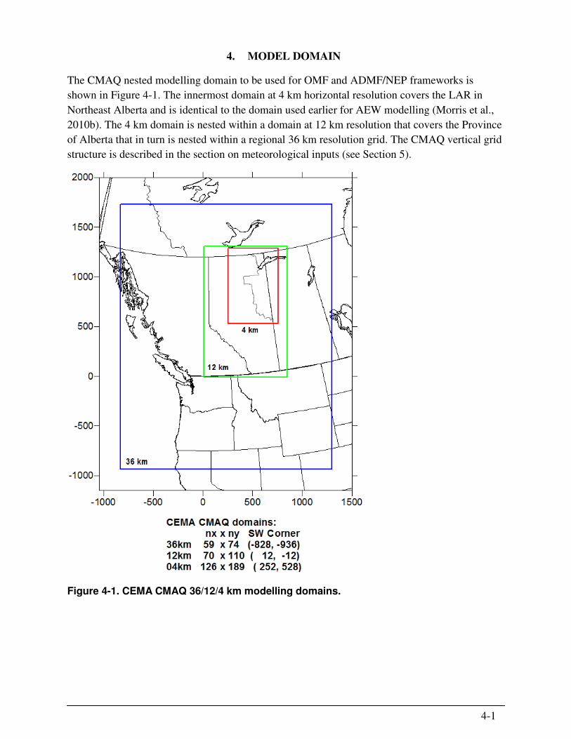
The CMAQ nested modelling domain to be used for OMF and ADMF/NEP frameworks is

shown in Figure 4-1. The innermost domain at 4 km horizontal resolution covers the LAR in

Northeast Alberta and is identical to the domain used earlier for AEW modelling (Morris et al.,

2010b). The 4 km domain is nested within a domain at 12 km resolution that covers the Province

of Alberta that in turn is nested within a regional 36 km resolution grid. The CMAQ vertical grid

structure is described in the section on meteorological inputs (see Section 5).

Figure 4-1. CEMA CMAQ 36/12/4 km modelling domains.

5-1

5. CMAQ MODEL CONFIGURATION

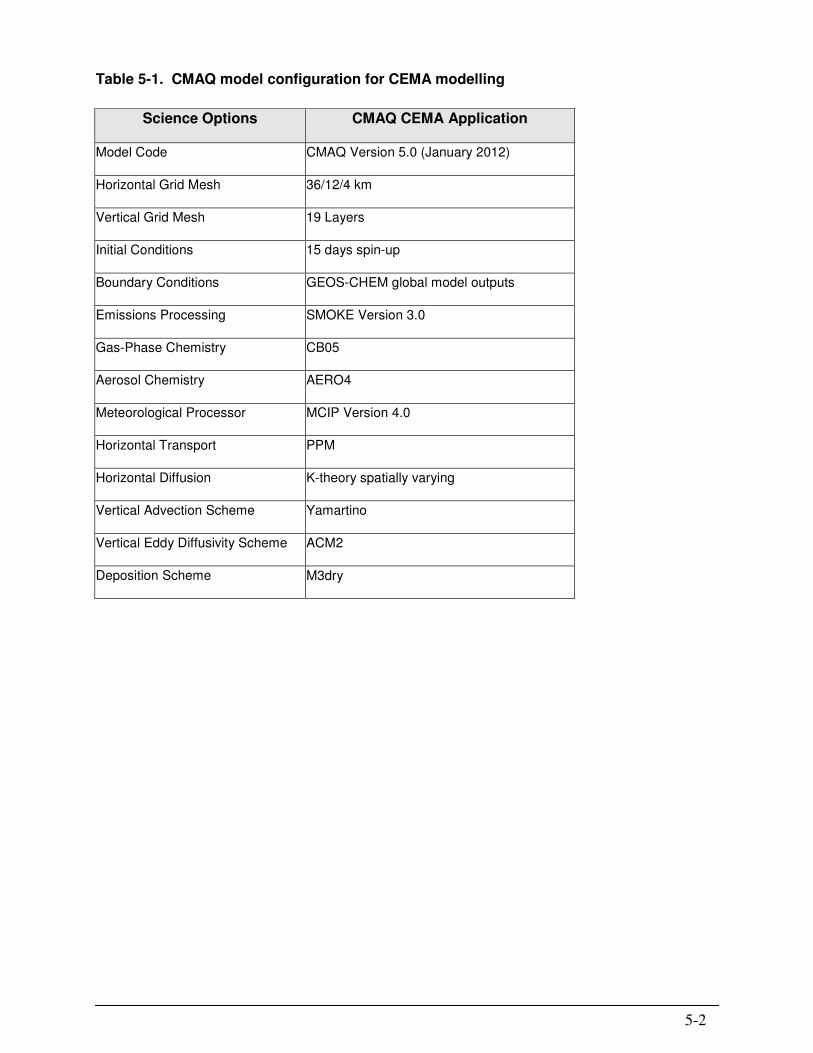
The proposed CMAQ model configuration is summarized in Table 5-1. The CMAQ CEMA

modelling database will be based on the following components:

• CMAQ Version 5.0 (version 4.7.1 will be used if unresolvable issues are identified in

version 5.0; the latter has new code that has not yet undergone rigorous testing by the air

quality modelling community)

• 19 pressure-based vertical levels with varying thicknesses from the surface to the

tropopause (see Section 6)

• Model spin-up of 15 days to mitigate the effect of initial conditions

• Boundary conditions of precursors of ozone, PM and acid deposition for the 36 km

domain from GEOS-Chem global model outputs (see Section 6)

• SMOKE Version 3.0 emissions modelling system (see Section 6)

• Carbon Bond 05 (CB05) photochemical mechanism

• Incorporation of the CB05 VOC speciation profile for oil sands VOC emissions in the

SMOKE emissions modelling (described in Nopmongcol et al., 2012)

• Aero4 aerosol mechanism

• MCIP Version 4.0 processing of MM5 meteorological data

• Piecewise parabolic method (PPM) for horizontal advection and K-theory for horizontal

diffusion (default methods in CMAQ)

• Yamartino scheme for vertical advection and the Asymmetric Convective Method

(ACM2) for vertical diffusion (default methods in CMAQ)

• M3DRY (Models-3 Dry) deposition scheme

5-2

Table 5-1. CMAQ model configuration for CEMA modelling

Science Options CMAQ CEMA Application

Model Code CMAQ Version 5.0 (January 2012)

Horizontal Grid Mesh 36/12/4 km

Vertical Grid Mesh 19 Layers

Initial Conditions 15 days spin-up

Boundary Conditions GEOS-CHEM global model outputs

Emissions Processing SMOKE Version 3.0

Gas-Phase Chemistry CB05

Aerosol Chemistry AERO4

Meteorological Processor MCIP Version 4.0

Horizontal Transport PPM

Horizontal Diffusion K-theory spatially varying

Vertical Advection Scheme Yamartino

Vertical Eddy Diffusivity Scheme ACM2

Deposition Scheme M3dry

6-1

6. CMAQ MODELLING INPUTS

6.1 EMISSIONS INVENTORY

CMAQ can simulate the contribution of emissions sources both inside and outside the LAR to

ozone, acid deposition and nitrogen deposition as required by the OMF, ADMF and NEP. The

emissions inventory to be used in CMAQ for the LAR is presented and discussed in the

document “Lower Athabasca Region Source and Emission Inventory” (Davies et al., 2012a). The

emissions inventory to be used in CMAQ for sources outside the LAR (both anthropogenic and

biogenic) as well as the processing of the LAR and non-LAR inventory using the Sparse Matrix

Operator Kernel Emissions (SMOKE) modelling system to perform chemical speciation, spatial

allocation and temporal allocation to develop CMAQ-ready emissions are discussed in the

document “Emissions Source Inventory outside Lower Athabasca Region and CMAQ Emissions

Modelling of Sources Inside and Outside the Region to Support CEMA Management

Frameworks” (Nopmongcol et al., 2012).

CMAQ is a multi-pollutant model and hence, the same model-ready emissions may be used for

the OMF and ADMF/NEP. However, only three temporal scenarios are required for the OMF

(the existing case and two future cases) while four scenarios are required for the ADMF/NEP (a

historical case in addition to the other three cases).

6.2 METEOROLOGY AND LAND COVER

The CMAQ application requires hourly meteorology over the 36/12/4 km resolution domains

shown in Figure 4-1. As advised by CEMA, we use 1980 meteorology for a “background”

CMAQ run and 2009/2010 meteorology for the modelling with 2009/2010 LAR emissions. The

1980 and 2009/2010 outputs from the Fifth Generation Mesoscale Model (MM5) (Grell et al.,

1994) will be provided by CEMA. Version 4.0 of the Meteorology-Chemistry Interface

Processor (MCIP) (Otte and Pleim, 2010) will be used to process these MM5 outputs and create

CMAQ-ready meteorological files for the CEMA modelling domain. MCIP reads MM5 fields,

performs horizontal and vertical coordinate transformations, calculates additional atmospheric

fields such as cloud liquid water content in a grid cell, defines gridding parameters, and prepares

the meteorological fields in the Network Common Data Form (netCDF) Input/Output

Applications Programming Interface (I/O API) format used by CMAQ. MCIP will be used to

collapse the 30 vertical layers used by MM5 meteorological model into 19 vertical layers for

CMAQ for computational efficiency, as shown in Table 6-1. The CMAQ 19 vertical layers

exactly match those used in the MM5 simulation for the lowest 11 vertical layers (up to ~1,400

m) closest to the surface. Thus, no layer collapsing between MM5 and CMAQ is employed

between the ground and approximately 1,400 m above ground level.

Additional modifications for the current CEMA modelling study are:

• If the annual meteorological fields provided by CEMA are available only at 36/12 km

horizontal resolutions, meteorology over the 12 km grid will be downscaled to 4 km

resolution over the spatial extent of the nested 4 km grid shown in Figure 4-1.

6-2

Table 6-1. Mapping of the 30 vertical layers used by MM5 to the 19 vertical layers used in the CMAQ Model. Heights (m) are geopotential heights above sea level.

MM5 CMAQ 19L

Layer Sigma Pressure Height Depth Layer Sigma Pressure Height Depth

(mb) (m) (m) (mb) (m) (m)

31 0 100 14664 833 19 0.000 100.0 14664 3517

30 0.021 118.9 13832 877

29 0.046 141.4 12954 900

28 0.075 167.5 12054 907

27 0.108 197.2 11147 904 18 0.108 197.2 11147 2767

26 0.145 230.5 10243 934

25 0.188 269.2 9309 929

24 0.236 312.4 8380 934 17 0.236 312.4 8380 1789

23 0.290 361.0 7447 855

22 0.345 410.5 6591 751 16 0.345 410.5 6591 1442

21 0.398 458.2 5840 692

20 0.451 505.9 5149 607 15 0.451 505.9 5149 1164

19 0.501 550.9 4542 557

18 0.550 595.0 3985 494 14 0.550 595.0 3985 933

17 0.596 636.4 3491 439

16 0.639 675.1 3052 400 13 0.639 675.1 3052 1073

15 0.680 712.0 2652 356

14 0.718 746.2 2295 317

13 0.753 777.7 1979 115 12 0.753 777.7 1979 545

12 0.766 789.4 1864 430

11 0.816 834.4 1434 232 11 0.816 834.4 1434 232

10 0.844 859.6 1202 203 10 0.844 859.6 1202 203

9 0.869 882.1 999 183 9 0.869 882.1 999 183

8 0.892 902.8 816 164 8 0.892 902.8 816 164

7 0.913 921.7 652 154 7 0.913 921.7 652 154

6 0.933 939.7 498 129 6 0.933 939.7 498 129

5 0.950 955.0 369 120 5 0.950 955.0 369 119

4 0.966 969.4 250 104 4 0.966 969.4 250 104

3 0.980 982.0 146 73 3 0.980 982.0 146 73

2 0.990 991.0 73 36 2 0.990 991.0 73 37

1 0.995 995.5 36 36 1 0.995 995.5 36 36

0 1.000 1000.0 0 36 0 1.000 1000.0 0 0

6-3

• Dry deposition is strongly influenced by leaf area index (LAI) that varies with vegetation

canopy type and season. The CMAQ LAI values from MM5 appear to be overestimated

in both winter and summer in the LAR (Vijayaraghavan et al., 2012). We will update the

LAI based on MODIS satellite data (https://lpdaac.usgs.gov/products/

modis_products_table/leaf_area_index_fraction_of_photosynthetically_active_radiation/

8_day_l4_global_1km/mod15a2) and further increase satellite LAI values over

coniferous areas by a factor of two to account for the uptake of gases by all sides of the

coniferous needles (Bourque and Hassan, 2008, 2010). We will utilize the M3Dry

algorithm in CMAQ to compute inline dry deposition velocities based on the LAI input to

CMAQ. A sensitivity test will be conducted (one week in summer and one week in

winter) with the default and improved LAI to determine the effect of using improved LAI

on CMAQ outputs.

6.3 OTHER CMAQ INPUTS

CMAQ requires boundary conditions (BC) inputs to specify the assumed concentrations along

the outer lateral edges of the 36 km modelling domain (see Figure 4-1) to account for the effect

of sources outside the domain on ozone and acid/nitrogen deposition in the LAR. The BCs for

the 12 km Alberta CMAQ modelling domain will be obtained by processing the CMAQ 36 km

domain output using the CMAQ BCON processor to generate an hourly 12 km BC input file.

Similarly, BCs for the inner 4 km domain will be obtained by processing the CMAQ 12 km

domain outputs.

The prior CEMA CMAQ modelling effort used BCs derived from a combination of 2002 GEOS-

Chem simulation outputs for winter and 2006 GEOS-Chem outputs for summer due to

availability constraints. In the current study, we will process 2006 GEOS-Chem outputs for all of

2006 to develop boundary conditions for the CMAQ 36 km domain. The 2006 GEOS-Chem year

is chosen as these outputs are readily available.

The GEOS-CHEM output will be processed by mapping the GEOS-CHEM chemical compounds

to the species in the CB05 chemical mechanism used by CMAQ and mapping the GEOS-CHEM

vertical layers to the 19 layer vertical layer structure used by CMAQ in the 36 km CEMA

modelling domain. The result will be day-specific three-hourly BC inputs for the CMAQ model

and the 36 km domain (See Figure 4-1) for all of 2006.

The initial conditions (ICs) for the CMAQ simulations will also be derived from 2006 GEOS-

Chem simulation outputs.

The same BCs and ICs will be used for all CMAQ scenarios.

7-1

7. CMAQ APPLICATION

The following subsections describe some key components of the CMAQ application and provide

recommendations relative to the OMF, ADMF and NEP.

7.1 ATMOSPHERIC CHEMICAL TRANSFORMATIONS

We will use the CB05 gas-phase chemical mechanism in CMAQ together with a modal

particulate matter size distribution algorithm and an aqueous chemistry model derived from the

Regional Acid Deposition Model (RADM) (Chang et al., 1987).

CMAQ has several advanced features for characterization of atmospheric deposition and ozone

and PM2.5 formation. For example, it includes a parameterization for heterogeneous (i.e., on

particle surfaces) conversion of N2O5 to PM2.5 nitrate. This reaction is enhanced at night-time

and can contribute to night-time nitrogen deposition. More details on the advanced chemistry

features in CMAQ may be found in the literature (e.g., Byun and Schere, 2006; Foley et al.,

2010). Table 7-1 lists the chemical compounds (species) that will be simulated in the gas-phase

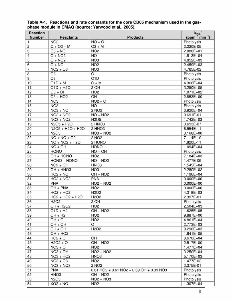
in CMAQ modelling for the OMF and ADMF/NEP. Table A-1 in the Appendix lists the

atmospheric gas-phase chemical transformations to be modelled. Table 7-2 lists the compounds

that will be simulated in the aqueous-phase in the CMAQ applications. The CB05 mechanism to

be used for gas-phase chemistry is a complex chemical mechanism. The core CB05 mechanism

has 51 species and 156 reactions as shown in Tables 7-1 and A-1. In addition to all the sulphur

and nitrogen compounds shown in Table 7-1, ammonia is also modelled in CMAQ; it

participates in aqueous-phase chemistry and partitioning to the particulate phase but does not

experience any gas-phase chemical transformations. The aqueous-phase module (see Table 7-2)

simulates 11 gases and 13 aerosol species or parameters.

In CMAQ, the particle size distribution is specified in three lognormal modal size distributions:

Aitken, accumulation and coarse modes (see Table 7-2 for a list of modelled compounds). The

first two roughly represent PM2.5 (fine PM) and the last one approximately PM10-2.5 (coarse PM).

Within the fine group, the Aitken mode represents fresh particles either from nucleation or from

direct emission, while the larger (accumulation) represents aged particles (Binkowski et al.,

1999). The two modes interact with each other through coagulation (i.e., particles sticking to

each other). Each mode may also grow through condensation of gaseous precursors; each mode

is subject to wet and dry deposition. Also, the smaller mode may grow into the larger mode and

partially merge with it. These PM size treatment processes in CMAQ are important for the

CEMA Management Frameworks because the magnitude of particulate nitrate, ammonium and

sulphate deposition depend on the PM size distribution.

7.2 DRY DEPOSITION

CMAQ uses a resistance model (comprising surface resistance, canopy resistance, and stomatal

resistance) to calculate dry deposition rates of gases and particulate matter. Dry deposition

velocity calculations are currently performed in MCIP but will be moved to within the CMAQ

code exclusively in the next release of CMAQ. The dry deposition process is simulated in

7-2

CMAQ (in a routine called M3DRY) as a flux boundary condition that affects the concentration

in the lowest vertical model layer.

7.3 WET DEPOSITION

We will utilize the aqueous-phase chemistry module in CMAQ based on RADM to calculate

aqueous-phase concentrations and wet deposition in precipitation. For those pollutants that are

absorbed into the cloud water and participate in the cloud chemistry, the amount of pollutant

scavenging depends on Henry's law constants, dissociation constants, and cloud water pH (Byun

and Schere, 2006). For pollutants that do not participate in aqueous chemistry, the model uses the

effective Henry's Law equilibrium equation to calculate ending concentrations and deposition

amounts.

7-3

Table 7-1. List of species in the core CB05 mechanism modelled in the gas-phase module in CMAQ (source: Yarwood et al., 2005).

Species Name Description

NO Nitric oxide

NO2 Nitrogen dioxide

O3 Ozone

O Oxygen atom in the O3(P) electronic state

O1D Oxygen atom in the O1(D) electronic state

OH Hydroxyl radical

HO2 Hydroperoxyl radical

H2O2 Hydrogen peroxide

NO3 Nitrate radical

N2O5 Dinitrogen pentoxide

HONO Nitrous acid

HNO3 Nitric acid

PNA Peroxynitric acid (HNO4)

CO Carbon monoxide

FORM Formaldehyde

ALD2 Acetaldehyde

C2O3 Acetylperoxy radical

HCO3 Adduct from HO2 plus formaldehyde

PAN Peroxyacetyl nitrate

ALDX Propionaldehyde and higher aldehydes

CXO3 C3 and higher acylperoxy radicals

PANX C3 and higher peroxyacyl nitrates

XO2 NO to NO2 conversion from alkylperoxy (RO2) radical

XO2N NO to organic nitrate conversion from alkylperoxy (RO2) radical

NTR Organic nitrate (RNO3)

ETOH Ethanol

MEO2 Methylperoxy radical

MEOH Methanol

MEPX Methylhydroperoxide

FACD Formic acid

ETHA Ethane

ROOH Higher organic peroxide

AACD Acetic and higher carboxylic acids

PACD Peroxyacetic and higher peroxycarboxylic acids

PAR Paraffin carbon bond (C-C)

ROR Secondary alkoxy radical

ETH Ethene

OLE Terminal olefin carbon bond (R-C=C)

IOLE Internal olefin carbon bond (R-C=C-R)

ISOP Isoprene

ISPD Isoprene product (lumped methacrolein, methyl vinyl ketone, etc.)

TERP Terpene

TOL Toluene and other monoalkyl aromatics

XYL Xylene and other polyalkyl aromatics

CRES Cresol and higher molecular weight phenols

TO2 Toluene-hydroxyl radical adduct

OPEN Aromatic ring opening product

CRO Methylphenoxy radical

MGLY Methylglyoxal and other aromatic products

SO2 Sulphur dioxide

SULF Sulphuric acid (gaseous)

7-4

Gases SO2 HNO3 N2O5 CO2 NH3 H2O2 O3 HCOOH CH3(CO)OOH CH3OOH H2SO4 Aerosols SO4

2- (Aitken and accumulation modes)

NH4+ (Aitken and accumulation modes)

NO3- (Aitken, accumulation, and coarse modes)

Organics (Aitken and accumulation modes) Primary PM (Aitken, accumulation, and coarse modes) CaCO3 MgCO3 NaCl Fe

3+

Mn2+

KCl Number (Aitken, accumulation, and coarse modes) Surface Area (Aitken and accumulation modes)

Gases SO2 HNO3 N2O5 CO2 NH3 H2O2 O3 HCOOH CH3(CO)OOH CH3OOH H2SO4 Aerosols SO4

2- (Aitken and accumulation modes)

NH4+ (Aitken and accumulation modes)

NO3- (Aitken, accumulation, and coarse modes)

Organics (Aitken and accumulation modes) Primary PM (Aitken, accumulation, and coarse modes) CaCO3 MgCO3 NaCl Fe

3+

Mn2+

KCl Number (Aitken, accumulation, and coarse modes) Surface Area (Aitken and accumulation modes)

Table 7-2. List of species in the CMAQ aqueous phase module (source: Byun and Schere, 2006).

7-5

7.4 BACKGROUND DEPOSITION

The CMAQ model accounts for long range transport of contributions from sources located

outside the model domain through the boundary conditions. As indicated in a number of studies

(e.g., Vijayaraghavan et al 2012), the background contribution can be much larger than the

contributions from source in the model domain, especially near the edges of the model domain.

Recommendation: An additional CMAQ simulation with zero-out of all LAR sources in the

existing case may be conducted, if requested by CEMA, to provide information on background

concentrations and deposition in the LAR for the CALPUFF model. The data from the

simulation discussed by Vijayaraghavan et al. (2012) may be used if the same CMAQ version

and configuration are employed in this study, otherwise a new simulation may be required.

7.5 BASE CATIONS

CMAQ does not predict base cation (BC) deposition (with the exception of ammonia and

ammonium) which is an important component for estimating PAI deposition. BC cation

deposition can be wet or dry deposited. Wet deposition values can be obtained from precipitation

sampling programs in northeastern Alberta (i.e., Fort Chipewyan, Fort McMurray and Cold Lake

airports). As indicated in Vijayaraghavan et al (2011), there are large data gaps associated with

some of these locations, increasing the difficulty in obtaining current representative values. The

dry BC deposition is typically estimated via correlation functions that relate the wet and dry BC

deposition values at the few sites where both have been measured. Currently “Ontario” and

“Alberta” correlations have been determined (Chaikowsky, 2001) and applied.

Recommendation: The base cation contribution forms a major part of the PAI contribution. In

the absence of better data, we recommend continuing to use base cation values provided by

AEW. In order for these to be used for the ADMF, BC values need to be interpolated for each

CMAQ model grid cell.

7.6 NITROGEN ACIDIFYING CONTRIBUTION

Although not related to the model input or the model execution, the interpretation of the model

output in the context of the receiving environment is an important consideration. Specifically, the

portioning of nitrogen deposition into acidifying and eutrophying components will depend on the

properties of the receiving ecosystem. Presently only 25% of the first 10 kg N/ha/a of the

nitrogen deposition plus 100% of any nitrogen deposition in excess of 10 kg/ha/a is assumed to

be acidifying (AEW, 2009).

If all the nitrogen is contributing to PAI, Duguay et al (2010) refers to the associated PAI as

“Gross PAI”. If only the adjusted nitrogen deposition is contributing to PAI, Duguay et al (2010)

refers to the associated PAI as “Net soil PAI”.

Recent acidifying assessments in the oil sands area typically provide the “Net Soil PAI”. The

associated nitrogen deposition typically assumes that all the nitrogen is eutrophying.

7-6

Recommendation: We recommend that the model output include the total sulphur compound

contribution, the total nitrogen compound contribution, and Gross PAI contribution. If required,

the end user will have the flexibility to examine and calculate the Net Soil PAI contribution. The

partitioning of the nitrogen deposition relative to the PAI and nitrogen deposition is external to

the model application, and hence outside the scope of this protocol document.

8-1

8. POST PROCESSING AND DATA TRANSFER

8.1 OMF

CMAQ predicts the hourly concentrations of ozone and precursors. These will be extracted from

the CMAQ output files and processed as required to create spatial distribution plots, tables, bar

graphs and time series graphs and for statistical evaluation of model performance as described in

Section 10. Selected ozone metrics (see below) will be calculated in consultation with CEMA

(e.g., the highest 8-hour rolling average in each 24 hour period, the SUMxx metric, the AOTxx

metric and the proposed W126 metric). The CWS for ozone is expressed as follows: fourth

highest daily maximum 8-hour ozone concentration averaged over three consecutive years with a

threshold of 65 ppb to be achieved by 2010. As only one year of CMAQ modelling will be

performed, a direct comparison of the CMAQ modelling results with the CWS is not possible

since three consecutive years are needed to generate ozone metrics. Instead, a comparison of the

CMAQ modelling results with a pseudo-CWS will be performed for the existing and two future

cases.

Two ozone exposure metrics were used to estimate the effects of ozone exposure on vegetation.

Both are expressed in units of ppb-hr:

• Sum of ozone greater than 60 ppb (SUM60); and

• Accumulated Ozone exposure over a Threshold of 40 ppb (AOT40).

SUM60 is obtained by summing hourly ozone concentrations that equal or exceeding 60 ppb

during the daylight hours of 8am to 8pm LST. Health Canada (HC) and Environment Canada

(EC) have identified two SUM60 metrics, to address acute and chronic effects with averaging

times of 3-days and 3-months (HC and EC, 1999). For the chronic (3-month) effects, the HC/EC

has identified the following threshold of concern for the SUM60 exposure metric:

• 5,900-7,400 ppb-hr for crops

• 4,400-6,600 ppb-hr for trees

CEMA has also recommended the following chronic (3-month average) SUM60 ozone effects

metric for the RMWB:

• Baseline – a SUM60 of 0 to 2,000 ppb-hr

• Surveillance – a SUM60 of 2,000 to 4,400 ppb-hr

• Management – a SUM60 of 4,400 to 6,600 ppb-hr

• Exceedance – a SUM60 of greater than 6,600 ppb-hr

For the acute (3-day) effects, the HC/EC has identified the following thresholds for the SUM60

exposure metric: 500-700 ppb-hr for crops. The acute SUM60 metric is reported as the

maximum value over 3-days occurring during the May-July growing season.

8-2

AOT40 is the sum of ozone concentrations increments in excess of 40 ppb accumulated during

the daylight hours of 8am to 8 pm LST and during the three-month growing season of May-July.

The United Nations Economic Commission for Europe (UN/ECE) has a critical AOT40

threshold level of 3,000 ppb-hr that they report corresponds to a decrease in crop yields by 5%.

CEMA recently conducted a review of ozone exposure metrics for vegetation protection and the

W126 was recommended (Lefohn and Musselman, 2012). The W126 index is a biologically

based cumulative ozone exposure metric that sigmoidally weights ozone concentrations with

higher concentrations preferentially weighted. The following W126 management levels have

been recommended for use in the RMWB:

Baseline: A 24-hour W126 up to 4000 ppb-hours over a 3-month

period.

Surveillance: A 24-hour W126 of 4000 to 5500 ppb hours over a 3-month

period.

Management*: A 24-hour W126 of 5500 to 6300 ppb-hours ppb hours over a

3-month period.

Exceedance*: A 24-hour W126 greater than 6300 ppb-hours over a 3-month

period.

*When W126 values in the Management or Exceedence levels are measured or predicted, the

number of hourly average concentrations ≥ 100 ppb (N100) measured or predicted should also be

considered. The W126 Management and Exceedance levels assume that there are some hourly

readings above 100ppb and if this were not the case, then the management and exceedances

values are overly conservative and should not trigger any emissions management actions without

further detailed analysis of ozone sources and trends.

While CEMA has not made a decision on the use of the W126 metric it is considering its

adoption.

Spatial distributions of modelled concentrations of ozone will be compared with the metrics

described above, with emphasis on CEMA management levels where appropriate.

The modelling results will also be compared with the Canada National Ambient Air Quality

Objectives (NAAQOs) and Alberta Ambient Air Quality Objectives (AAAQOs) and Ambient

Air Quality Guidelines (AAAQGs) for 1-hour, 24-hour and annual NO2 concentrations and 1-

hour and 8-hour CO concentrations. CMAQ outputs will also be compared with proposed

standards under the new Air Quality Management System (AQMS).

8.2 ADMF AND NEP

CMAQ predicts the hourly wet deposition and dry deposition flux of each nitrogen and sulphur

chemical compound (in addition to others). The output is typically expressed in units of kg/ha.

The annual deposition fluxes in kg/ha/a have to be converted into an equivalent kg H+/ha/a

(which is equivalent to keq/ha/a) to meet the needs of the ADMF. For the NEP, the nitrogen

compound deposition needs to be converted into an equivalent kg N/ha/a. Spatial distributions of

8-3

acid deposition loads with be compared with the CEMA critical, target and monitoring loads

levels.

The model output from the CMAQ model will be post processed and transferred to other

discipline users in a Microsoft EXCEL spreadsheet format. The receptor locations of interest

(e.g., lakes) will be obtained from the MAGIC modelling team and mapped to the nearest

CMAQ 4 km resolution grid cell.

We propose the following outputs:

• One spreadsheet for each temporal scenario.

• One record will correspond to each receptor.

• Each record will present the annual deposition predictions

• Each record will comprise the following columns:

A. Longitude of the center of the grid cell

B. Latitude of the center of the grid cell

C. Wet SO2

D. Dry SO2

E. Wet + Dry SO2

F. Wet SO4-2

G. Dry SO4-2

H. Wet + Dry SO4-2

I. Wet total S (Wet SO2 + Wet SO4-2

)

J. Dry total S (Dry SO2 + Dry SO4-2

)

K. Wet + Dry S equivalent

L. Wet NO

M. Dry NO

N. Wet + Dry NO

O. Wet NO2

P. Dry NO2

Q. Wet + Dry NO2

R. Wet N2O5

S. Dry N2O5

T. Wet + Dry N2O5

U. Wet HNO2

V. Dry HNO2

W. Wet + Dry HNO2

X. Wet HNO3

Y. Dry HNO3

Z. Wet + Dry HNO3

AA. Wet HNO4

BB. Dry HNO4

CC. Wet + Dry HNO4

DD. Wet NO3-

EE. Dry NO3-

FF. Wet + Dry NO3-

GG. Wet NH3

HH. Dry NH3

II. Wet + Dry NH3

JJ. Wet NH4+

KK. Dry NH4+

8-4

LL. Wet + Dry NH4+

MM. Wet PAN

NN. Dry PAN

OO. Wet + Dry PAN

PP. Wet NTR

QQ. Dry NTR

RR. Wet + Dry NTR

SS. Wet total N (acidic deposition)

TT. Dry total N (acidic deposition)

UU. Wet + Dry N equivalent

VV. Base Cations

AB. Combined total Wet Gross PAI

AC. Combined total Dry Gross PAI

AD. Combined Wet + Dry Gross PAI

• The CMAQ model does not consider base cations (BC) and the BC contribution will be

obtained from other sources.

• All deposition values will be in units of kg H+/ha/a (i.e., keq/ha/a) as these are the units

we plan to use for the associated CMAQ modelling report.

While this is likely in more detail than an end user would need, there is sufficient detail if

required during the post analysis.

9-1

9. COMPUTATIONAL REQUIREMENTS

The computational requirements of CMAQ depend on the spatial extent and grid spacing, the

chemical mechanism used which affects the number of contaminants being modelled and the

number of hours in the simulation. CMAQ is computationally intensive due to the detailed

chemistry and large spatial extent modelled; hence, the public releases of CMAQ are optimized

to run on parallel processors to shorten computational times. All of the CMAQ programs are

written in FORTRAN and are usually run on computers with the Linux operating system. In

addition, there are several open-source code libraries that are provided with CMAQ that need to

be installed before running the model; these facilitate input/output management and parallel job

management. The parallelized version of CMAQ is particularly useful when conducting annual

simulations, such as those required for studying long-term acidic deposition for the ADMF.

Conducting CMAQ applications on parallel processors enables reasonable computational times

(i.e., days instead of months) for an annual simulation despite the scale and complexity of the

model. For example, the computational requirements of the 2006 LAR CMAQ application

conducted for CEMA with CMAQ version 4.7 on 36/12 km nested domains with the CB05

chemical mechanism (Morris et al., 2010a) were as follows:

• Disk space requirements: 600 GB for meteorological outputs, 850 GB for emissions

files, 20 GB for other inputs, and 450 GB for CMAQ outputs.

• Computational processing time: Approximately 190 hours total for the 36 km and 12 km

annual simulations for 2006 on an eight-processor (2.83 GHz each) Intel Xeon machine

with 8 GB RAM and the Fedora Core 8 Linux operating system.

These requirements are based on a one year simulation period. Disk storage requirements and

processing time will be higher in the current study as a 4 km domain will be nested within the

36/12 km modelling domain.

10-1

10. MODEL PERFORMANCE EVALUATION

10.1 MODEL PERFORMANCE

The extent of CMAQ model performance evaluation performed will be influenced by three

factors: (1) availability of resources and (2) whether CMAQ is applied for the ADMF/NEP in

addition to the OMF. With due consideration for these constraints, the CMAQ existing case

simulation will be evaluated for the following measurements in 2010.

• Hourly and 8-hour modelled ozone concentrations versus hourly and 8-hour ozone

observations the Canada-wide National Air Pollution Surveillance (NAPS) network

available through Environment Canada and the Alberta Provincial monitoring network

available through the Clean Air Strategic Alliance (CASA).

• The modelled fourth highest daily maximum 8-hour ozone concentrations will be

compared with corresponding measured values in the LAR because the Canadian

standard for ozone is based on this metric.

• Hourly and annual average and peak modelled NO and NO2 concentrations (which are

key precursors to both ozone and acid/nitrogen deposition) versus corresponding

observations from the NAPS and CASA including those at the WBEA stations, where

available.

• Hourly and annual average and peak modelled SO2 concentrations versus corresponding

observations from the NAPS and CASA including those at the WBEA stations, where

available.

• Weekly and annual wet deposition of sulphur and nitrogen versus measurements of these

values from the CASA.

Selected time series plots of predicted and observed hourly concentrations will be used to

identify temporal anomalies. To quantify the model performance, statistical measures

recommended by EPA in its “Guidance On The Use Of Models And Other Analyses for

Demonstrating Attainment of Air Quality Goals for Ozone, PM2.5, and Regional Haze” (EPA,

2007) will be calculated and evaluated for all the monitors within and near the LAR.

10.2 MODEL HARMONIZATION POTENTIAL

If both the CMAQ and CALPUFF models are applied for the ADMF/NEP, the comparison of the

two models can be used to obtain another indication of model prediction confidence. While a

comparison has been undertaken, the results indication that much of the differences in the output

could be accounted for by different input data. Future applications of CALPUFF and CMAQ for

CEMA ADMF and NEP should try to ensure, where practically possible, the same or similar

input.

Recommendation: While model harmonization is not viewed as being a requirement for the next

application of the CMAQ model for the ADMF or the NEP, it is recommended that consideration

be given to ensuring similar inputs for both models, when practical. This will facilitate

comparison of model results, should future applications deem this desirable.

11-1

11. REFERENCES

AEW (Alberta Environment & Water), 1988. ADEPT User Guide. Environmental Protection

Services. Edmonton, AB. 95 pp plus appendices.

AEW (Alberta Environment & Water), 2009. Guide to Preparing Environmental Impact

Assessment Reports in Alberta. Environmental Assessment Team, Alberta Environment.

EA Guide 2009-2. Edmonton, AB. 28 pp.

Bey I., D. J. Jacob, R. M. Yantosca, J. A. Logan, B. Field, A. M. Fiore, Q. Li, H. Liu, L. J.

Mickley, and M. Schultz, 2001. Global modeling of tropospheric chemistry with

assimilated meteorology: Model description and evaluation, J. Geophys. Res., 106,

23073-23096.

Bourque, C., Hassan, Q, 2008. Leaf Area Index Review and Determination for the Greater

Athabasca Oil Sands Region of Northern Alberta, Canada. Prepared for the Cumulative

Environmental Management Association (CEMA). December 31.

Bourque, C., Hassan, Q, 2010. Field Verification of MODIS-based Leaf Area Index for the

Greater Athabasca Oil Sands Region of Northern Alberta, Canada. Prepared for the

Cumulative Environmental Management Association (CEMA). April 21.

Byun, D. W. and Schere, K. L., 2006. Review of the governing equations, computational

algorithms, 25 and other components of the Models-3 Community Multiscale Air Quality

(CMAQ) Modeling System, Appl. Mech. Rev., 59, 51–77, 2006.

Chaikowsky, C.L.A. 2001. Base Cation Deposition in Western Canada (1982 – 1998) Prepared

by Science and Technology Branch, Alberta Environment. Pub. No. T/605. 40 pp plus

appendices.

Chang, J.S., Brost, R.A., Isaksen, I.S.A., Madronich, S., Middleton, P., Stockwell, W.R. and

Walcek, C.J. 1987. A three-dimensional Eulerian acid deposition model: Physical

concepts and formulation, J. Geophy. Res. 92, 14681-14700.

Cho, S., P. McEachern, R. Morris, T. Shah, J. Johnson, U. Nopmongcol, 2012a. Emission

sources sensitivity study for ground-level ozone and PM2.5 due to oil sands development

using air quality modeling system: Part I- model evaluation for current year base case

simulation. Atmos. Environ., 55, 533-541.

Cho, S., P. McEachern, R. Morris, T. Shah, J. Johnson, U. Nopmongcol, 2012a. Emission

sources sensitivity study for ground-level ozone and PM2.5 due to oil sands development

using air quality modeling system: Part II – Source apportionment modelling. Atmos.

Environ., 55, 542-556.

Davies, M., R. Person, U. Nopmongcol, T. Shah, K. Vijayaraghavan, R. Morris, D. Picard.

2012a. Lower Athabasca Region Source and Emission Inventory. Prepared for CEMA by

Stantec Consulting Ltd., ENVIRON International Corporation and Clearstone

Engineering Ltd, January.

Davies, M., R. Person, K. Vijayaraghavan, R. Morris. 2012b. CALPUFF Modelling Protocol in

the Context of CEMA Management Frameworks. Prepared for CEMA by Stantec

Consulting Ltd. and ENVIRON International Corporation, May.

Duguay, L., T. Rosner, K. Onder, Z. Kovats, G. Unrah. 2010. The assessment of acid deposition

in the Alberta Oil Sands Region – Phase 2 of Stage 2 Implementation of the CEMA Acid

Deposition Management Framework. Prepared for CEMA by Golder Associates.

11-2

EPA. 2007. Guidance on the Use of Models and Other Analyses for Demonstrating Attainment

of Air Quality Goals for Ozone, PM2.5 and Regional Haze. U.S. Environmental

Protection Agency, Research Triangle Park, NC. EPA-454/B-07-002. April.

Foley, K., et al., 2010. Incremental testing of the Community Multiscale Air Quality (CMAQ)

modeling system version 4.7. Geosci. Model Dev., 3, 205–226.

Foster, K. 2010. Technical Review. Acid Deposition Management Framework, Eutrophication

Work Plan and Ozone Management Framework. Prepared for the NOxSO2 Management

Working Group (NSMWG) of CEMA by OwlMoon Environmental. 16 pp.

Grell, G. A., J. Dudhia and D.R. Stauffer, 1994. A description of the fifth-generation Penn

State/NCAR Mesoscale Model (MM5), National Center for Atmospheric Research Tech.

Note, 5 NCAR/TN-398+STR, 138 pp., 1994.

Lefohn, A.S. and Musselman, R.C. 2012. Review of the Ozone Management Framework’s

Ozone Metrics for Vegetation Protection. Prepared for the Air Working Group (AWG) of

CEMA by A.S.L. & Associates.

Morris, R.E., T. Shah, U. Nopmongcol, J. Johnson, J. Jung, P. Piyachaturawat, T. Pollock, R.

Singh and M. Thomson. 2010a. PM and Ozone Chemistry Modelling in the Alberta Oil

Sands Area using the Community Multiscale Air Quality (CMAQ) Model. ENVIRON

(EC) Canada Inc., Mississauga, Ontario, Canada. Prepared for Cumulative Environmental

Management Association (CEMA), Fort McMurray, Alberta, Canada. June 11.

Morris, R.E., T. Shah, J. Johnson, U. Nopmongcol, P. Piyachaturawat, J. Jung and T. Pollock.

2010b. Modelling Particulate Matter and Ground-Level Ozone in North Eastern Alberta.

ENVIRON (EC) Canada Inc., Mississauga, Ontario, Canada. Prepared for Alberta

Environment, Oil Sands Environmental Management, Edmonton, Alberta, Canada. May

31.

Nopmongcol, U., T. Shah, W. Santamaria, K. Vijayaraghavan, R. Morris, M. Davies, R. Person.

2012. Emissions Source Inventory outside Lower Athabasca Region and CMAQ

Emissions Modelling of Sources Inside and Outside the Region to Support CEMA

Management Frameworks. Prepared for CEMA by ENVIRON International Corporation

and Stantec Consulting Ltd. February.

Otte, T. L. and J.E. Pleim, 2010. The Meteorology-Chemistry Interface Processor (MCIP) for the

CMAQ Modeling System: Updates through MCIPv3.4.1. Geoscientific Model

Development. Copernicus Publications, Katlenburg-Lindau, Germany. 3(1):243-256.

Vijayaraghavan, K., J. Jung, R. Morris, T. Pollock, M. Davies, R. Person. 2011a. Comparison of

CALPUFF and CMAQ Models for 2006 in the Context of the CEMA Management

Frameworks. Prepared for CEMA by ENVIRON International Corporation and Stantec

Consulting Ltd. March.

Vijayaraghavan, K., U. Nopmongcol, J. Grant, R. Morris, T. Pollack, M. Davies and R. Person.

2011b. Protocol for Updating and Preparing a Modelling Emission Inventory. Prepared

for CEMA by ENVIRON International Corporation and Stantec Consulting Ltd.

Vijayaraghavan, K., J. Jung, R. Morris, T. Pollock, M. Davies, R. Person. 2012. Comparison of

CALPUFF and CMAQ Applications for 2006 in the Context of the CEMA Acid

Deposition Management Framework. Prepared for CEMA by ENVIRON International

Corporation and Stantec Consulting Ltd. January.

Yarwood, G., S. Rao, M. Yocke, and G. Whitten, 2005: Updates to the Carbon Bond chemical

mechanism: CB05. Final Report to the U.S. EPA, RT-0400675.

I

APPENDIX

II

Table A-1. Reactions and rate constants for the core CB05 mechanism used in the gas-phase module in CMAQ (source: Yarwood et al., 2005).

Reaction Number

Reactants

Products

k2981

(ppm–n

min–1

)

1 NO2 NO + O Photolysis

2 O + O2 + M O3 + M 2.220E-05

3 O3 + NO NO2 2.888E+01

4 O + NO2 NO 1.513E+04

5 O + NO2 NO3 4.852E+03

6 O + NO NO2 2.459E+03

7 NO2 + O3 NO3 4.765E-02

8 O3 O Photolysis

9 O3 O1D Photolysis

10 O1D + M O + M 4.368E+04

11 O1D + H2O 2 OH 3.250E+05

12 O3 + OH HO2 1.071E+02

13 O3 + HO2 OH 2.853E+00

14 NO3 NO2 + O Photolysis

15 NO3 NO Photolysis

16 NO3 + NO 2 NO2 3.920E+04

17 NO3 + NO2 NO + NO2 9.691E-01

18 NO3 + NO2 N2O5 1.742E+03

19 N2O5 + H2O 2 HNO3 3.693E-07

20 N2O5 + H2O + H2O 2 HNO3 6.554E-11

21 N2O5 NO3 + NO2 3.168E+00

22 NO + NO + O2 2 NO2 7.114E-10

23 NO + NO2 + H2O 2 HONO 1.820E-11

24 NO + OH HONO 1.094E+04

25 HONO NO + OH Photolysis

26 OH + HONO NO2 7.184E+03

27 HONO + HONO NO + NO2 1.477E-05

28 NO2 + OH HNO3 1.545E+04

29 OH + HNO3 NO3 2.280E+02

30 HO2 + NO OH + NO2 1.196E+04

31 HO2 + NO2 PNA 0.000E+00

32 PNA HO2 + NO2 0.000E+00

33 OH + PNA NO2 0.000E+00

34 HO2 + HO2 H2O2 4.319E+03

35 HO2 + HO2 + H2O H2O2 2.397E-01

36 H2O2 2 OH Photolysis

37 OH + H2O2 HO2 2.504E+03

38 O1D + H2 OH + HO2 1.625E+05

39 OH + H2 HO2 9.887E+00

40 OH + O HO2 4.861E+04

41 OH + OH O 2.773E+03

42 OH + OH H2O2 9.298E+03

43 OH + HO2 1.641E+05

44 HO2 + O OH 8.670E+04

45 H2O2 + O OH + HO2 2.517E+00

46 NO3 + O NO2 1.477E+04

47 NO3 + OH HO2 + NO2 3.250E+04

48 NO3 + HO2 HNO3 5.170E+03

49 NO3 + O3 NO2 1.477E-02

50 NO3 + NO3 2 NO2 3.375E-01

51 PNA 0.61 HO2 + 0.61 NO2 + 0.39 OH + 0.39 NO3 Photolysis

52 HNO3 OH + NO2 Photolysis

53 N2O5 NO2 + NO3 Photolysis

54 XO2 + NO NO2 1.307E+04

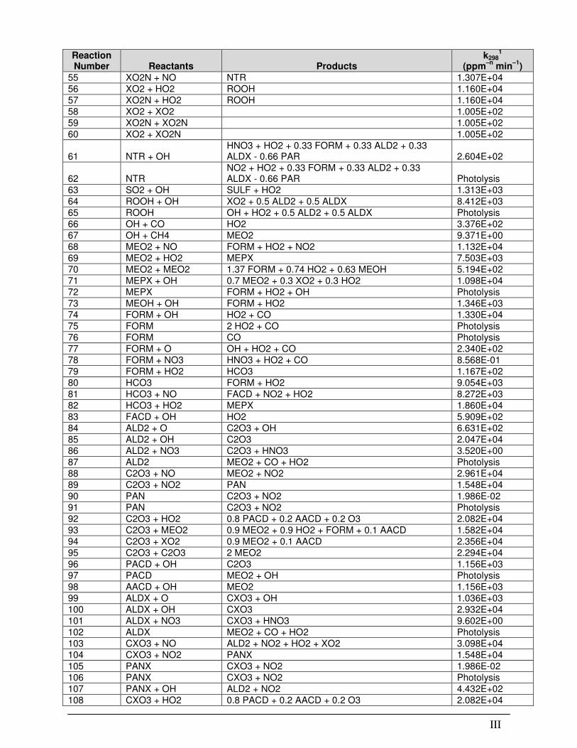
III

Reaction Number

Reactants

Products

k2981

(ppm–n

min–1

)

55 XO2N + NO NTR 1.307E+04

56 XO2 + HO2 ROOH 1.160E+04

57 XO2N + HO2 ROOH 1.160E+04

58 XO2 + XO2 1.005E+02

59 XO2N + XO2N 1.005E+02

60 XO2 + XO2N 1.005E+02

61 NTR + OH HNO3 + HO2 + 0.33 FORM + 0.33 ALD2 + 0.33 ALDX - 0.66 PAR 2.604E+02

62 NTR NO2 + HO2 + 0.33 FORM + 0.33 ALD2 + 0.33 ALDX - 0.66 PAR Photolysis

63 SO2 + OH SULF + HO2 1.313E+03

64 ROOH + OH XO2 + 0.5 ALD2 + 0.5 ALDX 8.412E+03

65 ROOH OH + HO2 + 0.5 ALD2 + 0.5 ALDX Photolysis

66 OH + CO HO2 3.376E+02

67 OH + CH4 MEO2 9.371E+00

68 MEO2 + NO FORM + HO2 + NO2 1.132E+04

69 MEO2 + HO2 MEPX 7.503E+03

70 MEO2 + MEO2 1.37 FORM + 0.74 HO2 + 0.63 MEOH 5.194E+02

71 MEPX + OH 0.7 MEO2 + 0.3 XO2 + 0.3 HO2 1.098E+04

72 MEPX FORM + HO2 + OH Photolysis

73 MEOH + OH FORM + HO2 1.346E+03

74 FORM + OH HO2 + CO 1.330E+04

75 FORM 2 HO2 + CO Photolysis

76 FORM CO Photolysis

77 FORM + O OH + HO2 + CO 2.340E+02

78 FORM + NO3 HNO3 + HO2 + CO 8.568E-01

79 FORM + HO2 HCO3 1.167E+02

80 HCO3 FORM + HO2 9.054E+03

81 HCO3 + NO FACD + NO2 + HO2 8.272E+03

82 HCO3 + HO2 MEPX 1.860E+04

83 FACD + OH HO2 5.909E+02

84 ALD2 + O C2O3 + OH 6.631E+02

85 ALD2 + OH C2O3 2.047E+04

86 ALD2 + NO3 C2O3 + HNO3 3.520E+00

87 ALD2 MEO2 + CO + HO2 Photolysis

88 C2O3 + NO MEO2 + NO2 2.961E+04

89 C2O3 + NO2 PAN 1.548E+04

90 PAN C2O3 + NO2 1.986E-02

91 PAN C2O3 + NO2 Photolysis

92 C2O3 + HO2 0.8 PACD + 0.2 AACD + 0.2 O3 2.082E+04

93 C2O3 + MEO2 0.9 MEO2 + 0.9 HO2 + FORM + 0.1 AACD 1.582E+04

94 C2O3 + XO2 0.9 MEO2 + 0.1 AACD 2.356E+04

95 C2O3 + C2O3 2 MEO2 2.294E+04

96 PACD + OH C2O3 1.156E+03

97 PACD MEO2 + OH Photolysis

98 AACD + OH MEO2 1.156E+03

99 ALDX + O CXO3 + OH 1.036E+03

100 ALDX + OH CXO3 2.932E+04

101 ALDX + NO3 CXO3 + HNO3 9.602E+00

102 ALDX MEO2 + CO + HO2 Photolysis

103 CXO3 + NO ALD2 + NO2 + HO2 + XO2 3.098E+04

104 CXO3 + NO2 PANX 1.548E+04

105 PANX CXO3 + NO2 1.986E-02

106 PANX CXO3 + NO2 Photolysis

107 PANX + OH ALD2 + NO2 4.432E+02

108 CXO3 + HO2 0.8 PACD + 0.2 AACD + 0.2 O3 2.082E+04

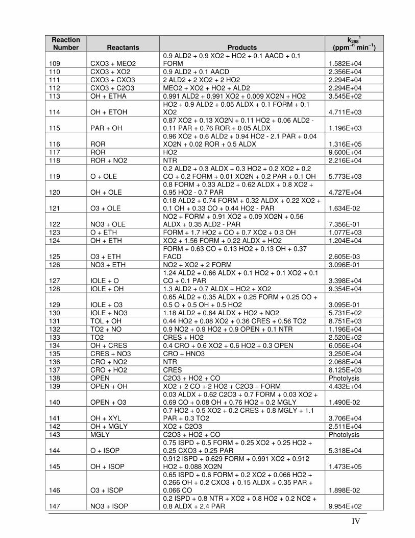
IV

Reaction Number

Reactants

Products

k2981

(ppm–n

min–1

)

109 CXO3 + MEO2 0.9 ALD2 + 0.9 XO2 + HO2 + 0.1 AACD + 0.1 FORM 1.582E+04

110 CXO3 + XO2 0.9 ALD2 + 0.1 AACD 2.356E+04

111 CXO3 + CXO3 2 ALD2 + 2 XO2 + 2 HO2 2.294E+04

112 CXO3 + C2O3 MEO2 + XO2 + HO2 + ALD2 2.294E+04

113 OH + ETHA 0.991 ALD2 + 0.991 XO2 + 0.009 XO2N + HO2 3.545E+02

114 OH + ETOH HO2 + 0.9 ALD2 + 0.05 ALDX + 0.1 FORM + 0.1 XO2 4.711E+03

115 PAR + OH 0.87 XO2 + 0.13 XO2N + 0.11 HO2 + 0.06 ALD2 - 0.11 PAR + 0.76 ROR + 0.05 ALDX 1.196E+03

116 ROR 0.96 XO2 + 0.6 ALD2 + 0.94 HO2 - 2.1 PAR + 0.04 XO2N + 0.02 ROR + 0.5 ALDX 1.316E+05

117 ROR HO2 9.600E+04

118 ROR + NO2 NTR 2.216E+04

119 O + OLE 0.2 ALD2 + 0.3 ALDX + 0.3 HO2 + 0.2 XO2 + 0.2 CO + 0.2 FORM + 0.01 XO2N + 0.2 PAR + 0.1 OH 5.773E+03

120 OH + OLE 0.8 FORM + 0.33 ALD2 + 0.62 ALDX + 0.8 XO2 + 0.95 HO2 - 0.7 PAR 4.727E+04

121 O3 + OLE 0.18 ALD2 + 0.74 FORM + 0.32 ALDX + 0.22 XO2 + 0.1 OH + 0.33 CO + 0.44 HO2 - PAR 1.634E-02

122 NO3 + OLE NO2 + FORM + 0.91 XO2 + 0.09 XO2N + 0.56 ALDX + 0.35 ALD2 - PAR 7.356E-01

123 O + ETH FORM + 1.7 HO2 + CO + 0.7 XO2 + 0.3 OH 1.077E+03

124 OH + ETH XO2 + 1.56 FORM + 0.22 ALDX + HO2 1.204E+04

125 O3 + ETH FORM + 0.63 CO + 0.13 HO2 + 0.13 OH + 0.37 FACD 2.605E-03

126 NO3 + ETH NO2 + XO2 + 2 FORM 3.096E-01

127 IOLE + O 1.24 ALD2 + 0.66 ALDX + 0.1 HO2 + 0.1 XO2 + 0.1 CO + 0.1 PAR 3.398E+04

128 IOLE + OH 1.3 ALD2 + 0.7 ALDX + HO2 + XO2 9.354E+04

129 IOLE + O3 0.65 ALD2 + 0.35 ALDX + 0.25 FORM + 0.25 CO + 0.5 O + 0.5 OH + 0.5 HO2 3.095E-01

130 IOLE + NO3 1.18 ALD2 + 0.64 ALDX + HO2 + NO2 5.731E+02

131 TOL + OH 0.44 HO2 + 0.08 XO2 + 0.36 CRES + 0.56 TO2 8.751E+03

132 TO2 + NO 0.9 NO2 + 0.9 HO2 + 0.9 OPEN + 0.1 NTR 1.196E+04

133 TO2 CRES + HO2 2.520E+02

134 OH + CRES 0.4 CRO + 0.6 XO2 + 0.6 HO2 + 0.3 OPEN 6.056E+04

135 CRES + NO3 CRO + HNO3 3.250E+04

136 CRO + NO2 NTR 2.068E+04

137 CRO + HO2 CRES 8.125E+03

138 OPEN C2O3 + HO2 + CO Photolysis

139 OPEN + OH XO2 + 2 CO + 2 HO2 + C2O3 + FORM 4.432E+04

140 OPEN + O3 0.03 ALDX + 0.62 C2O3 + 0.7 FORM + 0.03 XO2 + 0.69 CO + 0.08 OH + 0.76 HO2 + 0.2 MGLY 1.490E-02

141 OH + XYL 0.7 HO2 + 0.5 XO2 + 0.2 CRES + 0.8 MGLY + 1.1 PAR + 0.3 TO2 3.706E+04

142 OH + MGLY XO2 + C2O3 2.511E+04

143 MGLY C2O3 + HO2 + CO Photolysis

144 O + ISOP 0.75 ISPD + 0.5 FORM + 0.25 XO2 + 0.25 HO2 + 0.25 CXO3 + 0.25 PAR 5.318E+04

145 OH + ISOP 0.912 ISPD + 0.629 FORM + 0.991 XO2 + 0.912 HO2 + 0.088 XO2N 1.473E+05

146 O3 + ISOP

0.65 ISPD + 0.6 FORM + 0.2 XO2 + 0.066 HO2 + 0.266 OH + 0.2 CXO3 + 0.15 ALDX + 0.35 PAR + 0.066 CO 1.898E-02

147 NO3 + ISOP 0.2 ISPD + 0.8 NTR + XO2 + 0.8 HO2 + 0.2 NO2 + 0.8 ALDX + 2.4 PAR 9.954E+02

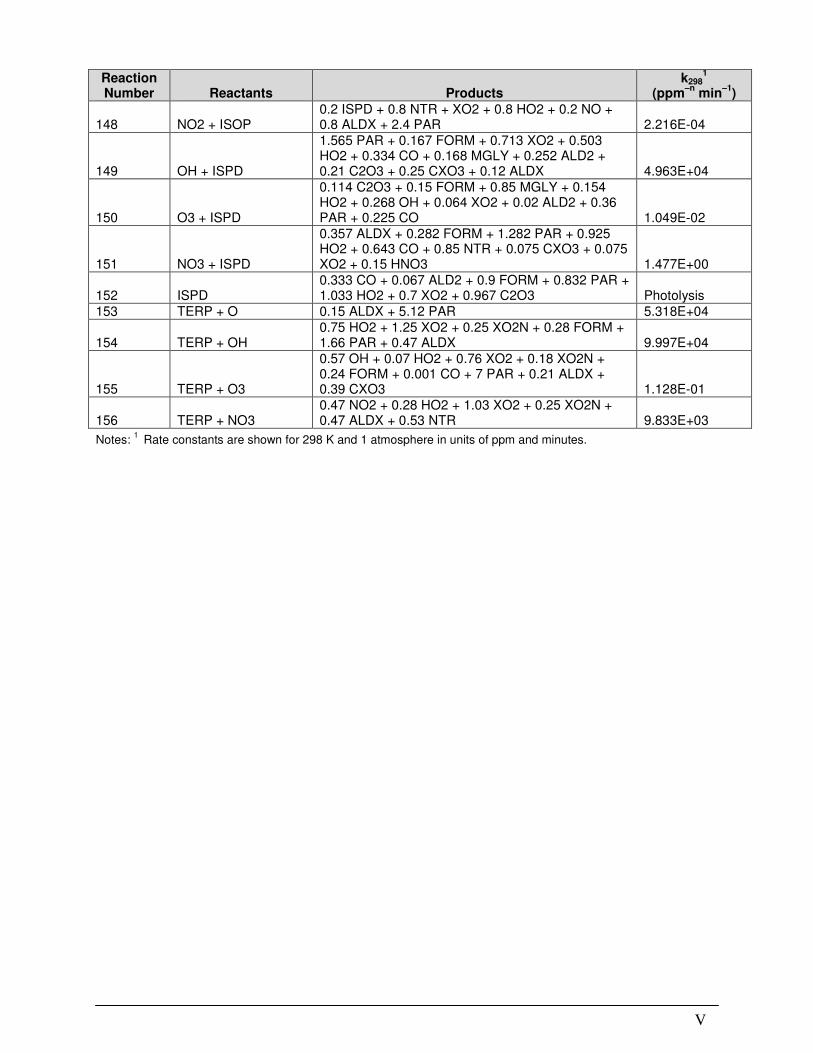
V

Reaction Number

Reactants

Products

k2981

(ppm–n

min–1

)

148 NO2 + ISOP 0.2 ISPD + 0.8 NTR + XO2 + 0.8 HO2 + 0.2 NO + 0.8 ALDX + 2.4 PAR 2.216E-04

149 OH + ISPD

1.565 PAR + 0.167 FORM + 0.713 XO2 + 0.503 HO2 + 0.334 CO + 0.168 MGLY + 0.252 ALD2 + 0.21 C2O3 + 0.25 CXO3 + 0.12 ALDX 4.963E+04

150 O3 + ISPD

0.114 C2O3 + 0.15 FORM + 0.85 MGLY + 0.154 HO2 + 0.268 OH + 0.064 XO2 + 0.02 ALD2 + 0.36 PAR + 0.225 CO 1.049E-02

151 NO3 + ISPD

0.357 ALDX + 0.282 FORM + 1.282 PAR + 0.925 HO2 + 0.643 CO + 0.85 NTR + 0.075 CXO3 + 0.075 XO2 + 0.15 HNO3 1.477E+00

152 ISPD 0.333 CO + 0.067 ALD2 + 0.9 FORM + 0.832 PAR + 1.033 HO2 + 0.7 XO2 + 0.967 C2O3 Photolysis

153 TERP + O 0.15 ALDX + 5.12 PAR 5.318E+04

154 TERP + OH 0.75 HO2 + 1.25 XO2 + 0.25 XO2N + 0.28 FORM + 1.66 PAR + 0.47 ALDX 9.997E+04

155 TERP + O3

0.57 OH + 0.07 HO2 + 0.76 XO2 + 0.18 XO2N + 0.24 FORM + 0.001 CO + 7 PAR + 0.21 ALDX + 0.39 CXO3 1.128E-01

156 TERP + NO3 0.47 NO2 + 0.28 HO2 + 1.03 XO2 + 0.25 XO2N + 0.47 ALDX + 0.53 NTR 9.833E+03

Notes: 1 Rate constants are shown for 298 K and 1 atmosphere in units of ppm and minutes.