Cultural Distance and Housing Prices: Evidence from the ...

Cultural Distance and Housing Prices: Evidence from the Australian Housing Market*

Maggie R. Hu School of Banking and Finance, UNSW Business School, Australia

Tel: 61-2-93855623 Email: [email protected]

Adrian D. Lee

Finance Discipline Group, University of Technology Sydney Tel: 61-2-95147765

Email: [email protected]

Latest draft: August 24, 2015

Abstract:

We investigate whether cultural distance between a buyer’s ethnicity and the neighborhood affects a

home’s selling price. Utilizing individual home sales of culturally diverse Sydney, Australia, we

find a negative relationship between the buyer’s cultural distance to the neighborhood and the

selling price; consistent with buyer preference for similar cultures and inconsistent with cultural

distance being an information friction. Home culture preference is strongest for ethnicities from

recent migration waves, particularly East Asia. Our results are robust to endogeneity and selection

bias. The findings have implications on the role of cultural demographic shifts on housing prices.

Key words: culture distance, housing price, information friction, home culture preference JEL Classification Code: R00, O18, P22, R21

* We thank Doug Foster, Marco Navone, Talis Putnins, Dugald Tinch, participants at the 2015 Asian Global Real Estate Summit and seminar part icipants at the University of Technology Sydney and University of Tasmania for help ful comments and feedback. Lee acknowledges funding for the University of Technology Sydney Business School Research Grant.

1

mailto:[email protected]

mailto:[email protected]

1. Introduction

We analyze to what extent culture affects the housing transaction prices in Sydney,

Australia’s largest and most culturally diverse city. 1 Culture has been alluded to as a priced factor in

hedonic house pricing although never directly tested. For example the introductory chapter of Pace

and LeSage (2009) refers to culture as a latent unobservable influence in hedonic house pricing. We

measure culture’s effect by characterizing the cultural traits inherited at the individual home buyer’s

level using ethnicity as a proxy for culture, which can be treated as largely invariant over an

individual’s life (e.g. Guiso, Sapienza and Zingales (2006)). Specifically, we investigate whether

the cultural distance between the home buyer’s ethnicity and the ethnicity profile of the property’s

neighborhood affects the home's selling price.

Whether and how cultural distance affects housing transaction prices is ambiguous ex-ante.

There are two competing hypotheses we evaluate. On one hand, the information friction hypothesis

posits that home buyers who are more culturally distant from the culture of a property’s

neighborhood are faced with higher search costs and greater information friction to access the local

property market. It would be harder for them to arrive at the efficient price in the housing market,

and therefore they might be forced to pay a higher price for their homes. On the other hand, the

home culture preference hypothesis argues that home buyers prefer locations with greater cultural

similarity, and are willing to pay more for homes in those locations. People in general prefer to live

in a community or neighborhood with similar cultural background (e.g. Saiz (2007)).

Despite culture being a possibly priced factor, the literature is scant on the effect of culture

on housing prices. Recent work suggests that buyers prefer and pay more to live with people of the

same background or ethnicity. For example Li (2014) finds that neighborhoods in Toronto, Canada

with more concentrated minorities have higher housing prices due to buyers valuing social

interactions with own ethnicity higher than with others. Wong (2013) finds preferences for own-

ethnicity are inverted U-shaped in that after a certain amount of own-ethnicity, a neighborhood will

1 For example in the 2011 Australian Bureau of Statistics Census, of the 4,028,524 Sydney urban area respondents, 41.9% were born overseas and 63.8% have at least one parent born overseas.

2

prefer other ethnicities. Culture-related barriers such as language may also act as a friction making

immigrants willing to pay more for housing. For example Fischer (2012) finds that non common

language immigrants to Switzerland are less price-sensitive to house price changes than common

language immigrants. Fischer's finding is consistent with non common language immigrants

valuing local immigrant-specific amenities more due to language acting as a friction for integration.

Employing a transaction level residential property dataset of the Sydney metropolitan area

from 2006 to 2013, we empirically examine the role of culture distance on housing prices. Home

buyer ethnicity is inferred from their surname using a hand collected database of surnames and

ethnicity from various internet sources. We apply the cultural framework of Hofstede (2001) to

measure the cultural distance between the homebuyer’ country of origin and the suburb of the house.

We employ four versions of the suburb’s ethnicity measure using either ancestry or birthplace of the

neighborhood and four or six Hofstede (2001) cultural dimensions . Neighborhood ancestry and

birthplace characteristics are from on the Australian Bureau of Statistics Census snapshots on the

demographics of a neighborhood.

Our main result is that culture distance has a significantly negative impact on housing price.

We show that the greater is the cultural distance between the homebuyer’ country of origin and the

suburb of the house, the lower is the price in that transaction, ceteris paribus. Specifically, if the

cultural distance between a homebuyer with the suburb increases by one point, roughly the

difference between the average Australian and Chinese buyer's cultural distance, housing price

reduces by 1.1% or AUD$7,509 based on the sample mean sales price of AUD$682,650. The

amount is both economically sizeable and statistically significant. This finding suggests that

homebuyers are willingly to pay higher prices for homes in neighborhoods which are closer to their

culture of origin, which provides strong support for the home culture preference hypothesis. Our

regression models control for a long list of housing characteristics, such as area size, property type,

location, type of sale, in additional to buyer ethnicity fixed effect, year and month fixed effects,

3

with robust standard errors clustered at the suburb level. Furthermore the results are robust to

endogeneity and selection bias.

Considering that different ethnicity groups may display varying degrees of home culture

preference, we also explore the extent to which culture distance affects the housing prices for

regions of the world. Some ethnicities may be more recent migrants into Australia, and have strong

emotional and cultural bond with their home country, and therefore may display stronger home

cultural preferences. We extend our baseline analysis by examining ethnicities by region. Our result

show that Asian (East, South-East and South) ethnicities have negative and statistically significant

CD whereas other ethnicities (e.g. African, Australian, Middle Eastern and Europeans (East, North,

South and West) do show not statistically significant CD. The interpretation of the result is that

since people from the European regions came to Australia relatively early compared with Asian

immigrants; their ties to their home country are weaker. Also Australian local culture bears a higher

degree of resemblance with that of the European area.

Our paper contributes to the literature in several ways. First we are able to infer the ethnicity

of the buyer at the sales level and so measure individual buyer's willingness to pay based on their

cultural distance to a neighborhood. As such we have a more direct method of measuring buyer

preferences than inferring flows from changes in the ethnic mix of residents as in Wong (2013) or

using only Census data as in Li (2014). Second we look at preferences of homeowners using

cultural distance rather than own ethnicity shares. This allows us to test whether buyers are sensitive

to other ethnicities based on how culturally close they are. This differs to Wong (2013) who looks at

own ethnicity share though does not consider that some ethnicities are more culturally compatible

than others. Furthermore we are able to instrument cultural distance using genetic distance of

ethnicities and so address endogeneity using two-stage least squares. Being able to address

endogeneity in buyer preferences for housing is a non-trivial issue. For example, Wong (2013)

addresses endogeneity of ethnic preferences by looking at ethnic quotas in Singapore housing

blocks and seeing how constrained blocks are to ethnic quotas.

4

The paper is related to several strands of the literature. Culture plays an important role in

shaping the behavior and decision making of individuals (e.g., Hermalin (2001)). The significance

of cultural distance in investment decisions is highlighted in prior works. Specifically, studies have

shown that cultural distance provides important explanations for the magnitude of the flow of both

debt (Aggarwal, Kearney and Lucey (2012)) and equity (Siegel, Licht and Schwartz (2013))

between countries, loan contract terms (Giannetti and Yafeh (2012)), the extent of investor home

bias (Beugelsdijk and Frijns (2010); Anderson, Fedenia, Hirschey and Skiba (2011)), and the degree

of cross-border merger and acquisitions activity (Ahern, Daminelli and Fracassi (2012)). While

these papers examine the impact of cultural distance on the investment decisions of investors and

corporate managers, we apply it to individual home buyers within a city.

2. Background

2.1 Ethnicity and Immigration in Australia

During the enforcement of the White Australia policy from 1901 to 1958, much of

Australia’s cultural diversity from its Asian neighbors, particularly China and India, was

extinguished. This meant that the predominant ethnicities were white Europeans, particularly

Anglo-Saxons.

After the relaxation of White Australia policy and concurrent to the end of World War II,

there were several waves of migration activities. Appendix 1 provides a guide of when peak

migration occurs from other countries from 1954 to 2011.2 We collect top ten overseas countries of

birth by percentage of the Australian population from the Australian Census from 1954 to 2011.

The table reports for each top ten birthplace, the census year entry into the top ten and the census

year and figure of when the birthplace was at the peak of the total percentage of the Australian

population.

2 Note that population by ethnicity only started being collected from 2006. 5

Anglo-Saxons (mainly Irish and UK) experienced peak population in 1954. In the 1950’s

and 60’s, the peak population occurs for Eastern and Western Europe namely the Dutch, Germans

and Polish. From the 1970’s, the Southern Europeans (Greeks, Italians and Maltese) had population

peaks. In the 1980’s Lebanese migration peaked and in the 1990’s it peaked for Yugoslavia. For

both the Lebanese and Yugoslavs the peaks follow the outbreak of civil war in their respective

countries. In the 2010’s Asian countries, China, India, Malaysia, Philippines and Vietnam

experience their peak population as well as for neighboring Commonwealth countries New

Zealanders and South Africans. Asian countries entered the top ten in the 1990’s suggesting Asians

are the most recent wave of new migrants. In summary, the most established ethnicity in Australia

are the Anglo-Saxons, followed by Western Europeans, Southern Europeans, Middle East, Asia and

New Zealand. The sequencing is important as cultural distance sensitivity may be weaker for more

established ethnicities than recent migrants.

2.2 Culture and Investment Decision

There is a developing literature on the affect of culture on investment decisions. The papers

find consistent that cultural differences along several dimensions between two countries negatively

affects investment between the two, controlling for other factors. For example higher cultural

distance between two countries is related to lower portfolio investment and direct investment (e.g.

Guiso, Sapienza and Zingales (2009)), lower allocation to foreign investments (e.g. Beugelsdijk and

Frijns (2010) and Anderson et al. (2011)), smaller bank loans with higher interest rates (e.g.

Giannetti and Yafeh (2012)) and lower cross-border merger volume (e.g. Ahern et al. (2012)).

Overall, cultural difference between countries appears to act as a friction between countries in a

significant manner affecting the size of investment and value generation between countries.

Our paper while usually a cultural distance variable differs in several aspects to the literature.

First we look at the buying behavior of ethnicities in one large city instead of cross-border

transactions. As such cross-country differences such as in trade or legal frameworks need not factor

6

into our analysis. Second we look at cultural differences between buyer and the population-

weighted ethnic mix in the neighborhood instead of country pairs. Such analysis differs to the usual

cross-country pair analysis of the literature and represents a novel method to apply cultural distance.

Third we investigate the relationship of cultural distance to housing prices at the individual housing

transaction level whereas other studies focus on the country trade level (e.g. Guiso et al. (2006)) or

on public company equity (e.g. Beugelsdijk and Frijns (2010)). As such we investigate the

relationship of cultural distance at a very granular level. While Wong (2013) considers ethnicity

preferences of home buyers to their own ethnicity, we further analyse the preference of home

buyers to other ethnicities using the cultural distance measure.

3. Data

The principal data set we use is individual housing transactions in the Sydney metropolitan

area from 2006 to 2013 from Australian Property Monitors (APM). 3 The dataset includes the sales

price, transaction date, property address, number of bedrooms and bathrooms, whether the parking,

area size of block of land, other housing characteristics (garage, balcony, ocean views, etc.) and

owner and vendor names. Sales prices and area sizes at the 1st and 99th percentile are winsorized to

remove outliers. Hofstede culture dimensions are obtained from its respective websites. 4 Other

datasets used include Australian Bureau of Statistics (ABS) Census snapshots on the demographics

of a suburb (e.g. ancestry, country of birth) in 2006 and 2011. Further, we use genetic distance

between ethnicities from Spolaore and Wacziarg (2009).

Table 1 reports mean summary statistics for our entire sample of 208,8785 sales and across

the top twenty buyer ethnicities by sales. 6 The complete list of ethnicities and regions that we use

are in Appendix 2. The average house price is $682,650 with 59% of sales being houses, an average

3 APM is one of Australia’s leading national supplier of online property price information to the banks, financial markets, professional real estate agents and consumers. See more details at www.apm.com.au 4 http://www.geerthofstede.eu/research--vsm 5 210,269 when including Jewish and South African surnames. 6 The top 20 ethnicities is reported for conciseness.

7

http://www.apm.com.au/

http://www.geerthofstede.eu/research--vsm

size of 3900 square feet, 2.93 bedrooms and 1.61 bathrooms. 86% of homes have parking and 16%

were sold at an auction. Australians (Anglo-Saxon) buyers make up about 35 percent of our sample

consistent with Australians being the majority ethnicity in Sydney. Australians on average paid

$770,490 for a home, higher than the overall sample average though housing characteristics were

similar to the overall sample average. The second largest buyers are Chinese making up about 19%

of the sample, followed by Arabic making up about 10% of the sample. Generally, non-European

ethnicities tend to pay less and buy larger homes than the average buyer which suggests that they

tend to buy in lower priced and less dense suburbs.

4. Methodology

In this section we first describe how we classify owner ethnicity from buyer surnames. We

then show how we calculate cultural distance measures between buyers and neighborhoods. Finally

we describe our regression framework linking housing prices to cultural distance and how we

address issues of endogeneity and selection bias.

4.1 Buyer Ethnicity Classification

In order to calculate cultural distance measures we require the ethnicity of the owner. We

use the owner’s surname to identify the ethnicity of the buyer using a hand collected database of

surnames and ethnicity from various internet sources. Surnames with more than one ethnicity (e.g.

the surname Lee could be Anglo-Saxon, Chinese or Korean) are dropped. The surname database has

been hand collected from free internet sources such as Wikipedia and various surname databases.7

For South African surnames, we use the list in Rosenthal (1965). For names unmatched by our

database, we also a name to ethnicity classifier 8 from Ambekar, Ward, Mohammed, Male and

Skiena (2009) and as Pool, Stoffman and Yonker (2014) use to match Arabic, British (Australian),

French, Indian, Italian or Jewish names when the predicted probability of an ethnicity by the

7 For example: the internet surname database: www.surnamedb.com 8 Available from http://www.textmap.com/ethnicity/

8

http://www.surnamedb.com/

algorithm is above 85 percent. We remove buyers with multiple owners of different ethnicities. We

remove company owners which make up about 2.5% of the sample. Using these filters we are able

to match 54% of sales transaction to an ethnicity.

4.2 Cultural Distance Measures

We calculate the cultural distance based on Hofstede (2001), one of the most widely used

cultural frameworks in empirical work. Hofstede (2001) constructs culture scores on the basis of the

following six dimensions: power distance, uncertainty avoidance, individualism versus collectivism,

masculinity versus femininity, long-term orientation and indulgence versus restraint. The cultural

distance (CD) here is defined as the weighted Euclidean distance between the culture value of the

home buyer's ethnicity and the average person's culture value in the suburb (neighborhood) of the

property. Ethnicity of the suburb is based on the suburb's ancestry or birthplace from ABS Census

2006 and 2011 records. For years between 2006 and 2011 where there is no census information we

impute demographic information. For 2012 and 2013, we assume the demographic information is

the same as for 2011. 𝐶𝐷𝑖,𝑠,𝑡 measures the cultural distance between buyer i’s ethnicity and the

culture of suburb s in year t:

𝐶𝐷𝑖,𝑠,𝑡 = ∑ 𝑤𝑗,𝑠,𝑡 ∗ 𝐶𝐷𝑖,𝑗 ,𝑠,𝑡𝐽𝑗=1 = ∑ 𝑤𝑗,𝑠,𝑡 ∗ �∑ �𝐶𝑖,𝑘 − 𝐶𝑗,𝑘,𝑠�

2/𝑉𝑘𝑁𝑘=1

𝐽𝑗=1 (1)

where

𝑪𝒊,𝒌 is buyer of sale 𝑖’s ethnicity culture value along the k-th culture dimension;

𝑪𝒋,𝒌,𝒔 ethnicity group 𝑗’s value on the k-th culture dimension in suburb s, j=1…J;

𝑽𝒌 is the variance of the culture value of the dimension k;

𝒘𝒋,𝒔,𝒕 is the percentage of ethnicity group 𝑗’s population in suburb s in year t;

There are in total J ethnicity groups and K culture dimensions.

Based on this formula, we can compute a weighted measure of cultural distance of a buyer

to the home’s suburb. The higher the score on the cultural distance measure, the greater the cultural

9

difference between buyer i's culture and the cultural mix of the suburb. For robustness, we also

measure the suburb's ethnicity by birthplace instead of ancestry and use all six dimensions or just

four dimensions excluding long-term orientation and indulgence versus restraint.

Table 2 reports cultural distance statistics for the entire sample and across the top twenty

ethnicities. Over the entire sample, average CD is 1.99. The statistic may be interpreted as the mean

buyer's suburb is 1.99 standard deviations away from the buyer's ethnicity cultural dimension score.

Australian buyers have the lowest average CD of 1.34 across all ethnicities consistent with most

suburbs having a majority Anglo-Saxon demographic. Note that the overall minimum cultural

distance is 0.59 for Australians which suggests that all suburbs have a diverse mix of ethnic

backgrounds. Arabics, Australians, Chinese and Vietnamese have the highest CD standard deviation

consistent with both groups buying into suburbs with a broad range of cultural distance to

themselves. Other ethnicity groups have lower standard deviations and ranges (max minus min CD)

suggesting that they tend to concentrate buys in fewer suburbs. The wide variability in cultural

distance across buyers allows us to test the relationship between buyer prices and cultural distance

to the suburb.

4.3 Regression Framework

After measuring cultural distance we then estimate a hedonic housing price models based on

the following empirical specification and variable definitions:

ln(𝑃𝑖𝑠𝑡) = 𝛼𝑡 + 𝛽𝑘𝐶𝐷𝑖𝑠𝑡 + 𝑝𝑟𝑜𝑝𝑒𝑟𝑡𝑦 𝑐ℎ𝑎𝑟+ 𝜇𝑠 + δ𝑖+𝛾𝑡 + τ𝑡 + 𝜀𝑖𝑡 (2)

Where

𝒍𝒏 (𝑷𝒊𝒔𝒕) denotes logarithm of house prices paid by buyer of sale i at suburb s at time t;

𝒑𝒓𝒐𝒑𝒆𝒓𝒕𝒚 𝒄𝒉𝒂𝒓 are various property characteristics such as number of bedrooms, number of

bathrooms, parking, property type and area size9;

𝝁𝒔 is the suburb location specific fixed effect;

9 Appendix 3 shows the full list of housing characteristics that we use. 10

δ i is buyer’s ethnicity fixed effects.

𝜸𝒕 is year/quarter fixed effect;

τ t is a monthly time trend;

A positive and statistically significant 𝛽𝑘 suggests that buyers tend to pay higher prices with

greater cultural distance to the suburb consistent with the information friction hypothesis. On the

other hand if we find a negative and statistically significant 𝛽𝑘 this suggests evidence consistent to

the home culture preference hypothesis.

There are two inherent problems with the baseline specification estimate using ordinary least

squares: selection bias and endogeneity. First there is selection bias where buyers may self-select

into suburbs based on cultural distance and therefore the sampling is non-random. For example if

buyers tend to purchase in suburbs with a low cultural distance to themselves then we would not

observe buyers in high cultural distance which would bias our results. As such our strategy is to use

a Heckman two stage selection model. In the first stage we run the following probit model across

ethnicities at the suburb/quarter level:

Pr (𝐵𝑢𝑦𝑗𝑠𝑡 = 1|𝑋) = 𝐹(𝛼0 + 𝛽1𝐶𝐷𝑗𝑠𝑡 + 𝛽2𝑙𝑎𝑔𝑦𝑏𝑢𝑦𝑗𝑠𝑡 + 𝜇𝑠 + δ𝑗+𝛾𝑡 + 𝜀𝑗𝑠𝑡 ) (3)

with the dependent variable being a dummy of 1 if a given ethnicity buys in a suburb in a

given quarter and 0 otherwise. Our instrumental variable is lagybuyjst , a dummy of 1 if there is any

sale by the buyer’s ethnicity in the prior twelve months in suburb s and 0 otherwise. We obtain the

inverse mills ratio from the probit estimate and use it as an additional independent variable in

equation 2. The instrumental variable is motivated by the literature on peer group effects. It has

been found that peer group effects such as within ethnicity groups strongly influences the behavior

and decisions of an individual, controlling for other factors. See for example in car purchases

(Grinblatt, Keloharju and Ikäheimo (2008) , employment outcomes (Bayer, Ross and Topa (2008),

Patacchini and Zenou (2012)) welfare participation (Bertrand, Luttmer and Mullainathan (2000),

Betrand, Luttmer and Mullainathan (2000)) and worker productivity (Mas and Moretti (2009)).

Importantly as a valid instrument, this peer effect influences the decision and not the price paid by 11

the individual. Consistent with this effect, Hvide and Östberg) find stock market decisions of

individuals are positively correlated with those of co-workers and this positive correlation is not

associated with positive future returns. As such we hypothesize that prior buying by the same

ethnicity is a valid instrument as it increases the probability of buying by the ethnicity group

however has no effect on the price paid.

Endogeneity is also present in our baseline specification as there may be an omitted

variable bias where unobserved characteristics of the buyer, home or neighborhood may be

correlated with both prices and cultural distance. To address endogeneity we identify cultural

distance with genetic distance following Guiso et al. (2009) and Ahern et al. (2012). As Ahern et al.

(2012) describes, genetic distance is 'a measure of the probability that two random alleles (DNA

variations) from two populations will be different, based on the dominant population of a country'.

Genetic distance is correlated to cultural distance as ethnicities that share common ancestors will

tend to inherit both biological and cultural similarities (e.g. Spolaore and Wacziarg (2009)).

However as genetic similarities take many generations to eventuate in ethnicity, it is unrelated to

house prices. The first stage regression regresses the buyer's cultural distance on all control

variables including genetic distance as such:

𝐶𝐷𝑖𝑠𝑡 = 𝛼𝑡 + 𝛽𝑘𝐺𝐷𝑖𝑠𝑡 + 𝑝𝑟𝑜𝑝𝑒𝑟𝑡𝑦 𝑐ℎ𝑎𝑟+ 𝜇𝑠 + δ𝑖+𝛾𝑡 + τ𝑡 + 𝜀𝑖𝑡 (4)

where GDist is the genetic distance of buyer i to the population weighted ethnicities in suburb s. We

then use the estimated cultural distance 𝐶𝐷𝚤𝑠𝑡� from the first stage regression in the second stage

instead of 𝐶𝐷𝑖𝑠𝑡 .

To take account for both self-selection and endogeneity we follow the procedure in section

19.6.2 of Wooldridge (2010). The involves the same two-stage instrumental variable and also

including the inverse Mills ratio obtained from running the probit in equation 3 but using 𝐺𝐷𝑖𝑠𝑡

instead of 𝐶𝐷𝑖𝑠𝑡 . We thus report coefficients estimates using OLS, Heckman 2-stage, 2-stage

instrumental variables and a combination of Heckman 2-stage and 2-stage instrumental variable

regression.

12

5. Results

5.1 First Stage Probit

Table 3 reports coefficient estimates of our probit model. Across all measures of cultural

distance the coefficient is negative and statistically significant which suggests that the larger the

cultural distance the lower the probability of an ethnicity group buying into a given suburb. The

finding is consistent with buyer’s having a preference for similar cultures and also Ahern et al.

(2012)'s first stage probit results where higher cultural distance between two countries reduces the

probability of a merger occuring.

Consistent with a peer effect in home buying, lagybuyjst is positive and statistically

significant across all measures of cultural distance which suggests that prior buying in a suburb by

an ethnicity increases the chances of the ethnicity buying in the current quarter. As such it appears

that our instrument is valid.

5.2 Baseline Regression

Table 4 reports coefficient estimates of cultural distance using various regression methods.

Each panel represents the use of a different cultural difference measure. We find the coefficient for

cultural distance is negative and statistically significant across cultural distance measures. It is also

robust when accounting for endogeneity or selection bias, or both together. The exceptions are for

the combined Heckman selection and 2-stage least squares method for cultural distance using

birthplace (the last column of Table 4 Panel B and last column of Table 4 Panel D) although the

coefficient is negative. This is because standard errors of the CD coefficient tend to be much higher

when we apply both Heckman selection and 2-stage least squares.

Generally across CD measures, the coefficient estimates become more negative when

adjusting for self-selection or omitted variable bias suggesting that the ordinary least squares

estimates are biased downwards. The inverse mills ratio across Heckman specifications is

statistically significant that suggesting selection bias is not an issue. 13

The coefficient estimate across measures and methods ranges from -0.009 (Table 4 Panel B,

ordinary least squares) to -0.032 (Table 4 Panel C, two stage least squares). This suggests that a one

standard deviation increase in the cultural distance of a buyer with the suburb reduces the buyer's

price by between 0.9% to 3.2%. For example for ordinary least squares in Table 4 Panel A, a one

standard deviation move in cultural distance reduces housing prices by 1.1% or AUD$7,509 given

the mean sales price of AUD$682,650. As a buyer's cultural distance may range from 0.96 to 4.37,

this is an economically significant amount. Our results therefore support the effect of home culture

preference of buyers.

5.3 Cultural Distance and Ethnicity Interaction

Extending on the baseline results, this section investigates whether the cultural distance

coefficient is heterogeneous amongst ethnicities, particularly that the effect is strongest for more

recent migrants. There is evidence to believe this is the case such as Fischer (2012) finding

immigrant inflows from countries with non-common language country into an area increase housing

prices due to valuing immigrant specific amenities and networks. On the other hand, ethnicities that

have been in Australia for many generations may not have such a strong home culture preference as

they may have a wider amount of amenities to enjoy and their networks may not geographically

concentrated.

We extend our baseline regression by interacting cultural distance to a dummy of one if the

ethnicity of the buyer is from a region as outlined in Appendix 2 (e.g. East Asia), or otherwise. We

interact with regions rather than each ethnicity for conciseness. The groupings also provide a rough

guide of immigration arrival. For example, the earliest mass migration were by Anglo-Saxons

followed by Western and Northern Europeans. The most recent mass migrations were from Asia.

Table 5 reports results for CD and buyer region interaction coefficient estimates. Similar to

our baseline reports we report for each panel the different cultural distance measures and each panel

reports the various regression models.

14

Consistent with more recent migrants being more sensitive to home cultural preference, we

find negative and statistically significant coefficients for cultural distance across all CD measures

and regression methods for East Asia. The coefficient estimates tend also to be much larger than for

CD on the overall sample ranging from -0.014 to -0.050 suggesting that East Asian have a much

more negative CD than the average population. South East Asians also show negative and

statistically significant CD across CD measures although the results are statistically significant

when apply Heckman selection and 2-stage least squares together.

Middle East, South Asia and Southern Europe also show negative and statistically cultural

distance measures although the result is not robust particularly to controlling for endogeneity using

2-stage least squares.

Australians, Eastern Europeans, Northern Europeans and Western Europeans show negative

and statistically insignificant or weakly significant CD coefficients which suggests that these groups

are less affected by cultural distance, consistent with earlier migrants not being sensitive cultural

distance.

Taken together our results provide some evidence that home culture preference appears

related to the recency of migration of the buyer's ethnicity, with the earliest migrants showing no

evidence of home cultural bias.

6. Conclusion

This paper shows that culture distance matters in people’s housing decisions. We develop

two competing hypotheses, i.e., the home culture preference hypothesis and the information friction

hypothesis. Our empirical evidence demonstrates that homebuyers pay higher prices for houses in

suburbs that are closer in culture to their countries of origin, which provides strong support for the

home culture preference hypothesis. For example a one standard deviation increase of cultural

distance between a homebuyer with the suburb causes a 1.1% decrease in home price. The effect of

15

culture distance is economically meaningful, given the sample mean sales price of AUD$682,650.

The results are robust to different cultural distance measures, endogeneity and selection bias.

To show that different ethnicity groups display varying degree of home, we perform a

battery of subsample analysis for the top ten ethnicity group in our sample. Our findings

demonstrate that immigrants particularly from Asia display a greater degree of home culture

preference, whereas we find no or weak statistical significance for buyers from Australia or Europe.

Taken together, our paper provides important insights in the area of culture, foreign

immigrant homebuyers, and housing price. It contributes to the literature on the role of culture

distance in housing market decision making by highlighting the importance of culture aspects in the

residential housing market.

16

References

Aggarwal, R., C. Kearney, and B. Lucey, 2012, Gravity and culture in foreign portfolio investment, Journal of Banking & Finance 36, 525-538.

Ahern, K. R., D. Daminelli, and C. Fracassi, 2012, Lost in translation? The effect of cultural values on mergers around the world, Journal of Financial Economics.

Ambekar, A., C. Ward, J. Mohammed, S. Male, and S. Skiena, 2009, Name-ethnicity classification from open sources, Proceedings of the 15th ACM SIGKDD international conference on Knowledge discovery and data mining (ACM, Paris, France).

Anderson, C. W., M. Fedenia, M. Hirschey, and H. Skiba, 2011, Cultural influences on home bias and international diversification by institutional investors, Journal of Banking & Finance 35, 916-934.

Bayer, P., S. L. Ross, and G. Topa, 2008, Place of Work and Place of Residence: Informal Hiring Networks and Labor Market Outcomes, Journal of Political Economy 116, 1150-1196.

Bertrand, M., E. F. P. Luttmer, and S. Mullainathan, 2000, Network Effects and Welfare Cultures, The Quarterly Journal of Economics 115, 1019-1055.

Beugelsdijk, S., and B. Frijns, 2010, A cultural explanation of the foreign bias in international asset allocation, Journal of Banking & Finance 34, 2121-2131.

Fischer, A. M., 2012, Immigrant language barriers and house prices, Regional Science and Urban Economics 42, 389-395.

Giannetti, M., and Y. Yafeh, 2012, Do cultural differences between contracting parties matter? Evidence from syndicated bank loans, Management Science 58, 365-383.

Grinblatt, M., M. Keloharju, and S. Ikäheimo, 2008, Social Influence and Consumption: Evidence from the Automobile Purchases of Neighbors, Review of Economics and Statistics 90, 735-753.

Guiso, L., P. Sapienza, and L. Zingales, 2006, Does Culture Affect Economic Outcomes?, The Journal of Economic Perspectives 20, 23-48.

Guiso, L., P. Sapienza, and L. Zingales, 2009, Cultural Biases in Economic Exchange?, Quarterly Journal of Economics 124, 1095-1131.

Hermalin, B. E., 2001. Economics and Corporate Culture (John Wiley & Sons Chichester, England). Hofstede, G. H., 2001. Culture's consequences: Comparing values, behaviors, institutions and organizations

across nations (Sage). Hvide, H. K., and P. Östberg, Social interaction at work, Journal of Financial Economics. Li, Q., 2014, Ethnic diversity and neighborhood house prices, Regional Science and Urban Economics 48,

21-38. Mas, A., and E. Moretti, 2009, Peers at Work, American Economic Review 99, 112-45. Pace, R. K., and J. LeSage, 2009, Introduction to spatial econometrics, Boca Raton, FL: Chapman

&Hall/CRC. Patacchini, E., and Y. Zenou, 2012, Ethnic networks and employment outcomes, Regional Science and

Urban Economics 42, 938-949. Pool, V. K., N. Stoffman, and S. E. Yonker, 2014, The people in your neighborhood: Social interactions and

mutual fund portfolios, Journal of Finance forthcoming. Rosenthal, E., 1965. South African Surnames (H. Timmins). Saiz, A., 2007, Immigration and housing rents in American cities, Journal of Urban Economics 61, 345-371. Siegel, J. I., A. N. Licht, and S. H. Schwartz, 2013, Egalitarianism, cultural distance, and foreign direct

investment: A new approach, Organization Science 24, 1174-1194. Spolaore, E., and R. Wacziarg, 2009, The Diffusion of Development, Quarterly Journal of Economics 124,

469-592. Wong, M., 2013, Estimating ethnic preferences using ethnic housing quotas in Singapore, Review of

Economic Studies 80, 1178-1214. Wooldridge, J. M., 2010. Econometric Analysis of Cross Section and Panel Data (Cambridge: MIT Press).

17

Appendix 1 Top Ten Overseas Country of Birth in Australia from 1954 to 2011

We collect top ten overseas country of birth by percentage of the Australian population from the Australian Census from 1954 (just prior to the relaxat ion of the White Australia policy in 1958) to 2011. The table reports for each top ten birthplace, the census year entry into the top ten and the census year and figure of when the birthplace was at the peak of the total percentage of the Australian population. The census year entry and peak provides a guide of the most recent immigration way from the birthplace country.

Census Year Year of Entry Birthplace % of Total Population

1954 1954 Ireland 0.50 1954 1954 UK 6.86 1954 1954 Poland 0.63 1961 1954 Germany 1.04 1961 1954 Netherlands 0.97 1971 1954 Greece 1.26 1971 1954 Italy 2.27 1971 1954 Malta 0.42 1981 1981 Lebanon 0.28 1991 1954 Yugoslavia 0.96 2011 1991 Chinaa 1.48 2011 2001 India 1.37 2011 2011 Malaysia 0.54 2011 1991 Philippines 0.80 2011 1991 Vietnam 0.86 2011 1954 New Zealand 2.25 2011 2006 South Africa 0.68

a excludes Taiwan and Special Administrative Regions

18

Appendix 2 Region and Ethnicities

The table reports the region and ethnicities that the study uses. The ethnicities match with those used in the Hofstede cultural dimensions. Sydney Population statistics are from the 2006 and 2011 Australian Bureau of Statistics Censuses. Ethnicities marked with an astericks only have four cultural dimensions measured.

Region Ethnicity % of Pop. in 2006 Census % of Pop. in 2011 Census Africa Moroccan 0.01 0.01

South African* 0.41 0.43

Australia Australian/British 45.16 42.97 East Asia Chinese 7.84 8.99 Japanese 0.29 0.30 Korean 1.04 1.26 Taiwanese 0.05 0.05 South Asia Bangladeshi 0.28 0.44

Indian 2.20 3.10

Nepalese 0.09 0.41

Sri Lankan 0.46 0.51

South East Asia Indonesian 0.25 0.31 Filipino 1.19 1.38 Malaysian 0.08 0.09 Singaporean 0.02 0.02 Thai 0.23 0.33 Vietnamese 1.65 1.90 Middle East Arabic 3.52 3.72

Israeli/Jewish* 0.08 0.19

Turkish 0.49 0.51

Eastern Europe Croatian 0.71 0.68 Czech 0.11 0.11 Hungarian 0.31 0.28 Polish 0.58 0.53 Romanian 0.08 0.08 Russian 0.39 0.40 Serbian 0.63 0.52 Slovak Republic 0.05 0.06 Northern Europe Danish 0.07 0.07 Estonian 0.03 0.03 Finnish 0.05 0.05 Latvian 0.06 0.05 Lithuanian 0.05 0.05 Norwegian 0.03 0.03 Swedish 0.06 0.06 Southern Europe Greek 2.57 2.43 Italian 3.95 3.82 Maltese 0.75 0.71 Portuguese 0.33 0.33 Western Europe French 0.26 0.28 Dutch 0.49 0.47 German 1.41 1.37 Irish 4.47 4.56 Swiss 0.07 0.07 Total 82.85 83.96

19

Appendix 3 List of Housing Characteristic Variables

Variable Description Beds Number of beds Baths Number of bathrooms Multiple Parking 1 if home has two or more parking spots, 0 otherwise Street type dummies 1 if a certain street type (e.g. avenue, highway, lane, street, road, etc.), 0 otherwise Housing type dummies 1 if a certain housing type (e.g. apartment (condomin ium), house, semi, studio,

townhouse, villa, etc.), 0 otherwise Housing type dummy* Area size

Housing type dummy interacted with land area size of home (square metres).

HasAirConditioning 1 if home has air conditioning, 0 otherwise HasAlarm 1 if home has alarm system, 0 otherwise HasBalcony 1 if home has balcony, 0 otherwise HasBarbeque 1 if home has barbeque, 0 otherwise HasBeenRenovated 1 if home has been renovated, 0 otherwise HasBilliardRoom 1 if home has billiard room, 0 otherwise HasCourtyard 1 if home has courtyard, 0 otherwise HasEnsuite 1 if home has ensuite, 0 otherwise HasFamilyRoom 1 if home has family room, 0 otherwise HasFireplace 1 if home has fire place, 0 otherwise HasGarage 1 if home has garage, 0 otherwise HasHeating 1 if home has heating, 0 otherwise HasInternalLaundry 1 if home has internal laundry, 0 otherwise HasLockUpGarage 1 if home has lock up garage, 0 otherwise HasPolishedTimberFloor 1 if home has polished timber floors, 0 otherwise HasPool 1 if home has swimming pool, 0 otherwise HasRumpusRoom 1 if home has rumpus room, 0 otherwise HasSauna 1 if home has sauna, 0 otherwise HasSeparateDining 1 if home has separate dining room, 0 otherwise HasSpa 1 if home has spa, 0 otherwise HasStudy 1 if home has study room, 0 otherwise HasSunroom 1 if home has sunroom, 0 otherwise HasTennisCourt 1 if home has tennis court, 0 otherwise HasWalkInWardrobe 1 if home has walk in wardrobe, 0 otherwise View dummies 1 if home has a certain view (e.g. bush, city, district, harbour, ocean, park, river, etc.),

0 otherwise

20

Table 1 Summary Statistics of Home Sales

The table reports mean summary statistics for home sales in the Sydney metropolitan area from 2006 to 2013 for the entire sample and for the top 20 buyer ethnicity groups. The data is from Australian Property Monitors. Buyer ethnicity is classified by surname of the buyer. Price is in thousands of Australian dollars. House is a dummy variable equal to one for a house and zero otherwise (e.g. apartment (condominium), house, semi, studio, townhouse, villa , etc), . House area size is in 1,000 square feet. Bed is the number of bedrooms and bath is the number of bathrooms. Parking is a dummy variable equal to one if the home has parking. Auction is a dummy variable equal to one if the home was sold at auction.

Ethnicity Price ($'000) House

House Area Size (1,000

sq ft) Bed Bath Parking Auction N

Australian 770.49 0.59 3.95 2.91 1.62 0.83 0.16 73,114

Chinese 674.48 0.47 3.20 2.89 1.70 0.89 0.15 39,223

Arabic 546.04 0.72 4.84 3.05 1.51 0.88 0.19 20,145

Indian 551.03 0.59 3.92 2.95 1.59 0.89 0.13 17,945

Irish 765.70 0.58 3.78 2.88 1.60 0.83 0.17 14,476

Italian 673.05 0.64 4.17 2.94 1.58 0.87 0.18 12,056

Vietnamese 486.87 0.71 4.50 3.05 1.48 0.86 0.15 8,130

Greek 725.00 0.65 4.01 2.93 1.55 0.85 0.24 5,220

German 790.29 0.57 3.80 2.90 1.64 0.82 0.18 2,656

French 705.10 0.61 4.03 2.92 1.61 0.83 0.17 2,155

Korean 661.89 0.56 4.07 3.00 1.73 0.91 0.15 1,807

Spanish 522.70 0.55 3.44 2.86 1.52 0.86 0.11 1,767

Slovakian 547.66 0.58 3.67 2.89 1.51 0.88 0.14 1,405

Portuguese 577.93 0.56 3.43 2.83 1.54 0.88 0.13 1,352

Polish 638.39 0.52 3.47 2.80 1.54 0.85 0.14 1,171

Maltese 548.95 0.70 5.01 3.04 1.52 0.88 0.11 832

Indonesian 594.11 0.49 2.93 2.77 1.64 0.88 0.13 831

Dutch 777.57 0.56 3.86 2.86 1.63 0.84 0.13 669

Sri Lanka 602.14 0.63 4.45 2.97 1.60 0.89 0.12 539

Japanese 678.74 0.50 3.17 2.62 1.53 0.84 0.11 537

All 682.65 0.59 3.90 2.93 1.61 0.86 0.16 208,878

21

Table 2 Summary Statistics of Cultural Distance between Buyer and Home's Suburb

The table reports summary statistics for the cultural d istance of the buyer to the home's suburb across sales in the Sydney metropolitan area from 2006 to 2013 fo r the entire sample and the top twenty buyer ethnicity groups. Buyer ethnicity is classified by surname of the buyer. Suburb demographic informat ion is from the Australian Bureau of Statistics Census in 2006 and 2011. Cultural distance is measured as the Euclidean distance between the Hofstede cultural d imensions of the buyer's ethnicity to the population weighted ethnicity cultural d imensions in the home's suburb. The cultural dimensions are power distance, uncertainty avoidance, individualis m versus collectivis m, masculinity versus femininity, long-term orientation and indulgence versus restraint.

Ethnicity Mean Std Dev Q1 Median Q3 Min Max N

Australian 1.34 0.47 1.00 1.25 1.56 0.59 3.30 73,114

Chinese 2.49 0.55 2.09 2.51 2.94 1.19 3.60 39,223

Arabic 2.28 0.48 1.93 2.28 2.68 1.35 3.25 20,145

Indian 2.14 0.33 1.95 2.18 2.40 0.81 2.71 17,945

Irish 1.62 0.40 1.31 1.52 1.80 0.87 3.03 14,476

Italian 2.03 0.25 1.87 1.98 2.15 1.17 3.14 12,056

Vietnamese 2.42 0.54 2.09 2.41 2.84 1.35 3.57 8,130

Greek 2.91 0.37 2.63 2.95 3.22 1.91 3.61 5,220

German 1.79 0.27 1.59 1.70 1.91 1.42 3.00 2,656

French 2.70 0.14 2.64 2.74 2.81 2.24 3.17 2,155

Korean 3.05 0.39 2.73 3.08 3.36 2.27 3.86 1,807

Spanish 2.60 0.20 2.45 2.65 2.76 2.05 2.94 1,767

Slovakian 3.67 0.18 3.54 3.68 3.82 3.16 4.10 1,405

Portuguese 3.46 0.37 3.19 3.49 3.76 2.59 4.17 1,352

Polish 2.73 0.17 2.63 2.77 2.86 2.20 3.12 1,171

Maltese 2.75 0.16 2.70 2.79 2.87 2.20 3.12 832

Indonesian 2.76 0.47 2.45 2.77 3.14 1.64 3.80 831

Dutch 3.08 0.19 2.94 3.04 3.18 2.80 3.74 669

Sri Lanka 2.76 0.38 2.52 2.83 3.06 1.81 3.42 539

Japanese 3.29 0.10 3.26 3.32 3.35 2.88 3.72 537

All 1.99 0.73 1.37 1.98 2.53 0.59 4.37 208,878

22

Table 3 First Stage Probit Regression

The table reports coefficient estimates of the probit model in equation 3. The data is home sales from 2006 to 2013 for the Sydney metropolitan area from 2006 to 2013. Buyer ethnicity is classified by surname of the buyer. Cultural distance is measured as the euclidean distance between the Hofstede cultural dimensions of the buyer's ethnicity to the population weighted ethnicity cultural d imensions in the home's suburb. The cultural d imensions are power distance, uncertainty avoidance, individualis m versus collectivis m, masculin ity versus femin inity, long-term orientation and indulgence versus restraint. The ancestry measures use the ancestry of the suburb while the birthplace measures use the birthplace of the suburb to create cultural d istance of buyer to suburb's demographics. Cultural distance measured using 4 d imensions excludes long-term orientation and indulgence versus restraint. p-values are in square brackets. ***, **, * signifies statistical significance at the 1, 5 and 10 percent level.

CD (Ancestry 6 Dimensions)

CD (Birthplace 6 Dimensions)

CD (Ancestry 4 Dimensions)

CD (Birthplace 4 Dimensions)

Intercept 2.677*** 1.536*** 2.114*** 1.444*** [<0.001] [<0.001] [<0.001] [<0.001] CD -0.845*** -0.832*** -0.832*** -0.912*** [<0.001] [<0.001] [<0.001] [<0.001] lagybuy 0.278*** 0.342*** 0.300*** 0.351*** [<0.001] [<0.001] [<0.001] [<0.001] Buyer Ethnicity Fixed Effects Yes Yes Yes Yes Year/Quarter Fixed Effects Yes Yes Yes Yes Cox-Snell R-square 0.2777 0.2737 0.2699 0.2667 Number of Observations 771,420 771,420 807,300 807,300

23

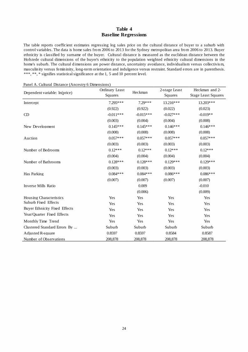
Table 4 Baseline Regressions

The table reports coefficient estimates regressing log sales price on the cultural distance of buyer to a suburb with control variables. The data is home sales from 2006 to 2013 for the Sydney metropolitan area from 2006 to 2013. Buyer ethnicity is classified by surname of the buyer. Cultural distance is measured as the euclidean distance between the Hofstede cultural dimensions of the buyer's ethnicity to the population weighted ethnicity cultural dimensions in the home's suburb. The cultural d imensions are power distance, uncertainty avoidance, individualism versus collectivis m, masculin ity versus femin inity, long-term orientation and indulgence versus restraint. Standard errors are in parenthesis. ***, **, * signifies statistical significance at the 1, 5 and 10 percent level. Panel A. Cultural Distance (Ancestry 6 Dimensions)

Dependent variable: ln(price) Ordinary Least

Squares Heckman 2-stage Least

Squares Heckman and 2-

Stage Least Squares

Intercept 7.295*** 7.29*** 13.216*** 13.203*** (0.922) (0.922) (0.022) (0.023)

CD -0.011*** -0.015*** -0.027*** -0.019** (0.003) (0.004) (0.004) (0.008)

New Development 0.145*** 0.145*** 0.146*** 0.146*** (0.008) (0.008) (0.008) (0.008) Auction 0.057*** 0.057*** 0.057*** 0.057*** (0.003) (0.003) (0.003) (0.003) Number of Bedrooms 0.12*** 0.12*** 0.12*** 0.12*** (0.004) (0.004) (0.004) (0.004) Number of Bathrooms 0.128*** 0.128*** 0.129*** 0.129*** (0.003) (0.003) (0.003) (0.003) Has Parking 0.084*** 0.084*** 0.086*** 0.086*** (0.007) (0.007) (0.007) (0.007) Inverse Mills Ratio 0.009 -0.010 (0.006) (0.009) Housing Characteristics Yes Yes Yes Yes Suburb Fixed Effects Yes Yes Yes Yes Buyer Ethnicity Fixed Effects Yes Yes Yes Yes Year/Quarter Fixed Effects Yes Yes Yes Yes Monthly Time Trend Yes Yes Yes Yes Clustered Standard Errors By ... Suburb Suburb Suburb Suburb Adjusted R-square 0.8597 0.8597 0.8584 0.8587 Number of Observations 208,878 208,878 208,878 208,878

24

Panel B. Cultural Distance (Birthplace 6 Dimensions)




Stage Least Squares Intercept 7.273*** 7.265*** 13.315*** 13.179***

(0.922) (0.922) (0.016) (0.022) CD -0.009* -0.012** -0.014*** -0.010

(0.005) (0.005) (0.003) (0.007) New Development 0.145*** 0.145*** 0.145*** 0.146*** (0.008) (0.008) (0.008) (0.008) Auction 0.057*** 0.057*** 0.057*** 0.057*** (0.003) (0.003) (0.003) (0.003) Number of Bedrooms 0.12*** 0.12*** 0.12*** 0.12*** (0.004) (0.004) (0.004) (0.004) Number of Bathrooms 0.128*** 0.128*** 0.129*** 0.129*** (0.003) (0.003) (0.003) (0.003) Has Parking 0.084*** 0.084*** 0.086*** 0.086*** (0.007) (0.007) (0.007) (0.007) Inverse Mills Ratio 0.008 -0.010 (0.006) (0.012) Housing Characteristics Yes Yes Yes Yes Suburb Fixed Effects Yes Yes Yes Yes Buyer Ethnicity Fixed Effects Yes Yes Yes Yes Year/Quarter Fixed Effects Yes Yes Yes Yes

Monthly Time Trend Yes Yes Yes Yes Clustered Standard Errors By ... Suburb Suburb Suburb Suburb Adjusted R-square 0.8597 0.8597 0.8584 0.8587 Number of Observations 208,878 208,878 208,878 208,878

25

Panel C. Cultural Distance (Ancestry 4 Dimensions)





(0.924) (0.924) (0.022) (0.022) CD -0.014*** -0.017*** -0.032*** -0.021**



26

Panel D. Cultural Distance (Birthplace 4 Dimensions)





(0.925) (0.925) (0.016) (0.022) CD -0.013** -0.015** -0.02*** -0.013



27

Table 5 Cultural Distance and Ethnicity Region Interaction

The table reports coefficient estimates regression log sales price with cultural distance interacted with buyer's ethnicity region to suburb with control variables. The data is home sales from 2006 to 2013 for the Sydney metropolitan area from 2006 to 2013. Buyer ethnicity is classified by surname of the buyer. Cultural d istance is measured as the euclidean distance between the Hofstede cultural d imensions of the buyer's ethnicity to the population weighted ethnicity cultural dimensions in the home's suburb. The cultural dimensions are power distance, uncertainty avoidance, individualis m versus collectivism, masculinity versus femin inity, long-term orientation and indulgence versus restraint. Standard errors are in parenthesis. ***, **, * signifies statistical significance at the 1, 5 and 10 percent level.

Panel A. Cultural Distance (Ancestry 6 Dimensions)

Dependent variable: ln(price) Ordinary Least Squares

Heckman 2-stage Least Squares

Heckman and 2-Stage Least Squares

Intercept 7.26*** 7.246*** 13.165*** 13.162*** (0.923) (0.923) (0.031) (0.031)

CD*Africa 0.062 0.037 0.001 0.004 (0.068) (0.069) (0.055) (0.054) CD*Australia -0.004 -0.007 -0.007 -0.005 (0.005) (0.005) (0.012) (0.014) CD*East Asia -0.021*** -0.027*** -0.020*** -0.018** (0.005) (0.006) (0.007) (0.009) CD*South Asia -0.024*** -0.032*** -0.013 -0.011 (0.006) (0.008) (0.010) (0.011) CD*South East Asia -0.033*** -0.044*** -0.015** -0.013 (0.006) (0.008) (0.007) (0.010) CD*Middle East -0.001 -0.01 -0.01 -0.007 (0.006) (0.007) (0.009) (0.013) CD*Eastern Europe -0.011 -0.014 -0.004 -0.003 (0.012) (0.012) (0.014) (0.015) CD*Northern Europe -0.023 -0.026 -0.022 -0.02 (0.029) (0.029) (0.025) (0.025) CD*Southern Europe -0.017** -0.027*** -0.007 -0.005 (0.007) (0.008) (0.009) (0.011) CD*Western Europe -0.007 -0.013* -0.007 -0.005

(0.006) (0.007) (0.012) (0.014) Inverse Mills Ratio 0.014** -0.004 (0.006) (0.008) Housing Characteristics Yes Yes Yes Yes Buyer Ethnicity Fixed Effects Yes Yes Yes Yes Suburb Fixed Effects Yes Yes Yes Yes Year/Quarter Fixed Effects Yes Yes Yes Yes Monthly Time Trend Yes Yes Yes Yes Clustered Standard Errors By ... Suburb Suburb Suburb Suburb Adjusted R-square 0.8598 0.8598 0.859 0.859 Number of Observations 208,878 208,878 208,878 208,878

28

Panel B. Cultural Distance (Birthplace 6 Dimensions)





(0.923) (0.922) (0.018) (0.023) CD*Africa 0.690 0.685 0.002 0.004 (0.442) (0.44) (0.055) (0.050) CD*Australia 0.007 0.006 -0.009 -0.006 (0.007) (0.007) (0.01) (0.013) CD*East Asia -0.030*** -0.034*** -0.015** -0.014* (0.006) (0.007) (0.006) (0.008) CD*South Asia -0.032*** -0.039*** -0.01 -0.009 (0.008) (0.009) (0.009) (0.009) CD*South East Asia -0.034*** -0.042*** -0.011*** -0.010 (0.006) (0.008) (0.004) (0.007) CD*Middle East -0.033* -0.043** -0.007 -0.005 (0.019) (0.019) (0.005) (0.01) CD*Eastern Europe -0.018 -0.020 -0.002 -0.001 (0.018) (0.018) (0.009) (0.01) CD*Northern Europe -0.018 -0.019 -0.021 -0.02 (0.041) (0.041) (0.017) (0.018) CD*Southern Europe -0.016 -0.028* -0.005 -0.004 (0.015) (0.016) (0.006) (0.008) CD*Western Europe 0.007 0.003 -0.005 -0.004

(0.012) (0.012) (0.008) (0.011) Inverse Mills Ratio 0.009* -0.004 (0.006) (0.011) Housing Characteristics Yes Yes Yes Yes Buyer Ethnicity Fixed Effects Yes Yes Yes Yes Suburb Fixed Effects Yes Yes Yes Yes Year/Quarter Fixed Effects Yes Yes Yes Yes Monthly Time Trend Yes Yes Yes Yes Clustered Standard Errors By ... Suburb Suburb Suburb Suburb Adjusted R-square 0.8597 0.8597 0.859 0.859 Number of Observations 208,878 208,878 208,878 208,878

29

Panel C. Cultural Distance (Ancestry 4 Dimensions)





(0.925) (0.924) (0.028) (0.028) CD*Africa 0.066 0.047 -0.192*** -0.181** (0.106) (0.108) (0.07) (0.071) CD*Australia -0.003 -0.007 -0.008 -0.004 (0.005) (0.006) (0.013) (0.017) CD*East Asia -0.029*** -0.033*** -0.025*** -0.022** (0.006) (0.007) (0.007) (0.010) CD*South Asia -0.031*** -0.037*** -0.015 -0.012 (0.008) (0.008) (0.012) (0.013) CD*South East Asia -0.034*** -0.042*** -0.016** -0.012 (0.006) (0.007) (0.007) (0.011) CD*Middle East -0.008 -0.013** -0.011 -0.007 (0.006) (0.006) (0.009) (0.015) CD*Eastern Europe -0.012 -0.014 -0.004 -0.002 (0.015) (0.015) (0.015) (0.017) CD*Northern Europe -0.074* -0.079* -0.025 -0.023 (0.045) (0.045) (0.026) (0.027) CD*Southern Europe -0.015*** -0.020*** -0.007 -0.005 (0.006) (0.006) (0.009) (0.013) CD*Western Europe -0.008 -0.013* -0.008 -0.005

(0.007) (0.008) (0.013) (0.016) Inverse Mills Ratio 0.011* -0.005 (0.006) (0.01) Housing Characteristics Yes Yes Yes Yes Buyer Ethnicity Fixed Effects Yes Yes Yes Yes Suburb Fixed Effects Yes Yes Yes Yes Year/Quarter Fixed Effects Yes Yes Yes Yes Monthly Time Trend Yes Yes Yes Yes Clustered Standard Errors By ... Suburb Suburb Suburb Suburb Adjusted R-square 0.8599 0.8599 0.8591 0.8591 Number of Observations 210,269 210,269 210,269 210,269

30

Panel D. Cultural Distance (Birthplace 4 Dimensions)





(0.926) (0.925) (0.018) (0.023) CD*Africa 0.077 0.070 -0.203*** -0.196*** (0.157) (0.158) (0.056) (0.053) CD*Australia 0.014 0.012 -0.010 -0.006 (0.009) (0.010) (0.012) (0.016) CD*East Asia -0.048*** -0.050*** -0.020*** -0.019** (0.008) (0.009) (0.007) (0.009) CD*South Asia -0.052*** -0.055*** -0.012 -0.010 (0.011) (0.012) (0.011) (0.011) CD*South East Asia -0.043*** -0.046*** -0.013*** -0.010 (0.007) (0.008) (0.004) (0.009) CD*Middle East -0.048*** -0.05*** -0.008 -0.006 (0.014) (0.014) (0.007) (0.012) CD*Eastern Europe -0.001 -0.002 -0.003 -0.001 (0.025) (0.025) (0.010) (0.012) CD*Northern Europe -0.069 -0.071 -0.026 -0.024 (0.059) (0.059) (0.020) (0.021) CD*Southern Europe 0.002 -0.001 -0.006 -0.004 (0.009) (0.01) (0.007) (0.010) CD*Western Europe 0.016 0.013 -0.006 -0.005

(0.015) (0.017) (0.010) (0.014) Inverse Mills Ratio 0.005 -0.005 (0.006) (0.012) Housing Characteristics Yes Yes Yes Yes Buyer Ethnicity Fixed Effects Yes Yes Yes Yes Suburb Fixed Effects Yes Yes Yes Yes Year/Quarter Fixed Effects Yes Yes Yes Yes Monthly Time Trend Yes Yes Yes Yes Clustered Standard Errors By ... Suburb Suburb Suburb Suburb Adjusted R-square 0.8599 0.8599 0.8591 0.8591 Number of Observations 210,269 210,269 210,269 210,269

31

Cultural Distance and Housing Prices: Evidence from the ...

Documents

Transcript of Cultural Distance and Housing Prices: Evidence from the ...