Cubic Functions: Global Analysis - Free Math...

Chapter 14

Cubic Functions: GlobalAnalysis

The Essential Question, 231 – Concavity-sign, 232 – Slope-sign, 234 –Extremum, 235 – Height-sign, 236 – 0-Concavity Location, 237 – 0-SlopeLocation, 239 – Extremum Location, 240 – 0-Height Location, 242.

In the case of cubic functions, we will be able to solve only a very fewglobal problems exactly because everything begins to be truly computation-ally complicated..

14.1 The Essential QuestionAs usual, the first thing we do is to find out if the offscreen graph of a cubicfunction consists of just the local graph near ∞ or if it also includes the localgraph near one or more ∞-height inputs.

In other words, given the cubic function CUBICa,b,c,d, that is the func-tion specified by the global input-output rule

xCUBIC−−−−−−−−−−→ CUBIC(x) = ax3 + b2x+ cx+ d

we ask the Essential Question:

• Do all bounded inputs have bounded outputsor• Are there bounded inputs that are ∞-height inputs, that is are there

inputs whose nearby inputs have infinite outputs?

231

232 CHAPTER 14. CUBIC FUNCTIONS: GLOBAL ANALYSIS

Now, given a bounded input x, we have that:• since a is bounded, ax3 is also bounded• since b is bounded, bx2 is also bounded• since c is bounded, cx is also bounded• d is boundedand so, altogether, we have that ax3 + bx2 + cx+ d is bounded and that theanswer to the Essential Question is:

THEOREM 1 (Bounded Height). Under a cubic functions, all boundedinputs have bounded outputs.

and therefore

THEOREM 2 (Offscreen Graph). The offscreen graph of a cubic func-tion, the offscreen graph consists of just the local graph near ∞.

EXISTENCE THEOREMS

The notable inputs are those• whose existence is forced by the offscreen graph which, by the Bounded

Height Theorem for cubic functions, consists of only the local graphnear ∞.

• whose number is limited by the interplay among the three featuresSince polynomial functions have no bounded ∞-height input, the only way afeature can change sign is near an input where the feature is 0. Thus, withcubic functions, the feature-change inputs will also be 0-feature inputs.

None of the theorems, though, will indicate where the notable inputsare. The Location Theorems will be dealt with in the last part of thechapter.

14.2 Concavity-signGiven the cubic function CUBICa,b,c,d, that is the function specified by theglobal input-output rule


recall that when x is near ∞ the Concavity-sign Near ∞ Theorem forcubic functions says that:

14.2. CONCAVITY-SIGN 233

• When a is + , Concavity-Sign|x near ∞ = (∪,∩)• When a is − , Concavity-Sign|x near ∞ = (∩,∪)

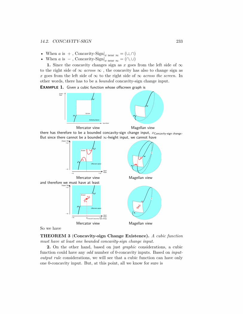
1. Since the concavity changes sign as x goes from the left side of ∞to the right side of ∞ across ∞ , the concavity has also to change sign asx goes from the left side of ∞ to the right side of ∞ across the screen. Inother words, there has to be a bounded concavity-sign change input.EXAMPLE 1. Given a cubic function whose offscreen graph is

Output Ruler

Input Ruler

Screen

Outlying Space

Mercator view Magellan viewthere has therefore to be a bounded concavity-sign change input, xConcavity-sign change.But since there cannot be a bounded ∞-height input, we cannot have

Output Ruler

Input Ruler

+∞–∞

+∞

–∞

Screen

Offscreen space

∞

Mercator view Magellan viewand therefore we must have at least

Output Ruler

Input Ruler+∞–∞

+∞

–∞

Screen

Offscreen space

Forced Concavity-sign changex

∞

Mercator view Magellan viewSo we haveTHEOREM 3 (Concavity-sign Change Existence). A cubic functionmust have at least one bounded concavity-sign change input.

2. On the other hand, based on just graphic considerations, a cubicfunction could have any odd number of 0-concavity inputs. Based on input-output rule considerations, we will see that a cubic function can have onlyone 0-concavity input. But, at this point, all we know for sure is


THEOREM 4 (0-Concavity Existence). A cubic functions must haveat least one concavity-sign change input and it is a 0-concavity input:

xConcavity-sign change = x0-concavity

14.3 Slope-sign

Given the cubic function CUBICa,b,c,d, that is the function specified by theglobal input-output rule


recall that when x is near ∞ the Slope-sign Near ∞ Theorem for cubicfunctions says that:• When a is + , Slope-Sign|x near ∞ = (�,�)• When a is − , Slope-Sign|x near ∞ = (�,�)

1. Since the slope does not changes sign as x goes through ∞ from theleft side of ∞ to the right side of ∞, the slope does not have to change signas x goes across the screen from the left side of ∞ to the right side of ∞ sothere does not have to be a bounded slope-sign change input:EXAMPLE 2. Given a cubic function whose offscreen graph is

Output Ruler

Input Ruler

Screen

Outlying Space

Mercator view Magellan viewthere is no need for a bounded slope-sign change input, xSlope-sign change and thereforewe can have

Output Ruler

Input Ruler

Screen

Outlying Space

Mercator view Magellan view2. On the other hand, based on just graphic considerations, a cubic

function could have any number of 0-slope inputs. Based on input-output

14.4. EXTREMUM 235

rule considerations, we will see that a cubic function can have only zero, oneor two 0-slope inputs. But, at this point, all we know for sure isTHEOREM 5 (Slope-Sign Change Existence). A cubic function neednot have a Slope-sign change input.And thus alsoTHEOREM 6 (0-Slope Existence). A cubic function need not have a0-Slope input.

14.4 Extremum

From the optimization viewpoint, the most immediately striking featureof an affine function is the absence of a forced extreme input, that is ofa bounded input whose output is either larger than the output of nearbyinputs or smaller than the output of nearby inputs. On the other hand, atthis point we cannot prove that there is no extreme input.EXAMPLE 3. Given a cubic function with the offscreen graph:

Output Ruler

Input Ruler

+∞–∞

+∞

–∞

Screen

Offscreen space

Since there can be no ∞-height input, we cannot have, for instance, either one of thefollowing

x∞-height

Output Ruler


+∞

–∞

Screen

Local minimum output

Local maximum output

x∞-height


Screen

Output Ruler+∞

–∞


On the other hand, there is nothing toprevent a fluctuation such as:


Screen

xmaxxmin

Output Ruler+∞

–∞

Local maximum output



But no extremum input is forced : Output Ruler


+∞

–∞

Screen

Offscreen space

So, we have

THEOREM 7 (Extremum Existence). A cubic function has no forcedextremum input

14.5 Height-sign

Given the cubic function CUBICa,b,c,d, that is the function specified by theglobal input-output rule


recall that when x is near∞ the Height-sign Near ∞ Theorem for cubicfunctions says that:• When a is + , Height-Sign|x near ∞ = (+,−)• When a is − , Height-Sign|x near ∞ = (−,+)

1. Since the height changes sign as x goes from the left side of ∞ to theright side of ∞ across ∞ , the height has also to change sign as x goes fromthe left side of ∞ to the right side of ∞ across the screen. In other words,there has to be a bounded height-sign change input.EXAMPLE 4. Given a cubic function whose offscreen graph is

Output Ruler

Input Ruler

Screen

Outlying Space

Mercator view Magellan viewthere has therefore to be a height-sign change input But since there cannot be a bounded∞-height input, we cannot have

14.6. 0-CONCAVITY LOCATION 237

Output Ruler

Input Ruler

+∞–∞

+∞

–∞

Screen

Offscreen space

∞

Mercator view Magellan viewand therefore we must have

Output Ruler


+∞

–∞

Screen

Offscreen space

Forced 0-Heightx

0 ∞

0

Mercator view Magellan view2. Moreover, because there is no bounded ∞-height input where the heightcould change sign, xheight-sign change has to be a bounded input where theheight is 0. As a result, we have thatTHEOREM 8 (Height-Sign Change Existence). A cubic functionsmust have a Height-sign change input and

xHeight-sign change = x0-height

LOCATION THEOREMSPreviously, we only established the existence of certain notable features ofcubic functions and this investigation was based on graphic considerations.Here we will investigate the location of the inputs where these notable fea-tures occur and this investigation will be based on input-output rule consid-erations.

14.6 0-Concavity LocationGiven a cubic function, the global problem of locating an input where thelocal concavity is 0 is still fairly simple.

More precisely, given a cubic function CUBICa,b,c,d, that is the cubicfunction specified by the global input-output rule



since the concavity near x0 is the local square coefficient 3ax0 + b, in orderto find the input(s) where the local concavity is 0, we need to solve the affineequation

3ax+ b = 0by reducing it to a basic equation:

3ax+ b −b = 0 −b3ax = −b3ax3a

= −b3a

x = −b3a

So, we have:

THEOREM 9 (0-slope Location). For any cubic function CUBICa,b,c,d,

x0−concavity = −b3a

In fact, we also have:

THEOREM 10 (Global Concavity-sign). Given a cubic function CUBICa,b,c,d,• When a is positive,

Concavity-sign CUBIC|Everywhere<−b3a= (∩,∩)

Concavity-sign CUBIC|−b3a

= (∩,∪)

Concavity-sign CUBIC|Everywhere>−b3a= (∪,∪)

• When a is negative,

Concavity-sign CUBIC|Everywhere<−b3a= (∪,∪)

Concavity-sign CUBIC|−b3a

= (∪,∩)

Concavity-sign CUBIC|Everywhere>−b3a= (∩,∩)

The case is easily made by testing near∞ the intervals for the correspondinginequations.

14.7. 0-SLOPE LOCATION 239

14.7 0-Slope Location

In the case of affine functions and of quadratic functions, we were able toprove that there was no shape difference with the principal term near ∞ byshowing that there could be no fluctuation:• In the case of affine functions we were able to prove that there was no

shape difference with dilation functions• In the case of quadratic functions we were able to prove that there was

no shape difference with square functions.More precisely, given the cubic function CUBICa,b,c,d, that is the functionspecified by the global input-output rule


since the slope near x0 is the local linear coefficient 3ax2 + 2bx+ c, in orderto find the input(s) where the local slope is 0, we need to solve the quadraticequation

3ax2 + 2bx+ c

which we have seen we cannot solve by reduction to a basic equation and forwhich we will have to use the 0-Height Theorem for quadratic functions,keeping in mind, though, that• For a as it appears in 0-Height Theorem for quadratic functions, we

have to substitute the squaring coefficient of 3ax2 + 2bx+ c, namely 3a,• For b as it appears in 0-Height Theorem for quadratic functions, we

have to substitute the linear coefficient of 3ax2 + 2bx+ c namely 2b,• For c as it appears in 0-Height Theorem for quadratic functions, we

have to substitute the constant coefficient of 3ax2 + 2bx+ c namely c.1. It will be convenient, keeping in mind the above substitutions, first

to compute

x0−slope for [3ax2+2bx+c] = − 2b2 · 3a

= − 2b6a

= − b3a= x0−concavity for CUBIC


Shape type O 2. Then, still keeping in mind the above substitutions, we compute thediscriminant of 3ax2 + 2bx+ c:

Discriminant[3ax2 + 2bx+ c] = (2b)2 − 4(3a)(c)= 4b2 − 12ac

3. Then we have:• When Discriminant [3ax2 +2bx+c] = 4b2−12ac < 0, the local linear co-

efficient of CUBIC, [3ax2 +2bx+c], has no 0-height input and thereforeCUBIC has no 0-slope input.

• When Discriminant [3ax2 + 2bx + c] = 4b2 − 12ac = 0, the local linearcoefficient of CUBIC, [3ax2 + 2bx + c], has one 0-height input andtherefore CUBIC has one 0-slope input, namely

I x0−slope for CUBIC = x0−height for [3ax2+2bx+c] = − b3a ,• When Discriminant [3ax2 + 2bx + c] = 4b2 − 12ac > 0, the local linear

coefficient of CUBIC, [3ax2 + 2bx + c], has two 0-height inputs andtherefore CUBIC has two 0-slope inputs., namely:

I x0−slope for CUBIC = x0−height for [3ax2+2bx+c] = − b3a+√

4b2−12ac2a

andI x0−slope for CUBIC = x0−height for [3ax2+2bx+c] = − b3a−

√4b2−12ac

2a

In terms of the function CUBIC, this gives us:

THEOREM 11 (0-slope Location). Given the cubic function CUBICa,b,c,d,when•Disc. [3ax2 + 2bx+ c] = 4b2 − 12ac < 0, CUBIC has no 0-Slope input•Disc. [3ax2 + 2bx+ c] = 4b2 − 12ac = 0, CUBIC has one 0-Slope input•Disc. [3ax2 + 2bx+ c] = 4b2 − 12ac > 0,CUBIC has two 0-Slope inputs

14.8 Extremum Location

The 0-slope inputs are the only ones which can be extremum inputs. So,there will therefore be three types of cubic functions according to the numberof 0-slopes inputs:

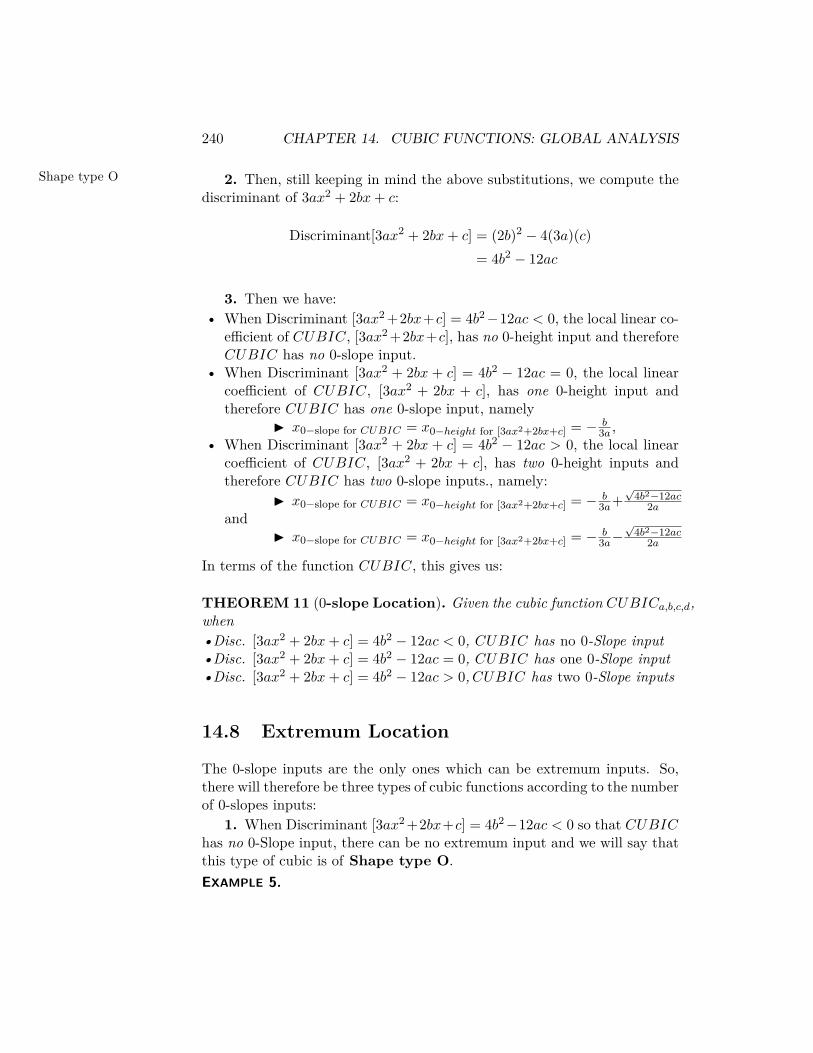
1. When Discriminant [3ax2 +2bx+c] = 4b2−12ac < 0 so that CUBIChas no 0-Slope input, there can be no extremum input and we will say thatthis type of cubic is of Shape type O.EXAMPLE 5.

14.8. EXTREMUM LOCATION 241

Shape type IShape type II

Output Ruler

Input Ruler

Screen

x0-concavity

Outlying Space+

–

Output Ruler

Input Ruler

Screen

x0-concavity

Outlying Space+

–

Cube coefficient positive Cube coefficient negative

Since cubic function of Shape type O have no 0-Slope input, their shape isnot like that of cubing functions.

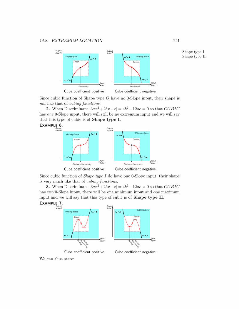
2. When Discriminant [3ax2 +2bx+c] = 4b2−12ac = 0 so that CUBIChas one 0-Slope input, there will still be no extremum input and we will saythat this type of cubic is of Shape type I.EXAMPLE 6.

Output Ruler

Input Ruler

Screen

x0-slope = x0-concavity

Outlying Space +

–

Output Ruler

Input Ruler

Screen

x0-slope = x0-concavity

Offscreen Space+

–


Since cubic function of Shape type I do have one 0-Slope input, their shapeis very much like that of cubing functions.

3. When Discriminant [3ax2 +2bx+c] = 4b2−12ac > 0 so that CUBIChas two 0-Slope input, there will be one minimum input and one maximuminput and we will say that this type of cubic is of Shape type II.EXAMPLE 7.

Output Ruler

Input Ruler

Screen

x0-concavity

Outlying Space +

–x0-slope

x0-slope

Output Ruler

Input Ruler

Screen

x0-concavity

Outlying Space+

–

x0-slope

x0-slope


We can thus state:


THEOREM 12 (Extremum Location). Given the cubic function CUBICa,b,c,d,when•Discriminant [3ax2 + 2bx + c] = 4b2 − 12ac < 0, CUBIC has no local

extremum input.•Discriminant [3ax2 + 2bx + c] = 4b2 − 12ac = 0, CUBIC has one

minimum-maximum input•Discriminant [3ax2 + 2bx+ c] = 4b2 − 12ac > 0, CUBIC has both

I xlocally minimum-output,I xlocally maximum-output,

THEOREM 13 (0-slope Location). Given the cubic function CUBICa,b,c,d,when•Disc. [3ax2 + 2bx+ c] = 4b2 − 12ac < 0, CUBIC has no 0-Slope input•Disc. [3ax2 + 2bx+ c] = 4b2 − 12ac = 0, CUBIC has one 0-Slope input•Disc. [3ax2 + 2bx+ c] = 4b2 − 12ac > 0,CUBIC has two 0-Slope inputs

14.9 0-Height LocationThe location of 0-height inputs in the case of a cubic function is usually noteasy.

1. So far, the situation has been as follows:i. The number of 0-height inputs for affine functions is always one,ii. The number of 0-height inputs for quadratic functions is already morecomplicated in that, depending on the sign of the extreme-output comparedwith the sign of the outputs for inputs near ∞, it can be none, one or two.It follows from the Extremum Location Theorem thatiii. The number of 0-height inputs for cubic functions depends

a. On the Shape type of the cubic function,b. In the case of Shape type II, on the sign of the extremum outputs

relative to the sign of the cubing coefficientEXAMPLE 8. The cubic function specified by the global graph

0

x0-output

Output Ruler

Input Ruler

Screen

Offscreen Space is of Shape Type O (No 0-slope input)and always has a single 0-height input.

EXAMPLE 9. The cubic function specified by the global graphs are all of the sameshape of Type II and the number of 0-height inputs depends on how high the graph is

14.9. 0-HEIGHT LOCATION 243

factorin relation to the 0-output level line.

x0-output

0

Output Ruler

Input Ruler

Screen

Offscreen Space

Output Ruler

Input Ruler

Screen

x0-output

0

x0-output

Offscreen Space

x0-output

0

x0-outputx0-output

Output Ruler

Input Ruler

Screen

Offscreen Space

2. The obstruction to computing the solutions that we encountered whentrying to solve quadratic equations, namely that there was one more termthan an equation has sides is even worse here since we have four terms andan equation still has only two sides.There does happen to be a procedure, using two successive localizations,to get rid of the two middle terms, but it turns out that it is so compli-cated that it is essentially useless for our purposes. Moreover, while thisapproach would still work for polynomial functions of degree 4, it breaksdown completely with polynomial functions of degree 5.

In 1824, to the surprise of many mathematicians of the time, a youngNorwegian mathematician, Abel, proved that the approach could not workfor all polynomial functions of degree 5 and, therefore, that there could notbe any such thing as a “quintic formula” for polynomial functions of degree 5.Abel accomplished this by giving a procedure that, from any such “quinticformula”, would give a proof that “1=2”. Then, around 1830, Galois, aneven younger French mathematician, extended this “negative result” to allpolynomial functions of degree larger than 5.So, one normally uses so-called “approximative numerical methods” butthese are quite outside the scope of this text

3. There is one case where we can easily find x0−height for a cubic func-tion and that is when it happens that, by some miracle, we are able tofactor it. But there is no more procedure for factoring cubics than there isfor factoring quadratics and, in the fact the only sure way to factor quadrat-ics or cubics is first to solve the corresponding equation. So, the real miracleis when the input-output rule comes already “factored”.

Cubic Functions: Global Analysis - Free Math...

Documents

Transcript of Cubic Functions: Global Analysis - Free Math...