
CSE544: Principles of Database Systems
26
CSE544: Principles of Database Systems Database Statistics CSE544 - Spring, 2012 1
Transcript of CSE544: Principles of Database Systems
CSE544: Principles of Database Systems
Database Statistics
CSE544 - Spring, 2012 1
Announcement
• Paper review was due today: – Will have a short discussion on Monday, 4/23
• Map/Reduce paper review: – Due Wednesday, 4/25
• Project proposals – Due Sunday, 4/22
CSE544 - Spring, 2012 2
Outline
• Chapter 15 in the textbook
• Paper on selectivity of conjuncts – Will have a short discussion on Monday
CSE544 - Spring, 2012 3
CSE544 - Spring, 2012 4
Query Optimization
Three major components:
1. Search space
2. Algorithm for enumerating query plans
3. Cardinality and cost estimation
CSE544 - Spring, 2012 5
3. Cardinality and Cost Estimation
• Collect statistical summaries of stored data
• Estimate size (=cardinality) in a bottom-up fashion – This is the most difficult part, and still inadequate
in today’s query optimizers • Estimate cost by using the estimated size
– Hand-written formulas, similar to those we used for computing the cost of each physical operator
CSE544 - Spring, 2012 6
Statistics on Base Data
• Collected information for each relation – Number of tuples (cardinality) – Indexes, number of keys in the index – Number of physical pages, clustering info – Statistical information on attributes
• Min value, max value, number distinct values • Histograms
– Correlations between columns (hard)
• Collection approach: periodic, using sampling
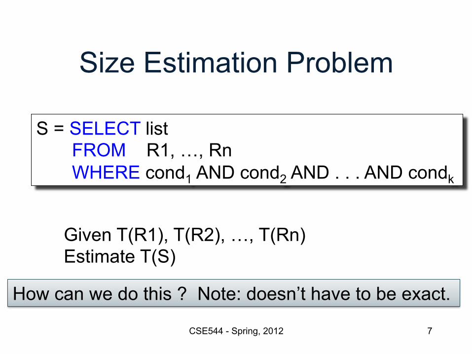
Size Estimation Problem
CSE544 - Spring, 2012 7
S = SELECT list FROM R1, …, Rn WHERE cond1 AND cond2 AND . . . AND condk
Given T(R1), T(R2), …, T(Rn) Estimate T(S)
How can we do this ? Note: doesn’t have to be exact.
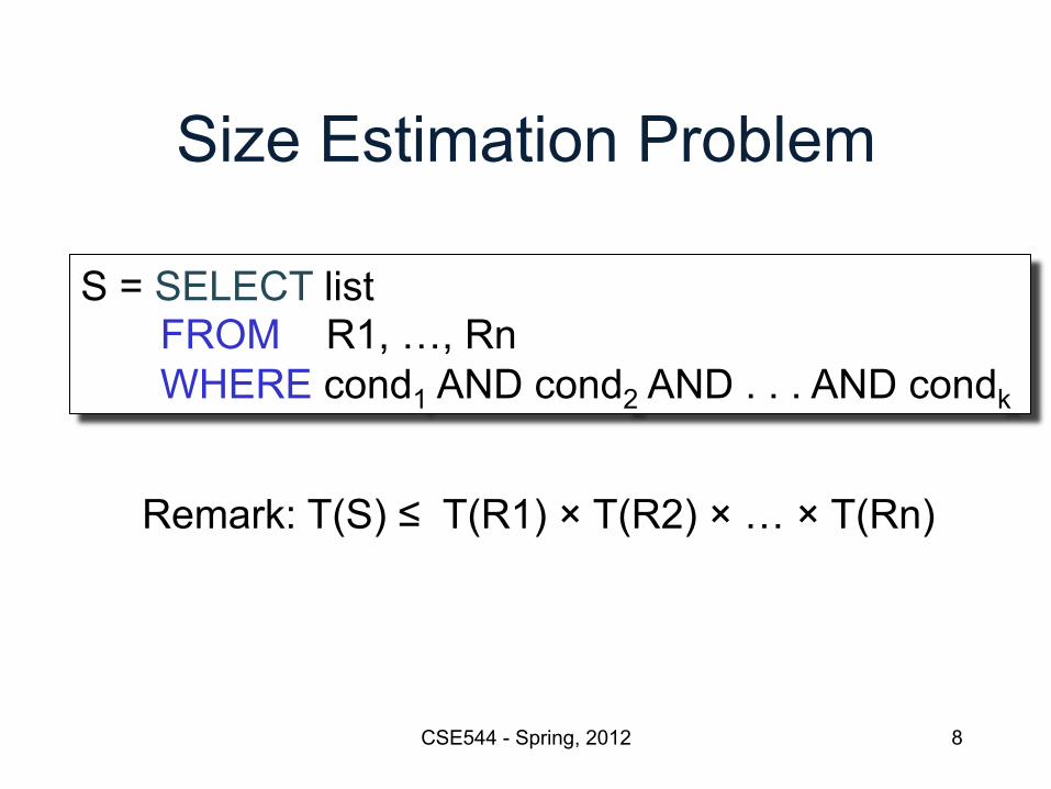
Size Estimation Problem
CSE544 - Spring, 2012 8
Remark: T(S) ≤ T(R1) × T(R2) × … × T(Rn)
S = SELECT list FROM R1, …, Rn WHERE cond1 AND cond2 AND . . . AND condk
Selectivity Factor
• Each condition cond reduces the size by some factor called selectivity factor
• Assuming independence, multiply the selectivity factors
CSE544 - Spring, 2012 9
Example
CSE544 - Spring, 2012 10
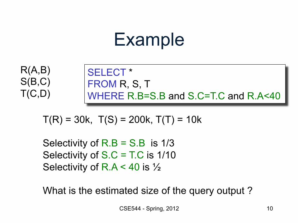
SELECT * FROM R, S, T WHERE R.B=S.B and S.C=T.C and R.A<40
R(A,B) S(B,C) T(C,D)
T(R) = 30k, T(S) = 200k, T(T) = 10k Selectivity of R.B = S.B is 1/3 Selectivity of S.C = T.C is 1/10 Selectivity of R.A < 40 is ½ What is the estimated size of the query output ?
Rule of Thumb
• If selectivities are unknown, then: selectivity factor = 1/10 [System R, 1979]
CSE544 - Spring, 2012 11
12
Using Data Statistics
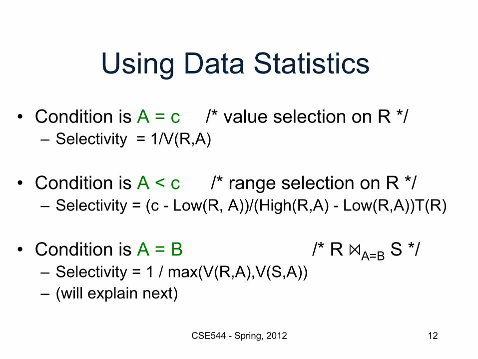
• Condition is A = c /* value selection on R */ – Selectivity = 1/V(R,A)
• Condition is A < c /* range selection on R */ – Selectivity = (c - Low(R, A))/(High(R,A) - Low(R,A))T(R)
• Condition is A = B /* R ⨝A=B S */ – Selectivity = 1 / max(V(R,A),V(S,A)) – (will explain next)
CSE544 - Spring, 2012
13
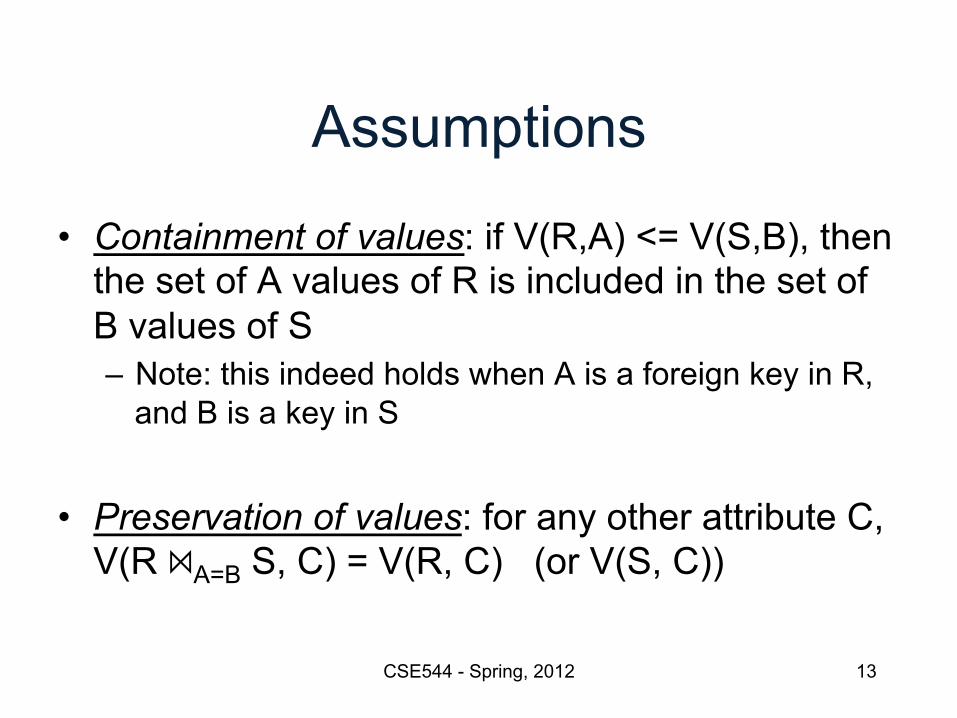
Assumptions
• Containment of values: if V(R,A) <= V(S,B), then the set of A values of R is included in the set of B values of S – Note: this indeed holds when A is a foreign key in R,
and B is a key in S
• Preservation of values: for any other attribute C, V(R ⨝A=B S, C) = V(R, C) (or V(S, C))
CSE544 - Spring, 2012
14
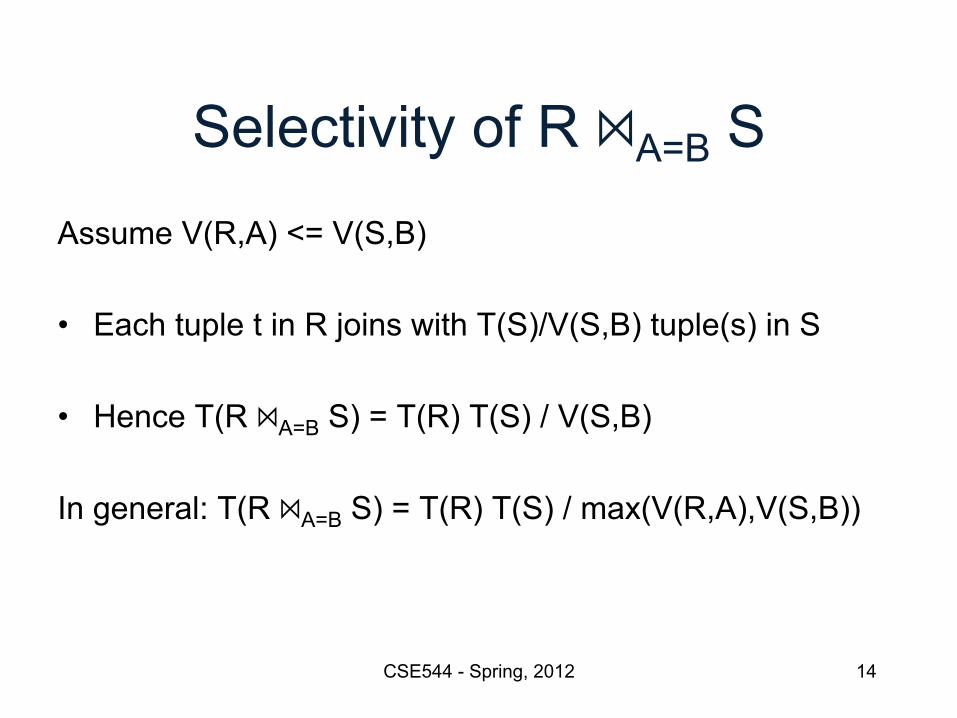
Selectivity of R ⨝A=B S Assume V(R,A) <= V(S,B)
• Each tuple t in R joins with T(S)/V(S,B) tuple(s) in S
• Hence T(R ⨝A=B S) = T(R) T(S) / V(S,B)
In general: T(R ⨝A=B S) = T(R) T(S) / max(V(R,A),V(S,B))
CSE544 - Spring, 2012
15
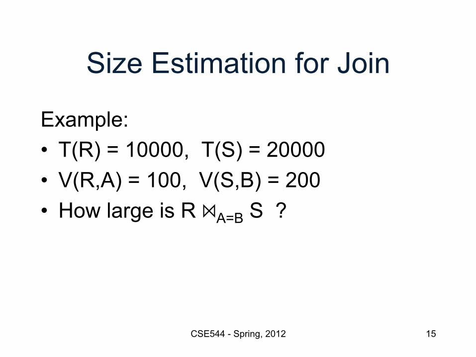
Size Estimation for Join
Example: • T(R) = 10000, T(S) = 20000 • V(R,A) = 100, V(S,B) = 200 • How large is R ⨝A=B S ?
CSE544 - Spring, 2012
16
Histograms
• Statistics on data maintained by the RDBMS
• Makes size estimation much more accurate (hence, cost estimations are more accurate)
CSE544 - Spring, 2012
Histograms
CSE544 - Spring, 2012 17
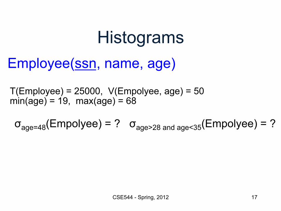
Employee(ssn, name, age)
T(Employee) = 25000, V(Empolyee, age) = 50 min(age) = 19, max(age) = 68
σage=48(Empolyee) = ? σage>28 and age<35(Empolyee) = ?
Histograms
CSE544 - Spring, 2012
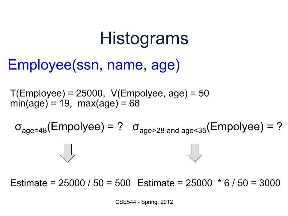
Employee(ssn, name, age)
T(Employee) = 25000, V(Empolyee, age) = 50 min(age) = 19, max(age) = 68
Estimate = 25000 / 50 = 500 Estimate = 25000 * 6 / 50 = 3000
σage=48(Empolyee) = ? σage>28 and age<35(Empolyee) = ?
Histograms
CSE544 - Spring, 2012
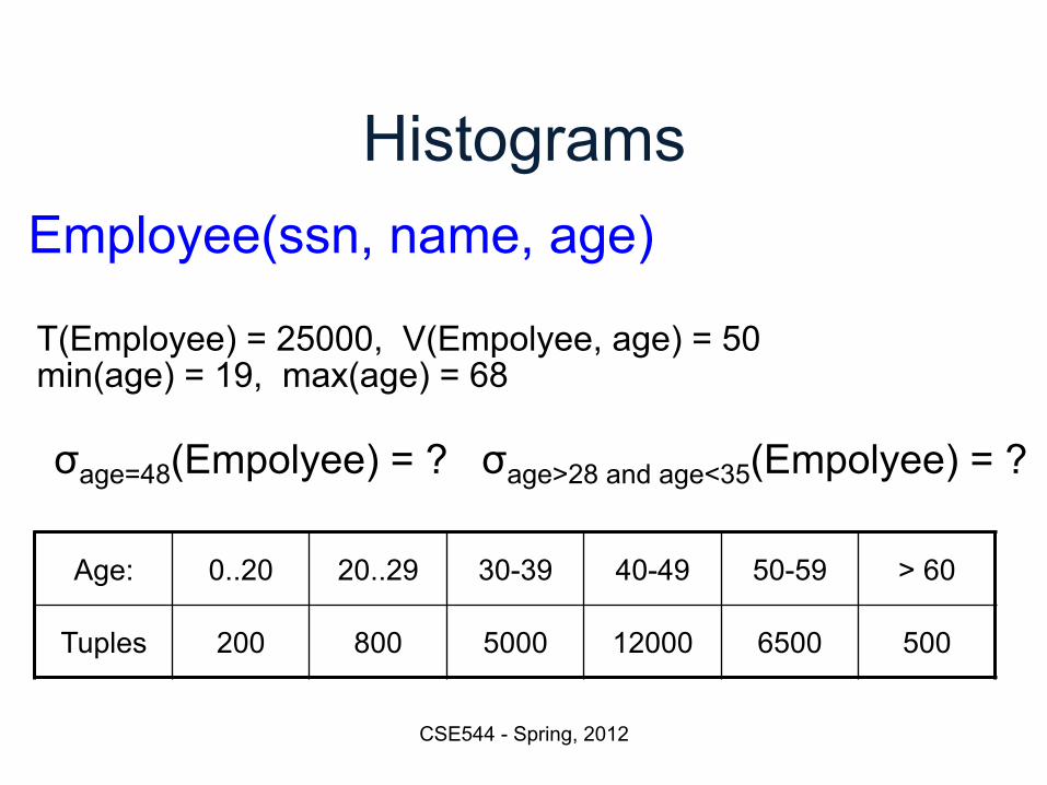
Age: 0..20 20..29 30-39 40-49 50-59 > 60
Tuples 200 800 5000 12000 6500 500
Employee(ssn, name, age)
T(Employee) = 25000, V(Empolyee, age) = 50 min(age) = 19, max(age) = 68
σage=48(Empolyee) = ? σage>28 and age<35(Empolyee) = ?
Histograms Employee(ssn, name, age)
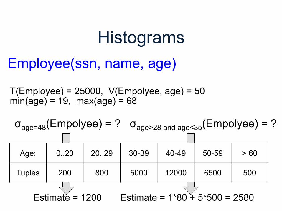
T(Employee) = 25000, V(Empolyee, age) = 50 min(age) = 19, max(age) = 68
Estimate = 1200 Estimate = 1*80 + 5*500 = 2580
Age: 0..20 20..29 30-39 40-49 50-59 > 60
Tuples 200 800 5000 12000 6500 500
σage=48(Empolyee) = ? σage>28 and age<35(Empolyee) = ?

Types of Histograms
• How should we determine the bucket boundaries in a histogram ?
CSE544 - Spring, 2012 21
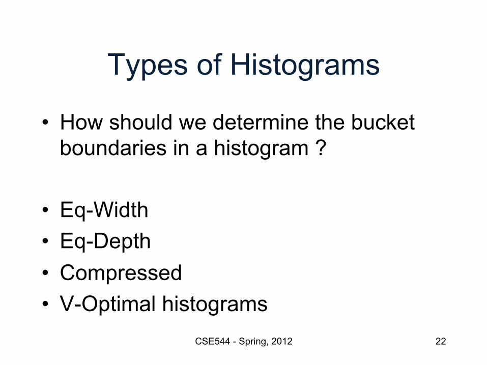
Types of Histograms
• How should we determine the bucket boundaries in a histogram ?
• Eq-Width • Eq-Depth • Compressed • V-Optimal histograms
CSE544 - Spring, 2012 22
Histograms
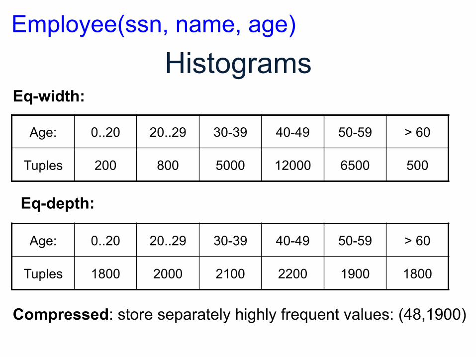
Age: 0..20 20..29 30-39 40-49 50-59 > 60
Tuples 200 800 5000 12000 6500 500
Employee(ssn, name, age)
Age: 0..20 20..29 30-39 40-49 50-59 > 60
Tuples 1800 2000 2100 2200 1900 1800
Eq-width:
Eq-depth:
Compressed: store separately highly frequent values: (48,1900)
V-Optimal Histograms
• Defines bucket boundaries in an optimal way, to minimize the error over all point queries
• Computed rather expensively, using dynamic programming
• Modern databases systems use V-optimal histograms or some variations
CSE544 - Spring, 2012 24
Difficult Questions on Histograms
• Small number of buckets – Hundreds, or thousands, but not more – WHY ?
• Not updated during database update, but recomputed periodically – WHY ?
• Multidimensional histograms rarely used – WHY ?
CSE544 - Spring, 2012 25
Summary of Query Optimization
• Three parts: – search space, algorithms, size/cost estimation
• Ideal goal: find optimal plan. But – Impossible to estimate accurately – Impossible to search the entire space
• Goal of today’s optimizers: – Avoid very bad plans
CSE544 - Spring, 2012 26


