CSE373: Data Structures & Algorithms

Lecture 12: Amortized Analysis and Memory Locality

Lauren Milne

Summer 2015

2

Announcements

• Midterms graded, pick them up at the end of class.

• Homework 3 due on Wednesday at 11pm

• TA Session tomorrow starts at 11 AM (not 10:50 AM)

3

Amortized Analysis

• In amortized analysis, the time required to perform a sequence of data structure operations is averaged over all the operations performed.

• Typically used to show that the average cost of an operation is small for a sequence of operations, even though a single operation can cost a lot

4

Amortized Analysis

• Recall our plain-old stack implemented as an array that doubles its size if it runs out of room– Can we claim push is O(1) time if resizing is O(n) time?– We can’t, but we can claim it’s an O(1) amortized operation

5

Amortized Complexity

We get an upperbound T(n) on the total time of a sequence of n operations. The average time per operation is then T(n)/n, which is also the amortized time per operation.

If a sequence of n operations takes O(n f(n)) time, we say the amortized runtime is O(f(n))

– If n operations take O(n), what is amortized time per operation?• O(1) per operation

– If n operations take O(n3), what is amortized time per operation?• O(n2) per operation

The worst case time for an operation can be larger than f(n), but amortized guarantee ensures the average time per operation for any sequence is O(f(n))

6

“Building Up Credit”

• Can think of preceding “cheap” operations as building up “credit” that can be used to “pay for” later “expensive” operations

• Because any sequence of operations must be under the bound, enough “cheap” operations must come first– Else a prefix of the sequence would violate the bound

7

Example #1: Resizing stack

A stack implemented with an array where we double the size of the array if it becomes full

Claim: Any sequence of push/pop/isEmpty is amortized O(1) per operation

Need to show any sequence of M operations takes time O(M)– Recall the non-resizing work is O(M) (i.e., M*O(1))– The resizing work is proportional to the total number of element

copies we do for the resizing– So it suffices to show that:

After M operations, we have done < 2M total element copies

(So average number of copies per operation is bounded by a constant)

8

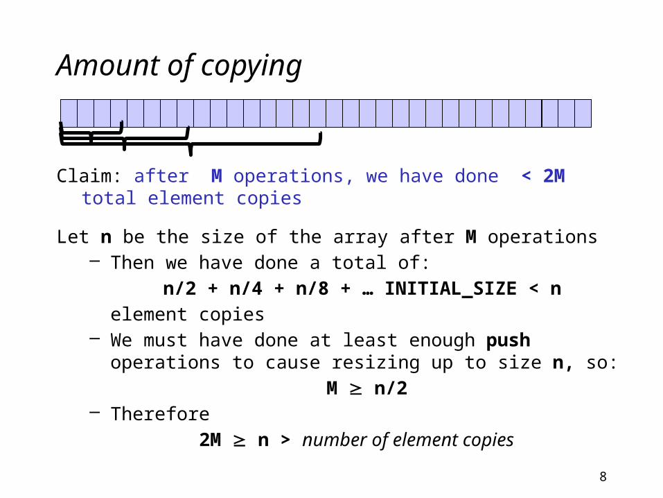
Amount of copying

Claim: after M operations, we have done < 2M total element copies

Let n be the size of the array after M operations– Then we have done a total of:

n/2 + n/4 + n/8 + … INITIAL_SIZE < nelement copies

– We must have done at least enough push operations to cause resizing up to size n, so:

M n/2– Therefore

2M n > number of element copies

9

Other approaches

• If array grows by a constant amount (say 1000),

operations are not amortized O(1)

– After O(M) operations, you may have done (M2) copies

• If array shrinks when 1/2 empty, operations are not amortized O(1)– Terrible case: pop once and shrink, push once and grow, pop

once and shrink, …

• If array shrinks when 3/4 empty, it is amortized O(1)– Proof is more complicated, but basic idea remains: by the time

an expensive operation occurs, many cheap ones occurred

10

Example #2: Queue with two stacks

A clever and simple queue implementation using only stacks

class Queue<E> { Stack<E> in = new Stack<E>(); Stack<E> out = new Stack<E>(); void enqueue(E x){ in.push(x); } E dequeue(){ if(out.isEmpty()) { while(!in.isEmpty()) { out.push(in.pop()); } } return out.pop(); }}

CBA

in out

enqueue: A, B, C

11

Example #2: Queue with two stacks

A clever and simple queue implementation using only stacks

class Queue<E> { Stack<E> in = new Stack<E>(); Stack<E> out = new Stack<E>(); void enqueue(E x){ in.push(x); } E dequeue(){ if(out.isEmpty()) { while(!in.isEmpty()) { out.push(in.pop()); } } return out.pop(); }}

in out

dequeue

BC

A

12

Example #2: Queue with two stacks

A clever and simple queue implementation using only stacks

class Queue<E> { Stack<E> in = new Stack<E>(); Stack<E> out = new Stack<E>(); void enqueue(E x){ in.push(x); } E dequeue(){ if(out.isEmpty()) { while(!in.isEmpty()) { out.push(in.pop()); } } return out.pop(); }}

in out

enqueue D, E

BC

A

ED

13

Example #2: Queue with two stacks

A clever and simple queue implementation using only stacks

class Queue<E> { Stack<E> in = new Stack<E>(); Stack<E> out = new Stack<E>(); void enqueue(E x){ in.push(x); } E dequeue(){ if(out.isEmpty()) { while(!in.isEmpty()) { out.push(in.pop()); } } return out.pop(); }}

in out

dequeue twice

C B A

ED

14

Example #2: Queue with two stacks

A clever and simple queue implementation using only stacks

class Queue<E> { Stack<E> in = new Stack<E>(); Stack<E> out = new Stack<E>(); void enqueue(E x){ in.push(x); } E dequeue(){ if(out.isEmpty()) { while(!in.isEmpty()) { out.push(in.pop()); } } return out.pop(); }}

in out

dequeue again

D C B A

E

15

Analysis

• dequeue is not O(1) worst-case because out might be empty and in may have lots of items

• But if the stack operations are (amortized) O(1), then any sequence of queue operations is amortized O(1)

– The total amount of work done per element is 1 push onto in, 1 pop off of in, 1 push onto out, 1 pop off of out

– When you reverse n elements, there were n earlier O(1) enqueue operations to average with

16

When is Amortized Analysis Useful?

• When the average per operation is all we care about (i.e., sum over all operations), amortized is perfectly fine

• If we need every operation to finish quickly (e.g., in a web server), amortized bounds may be too weak

17

Not always so simple

• Proofs for amortized bounds can be much more complicated

• Example: Splay trees are dictionaries with amortized O(log n) operations– See Chapter 4.5 if curious

• For more complicated examples, the proofs need much more sophisticated invariants and “potential functions” to describe how earlier cheap operations build up “energy” or “money” to “pay for” later expensive operations– See Chapter 11 if curious

• But complicated proofs have nothing to do with the code (which may be easy!)

18

Switching gears…

• Memory hierarchy/locality

19

Why do we need to know about the memory hierarchy/locality?

• One of the assumptions that Big-O makes is that all operations take the same amount of time

• Is this really true?

20

Definitions

• A cycle (for our purposes) is the time it takes to execute a single simple instruction (e.g. adding two registers together)

• Memory latency is the time it takes to access memory

21

CPU~16-64+ registers

Time to access:

1 ns per instruction

CacheSRAM

8 KB - 4 MB2-10 ns

Main Memory

DRAM

2-10 GB40-100 ns

Disk

many GB

a fewmilliseconds

(5-10 million ns)

22

What does this mean?

• It is much faster to do: Than:

5 million arithmetic ops 1 disk access

2500 L2 cache accesses 1 disk access

400 main memory accesses 1 disk access• Why are computers build this way?

– Physical realities (speed of light, closeness to CPU)– Cost (price per byte of different storage technologies)– Under the right circumstances, this kind of hierarchy can

simulate storage with access time of highest (fastest) level and size of lowest (largest) level

23

24

Processor-Memory Performance Gap

25

What can be done?

• Goal: attempt to reduce the accesses to slower levels

26

So, what can we do?

• The hardware automatically moves data from main memory into the caches for you– Replacing items already there– Algorithms are much faster if “data fits in cache” (often does)

• Disk accesses are done by software (e.g. ask operating system to open a file or database to access some records)

• So most code “just runs,” but sometimes it’s worth designing algorithms / data structures with knowledge of memory hierarchy– To do this, we need to understand locality

27

Locality

• Temporal Locality (locality in time)– If an item (a location in memory) is referenced, that same

location will tend to be referenced again soon.

• Spatial Locality (locality in space)– If an item is referenced, items whose addresses are close

by tend to be referenced soon.

28

How does data move up the hierarchy?

• Moving data up the hierarchy is slow because of latency (think distance to travel)– Since we’re making the trip anyway, might as well carpool

• Get a block of data in the same time we could get a byte– Sends nearby memory because

• It’s easy• Likely to be asked for soon (think fields/arrays)

• Once a value is in cache, may as well keep it around for a while; accessed once, a value is more likely to be accessed again in the near future (as opposed to some random other value)

Spatial Locality

Temporal Locality

29

Cache Facts

• Definitions:– Cache hit – address requested is in the cache– Cache miss – address requested is NOT in the

cache– Block or page size – the number of contiguous

bytes moved from disk to memory– Cache line size – the number of contiguous bytes

moved from memory to cache

30

Examples

x = a + 6

y = a + 5

z = 8 * a

miss

hit

hit

31

Examples

x = a + 6

y = a + 5

z = 8 * a

x = a[0] + 6

y = a[1] + 5

z = 8 * a[2]

miss miss

hit

hit

hit

hit

32

Examples

x = a + 6

y = a + 5

z = 8 * a

x = a[0] + 6

y = a[1] + 5

z = 8 * a[2]

miss miss

hit

hit

hit

hit

temporal locality

spatiallocality

33

Locality and Data Structures

• Which has (at least the potential) for better spatial locality, arrays or linked lists?

34

Locality and Data Structures

• Which has (at least the potential) for better spatial locality, arrays or linked lists?– e.g. traversing elements

• Only miss on first item in a cache line

cache line size cache line size

miss misshit hit hit hit hit

35

Locality and Data Structures

• Which has (at least the potential) for better spatial locality, arrays or linked lists?– e.g. traversing elements

36

Locality and Data Structures

• Which has (at least the potential) for better spatial locality, arrays or linked lists?– e.g. traversing elements

• Miss on every item (unless more than one randomly happen to be in the same cache line)

miss hit miss hit miss hit miss hit