CSCI-GA.3033-018 - Geometric Modeling - Spring 17 ...panozzo/gp18/Handout1.pdf · Check out...
6
CSCI-GA.3033-018 - Geometric Modeling - Spring 17 Assignment 1: Hello World In this exercise you will • Familiarize yourself with libigl and the provided mesh viewer. • Get acquainted with some basic mesh programming by evaluating surface normals, computing mesh connectivity and isolating connected components. • Implement a simple mesh subdivision scheme. 1. First steps with libigl The first task is to familiarize yourself with some of the basic code infrastructure provided by libigl. 1.1. Eigen. libigl uses the Eigen library for all of its matrix computations. In libigl, a mesh is typically represented by a set of two Eigen arrays, V and F. V is a float or double array (dimension #V × 3 where #V is the number of vertices) that contains the positions of the vertices of the mesh, where the i-th row of V contains the coordinates of the i-th vertex. F is an integer array (dimension #faces × 3 where #F is the number of faces) which contains the descriptions of the triangles in the mesh. The i-th row of F contains the indices of the vertices in V that form the i-th face, ordered counter-clockwise. Check out the ”Getting Started” page of Eigen as well as the Quick Reference page to acquaint yourselves with the basic matrix operations supported. Note that you need not install Eigen manually since a reasonably up-to-date version is included as a submodule in libigl. 1.2. Installing libigl and Running the Tutorials. If you haven’t already, install libigl by following the instructions in the “General Rules and Instructions” handout. Next, build the tutorials: cd $LIBIGL ROOT/tutorial; mkdir build; cd build; cmake ..; make -j2. This can take a while, so be sure to set the ”-j” flag to run on as many cores as possible. Each tutorial is named with format XXX TUTORIAL NAME, where XXX is the number ID of the tutorial. After the build completes, each tutorial executable can be run, e.g.: ./XXX TUTORIAL NAME bin The source code for the corresponding tutorial is located in $LIBIGL ROOT/tutorial/XXX TUTORIAL NAME/main.cpp Experiment with the basic functionality of libigl and the included mesh viewer by running at least the first 6 tutorials and inspecting the corresponding source code. 2. Neighborhood Computations For this task, you will use libigl to perform basic neighborhood computations on a mesh. Computing the neighbors of a mesh face or vertex is required for most mesh processing operations, as you will see later in the class. For this task, you need to fill in the appropriate sections (inside the keyboard callback, keys ’1’ to ’2’) of src/main.cpp to compute the neighborhood relations using libigl. In order to use a function from libigl (e.g. the function to compute per-face normals), you must include the relevant Daniele Panozzo January 30, 2018 1
Transcript of CSCI-GA.3033-018 - Geometric Modeling - Spring 17 ...panozzo/gp18/Handout1.pdf · Check out...

CSCI-GA.3033-018 - Geometric Modeling - Spring 17
Assignment 1: Hello WorldIn this exercise you will
• Familiarize yourself with libigl and the provided mesh viewer.• Get acquainted with some basic mesh programming by evaluating surface normals, computing
mesh connectivity and isolating connected components.• Implement a simple mesh subdivision scheme.
1. First steps with libigl
The first task is to familiarize yourself with some of the basic code infrastructure provided by libigl.
1.1. Eigen. libigl uses the Eigen library for all of its matrix computations. In libigl, a mesh istypically represented by a set of two Eigen arrays, V and F. V is a float or double array (dimension #V× 3 where #V is the number of vertices) that contains the positions of the vertices of the mesh, wherethe i-th row of V contains the coordinates of the i-th vertex. F is an integer array (dimension #faces ×3 where #F is the number of faces) which contains the descriptions of the triangles in the mesh. Thei-th row of F contains the indices of the vertices in V that form the i-th face, ordered counter-clockwise.
Check out the ”Getting Started” page of Eigen as well as the Quick Reference page to acquaintyourselves with the basic matrix operations supported.
Note that you need not install Eigen manually since a reasonably up-to-date version is included as asubmodule in libigl.
1.2. Installing libigl and Running the Tutorials. If you haven’t already, install libigl by followingthe instructions in the “General Rules and Instructions” handout. Next, build the tutorials:cd $LIBIGL ROOT/tutorial; mkdir build; cd build; cmake ..; make -j2.This can take a while, so be sure to set the ”-j” flag to run on as many cores as possible.
Each tutorial is named with format XXX TUTORIAL NAME, where XXX is the number ID of the tutorial.After the build completes, each tutorial executable can be run, e.g.: ./XXX TUTORIAL NAME bin
The source code for the corresponding tutorial is located in$LIBIGL ROOT/tutorial/XXX TUTORIAL NAME/main.cpp
Experiment with the basic functionality of libigl and the included mesh viewer by running at leastthe first 6 tutorials and inspecting the corresponding source code.
2. Neighborhood Computations
For this task, you will use libigl to perform basic neighborhood computations on a mesh. Computingthe neighbors of a mesh face or vertex is required for most mesh processing operations, as you will seelater in the class. For this task, you need to fill in the appropriate sections (inside the keyboard callback,keys ’1’ to ’2’) of src/main.cpp to compute the neighborhood relations using libigl. In order to usea function from libigl (e.g. the function to compute per-face normals), you must include the relevant
Daniele PanozzoJanuary 30, 2018
1
CSCI-GA.3033-018 - Geometric Modeling - Spring 17
header file at the top of your main.cpp file (e.g. #include <igl/per face normals.h>) and call itlater in your code (igl::per face normals(V,F,FN)).
2.1. Vertex-to-Face Relations. Given V and F, generate an adjacency list which contains, for eachvertex, a list of faces adjacent to it. The ordering of the faces incident on a vertex does not matter.Your program should print out the vertex-to-face relations in text form when key ’1’ is pressed.
Relevant libigl functions: igl::vertex triangle adjacency.
2.2. Vertex-to-Vertex Relations. Given V and F, generate an adjacency list which contains, for eachvertex, a list of vertices connected with it. Two vertices are connected if there exists an edge betweenthem, i.e., if the two vertices appear in the same row of F. The ordering of the vertices in each list doesnot matter. Your program should print out the vertex-to-vertex relations in text form when key ’2’ ispressed.
Relevant libigl functions: igl::adjacency list.
2.3. Visualizing the Neighborhood Relations. Check your results by comparing them to the built-inrelations calculated by the mesh viewer. You can do this by clicking on the checkboxes “Show vertexlabels” and “Show faces labels” in the viewer window.
Required output of this section:
• A text dump of the content of the two data structures for the provided mesh “plane.off”.
3. Shading
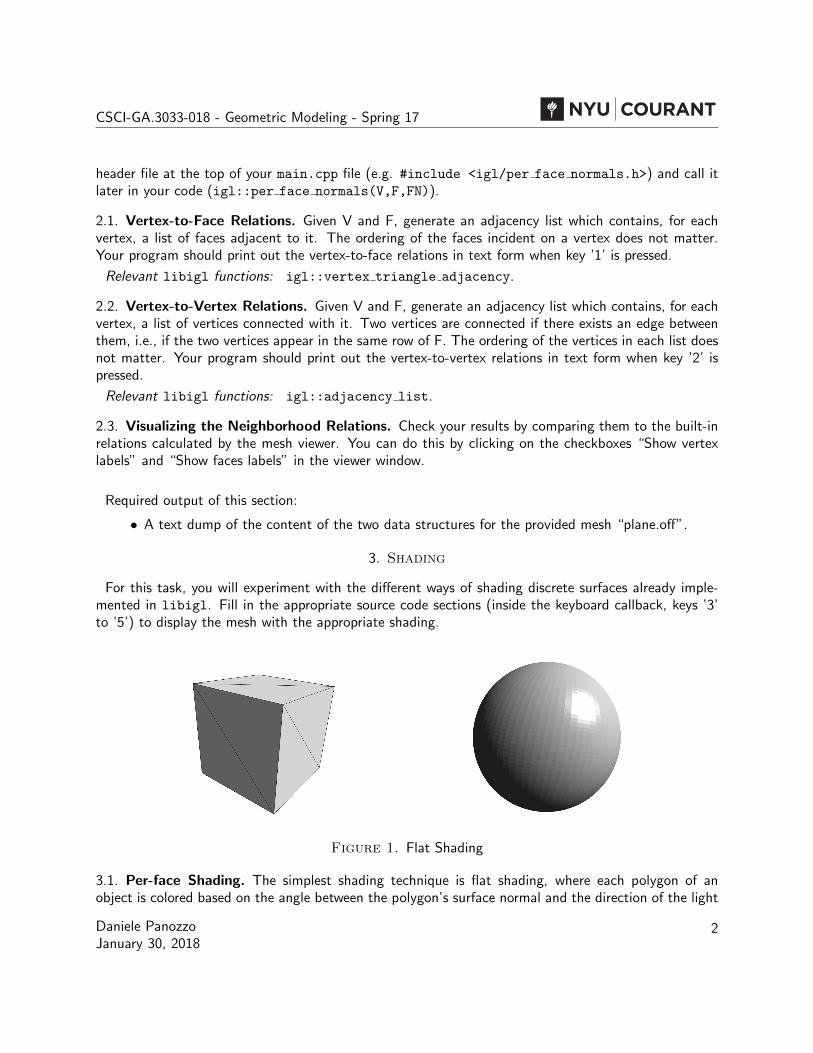
For this task, you will experiment with the different ways of shading discrete surfaces already imple-mented in libigl. Fill in the appropriate source code sections (inside the keyboard callback, keys ’3’to ’5’) to display the mesh with the appropriate shading.
Figure 1. Flat Shading
3.1. Per-face Shading. The simplest shading technique is flat shading, where each polygon of anobject is colored based on the angle between the polygon’s surface normal and the direction of the light
Daniele PanozzoJanuary 30, 2018
2

CSCI-GA.3033-018 - Geometric Modeling - Spring 17
source, their respective colors, and the intensity of the light source. With flat shading, all vertices ofa polygon are colored identically. Your program should compute the appropriate shading normals andshade the input mesh with flat shading when the key ’3’ is pressed.
Relevant libigl functions: igl::per face normals. Call viewer.data.set normals(·) to setthe shading in the viewer to use the normals you computed.
3.2. Per-vertex Shading. Flat shading may produce visual artifacts, due to the color discontinuitybetween neighboring faces. Specular highlights may be rendered poorly with flat shading. When per-vertex shading is used, per-vertex normals are computed for each vertex by averaging the normals ofthe surrounding faces. Your program should compute the appropriate shading normals and shade theinput mesh with per-vertex shading when the key ’4’ is pressed.
Relevant libigl functions: igl::per vertex normals. Call viewer.data.set normals(·) toset the shading in the viewer to use the normals you computed.
Compare the result must be compared with the one obtained with flat shading.
Figure 2. Per-Vertex Shading
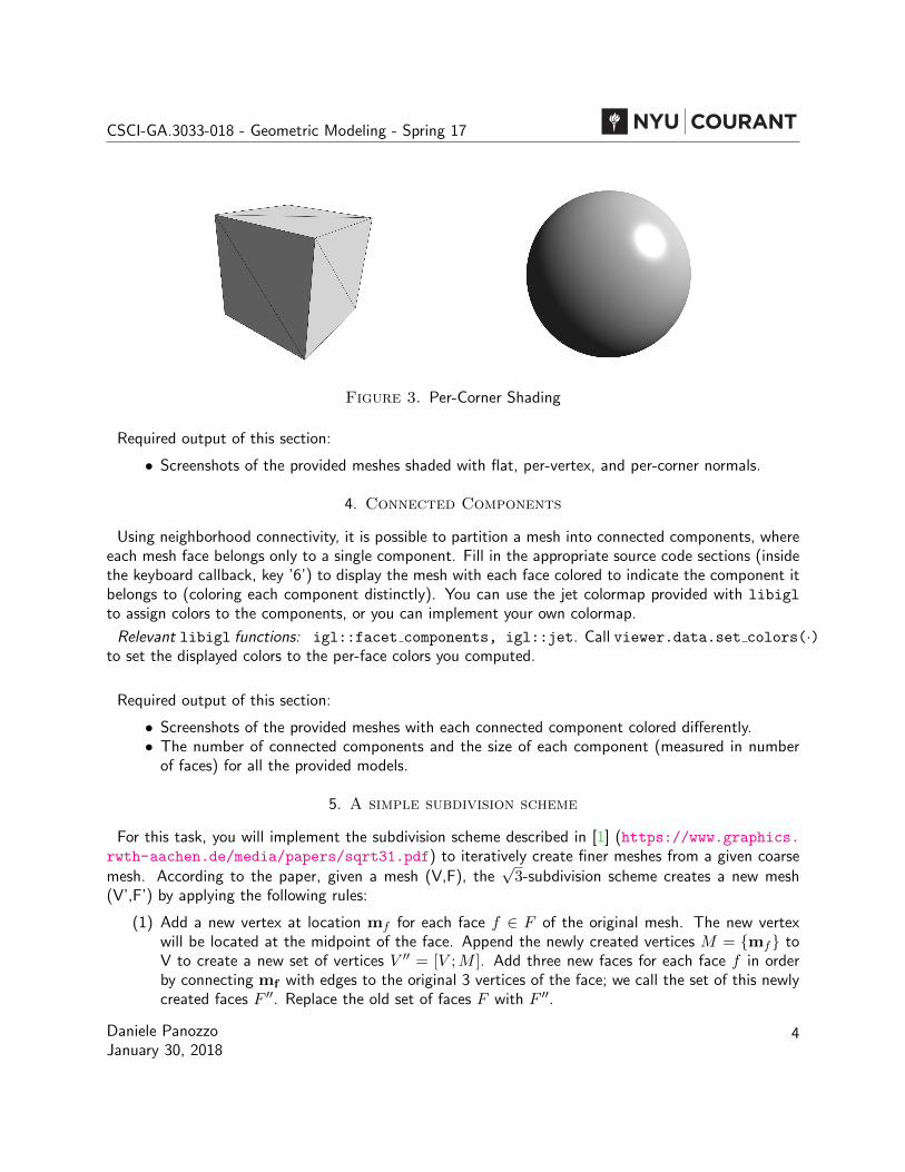
3.3. Per-corner Shading. On models with sharp feature lines, averaging the per-face normals on thefeature, as done for per-vertex shading, may result in blurred rendering. It is possible to avoid thislimitation and to render crisp sharp features by using per-corner normals. In this case, a different normalis assigned to each face corner; this implies that every vertex will get a (possibly different) normalfor every adjacent face. A threshold parameter is used to decide when an edge belongs to a sharpfeature. The threshold is applied to the angle between the two corner normals: if it is less than thethreshold value, the normals must be averaged, otherwise they are kept untouched. Your program shouldcompute the appropriate shading normals (with a threshold of your choice) and shade the input meshwith per-vertex shading when the key ’5’ is pressed.
Relevant libigl functions: igl::per corner normals. Call viewer.data.set normals(·) toset the shading in the viewer to use the normals you computed.
Compare the result must be compared with the one obtained with flat and per-vertex shading. Exper-iment with the threshold value.
Daniele PanozzoJanuary 30, 2018
3
CSCI-GA.3033-018 - Geometric Modeling - Spring 17
Figure 3. Per-Corner Shading
Required output of this section:
• Screenshots of the provided meshes shaded with flat, per-vertex, and per-corner normals.
4. Connected Components
Using neighborhood connectivity, it is possible to partition a mesh into connected components, whereeach mesh face belongs only to a single component. Fill in the appropriate source code sections (insidethe keyboard callback, key ’6’) to display the mesh with each face colored to indicate the component itbelongs to (coloring each component distinctly). You can use the jet colormap provided with libigl
to assign colors to the components, or you can implement your own colormap.
Relevant libigl functions: igl::facet components, igl::jet. Call viewer.data.set colors(·)to set the displayed colors to the per-face colors you computed.
Required output of this section:
• Screenshots of the provided meshes with each connected component colored differently.• The number of connected components and the size of each component (measured in number
of faces) for all the provided models.
5. A simple subdivision scheme
For this task, you will implement the subdivision scheme described in [1] (https://www.graphics.rwth-aachen.de/media/papers/sqrt31.pdf) to iteratively create finer meshes from a given coarsemesh. According to the paper, given a mesh (V,F), the
√3-subdivision scheme creates a new mesh
(V’,F’) by applying the following rules:
(1) Add a new vertex at location mf for each face f ∈ F of the original mesh. The new vertexwill be located at the midpoint of the face. Append the newly created vertices M = {mf} toV to create a new set of vertices V ′′ = [V ;M ]. Add three new faces for each face f in orderby connecting mf with edges to the original 3 vertices of the face; we call the set of this newlycreated faces F ′′. Replace the old set of faces F with F ′′.
Daniele PanozzoJanuary 30, 2018
4

CSCI-GA.3033-018 - Geometric Modeling - Spring 17
Figure 4. Connected components visualized by coloring each component distinctly.
(2) Move each vertex v of the old vertices V to a new position p by averaging v with the positionsof its neighboring vertices in the original mesh. If v has valence n and its neighbors in theoriginal mesh (V,F) are located at v0,v1, . . . ,vn, then the update rule is
p = (1− an)v +ann
n−1∑i=0
vi
where an =4−2 cos( 2π
n )9 . The vertex set of the subdivided mesh is then V ′ = [P,M ], where P
is the concatenation of the new positions p for all vertices.(3) Replace the F ′′ with a new set of faces F ′ such that the edges connecting the newly added points
M to P (the relocated original vertices) remain but the original edges of the mesh connectingpoints in M to each other are flipped. See Figure 5.
Daniele PanozzoJanuary 30, 2018
5

CSCI-GA.3033-018 - Geometric Modeling - Spring 17
Figure 5.√3 Subdivision. From left to right: original mesh, added vertices at the
midpoints of the faces (step 1), connecting the new points to the original mesh (step1), flipping the original edges to obtain a new set of faces (step 3). Step 2 involvesshifting the original vertices and is not shown.
Figure 6. Example of one√3 subdivision step.
Fill in the appropriate source code sections (inside the keyboard callback, key ’7’) so that hitting key’7’ subdivides the mesh once and displays it in place of the old mesh.
Relevant libigl functions: Many options possible. Some suggestions: igl::adjacency list,igl::triangle triangle adjacency, igl::edge topology, igl::barycenter. Use viewer.data.clear()and viewer.data.set mesh(·,·) to replace the displayed mesh in the viewer.
Required output of this section:
• Screenshots of the subdivided meshes.
References
[1] Leif Kobbelt. Sqrt(3)-subdivision, 2000.
Daniele PanozzoJanuary 30, 2018
6