CSC421/2516 Lecture 3: Automatic Differentiation ...value, the actual value computed on a particular...
59
CSC421/2516 Lecture 3: Automatic Differentiation & Distributed Representations Jimmy Ba Jimmy Ba CSC421/2516 Lecture 3: Automatic Differentiation 1 / 49
Transcript of CSC421/2516 Lecture 3: Automatic Differentiation ...value, the actual value computed on a particular...

CSC421/2516 Lecture 3:Automatic Differentiation
& Distributed Representations
Jimmy Ba
Jimmy Ba CSC421/2516 Lecture 3: Automatic Differentiation & Distributed Representations1 / 49

Overview
Lecture 2 covered the algebraic view of backprop.
This lecture focuses on how to implement an automaticdifferentiation library:
build the computation graphvector-Jacobian products (VJP) for primitive opsthe backwards pass
We’ll cover, Autograd, a lightweight autodiff tool. PyTorch’simplementation is very similar.
You will probably never have to implement autodiff yourself but it isgood to know its inner workings.
Jimmy Ba CSC421/2516 Lecture 3: Automatic Differentiation & Distributed Representations2 / 49

Confusing Terminology
Automatic differentiation (autodiff) refers to a general way of takinga program which computes a value, and automatically constructing aprocedure for computing derivatives of that value.
Backpropagation is the special case of autodiff applied to neural nets
But in machine learning, we often use backprop synonymously withautodiff
Autograd is the name of a particular autodiff library we will cover inthis lecture. There are many others, e.g. PyTorch, TensorFlow.
Jimmy Ba CSC421/2516 Lecture 3: Automatic Differentiation & Distributed Representations3 / 49

What Autodiff Is Not: Finite Differences
We often use finite differences to check our gradient calculations.One-sided version:
∂
∂xif (x1, . . . , xN) ≈ f (x1, . . . , xi + h, . . . , xN)− f (x1, . . . , xi , . . . , xN)
h
Two-sided version:∂
∂xif (x1, . . . , xN) ≈ f (x1, . . . , xi + h, . . . , xN)− f (x1, . . . , xi − h, . . . , xN)
2h
Jimmy Ba CSC421/2516 Lecture 3: Automatic Differentiation & Distributed Representations4 / 49

What Autodiff Is Not: Finite Differences
Autodiff is not finite differences.
Finite differences are expensive, since you need to do a forward pass foreach derivative.It also induces huge numerical error.Normally, we only use it for testing.
Autodiff is both efficient (linear in the cost of computing the value)and numerically stable.
Jimmy Ba CSC421/2516 Lecture 3: Automatic Differentiation & Distributed Representations5 / 49

What Autodiff Is
An autodiff system will convert the program into a sequence of primitiveoperations (ops) which have specified routines for computing derivatives.
In this representation, backprop can be done in a completely mechanical way.
Original program:
z = wx + b
y =1
1 + exp(−z)
L =1
2(y − t)2
Sequence of primitive operations:
t1 = wx
z = t1 + b
t3 = −zt4 = exp(t3)
t5 = 1 + t4
y = 1/t5
t6 = y − t
t7 = t26
L = t7/2
Jimmy Ba CSC421/2516 Lecture 3: Automatic Differentiation & Distributed Representations6 / 49

What Autodiff Is
Jimmy Ba CSC421/2516 Lecture 3: Automatic Differentiation & Distributed Representations7 / 49

Autograd
The rest of this lecture covers how Autograd is implemented.
Source code for the original Autograd package:
https://github.com/HIPS/autograd
Autodidact, a pedagogical implementation of Autograd — you areencouraged to read the code.
https://github.com/mattjj/autodidact
Thanks to Matt Johnson for providing this!
Jimmy Ba CSC421/2516 Lecture 3: Automatic Differentiation & Distributed Representations8 / 49

Building the Computation Graph
Most autodiff systems, including Autograd, explicitly construct thecomputation graph.
Some frameworks like TensorFlow provide mini-languages for buildingcomputation graphs directly. Disadvantage: need to learn a totally new API.
Autograd instead builds them by tracing the forward pass computation,
allowing for an interface nearly indistinguishable from NumPy.
The Node class (defined in tracer.py) represents a node of thecomputation graph. It has attributes:
value, the actual value computed on a particular set of inputsfun, the primitive operation defining the nodeargs and kwargs, the arguments the op was called with
parents, the parent Nodes
Jimmy Ba CSC421/2516 Lecture 3: Automatic Differentiation & Distributed Representations9 / 49

Building the Computation Graph
Autograd’s fake NumPy module provides primitive ops which look andfeel like NumPy functions, but secretly build the computation graph.
They wrap around NumPy functions:
Jimmy Ba CSC421/2516 Lecture 3: Automatic Differentiation & Distributed Representations10 / 49

Building the Computation Graph
Example:
Jimmy Ba CSC421/2516 Lecture 3: Automatic Differentiation & Distributed Representations11 / 49

Recap: Vector-Jacobian Products
Recall: the Jacobian is the matrix of partial derivatives:
J =∂y
∂x=
∂y1∂x1
· · · ∂y1∂xn
.... . .
...∂ym∂x1
· · · ∂ym∂xn
The backprop equation (single child node) can be written as avector-Jacobian product (VJP):
xj =∑i
yi∂yi∂xj
x = y>J
That gives a row vector. We can treat it as a column vector by taking
x = J>y
Jimmy Ba CSC421/2516 Lecture 3: Automatic Differentiation & Distributed Representations12 / 49

Recap: Vector-Jacobian Products
Examples
Matrix-vector product
z = Wx J = W x = W>z
Elementwise operations
y = exp(z) J =
exp(z1) 0. . .
0 exp(zD)
z = exp(z) ◦ y
Note: we never explicitly construct the Jacobian. It’s usually simplerand more efficient to compute the VJP directly.
Jimmy Ba CSC421/2516 Lecture 3: Automatic Differentiation & Distributed Representations13 / 49

Vector-Jacobian Products
For each primitive operation, we must specify VJPs for each of itsarguments. Consider y = exp(x).This is a function which takes in the output gradient (i.e. y), theanswer (y), and the arguments (x), and returns the input gradient (x)defvjp (defined in core.py) is a convenience routine for registeringVJPs. It just adds them to a dict.Examples from numpy/numpy vjps.py
Jimmy Ba CSC421/2516 Lecture 3: Automatic Differentiation & Distributed Representations14 / 49

Backprop as Message Passing
Consider a naıve backprop implementation where the z module needsto compute z using the formula:
z =∂r
∂zr +
∂s
∂zs +
∂t
∂zt
This breaks modularity, since z needs to know how it’s used in thenetwork in order to compute partial derivatives of r, s, and t.
Jimmy Ba CSC421/2516 Lecture 3: Automatic Differentiation & Distributed Representations15 / 49

Backprop as Message Passing
Backprop as message passing:
Each node receives a bunchof messages from itschildren, which it aggregatesto get its error signal. Itthen passes messages to itsparents.
Each of these messages is a VJP.
This formulation provides modularity: each node needs to know howto compute its outgoing messages, i.e. the VJPs corresponding toeach of its parents (arguments to the function).
The implementation of z doesn’t need to know where z came from.
Jimmy Ba CSC421/2516 Lecture 3: Automatic Differentiation & Distributed Representations16 / 49

Backward Pass
The backwards pass is defined in core.py.
The argument g is the error signal for the end node; for us this is always L = 1.
Jimmy Ba CSC421/2516 Lecture 3: Automatic Differentiation & Distributed Representations17 / 49

Backward Pass
grad (in differential operators.py) is just a wrapper around make vjp (incore.py) which builds the computation graph and feeds it to backward pass.
grad itself is viewed as a VJP, if we treat L as the 1× 1 matrix with entry 1.
∂L∂w
=∂L∂wL
Jimmy Ba CSC421/2516 Lecture 3: Automatic Differentiation & Distributed Representations18 / 49

Recap
We saw three main parts to the code:
tracing the forward pass to build the computation graphvector-Jacobian products for primitive opsthe backwards pass
Building the computation graph requires fancy NumPy gymnastics,but other two items are basically what I showed you.
You’re encouraged to read the full code (< 200 lines!) at:
https://github.com/mattjj/autodidact/tree/master/autograd
Jimmy Ba CSC421/2516 Lecture 3: Automatic Differentiation & Distributed Representations19 / 49

Learning to learning by gradient descent by gradientdescent
https://arxiv.org/pdf/1606.04474.pdf
Jimmy Ba CSC421/2516 Lecture 3: Automatic Differentiation & Distributed Representations20 / 49

Gradient-Based Hyperparameter Optimization
https://arxiv.org/abs/1502.03492
Jimmy Ba CSC421/2516 Lecture 3: Automatic Differentiation & Distributed Representations21 / 49

After the break
After the break: Distributed Representations
Jimmy Ba CSC421/2516 Lecture 3: Automatic Differentiation & Distributed Representations22 / 49

Overview
Let’s now take a break from backpropagation and see a real exampleof a neural net to learn feature representations of words.
We’ll see a lot more neural net architectures later in the course.
We’ll also introduce the models used in Programming Assignment 1.
Jimmy Ba CSC421/2516 Lecture 3: Automatic Differentiation & Distributed Representations23 / 49

Review: Probability and Bayes’ Rule
Suppose we want to build a speech recognition system.
We’d like to be able to infer a likely sentence s given the observed speechsignal a. The generative approach is to build two components:
An observation model, represented as p(a | s), which tells us howlikely the sentence s is to lead to the acoustic signal a.
A prior, represented as p(s), which tells us how likely a given sentences is. E.g., it should know that “recognize speech” is more likely that“wreck a nice beach.”
Given these components, we can use Bayes’ Rule to infer a posteriordistribution over sentences given the speech signal:
p(s | a) =p(s)p(a | s)∑s′ p(s′)p(a | s′)
.
Jimmy Ba CSC421/2516 Lecture 3: Automatic Differentiation & Distributed Representations24 / 49

Language Modeling
From here on, we will focus on learning a good distribution p(s) ofsentences. This problem is known as language modeling.
Assume we have a corpus of sentences s(1), . . . , s(N). The maximumlikelihood criterion says we want our model to maximize the probabilityour model assigns to the observed sentences. We assume the sentences areindependent, so that their probabilities multiply.
maxN∏i=1
p(s(i)).
Jimmy Ba CSC421/2516 Lecture 3: Automatic Differentiation & Distributed Representations25 / 49

Language Modeling
In maximum likelihood training, we want to maximize∏N
i=1 p(s(i)).
The probability of generating the whole training corpus is vanishingly small— like monkeys typing all of Shakespeare.
The log probability is something we can work with more easily. It alsoconveniently decomposes as a sum:
logN∏i=1
p(s(i)) =N∑i=1
log p(s(i)).
This is equivalent to the cross-entropy loss.
Jimmy Ba CSC421/2516 Lecture 3: Automatic Differentiation & Distributed Representations26 / 49

Language Modeling
Probability of a sentence? What does that even mean?
A sentence is a sequence of words w1,w2, . . . ,wT . Using the chain rule ofconditional probability, we can decompose the probability as
p(s) = p(w1, . . . ,wT ) = p(w1)p(w2 |w1) · · · p(wT |w1, . . . ,wT−1).
Therefore, the language modeling problem is equivalent to being able to
predict the next word!
We typically make a Markov assumption, i.e. that the distribution over thenext word only depends on the preceding few words. I.e., if we use a contextof length 3,
p(wt |w1, . . . ,wt−1) = p(wt |wt−3,wt−2,wt−1).
Such a model is called memoryless.Now it’s basically a supervised prediction problem. We need to predict theconditional distribution of each word given the previous K .
When we decompose it into separate prediction problems this way, it’s called
an autoregressive model.
Jimmy Ba CSC421/2516 Lecture 3: Automatic Differentiation & Distributed Representations27 / 49
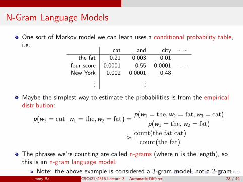
N-Gram Language Models
One sort of Markov model we can learn uses a conditional probability table,i.e.
cat and city · · ·the fat 0.21 0.003 0.01
four score 0.0001 0.55 0.0001 · · ·New York 0.002 0.0001 0.48
......
Maybe the simplest way to estimate the probabilities is from the empiricaldistribution:
p(w3 = cat |w1 = the,w2 = fat) =p(w1 = the,w2 = fat,w3 = cat)
p(w1 = the,w2 = fat)
≈ count(the fat cat)
count(the fat)
The phrases we’re counting are called n-grams (where n is the length), sothis is an n-gram language model.
Note: the above example is considered a 3-gram model, not a 2-grammodel!Jimmy Ba CSC421/2516 Lecture 3: Automatic Differentiation & Distributed Representations28 / 49

N-Gram Language Models
Shakespeare:
Jurafsky and Martin, Speech and Language Processing
Jimmy Ba CSC421/2516 Lecture 3: Automatic Differentiation & Distributed Representations29 / 49

N-Gram Language Models
Wall Street Journal:
Jurafsky and Martin, Speech and Language Processing
Jimmy Ba CSC421/2516 Lecture 3: Automatic Differentiation & Distributed Representations30 / 49

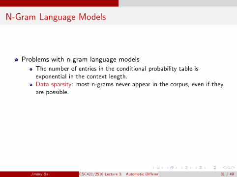
N-Gram Language Models
Problems with n-gram language models
The number of entries in the conditional probability table isexponential in the context length.Data sparsity: most n-grams never appear in the corpus, even if theyare possible.
Traditional ways to deal with data sparsity
Use a short context (but this means the model is less powerful)Smooth the probabilities, e.g. by adding imaginary countsMake predictions using an ensemble of n-gram models with different n
Jimmy Ba CSC421/2516 Lecture 3: Automatic Differentiation & Distributed Representations31 / 49

Distributed Representations
Conditional probability tables are a kind of localist representation: all theinformation about a particular word is stored in one place, i.e. a column of thetable.
But different words are related, so we ought to be able to share informationbetween them. For instance, consider this matrix of word attributes:
academic politics plural person buildingstudents 1 0 1 1 0colleges 1 0 1 0 1legislators 0 1 1 1 0schoolhouse 1 0 0 0 1
And this matrix of how each attribute influences the next word:
bill is are papers built standingacademic − +politics + −plural − +person +building + +
Jimmy Ba CSC421/2516 Lecture 3: Automatic Differentiation & Distributed Representations32 / 49

Imagine these matrices are layers in an MLP. (One-hot representations of words,softmax over next word.)
Here, the information about a given word is distributed throughout therepresentation. We call this a distributed representation.
In general, when we train an MLP with backprop, the hidden units won’t haveintuitive meanings like in this cartoon. But this is a useful intuition pump for whatMLPs can represent.
Jimmy Ba CSC421/2516 Lecture 3: Automatic Differentiation & Distributed Representations33 / 49

Distributed Representations
We would like to be able to share information between related words.E.g., suppose we’ve seen the sentence
The cat got squashed in the garden on Friday.
This should help us predict the words in the sentence
The dog got flattened in the yard on Monday.
An n-gram model can’t generalize this way, but a distributedrepresentation might let us do so.
Jimmy Ba CSC421/2516 Lecture 3: Automatic Differentiation & Distributed Representations34 / 49

Neural Language Model
Predicting the distribution of the next word given the previous K isjust a multiway classification problem.
Inputs: previous K words
Target: next wordLoss: cross-entropy. Recall that this is equivalent to maximumlikelihood:
− log p(s) = − logT∏t=1
p(wt |w1, . . . ,wt−1)
= −T∑t=1
log p(wt |w1, . . . ,wt−1)
= −T∑t=1
V∑v=1
ttv log ytv ,
where tiv is the one-hot encoding for the ith word and yiv is thepredicted probability for the ith word being index v .
Jimmy Ba CSC421/2516 Lecture 3: Automatic Differentiation & Distributed Representations35 / 49

Bengio’s Neural Language Model
Here is a classic neural probabilistic language model, or just neurallanguage model:
Bengio�s neural net for predicting the next word
“softmax” units (one per possible next word)
index of word at t-2 index of word at t-1
learned distributed encoding of word t-2
learned distributed encoding of word t-1
units that learn to predict the output word from features of the input words
table look-up table look-up
skip-layer connections
http://www.jmlr.org/papers/volume3/bengio03a/bengio03a.pdf
Jimmy Ba CSC421/2516 Lecture 3: Automatic Differentiation & Distributed Representations36 / 49

Neural Language Model
If we use a 1-of-K encoding for the words, the first layer can bethought of as a linear layer with tied weights.
The weight matrix basically acts like a lookup table. Each column isthe representation of a word, also called an embedding, featurevector, or encoding.
“Embedding” emphasizes that it’s a location in a high-dimensonalspace; words that are closer together are more semantically similar“Feature vector” emphasizes that it’s a vector that can be used formaking predictions, just like other feature mappigns we’ve looked at(e.g. polynomials)
Jimmy Ba CSC421/2516 Lecture 3: Automatic Differentiation & Distributed Representations37 / 49

Neural Language Model
We can measure the similarity or dissimilarity of two words using
the dot product r>1 r2
Euclidean distance ‖r1 − r2‖If the vectors have unit norm, the two are equivalent:
‖r1 − r2‖2 = (r1 − r2)>(r1 − r2)
= r>1 r1 − 2r>1 r2 + r>2 r2
= 2− 2r>1 r2
In this case, the dot product is called cosine similarity.
Jimmy Ba CSC421/2516 Lecture 3: Automatic Differentiation & Distributed Representations38 / 49

Neural Language Model
This model is very compact: the number of parameters is linear in thecontext size, compared with exponential for n-gram models.
Bengio�s neural net for predicting the next word
“softmax” units (one per possible next word)
index of word at t-2 index of word at t-1
learned distributed encoding of word t-2
learned distributed encoding of word t-1
units that learn to predict the output word from features of the input words
table look-up table look-up
skip-layer connections
Jimmy Ba CSC421/2516 Lecture 3: Automatic Differentiation & Distributed Representations39 / 49

Neural Language Model
What do these word embeddings look like?
It’s hard to visualize an n-dimensional space, but there are algorithmsfor mapping the embeddings to two dimensions.
The following 2-D embeddings are done with an algorithm calledtSNE which tries to make distnaces in the 2-D embedding match theoriginal 30-D distances as closely as possible.
Note: the visualizations are from a slightly different model.
Jimmy Ba CSC421/2516 Lecture 3: Automatic Differentiation & Distributed Representations40 / 49

Neural Language Model
Jimmy Ba CSC421/2516 Lecture 3: Automatic Differentiation & Distributed Representations41 / 49

Neural Language Model
Jimmy Ba CSC421/2516 Lecture 3: Automatic Differentiation & Distributed Representations42 / 49

Neural Language Model
Jimmy Ba CSC421/2516 Lecture 3: Automatic Differentiation & Distributed Representations43 / 49

Neural Language Model
Thinking about high-dimensional embeddings
Most vectors are nearly orthogonal (i.e. dot product is close to 0)Most points are far away from each other“In a 30-dimensional grocery store, anchovies can be next to fish andnext to pizza toppings.” – Geoff Hinton
The 2-D embeddings might be fairly misleading, since they can’tpreserve the distance relationships from a higher-dimensionalembedding. (I.e., unrelated words might be close together in 2-D, butfar apart in 30-D.)
Jimmy Ba CSC421/2516 Lecture 3: Automatic Differentiation & Distributed Representations44 / 49

GloVe
Fitting language models is really hard:
It’s really important to make good predictions about relativeprobabilities of rare words.Computing the predictive distribution requires a large softmax.
Maybe this is overkill if all you want is word representations.
Global Vector (GloVe) embeddings are a simpler and faster approachbased on a matrix factorization similar to principal componentanalysis (PCA).
First fit the distributed word representations using GloVe, then plugthem into a neural net that does some other task (e.g. languagemodeling, translation).
Jimmy Ba CSC421/2516 Lecture 3: Automatic Differentiation & Distributed Representations45 / 49

GloVe
Distributional hypothesis: words with similar distributions have similarmeanings (“judge a word by the company it keeps”)
Consider a co-occurrence matrix X, which counts the number oftimes two words appear nearby (say, less than 5 positions apart)
This is a V × V matrix, where V is the vocabulary size (very large)
Intuition pump: suppose we fit a rank-K approximation X ≈ RR>,where R and R are V × K matrices.
Each row ri of R is the K -dimensional representation of a wordEach entry is approximated as xij ≈ r>i rjHence, more similar words are more likely to co-occurMinimizing the squared Frobenius norm‖X− RR>‖2
F =∑
i,j(xij − r>i rj)2 is basically PCA.
Jimmy Ba CSC421/2516 Lecture 3: Automatic Differentiation & Distributed Representations46 / 49

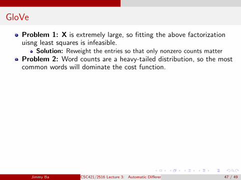
GloVe
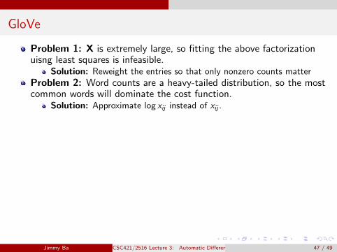
Problem 1: X is extremely large, so fitting the above factorizationuisng least squares is infeasible.
Solution: Reweight the entries so that only nonzero counts matterProblem 2: Word counts are a heavy-tailed distribution, so the mostcommon words will dominate the cost function.
Solution: Approximate log xij instead of xij .
Global Vector (GloVe) embedding cost function:
J (R) =∑i,j
f (xij)(r>i rj + bi + bj − log xij)2
f (xij) =
{( xij100
)3/4if xij < 100
1 if xij ≥ 100
bi and bj are bias parameters.
We can avoid computing log 0 since f (0) = 0.
We only need to consider the nonzero entries of X. This gives a bigcomputational savings since X is extremely sparse!
Jimmy Ba CSC421/2516 Lecture 3: Automatic Differentiation & Distributed Representations47 / 49

GloVe
Problem 1: X is extremely large, so fitting the above factorizationuisng least squares is infeasible.
Solution: Reweight the entries so that only nonzero counts matter
Problem 2: Word counts are a heavy-tailed distribution, so the mostcommon words will dominate the cost function.
Solution: Approximate log xij instead of xij .
Global Vector (GloVe) embedding cost function:
J (R) =∑i,j
f (xij)(r>i rj + bi + bj − log xij)2
f (xij) =
{( xij100
)3/4if xij < 100
1 if xij ≥ 100
bi and bj are bias parameters.
We can avoid computing log 0 since f (0) = 0.
We only need to consider the nonzero entries of X. This gives a bigcomputational savings since X is extremely sparse!
Jimmy Ba CSC421/2516 Lecture 3: Automatic Differentiation & Distributed Representations47 / 49
GloVe
Problem 1: X is extremely large, so fitting the above factorizationuisng least squares is infeasible.
Solution: Reweight the entries so that only nonzero counts matterProblem 2: Word counts are a heavy-tailed distribution, so the mostcommon words will dominate the cost function.
Solution: Approximate log xij instead of xij .
Global Vector (GloVe) embedding cost function:
J (R) =∑i,j
f (xij)(r>i rj + bi + bj − log xij)2
f (xij) =
{( xij100
)3/4if xij < 100
1 if xij ≥ 100
bi and bj are bias parameters.
We can avoid computing log 0 since f (0) = 0.
We only need to consider the nonzero entries of X. This gives a bigcomputational savings since X is extremely sparse!
Jimmy Ba CSC421/2516 Lecture 3: Automatic Differentiation & Distributed Representations47 / 49

Word Analogies
Here’s a linear projection of word representations for cities and capitals into2 dimensions.
The mapping city → capital corresponds roughly to a single direction in thevector space:
Note: this figure actually comes from skip-grams, a predecessor to GloVe.
Jimmy Ba CSC421/2516 Lecture 3: Automatic Differentiation & Distributed Representations48 / 49
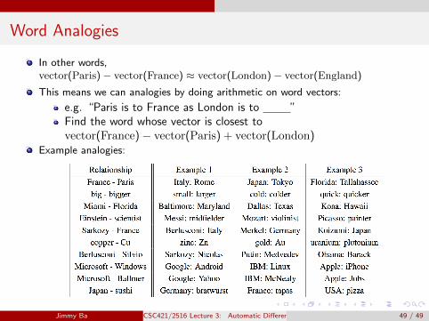
Word Analogies
In other words,vector(Paris)− vector(France) ≈ vector(London)− vector(England)
This means we can analogies by doing arithmetic on word vectors:
e.g. “Paris is to France as London is to ”Find the word whose vector is closest tovector(France)− vector(Paris) + vector(London)
Example analogies:
Jimmy Ba CSC421/2516 Lecture 3: Automatic Differentiation & Distributed Representations49 / 49


![CSC421/2516 Lecture 17: Variational Autoencodersrgrosse/courses/csc421_2019/slides/lec17.pdf · The reconstruction term E q[log p(xjz)] = 1 2 ... Roger Grosse and Jimmy Ba CSC421/2516](https://static.fdocuments.net/doc/165x107/5f555c4b451834262b22de03/csc4212516-lecture-17-variational-rgrossecoursescsc4212019slideslec17pdf.jpg)