CSC2535: Computation in Neural Networks

Lecture 12: Non-linear dimensionality reduction

Geoffrey Hinton

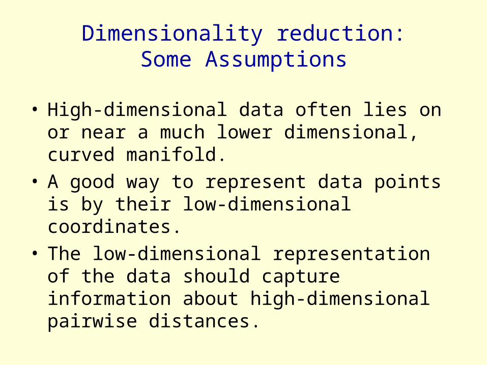
Dimensionality reduction: Some Assumptions

• High-dimensional data often lies on or near a much lower dimensional, curved manifold.

• A good way to represent data points is by their low-dimensional coordinates.

• The low-dimensional representation of the data should capture information about high-dimensional pairwise distances.

Dimensionality reduction methods

• Global methods assume that all pairwise distances are of equal importance.– Choose the low-D pairwise distances to fit the

high-D ones (using magnitude or rank order).

• Local methods assume that only local distances are reliable in high-D.– Put more weight on getting local distances

right.

Linear methods of reducing dimensionality• PCA finds the directions that have the most variance.

– By representing where each datapoint is along these axes, we minimize the squared reconstruction error.

– Linear autoencoders are equivalent to PCA

• Multi-Dimensional Scaling arranges the low-dimensional points so as to minimize the discrepancy between the pairwise distances in the original space and the pairwise distances in the low-D space.

• MDS is equivalent to PCA (if we normalize the data right)

2|||||||| ij

jijiCost yyxx

high-D distance

low-D distance

• Multi-Dimensional Scaling can be made non-linear by putting more importance on the small distances. An extreme version is the Sammon mapping:

• Non-linear MDS is also slow to optimize and also gets stuck in different local optima each time.

Other non-linear methods of reducing dimensionality

2

||||

||||||||

ji

jiji

ji

Costxx

yyxx

high-D distance

low-D distance

Linear methods cannot interpolate properly between the leftmost and rightmost images in each row.

This is because the interpolated images are NOT averages of the images at the two ends.

The method shown here does not interpolate properly either because it can only use examples from the training set. It cannot create new images.

IsoMap: Local MDS without local optima

• Instead of only modeling local distances, we can try to measure the distances along the manifold and then model these intrinsic distances.– The main problem is to find a

robust way of measuring distances along the manifold.

– If we can measure manifold distances, the global optimisation is easy: It’s just global MDS (i.e. PCA)

2-D

1-D

If we measure distances along the manifold, d(1,6) > d(1,4)

1

46

How Isomap measures intrinsic distances

• Connect each datapoint to its K nearest neighbors in the high-dimensional space.

• Put the true Euclidean distance on each of these links.

• Then approximate the manifold distance between any pair of points as the shortest path in this graph.

A

B

Using Isomap to discover the intrinsic manifold in a set of face images

A probabilistic version of local MDS

• It is more important to get local distances right than non-local ones, but getting infinitessimal distances right is not infinitely important.– All the small distances are about equally

important to model correctly.– Stochastic neighbor embedding has a

probabilistic way of deciding if a pairwise distance is “local”.

Stochastic Neighbor Embedding:A probabilistic local method

• Each point in high-D has a probability of picking each other point as its neighbor.

• The distribution over

neighbors is based on the high-D pairwise distances.

High-D Space

i

jk

222

222

iikd

k

iijd

ij

e

ep

Throwing away the raw data

• The probabilities that each points picks other points as its neighbor contains all of the information we are going to use for finding the manifold.– Once we have the probabilities we do not need

to do any more computations in the high-dimensional space.

– The input could be “dissimilarities” between pairs of datapoints instead of the locations of individual datapoints in a high-dimensional space.

ijp

Evaluating an arrangement of the data in a low-dimensional space

• Give each datapoint a location in the low- dimensional space.– Evaluate this

representation by seeing how well the low-D probabilities model the high-D ones.

Low-D Space

i

j

k

2

2

ikd

k

ijd

ije

eq

The cost function for a low-dimensional representation

• For points where pij is large and qij is small we lose a lot.– Nearby points in high-D really want to be nearby in

low-D• For points where qij is large and pij is small we lose a

little because we waste some of the probability mass in the Qi distribution.– Widely separated points in high-D have a mild

preference for being widely separated in low-D.

ij

ij

i jij

ii q

ppQPKLCost i log)||(

The forces acting on the low-dimensional points

• Points are pulled towards each other if the p’s are bigger than the q’s and repelled if the q’s are bigger than the p’s

)()( jijiijijij

ji

qpqpCost

yyy

i

j

Unsupervised SNE embedding of the digits 0-4. Not all the data is displayed

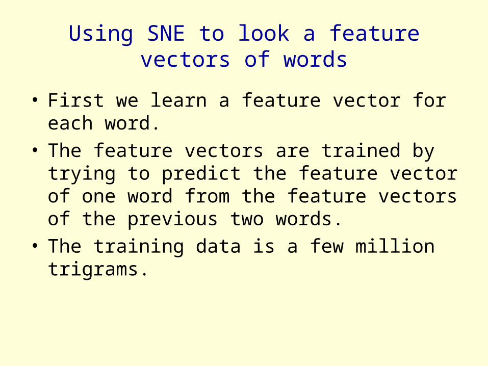
Using SNE to look a feature vectors of words

• First we learn a feature vector for each word.• The feature vectors are trained by trying to

predict the feature vector of one word from the feature vectors of the previous two words.

• The training data is a few million trigrams.

A net for learning what words mean? (Andriy Mnih)

• The net is given two words and asked to predict the next word.

• It learns to represent each word as a vector of 100 real-valued features.

1000 binary neurons

100 reals

“open” “the”

100 reals 100 reals

?

A table that converts each word to its feature vector can be learned at the same time as learning the conditional Boltzmann machine

Symmetric SNE

• In general, the probability of I picking j is not equal to the probability of j picking i.

• But we could symmetrize to get probabilities of picking pairs of datapoints.

Computing affinities between datapoints

• Each high dimensional point, i, has a conditional probability of picking each other point, j, as its neighbor.

• The conditional distribution

over neighbors is based on the high-dimensional pairwise distances.

High-D Space

i

jk

222

222

|iikd

k

iijd

ij

e

ep

probability of picking j given that you start at i

Turning conditional probabilities into pairwise probabilities

To get a symmetric affinity between i and j we sum the two conditional probabilities and divide by the number of points (points are not allowed to choose themselves).

This ensures that all the pairwise affinities sum to 1 so they can be treated as probabilities.

11 1

n

iij

n

ijjiij pp

n

ppp jiijij

|| joint probability of

picking the pair i,j

Evaluating an arrangement of the data in a low-dimensional space

• Give each data-point a location in the low- dimensional space.– Define low-dimensional

probabilities symmetrically.– Evaluate the

representation by seeing how well the low-D probabilities model the high-D affinities.

Low-D Space

i

j

k

2

2

kld

lk

ijd

ije

eq

The cost function for a low-dimensional representation

• For points where pij is large and qij is small we lose a lot.– Nearby points in high-D really want to be nearby in

low-D• For points where qij is large and pij is small we lose a

little because we waste some of the probability mass in the Q distribution.– Widely separated points in high-D have a mild

preference for not being too close in low-D.– But it doesn’t cost much to make the manifold bend

back on itself.

ji ij

ijij q

ppQPKLCost log|)||(

The forces acting on the low-dimensional points

• Points are pulled towards each other if the p’s are bigger than the q’s and repelled if the q’s are bigger than the p’s– Its equivalent to having

springs whose stiffnesses are set dynamically.

)()(2)||(

ijijjj

ii

qpQPKL

yyy

i

j

extension stiffness

Evaluating the codes found by a deep autoencoder

• Use 3000 images of handwritten digits from the USPS training set.– Each image is 16x16

and fairly binary. • Use a highly non-linear

autoencoder – Use logistic output units

and linear code units. 200 logistic units

100 logistic units

20 linear code units

data

reconstruction

Does code space capture the structure of the data?

• We would like the code space to model the underlying structure of the data.– Digits in the same class should get closer together in

code space.– Digits of different classes should get further apart.

• We can use k nearest neighbors to see if this happens.– Hold out each image in turn and try to label it by using

the labels of its k nearest neighbors.

A potential problem

• PCA is not powerful enough to really mangle the data.

• Highly non-linear auto-encoders can fracture a manifold into many different domains.– This can lead to very

different codes for nearby data-points.

AB

C

A B C

AB

C A C

B

How to fix it

• We use a regularizer that makes it costly to fracture the manifold.– There are many possible regularizers.

• Stochastic neighbor embedding can be used as a regularizer.– Its like putting springs between the codes to

prevent the codes for similar datapoints from being too far apart.

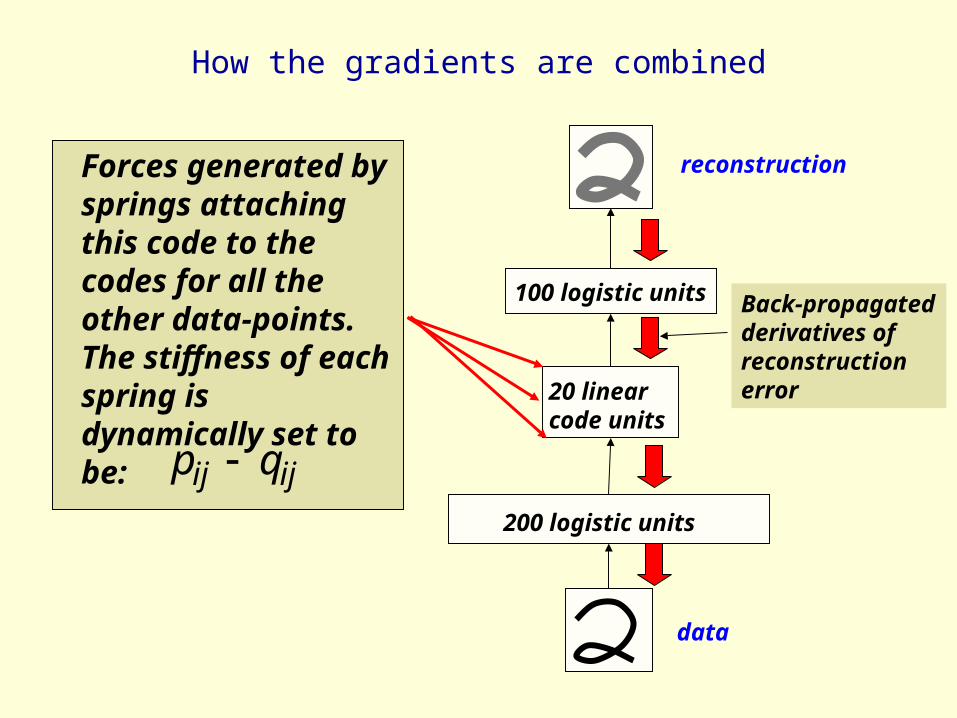
How the gradients are combined

200 logistic units

100 logistic units

20 linear code units

data

reconstructionForces generated by springs attaching this code to the codes for all the other data-points. The stiffness of each spring is dynamically set to be: ijij qp

Back-propagated derivatives of reconstruction error

How well does it work?(Hinton, Min, Salakhutdinov)

• The hold-one-out KNN error of an autoencoder falls if we combine it with SNE.– SNE makes the search easier for a deep

autoencoder.– The strength of the regularizer must be chosen

sensibly.– The SNE regularizer alone gives higher hold-one-out

KNN errors than a well trained autoencoder• Can we visualize the codes that are produced using the

regularizer?

Using SNE for visualization

• To get an idea of the similarities between codes, we can use SNE to map the 20-D codes down to 2-D.– The combination of the generative model of

the auto-encoder and the manifold preserving regularizer causes the codes for different classes of digit to be quite well separated.