CSC 778 - Optical Networking Rudra Dutta, Fall 2007 NP-Completeness, Optimization, in Network...

CSC 778 - Optical NetworkingCSC 778 - Optical NetworkingRudra Dutta, Fall 2007Rudra Dutta, Fall 2007

NP-Completeness, Optimization, in Network Design

Copyright Rudra Dutta, NCSU, Fall, 2007 2

Complexity and OptimizationComplexity and Optimization Most “problems” are NOT “solvable”

– Others are merely hard to solve– This includes many practically interesting problems

Sometimes solutions are not just costly, but...– Difficult or impossible to express

Optimization techniques allow modeling such problems– Sometimes provide “good” if not “perfect” solutions

Bottom-line: part of the language of complex network design, must understand

Complexity Theory,Complexity Theory,NP-CompletenessNP-Completeness


AlgorithmsAlgorithms Information representation by bits Algorithms as manipulators of bits Abstract manipulations of abstract data types

– Not specific to machine architecture etc.


Asymptotic ComplexityAsymptotic Complexity Complexity - number of elemental steps

required– What is a step?– Worst case, average case?

Naturally, problem instances of bigger “size” can reasonably take more steps

Asymptotic - beyond a certain “size”f,g: N N

f is O(g) iff N,c: f(n) c g(n) n Ng is (f)

f is (g) iff f is O(g) and (g)


LanguagesLanguages Alphabet - a finite set of symbols () String - finite ordered list of symbols from

– The empty string is denoted by Universe of strings *

– All strings of length k - k

Concatenation, suffix, prefix, substring Language - a subset of * Characteristic function cL

Examples on = {0,1}– L = {00,01,10,11} = 2 – L = {x ends with a single 0 after one or more 1’s}


Infinite Sets and ComputabilityInfinite Sets and Computability Function, domain, co-domain, range Surjective (onto)

– Range = co-domain Injective (one-to-one)

– Distinct elements mapped to distinct elements Bijective: both Bijection allows comparison of infinite set sizes

– |N| = |E| = |O| = 0 , countable infinity– Q = N x N, 0 . 0 = 0 – Diagonalization argument : R is not countable– 2N is not countable - most functions not computable


AutomataAutomata Finite Automata or FSM

– States, transition function– FSM’s as language acceptors

Determinism– NDFA: accept if an accepting sequence exists– Magic– DFA’s in parallel (not inherently different from DFA)

1

1 000,1

0,10,1

0,1

0,1 0

11

0


Computational ModelsComputational Models A language (or function) is a problem

– Program computes desirable quantity for each instance of a problem - decision or optimization

Regular expressions and regular languages– Shown to be equivalent to finite automata

The Halting Problem– A diagonalization argument on programs– Assume such a program exists– Make another which stops only if it returns “yes”

Universal models of computation– Several now known, (polynomial) equivalent


Turing MachinesTuring Machines Turing machine is quite convenient

– Concept of “steps” and “space” are obvious– Difference in scale with practical computers

Reads problem on tape, ends with solution– Non-determinism does not increase power– Multiple tapes do not increase power

Acceptors and enumerators

Finite-state control


ComputabilityComputability Primitive Recursive functions

– Zero, Succ, Pick– Build other functions by:

SubstitutionPrimitive recursion: f(0) = x, f(i + 1) = h(i, f(i))

PR functions are computable, but computable functions that are not PR exist– Diagonalization

Partial Recursive functions– Not defined for all input - avoid diagonalization– µ-recursion or minimization: find minimum (extra)

argument that makes another function return zero


Function ClassesFunction Classes

All partial functions

total not totalpartial recursive

primitiverecursive


Further on ComputabilityFurther on Computability Recursive and R.E. sets Rice’s Theorem Reductions, classes of reduction Hardness, easiness, completeness


Classes and ReductionsClasses and Reductions Some problems are equivalent to others Others are “at least as difficult as” Concept of reduction

– More explanatory names: “equivalence” or “transformability”

Different kinds of reduction– Generic versus specific– Turing versus many-to-one

Reductions allow equivalence classes to be built– But finding first complete problem (generic) could be

difficult


Equivalence ClassesEquivalence Classes


Cook’s TheoremCook’s Theorem Satisfiability is NP-Complete

– A collection of Boolean clauses– Problem: Decide whether truth assignment satisfying

all the clauses exists

Given an instance of a decision problem in NP, an instance of Satisfiability can be produced in polynomial time, which is satisfiable iff the original instance is a “yes” instance


Many-to-One ReductionsMany-to-One Reductions First show problem at hand is in NP Pick a known NPC problem to reduce from

– All instances of the problem must be amenable to reduction

– If not, danger of picking tractable subset Define a function to transform instance into

instance of target– Must be polynomial procedure– Need not reach all instances of target– Hence many-to-one, not one-to-one or onto

Special case: restriction– Of problem space, not solution method


Decision and OptimizationDecision and Optimization Most problems can be stated in either of two

versions Generally interchangable

– Proof of computational complexity class with one is often taken as proof for another

– Complexity proofs attempted for decision versions

Decision - quantified yes-no question– “Can you finish your shopping within x dollars?”

Optimization - best-of-class question– “How few dollars can you finish your shopping

within?”


Well Known NPC ProblemsWell Known NPC Problems Three-satisfiability

– Each clause has exactly three literals– 1in3Sat– NAE3Sat

MaxCut Partition Exact Cover by 3-sets Chromatic number Knapsack Bin-packing


An ExampleAn Example Knapsack: Given a set of elements, a positive integer

size and value for each, a positive integer size upper bound and value lower bound, does a subset meeting the bounds exist?

Partition: Given a set of elements, each with a positive integer size such that the sum of all sizes is an even number, can the set by partitioned into two subsets such that the sum of elements in each subset is equal?

Restriction: In Knapsack, allow only instances where the sum of all sizes is a multiple of 2, size equals value for each element, and bounds are each equal to half the sum of sizes


ApproximationsApproximations Practically, very close may be as good as there “Close” is defined as fraction of or difference

from the optimal objective value– Must be constant

An approximation to an NPC problem which is in P is quite valuable

May be possible to customize the algorithm to obtain any desired approximation ratio– Polynomial Time Approximation Scheme

However, many problems are NP-approximable


Networking ContextNetworking Context Many network design problems are complex It is important to know whether optimal solutions

may be tractably attempted If not, approximations/heuristics may be

attempted NPC reduction method may provide an insight

into profitable heuristic methods


Flow Maximization Flow Maximization Concept of “commodity flow” Network modeled as a digraph with capacitated links Designated “source” nodes produce commodity Designated “sink” nodes consume Problem: to maximize commodity flow (or to decide

whether a given flow can be obtained)


Flow Augmentation AlgorithmFlow Augmentation Algorithm Max-flow Min-cut theorem

– The maximal amount of flow is equal to the capacity of a minimal cut

– Formalization of the concept of bottleneck Equivalent: no augmenting path can be found in

the residual network Residual - update capacity by subtracting flow

– May create positive capacity links out of zero capacity links (reverse flow)

Augmenting path - path with positive capacity Iterate to get maximum flow


Minimum Cost 1-Commodity FlowMinimum Cost 1-Commodity Flow More practical problem

– Every link has cost as well as capacity– Posed with integer cost, supply/demand, capacity– Total supply equals total demand

Question: can a given flow to/from s-/d-nodes be achieved within a given cost bound?

– Feasibility can be checked using max-flow approach Polynomial problem

– Several known polynomial time algorithms– Capacity scaling algorithm, e.g.– Simpler version: successive shortest path

algorithm Not strictly polynomial

– Refer to excerpt from Ahuja, Magnanti, Orlin


Successive Shortest PathSuccessive Shortest Path Mass balance: amounts of incoming of outgoing

flow balance to total source or sink requirement of a node (zero if it is neither source nor sink)

Pseudoflow: flow function which obeys non-negativity and capacity, but not mass balance– Imbalance of a node: difference in flow in and out,

corrected by supply/demand Potential: a value maintained for each node Keep a pseudoflow and a potential vector, both

initially zero Initially all imbalances are equal to supply


Successive Shortest PathSuccessive Shortest Path Choose a node k with excess and a node l with

deficit Calculate shortest path distances from k to all

other nodes– Use edge costs corrected by node potential

differences as costs– Update node potentials, reducing by shortest path

cost from k Choose a particular path from k to l

– Augment the pseudoflow as much as possible, not exceeding capacity of any link or imbalance of k or l

Repeat until no imbalance exists


Multi-Commodity FlowMulti-Commodity Flow Capacitated, cost-weighted digraph, as before Now there are distinct “commodities”

– Producers and consumers for each commodity must be matched, cannot be interchanged

In particular, every node may generate a unique commodity for every other node

– N x (N-1) distinct commodities

Question: can a given set of commodity flows to/from s-/d-nodes be achieved within a given cost bound?

Significantly more difficult In fact, NP-complete Optimization version often of practical interest

OptimizationOptimization


OptimizationOptimization Another name for minimization or maximization Usually used when quantity (function) is

– Built of complex combinations of variables– Does not vary smoothly like “normal” functions

Conceptual difficulty in describing the problem– Basic entities may be many, of different kinds– Consider the multi-commodity flow problem– Or the simpler version we attempted in class– Contrast with, say, Traveling Salesman Problem


ElementsElements Parameters

– Given input values, constant for a given instance– The list of weights and values in Knapsack, e.g.

Variables– Required output values in solution– List of “yes/no” answers for each object

Constraints– Reflection of characteristics of real-life problem– “Knapsack cannot hold more than 50 lb and remain intact”

Objective– Definition of quantity to be maximized or minimized– Total value of objects tagged “yes” in answer


Static OptimizationStatic Optimization Distinct from dynamic or stochastic optimization Mathematical programming problems

– Minimize F(x)– Subject to x S

x is the variable vector S represents constraints (with parameters) F() is the objective function S is a (feasible) solution set or optimization space If S is empty the problem is infeasible We are often interested in the specific class of ((Mixed)

Integer ) Linear Programming problems


Feasible RegionFeasible Region Much of the ease or

difficulty of a problem lies in the shape of the feasible region

If some regular traversal of the solution space exists for which objective function exhibits simple increase or decrease, easy to solve

Difficulty arises when no such traversal exists or is apparent


ConvexityConvexity S is convex if for all points x, y S, the whole segment

joining x and y belongs to S – {x + (1 - ) y : 0 1} S

A function f on S is a convex function if x, y S, [0, 1]– f (x + (1 - ) y) f (x) + (1 - ) f (y)

Concavity, strictly convex (concave) If F and S are both convex, such problems have nice

properties and are easier to solve Discrete analogue to convexity Pareto optimal - for multiple objectives Fi, a solution

such that no other exists– At least as good for all, and better for at least one objective


Gradient and DifferentiabilityGradient and Differentiability Gradient - generalization of derivative

– Vector of partial (directional) derivatives–

If a point is a local minimum, gradient is zero at that point– For convex functions, an interior point which is a local

minimum is also a global minimum

Hessian - square matrix of second order partial derivatives– If Hessian is PSD at an interior gradient zero point,

that point is locally optimal


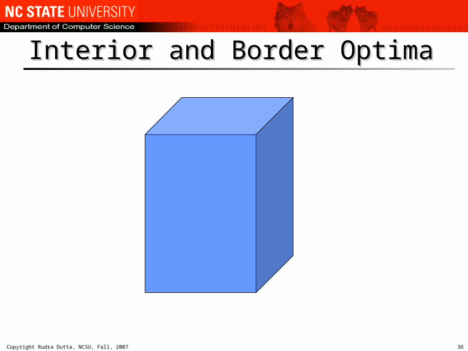
Interior and Border OptimaInterior and Border Optima


Karush-Kuhn-Tucker ConditionsKarush-Kuhn-Tucker Conditions Often local minima are attained at border points, not

interior points– Must be characterized by other means

Let S be defined by (all hi and gj differentiable):

Then multipliers (unconstrained sign) and (non-negative) exist such that:


Further ConceptsFurther Concepts Perturbation - sensitivity Gradient descent - numerical methods Duality Subgradient Maximization Relaxation


RelaxationRelaxation Removing some constraints - relaxing

– Makes the solution space larger– But may make the problem “easier”– Provides bound on optimal objective of original

Removing integer constraints– LP is possible to solve, so beneficial if linear system

Lagrangian relaxation– Solving the dual of the given problem– Convert one or more or all the constraints into “violation costs”

in objective– For given multipliers, often easy to solve– Now optimize new cost get values for multipliers– Results regarding the “duality gap”, “complementary slack”


Duality and LagrangianDuality and Lagrangian

Primal: Lagrangian Function:

Dual Function:

Dual Problem:


Example: KnapsackExample: Knapsack Consider the knapsack instance

– {(8,16), (9,20), (5,12), (4,10)} (value, weight)– Weight bound 42, optimization version

Optimization formulation:– Maximize 8x1 + 9x2 + 5x3 + 4x4

– S.t. 16x1 + 20x2 + 12x3 + 10x4 ≤ 42– xi {0,1} i

Not obvious (in general NPC, as we know) But remove the inequality constraint

– Now trivial, set all xi = 1– Clearly a bound, but not a very good one– Next?


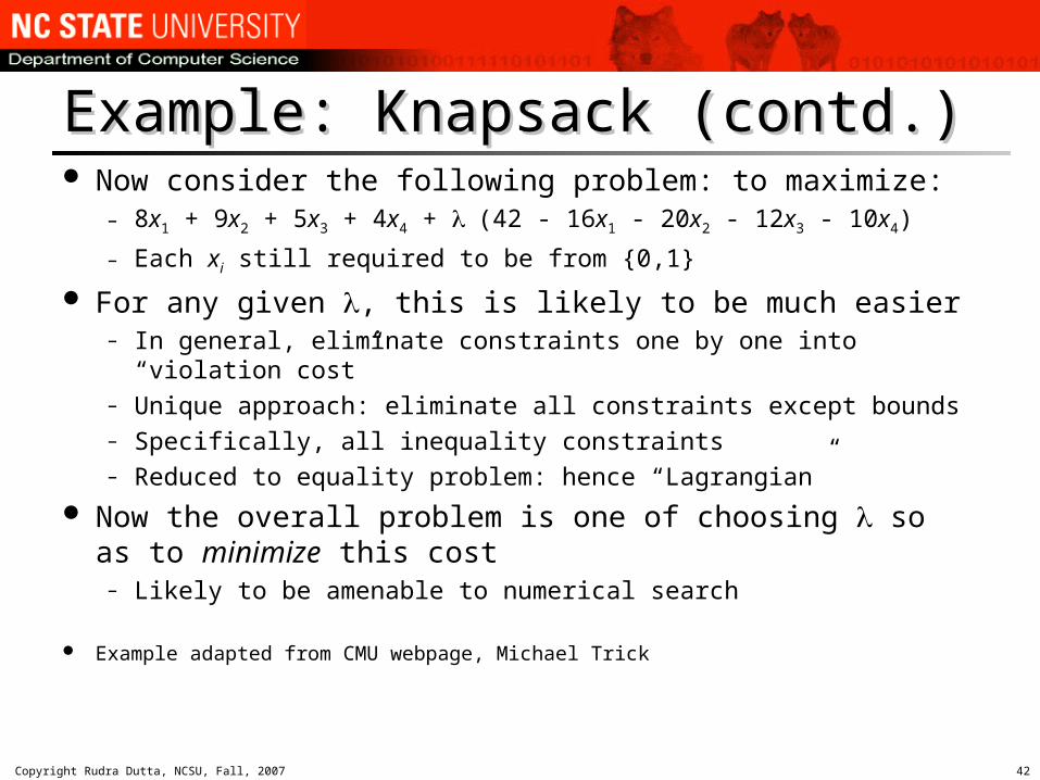
Example: Knapsack (contd.)Example: Knapsack (contd.) Now consider the following problem: to maximize:

– 8x1 + 9x2 + 5x3 + 4x4 + (42 - 16x1 - 20x2 - 12x3 - 10x4)

– Each xi still required to be from {0,1}

For any given , this is likely to be much easier– In general, eliminate constraints one by one into “violation cost”– Unique approach: eliminate all constraints except bounds– Specifically, all inequality constraints– Reduced to equality problem: hence “Lagrangian”

Now the overall problem is one of choosing so as to minimize this cost

– Likely to be amenable to numerical search

Example adapted from CMU webpage, Michael Trick


(Integer) Linear Programs(Integer) Linear Programs Linear - all constraints can be posed as only linear combinations of

variables– For long complexity was open - thought NPI

Comparatively recently resolved to be polynomial– Simplex is exponential but usually runs faster

If the polyhedron of feasible region has extreme points, and an optimal exists, an extreme optimal exists

Strictly polynomial methods (elliptical, interior points) exist Integer - all (pure) or some (mixed) variables are constrained to be

integers– Jump in practical difficulty level - NPC– Branch-and-bound, dynamic programing, …

Relaxation of integer constraints is an obvious way to solve practically

– Need to round off solutions– But if integer constraints are binary, not a good method– In general binary problems are harder and “best” formulations are not

easy to characterize


Network ContextNetwork Context Many networking problems are linear programs

– Commodity flow problems– Objective function sometimes poses problems– Integer constraints often appear

We are interested not only in optimal value, but also actual solution

Practically, solving ILP is not a good approach However, domain specific knowledge may allow

specific relaxation or other approach


Multi-Commodity Flow FormulationMulti-Commodity Flow Formulation Parameters

– n : number of nodes– A : set of all links (i, j) – uij : bitrate of link– cij : cost per bit on link– bkl : traffic demand from node k to node l

Variables– xkl

ij : traffic from k to l using link from i to j Goal: minimize total cost

Source: Bertsimas and Tsitsilkis

j

l

i

k


Multi-Commodity Flow FormulationMulti-Commodity Flow Formulation

i


Node-Link and Link-PathNode-Link and Link-Path Two ways of formulating the same thing Node-link - nodes, links are entities of interest

– Focus on traffic demand to and from nodes, on links – Bridging variable - demand between nodes on links– Like previous example

Link-path - links, paths are entities of interest– Demand is still between nodes– For each given demand node pair, list all paths– Assign variable to path traffic flow (implicitly identifies

demand)– For each link, sum up path flow variables, and

constrain with capacities


Programming AssignmentProgramming Assignment Implement the flow augmentation algorithm for

single-commodity flow maximization Implement the successive shortest path

algorithm for minimum-cost commodity flow Realize the ILP formulation for multi-commodity

flow in CPLEX

CSC 778 - Optical Networking Rudra Dutta, Fall 2007 NP-Completeness, Optimization, in Network...

Documents

Transcript of CSC 778 - Optical Networking Rudra Dutta, Fall 2007 NP-Completeness, Optimization, in Network...