CS6301 Programming and Data Structures...

CS6301 Programming and Data Structures II Unit 5

CS6301 Programming and Data Structures II

Unit -5

REPRESENTATION OF GRAPHS

Graph and its representations

Graph is a data structure that consists of following two components:

1. A finite set of vertices also called as nodes.

2. A finite set of ordered pair of the form (u, v) called as edge. The pair is ordered because (u, v)

is not same as (v, u) in case of directed graph(di-graph). The pair of form (u, v) indicates that

there is an edge from vertex u to vertex v. The edges may contain weight/value/cost.

Graphs are used to represent many real life applications: Graphs are used to represent networks.

The networks may include paths in a city or telephone network or circuit network. Graphs are

also used in social networks like linkedIn, facebook. For example, in facebook, each person is

represented with a vertex(or node). Each node is a structure and contains information like person

id, name, gender and locale. This can be easily viewed by

http://graph.facebook.com/barnwal.aashish where barnwal.aashish is the profile name. See this

for more applications of graph.

Following is an example undirected graph with 5 vertices.

Following two are the most commonly used representations of graph.

www.studentsfocus.com



1. Adjacency Matrix

2. Adjacency List

There are other representations also like, Incidence Matrix and Incidence List. The choice of the

graph representation is situation specific. It totally depends on the type of operations to be

performed and ease of use.

Adjacency Matrix:

Adjacency Matrix is a 2D array of size V x V where V is the number of vertices in a graph. Let

the 2D array be adj[][], a slot adj[i][j] = 1 indicates that there is an edge from vertex i to vertex j.

Adjacency matrix for undirected graph is always symmetric. Adjacency Matrix is also used to

represent weighted graphs. If adj[i][j] = w, then there is an edge from vertex i to vertex j with

weight w.

The adjacency matrix for the above example graph is:

Adjacency Matrix Representation of the above graph

Pros: Representation is easier to implement and follow. Removing an edge takes O(1) time.

Queries like whether there is an edge from vertex ‘u’ to vertex ‘v’ are efficient and can be done

O(1).

Cons: Consumes more space O(V^2). Even if the graph is sparse(contains less number of edges),

it consumes the same space. Adding a vertex is O(V^2) time.

Adjacency List:




An array of linked lists is used. Size of the array is equal to number of vertices. Let the array be

array[]. An entry array[i] represents the linked list of vertices adjacent to the ith vertex. This

representation can also be used to represent a weighted graph. The weights of edges can be

stored in nodes of linked lists. Following is adjacency list representation of the above graph.

Adjacency List Representation of the above Graph

BREADTH-FIRST SEARCH

In graph theory, breadth-first search (BFS) is a graph search algorithm that begins at the root

node and explores all the neighboring nodes. Then for each of those nearest nodes, it explores

their unexplored neighbor nodes, and so on, until it finds the goal.

x If the element sought is found in this node, quit the search and return a result.

x Otherwise enqueue any successors (the direct child nodes) that have not yet been

discovered.

1 procedure BFS(Graph,source):

2 create a queue Q

3 enqueue source onto Q

4 mark source

5 while Q is not empty:

6 dequeue an item from Q into v

7 for each edge e incident on v in Graph:

8 let w be the other end of e



Sri Vidya College of Engineering & Technology, Virudhunagar Course Material (Lecture Note)


9 if w is not marked:

10 mark w

11 enqueue w onto Q

DEPTH-FIRST SEARCH (DFS)

Depth-first search, or DFS, is a way to traverse the graph. Initially it allows visiting vertices of

the graph only, but there are hundreds of algorithms for graphs, which are based on DFS.

Therefore, understanding the principles of depth-first search is quite important to move ahead

into the graph theory. The principle of the algorithm is quite simple: to go forward (in depth)

while there is such possibility, otherwise to backtrack.

Algorithm

In DFS, each vertex has three possible colors representing its state:

white: vertex is unvisited;

gray: vertex is in progress;

black: DFS has finished processing the vertex.

NB. For most algorithms boolean classification unvisited / visited is quite enough, but we

show general case here.

Initially all vertices are white (unvisited). DFS starts in arbitrary vertex and runs as follows:

1. Mark vertex u as gray (visited).

2. For each edge (u, v), where u is white, run depth-first search for u recursively.

3. Mark vertex u as black and backtrack to the parent.

Example. Traverse a graph shown below, using DFS. Start from a vertex with number 1.




Source graph.

Mark a vertex 1 as gray.

There is an edge (1, 4) and a vertex 4 is

unvisited. Go there.




Mark the vertex 4 as gray.

There is an edge (4, 2) and vertex a 2 is







There are no ways to go from the vertex

3. Mark it as black and backtrack to the

vertex 5.

There is an edge (5, 4), but the vertex 4 is

gray.




There are no ways to go from the vertex

5. Mark it as black and backtrack to the

vertex 2.

There are no more edges, adjacent to

vertex 2. Mark it as black and backtrack

to the vertex 4.

There is an edge (4, 5), but the vertex 5 is

black.




There are no more edges, adjacent to the

vertex 4. Mark it as black and backtrack

to the vertex 1.

There are no more edges, adjacent to the

vertex 1. Mark it as black. DFS is over.

As you can see from the example, DFS doesn't go through all edges. The vertices and edges,

which depth-first search has visited is a tree. This tree contains all vertices of the graph (if it

is connected) and is called graph spanning tree. This tree exactly corresponds to the recursive

calls of DFS.If a graph is disconnected, DFS won't visit all of its vertices.

TOPOLOGICAL SORT

In computer science, a topological sort (sometimes abbreviated topsort or toposort) or

topological ordering of a directed graph is a linear ordering of its vertices such that for every

directed edge uv from vertex u to vertex v, u comes before v in the ordering. For instance, the

vertices of the graph may represent tasks to be performed, and the edges may represent

constraints that one task must be performed before another; in this application, a topological




ordering is just a valid sequence for the tasks. A topological ordering is possible if and only if the

graph has no directed cycles, that is, if it is a directed acyclic graph (DAG). Any DAG has at

least one topological ordering, and algorithms are known for constructing a topological ordering

of any DAG in linear time.

The canonical application of topological sorting (topological order) is in scheduling a sequence

of jobs or tasks based on their dependencies; topological sorting algorithms were first studied in

the early 1960s in the context of the PERT technique for scheduling in project management

(Jarnagin 1960). The jobs are represented by vertices, and there is an edge from x to y if job x

must be completed before job y can be started (for example, when washing clothes, the washing

machine must finish before we put the clothes to dry). Then, a topological sort gives an order in

which to perform the jobs.

In computer science, applications of this type arise in instruction scheduling, ordering of formula

cell evaluation when recomputing formula values in spreadsheets, logic synthesis, determining

the order of compilation tasks to perform in makefiles, data serialization, and resolving symbol

dependencies in linkers. It is also used to decide in which order to load tables with foreign keys

in databases.

The graph shown to the left has many valid topological sorts, including:

7, 5, 3, 11, 8, 2, 9, 10 (visual left-to-right, top-to-bottom)

3, 5, 7, 8, 11, 2, 9, 10 (smallest-numbered available vertex first)




5, 7, 3, 8, 11, 10, 9, 2 (fewest edges first)

7, 5, 11, 3, 10, 8, 9, 2 (largest-numbered available vertex first)

7, 5, 11, 2, 3, 8, 9, 10 (attempting top-to-bottom, left-to-right)

3, 7, 8, 5, 11, 10, 2, 9 (arbitrary)

Algorithms

The usual algorithms for topological sorting have running time linear in the number of nodes

plus the number of edges, asymptotically, O(\left|{V}\right| + \left|{E}\right|).

One of these algorithms, first described by Kahn (1962), works by choosing vertices in the same

order as the eventual topological sort. First, find a list of "start nodes" which have no incoming

edges and insert them into a set S; at least one such node must exist in an acyclic graph. Then:

L ← Empty list that will contain the sorted elements

S ← Set of all nodes with no incoming edges

while S is non-empty do

remove a node n from S

add n to tail of L

for each node m with an edge e from n to m do

remove edge e from the graph

if m has no other incoming edges then

insert m into S




if graph has edges then

return error (graph has at least one cycle)

else

return L (a topologically sorted order)

If the graph is a DAG, a solution will be contained in the list L (the solution is not necessarily

unique). Otherwise, the graph must have at least one cycle and therefore a topological sorting is

impossible.

Reflecting the non-uniqueness of the resulting sort, the structure S can be simply a set or a queue

or a stack. Depending on the order that nodes n are removed from set S, a different solution is

created. A variation of Kahn's algorithm that breaks ties lexicographically forms a key

component of the Coffman–Graham algorithm for parallel scheduling and layered graph

drawing.

An alternative algorithm for topological sorting is based on depth-first search. The algorithm

loops through each node of the graph, in an arbitrary order, initiating a depth-first search that

terminates when it hits any node that has already been visited since the beginning of the

topological sort:

L ← Empty list that will contain the sorted nodes

while there are unmarked nodes do

select an unmarked node n

visit(n)

function visit(node n)




if n has a temporary mark then stop (not a DAG)

if n is not marked (i.e. has not been visited yet) then

mark n temporarily

for each node m with an edge from n to m do

visit(m)

mark n permanently

unmark n temporarily

add n to head of L

Each node n gets prepended to the output list L only after considering all other nodes on which n

depends (all ancestral nodes of n in the graph). Specifically, when the algorithm adds node n, we

are guaranteed that all nodes on which n depends are already in the output list L: they were

added to L either by the preceding recursive call to visit(), or by an earlier call to visit(). Since

each edge and node is visited once, the algorithm runs in linear time. This depth-first-search-

based algorithm is the one described by Cormen et al. (2001); it seems to have been first

described in print by Tarjan (1976).

MINIMUM SPANNING TREES

The Minimum Spanning Tree for a given graph is the Spanning Tree of minimum cost for that

graph.




Algorithms for Obtaining the Minimum Spanning Tree

• Kruskal's Algorithm

• Prim's Algorithm

Kruskal's Algorithm

This algorithm creates a forest of trees. Initially the forest consists of n single node trees (and no

edges). At each step, we add one edge (the cheapest one) so that it joins two trees together. If it

were to form a cycle, it would simply link two nodes that were already part of a single connected

tree, so that this edge would not be needed.

The steps are:

1. The forest is constructed - with each node in a separate tree.

2. The edges are placed in a priority queue.

3. Until we've added n-1 edges,

1. Extract the cheapest edge from the queue,

2. If it forms a cycle, reject it,

3. Else add it to the forest. Adding it to the forest will join two trees together.

Every step will have joined two trees in the forest together, so that at the end, there will only be

one tree in T.




Prim's Algorithm

This algorithm starts with one node. It then, one by one, adds a node that is unconnected to the

new graph to the new graph, each time selecting the node whose connecting edge has the

smallest weight out of the available nodes’ connecting edges.

The steps are:

1. The new graph is constructed - with one node from the old graph.

2. While new graph has fewer than n nodes,

1. Find the node from the old graph with the smallest connecting edge to the new graph,

2. Add it to the new graph

Every step will have joined one node, so that at the end we will have one graph with all the

nodes and it will be a minimum spanning tree of the original graph.




SHORTEST PATH ALGORITHM

Dijkstra’s algorithm

Given a graph and a source vertex in graph, find shortest paths from source to all vertices in the

given graph.

Dijkstra’s algorithm is very similar to Prim’s algorithm for minimum spanning tree. Like Prim’s

MST, we generate a SPT (shortest path tree) with given source as root. We maintain two sets,

one set contains vertices included in shortest path tree, other set includes vertices not yet

included in shortest path tree. At every step of the algorithm, we find a vertex which is in the

other set (set of not yet included) and has minimum distance from source.

Below are the detailed steps used in Dijkstra’s algorithm to find the shortest path from a single

source vertex to all other vertices in the given graph.

Algorithm

1) Create a set sptSet (shortest path tree set) that keeps track of vertices included in shortest path

tree, i.e., whose minimum distance from source is calculated and finalized. Initially, this set is

empty.

2) Assign a distance value to all vertices in the input graph. Initialize all distance values as

INFINITE. Assign distance value as 0 for the source vertex so that it is picked first.

3) While sptSet doesn’t include all vertices

….a) Pick a vertex u which is not there in sptSetand has minimum distance value.

….b) Include u to sptSet.

….c) Update distance value of all adjacent vertices of u. To update the distance values, iterate

through all adjacent vertices. For every adjacent vertex v, if sum of distance value of u (from

source) and weight of edge u-v, is less than the distance value of v, then update the distance

value of v.




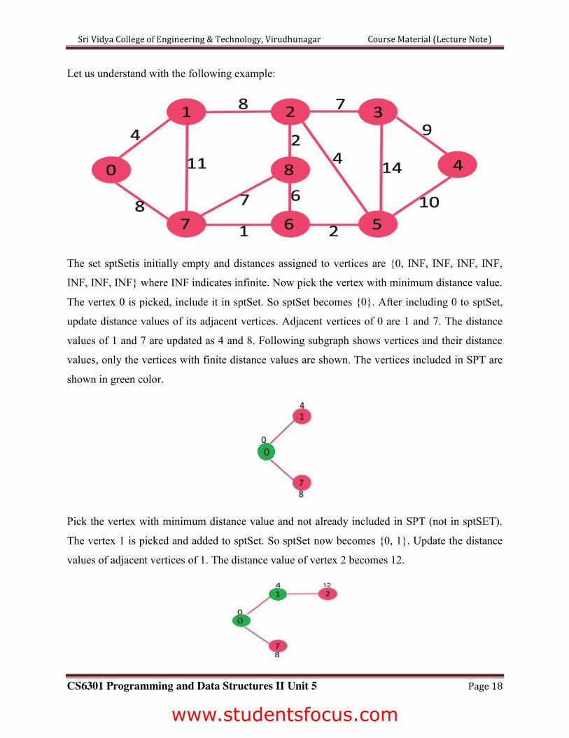
Let us understand with the following example:

The set sptSetis initially empty and distances assigned to vertices are {0, INF, INF, INF, INF,

INF, INF, INF} where INF indicates infinite. Now pick the vertex with minimum distance value.

The vertex 0 is picked, include it in sptSet. So sptSet becomes {0}. After including 0 to sptSet,

update distance values of its adjacent vertices. Adjacent vertices of 0 are 1 and 7. The distance

values of 1 and 7 are updated as 4 and 8. Following subgraph shows vertices and their distance

values, only the vertices with finite distance values are shown. The vertices included in SPT are

shown in green color.

Pick the vertex with minimum distance value and not already included in SPT (not in sptSET).

The vertex 1 is picked and added to sptSet. So sptSet now becomes {0, 1}. Update the distance

values of adjacent vertices of 1. The distance value of vertex 2 becomes 12.





Vertex 7 is picked. So sptSet now becomes {0, 1, 7}. Update the distance values of adjacent

vertices of 7. The distance value of vertex 6 and 8 becomes finite (15 and 9 respectively).


Vertex 6 is picked. So sptSet now becomes {0, 1, 7, 6}. Update the distance values of adjacent

vertices of 6. The distance value of vertex 5 and 8 are updated.

We repeat the above steps until sptSet doesn’t include all vertices of given graph. Finally, we get

the following Shortest Path Tree (SPT).

Bellman–Ford Algorithm

Given a graph and a source vertex src in graph, find shortest paths from src to all vertices in the

given graph. The graph may contain negative weight edges.




We have discussed Dijkstra’s algorithm for this problem. Dijksra’s algorithm is a Greedy

algorithm and time complexity is O(VLogV) (with the use of Fibonacci heap). Dijkstra doesn’t

work for Graphs with negative weight edges, Bellman-Ford works for such graphs. Bellman-

Ford is also simpler than Dijkstra and suites well for distributed systems. But time complexity of

Bellman-Ford is O(VE), which is more than Dijkstra.

Algorithm

Following are the detailed steps.

Input: Graph and a source vertex src

Output: Shortest distance to all vertices from src. If there is a negative weight cycle, then shortest

distances are not calculated, negative weight cycle is reported.

1) This step initializes distances from source to all vertices as infinite and distance to source

itself as 0. Create an array dist[] of size |V| with all values as infinite except dist[src] where src is

source vertex.

2) This step calculates shortest distances. Do following |V|-1 times where |V| is the number of

vertices in given graph.

…..a) Do following for each edge u-v

………………If dist[v] >dist[u] + weight of edge uv, then update dist[v]

………………….dist[v] = dist[u] + weight of edge uv

3) This step reports if there is a negative weight cycle in graph. Do following for each edge u-v

……If dist[v] >dist[u] + weight of edge uv, then “Graph contains negative weight cycle”

The idea of step 3 is, step 2 guarantees shortest distances if graph doesn’t contain negative

weight cycle. If we iterate through all edges one more time and get a shorter path for any vertex,

then there is a negative weight cycle

How does this work? Like other Dynamic Programming Problems, the algorithm calculate

shortest paths in bottom-up manner. It first calculates the shortest distances for the shortest paths




which have at-most one edge in the path. Then, it calculates shortest paths with at-nost 2 edges,

and so on. After the ith iteration of outer loop, the shortest paths with at most i edges are

calculated. There can be maximum |V| – 1 edges in any simple path, that is why the outer loop

runs |v| – 1 times. The idea is, assuming that there is no negative weight cycle, if we have

calculated shortest paths with at most i edges, then an iteration over all edges guarantees to give

shortest path with at-most (i+1) edges.

Example

Let us understand the algorithm with following example graph. The images are taken from this

source.

Let the given source vertex be 0. Initialize all distances as infinite, except the distance to source

itself. Total number of vertices in the graph is 5, so all edges must be processed 4 times.

Let all edges are processed in following order: (B,E), (D,B), (B,D), (A,B), (A,C), (D,C), (B,C),

(E,D). We get following distances when all edges are processed first time. The first row in shows

initial distances. The second row shows distances when edges (B,E), (D,B), (B,D) and (A,B) are

processed. The third row shows distances when (A,C) is processed. The fourth row shows when

(D,C), (B,C) and (E,D) are processed.




The first iteration guarantees to give all shortest paths which are at most 1 edge long. We get

following distances when all edges are processed second time (The last row shows final values).

The second iteration guarantees to give all shortest paths which are at most 2 edges long. The

algorithm processes all edges 2 more times. The distances are minimized after the second

iteration, so third and fourth iterations don’t update the distances.

Floyd–Warshall algorithm

the Floyd–Warshall algorithm (also known as Floyd's algorithm, Roy–Warshall algorithm, Roy–

Floyd algorithm, or the WFI algorithm) is a graph analysis algorithm for finding shortest paths in

a weighted graph with positive or negative edge weights (but with no negative cycles, see below)

and also for finding transitive closure of a relation R. A single execution of the algorithm will




find the lengths (summed weights) of the shortest paths between all pairs of vertices, though it

does not return details of the paths themselves.

The Floyd–Warshall algorithm was published in its currently recognized form by Robert Floyd

in 1962. However, it is essentially the same as algorithms previously published by Bernard Roy

in 1959 and also by Stephen Warshall in 1962 for finding the transitive closure of a graph.[1]

The modern formulation of Warshall's algorithm as three nested for-loops was first described by

Peter Ingerman, also in 1962.

The algorithm is an example of dynamic programming.

1 let dist be a |V| × |V| array of minimum distances initialized to ∞ (infinity)

2 for each vertex v

3 dist[v][v] ← 0

4 for each edge (u,v)

5 dist[u][v] ← w(u,v) // the weight of the edge (u,v)

6 for k from 1 to |V|

7 for i from 1 to |V|

8 for j from 1 to |V|

9 if dist[i][j] >dist[i][k] + dist[k][j]

10 dist[i][j] ← dist[i][k] + dist[k][j]

11 end if

Example

The algorithm above is executed on the graph on the left below:




Prior to the first iteration of the outer loop, labeled k=0 above, the only known paths correspond

to the single edges in the graph. At k=1, paths that go through the vertex 1 are found: in

particular, the path 2→1→3 is found, replacing the path 2→3 which has fewer edges but is

longer. At k=2, paths going through the vertices {1,2} are found. The red and blue boxes show

how the path 4→2→1→3 is assembled from the two known paths 4→2 and 2→1→3

encountered in previous iterations, with 2 in the intersection. The path 4→2→3 is not

considered, because 2→1→3 is the shortest path encountered so far from 2 to 3. At k=3, paths

going through the vertices {1,2,3} are found. Finally, at k=4, all shortest paths are found.


CS6301 Programming and Data Structures...

Documents

Transcript of CS6301 Programming and Data Structures...