CS5620 Geometric Modeling II Intro to Computer Graphics · · 2015-10-05Geometric Modeling II...

CS5620

Intro to Computer Graphics

Copyright

C. Gotsman, G. Elber, M. Ben-Chen

Computer Science Dept., Technion

Geometric Modeling II

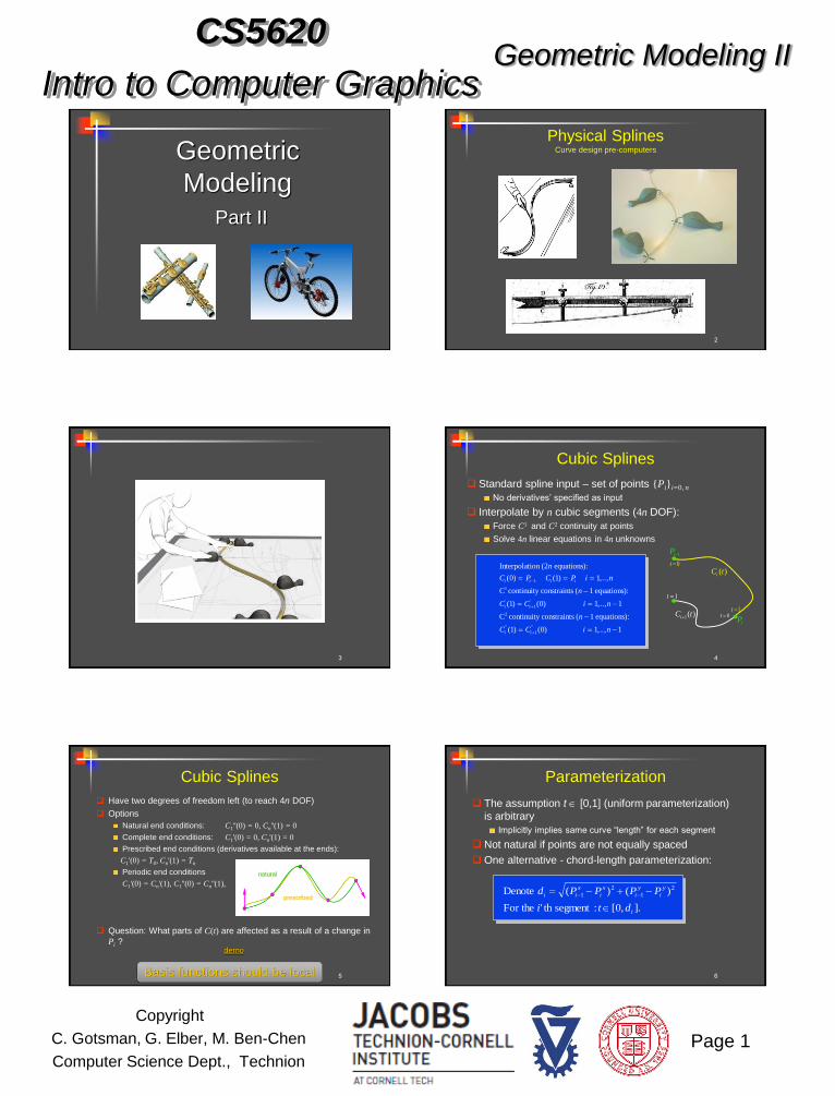
Geometric

Modeling

Part II

2

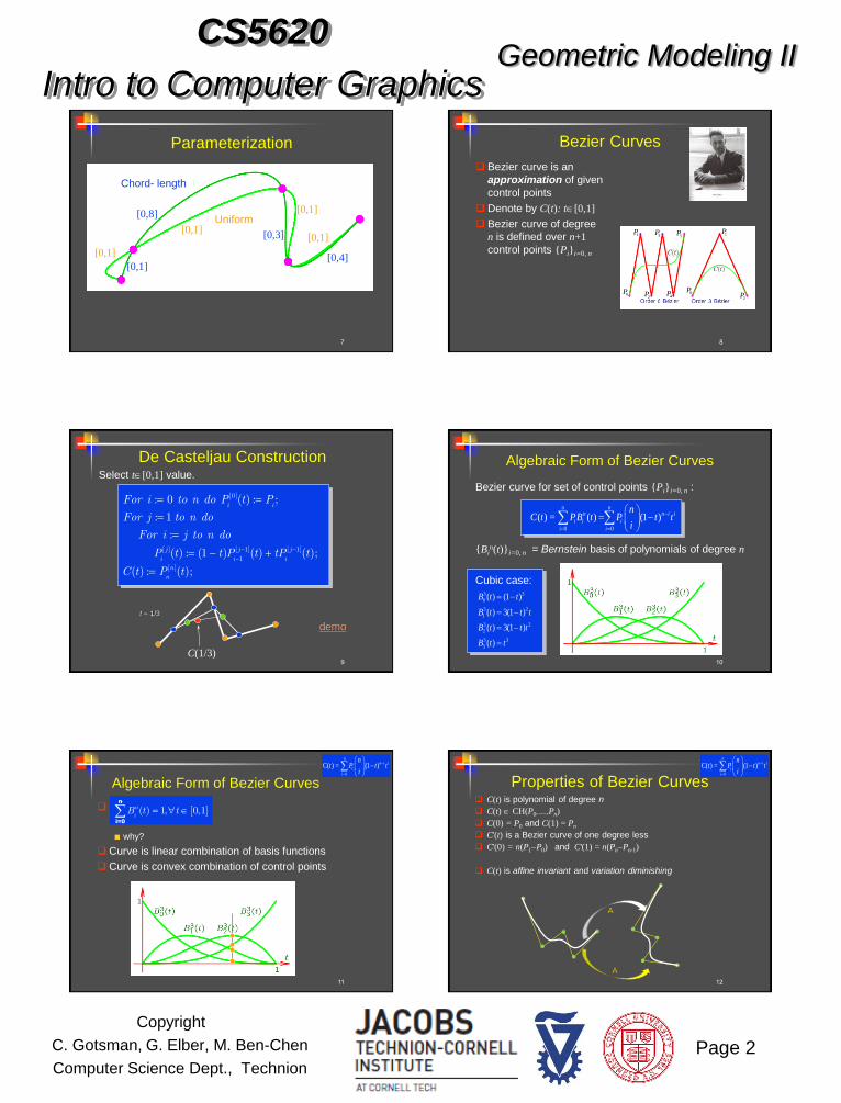
Physical Splines Curve design pre-computers

3 4

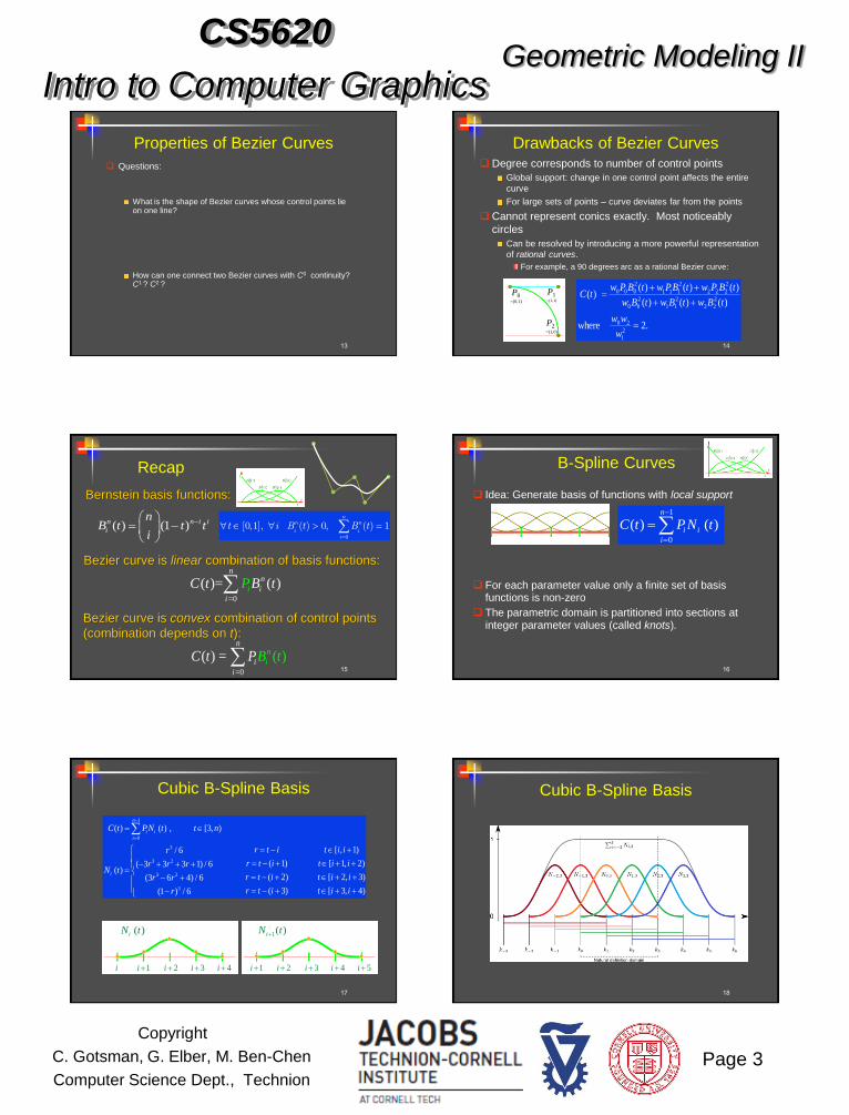
Cubic Splines

Standard spline input – set of points {Pi}i=0, n

No derivatives’ specified as input

Interpolate by n cubic segments (4n DOF):

Force C1 and C2 continuity at points

Solve 4n linear equations in 4n unknowns

Interpolation (2 equations):

C continuity constraints ( equations):

C continuity constraints ( equations):

1

2

n

C P C P i n

n

C C i n

n

C C i n

i i i i

i i

i i

( ) ( ) ,..,

( ) ( ) ,..,

( ) ( ) ,..,

' '

' ' ' '

0 1 1

1

1 0 1 1

1

1 0 1 1

1

1

1

1( )iC t 0t

1t

( )iC t0t

1t

1iP

iP

5

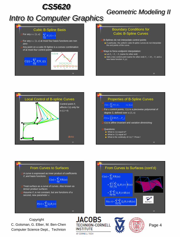
Cubic Splines

Have two degrees of freedom left (to reach 4n DOF)

Options

Natural end conditions: C1''(0) = 0, Cn''(1) = 0

Complete end conditions: C1'(0) = 0, Cn'(1) = 0

Prescribed end conditions (derivatives available at the ends):

C1'(0) = T0, Cn'(1) = Tn

Periodic end conditions

C1'(0) = Cn'(1), C1''(0) = Cn''(1),

Question: What parts of C(t) are affected as a result of a change in

Pi ?

prescribed

natural

demo

Basis functions should be local 6

The assumption t [0,1] (uniform parameterization)

is arbitrary

Implicitly implies same curve “length” for each segment

Not natural if points are not equally spaced

One alternative - chord-length parameterization:

Parameterization

].,0[ :segmentth ' For the

)()( Denote 2

1

2

1

i

y

i

y

i

x

i

x

ii

dti

PPPPd

http://www.cse.unsw.edu.au/~lambert/splines/natcubic.html

CS5620


Copyright




7

Parameterization

Uniform

Chord- length

[0,1]

[0,1]

[0,8]

[0,1]

[0,3]

[0,1]

[0,1]

[0,4]

8

Bezier Curves

Bezier curve is an

approximation of given

control points

Denote by C(t): t[0,1]

Bezier curve of degree

n is defined over n+1

control points {Pi}i=0, n

P1 P3 5P P1

P2

P0P0 P2P4

( )C t

( )C t

9

De Casteljau Construction

[0]

[ ] [ 1] [ 1]

1[ ]

: 0 ( ) : ;

: 1

:

( ) : (1 ) ( ) ( );

( ) : ( );

i i

j j j

i i in

n

For i to n do P t P

For j to n do

For i j to n do

P t t P t tP t

C t P t

C(1/3)

Select t[0,1] value.

t = 1/3

demo

10

Algebraic Form of Bezier Curves

Bezier curve for set of control points {Pi}i=0, n :

{Bin(t)}i=0, n = Bernstein basis of polynomials of degree n

Cubic case:

n

i=0 0

( ) = ( ) (1 )

nn n i i

i i i

i

nC t PB t P t t

i

3 3

0

3 2

1

3 2

2

3 3

3

( ) (1 )

( ) 3(1 )

( ) 3(1 )

( )

B t t

B t t t

B t t t

B t t

11

Algebraic Form of Bezier Curves

why?

Curve is linear combination of basis functions

Curve is convex combination of control points

n

i=0

( ) 1, [0,1]n

iB t t

0

C( ) = (1 )

nn i i

i

i

nt P t t

i

12

Properties of Bezier Curves C(t) is polynomial of degree n

C(t) CH(P0,…,Pn)

C(0) = P0 and C(1) = Pn

C'(t) is a Bezier curve of one degree less

C'(0) = n(P1P0) and C'(1) = n(PnPn-1)

C(t) is affine invariant and variation diminishing

A

A

0

C( ) = (1 )

nn i i

i

i

nt P t t

i

../Zachi/bezier.mov

http://www.vis.uni-stuttgart.de/~kraus/LiveGraphics3D/cagd/chap4fig2.html

CS5620


Copyright




13

Properties of Bezier Curves

Questions:

What is the shape of Bezier curves whose control points lie on one line?

How can one connect two Bezier curves with C0 continuity? C1 ? C2 ?

14

Drawbacks of Bezier Curves Degree corresponds to number of control points

Global support: change in one control point affects the entire

curve

For large sets of points – curve deviates far from the points

Cannot represent conics exactly. Most noticeably

circles

Can be resolved by introducing a more powerful representation

of rational curves.

For example, a 90 degrees arc as a rational Bezier curve:

.2where

)()()(

)()()()(

2

1

20

2

22

2

11

2

00

2

222

2

111

2

000

w

ww

tBwtBwtBw

tBPwtBPwtBPw tCP0

=(0,1)

P1 =(1,1)

P2 =(1,0)

Recap

15

=0

( )= ( )n

n

ii

i

B tPC t

Bezier curve is linear combination of basis functions:

( ) (1 )

n n i i

i

nB t t t

i

Bezier curve is convex combination of control points

(combination depends on t):

=0

( ) = ( ) n

i

n

i

i

C B tt P

Bernstein basis functions:

0

[0,1], ( ) 0, ( ) 1n

n n

i ii

t i B t B t

16

B-Spline Curves

Idea: Generate basis of functions with local support

For each parameter value only a finite set of basis functions is non-zero

The parametric domain is partitioned into sections at integer parameter values (called knots).

1

0

)()(n

i

ii tNPtC

17

Cubic B-Spline Basis

1

0

3

3 2

3 2

3

( ) ( ) , [3, )

[ , 1)/ 6

( 1) [ 1, 2)( 3 3 3 1) / 6( )

( 2) [ 2, 3)(3 6 4) / 6

( 3) [ 3, 4)(1 ) / 6

n

i i

i

i

C t PN t t n

r t i t i ir

r t i t i ir r rN t

r t i t i ir r

r t i t i ir

3( )iN t

1 2 3 4i i i i i

3

1( )iN t

1 2 3 4 5i i i i i

Cubic B-Spline Basis

18

CS5620


Copyright




19

Cubic B-Spline Basis For any t [3, n]:

For any t [3, n] at most four basis functions are non

zero

Any point on a cubic B-Spline is a convex combination

of at most four control points

1

0

( ) 1n

ii

N t

1

0

)()(n

i

ii tNPtC

[3,4)t

0 1 2 3 4 5 6 7

3 3 3 3

0 1 2 3( ) ( ) ( ) ( )N t N t N t N t

20

B-Splines do not interpolate control points

in particular, the uniform cubic B-spline curves do not interpolate

the end points of the curve.

Ways to force endpoint interpolation:

Let P0 = P1 = P2 (same for other end)

Add a new control point (same for other end) P-1 = 2P0 – P1 and a

new basis function N-1(t).

Boundary Conditions for

Cubic B-Spline Curves

21

Local Control of B-spline Curves

Control point Pi

affects C(t) only for

t(i,i+4)

demo

22

Properties of B-Spline Curves

For n control points, C(t) is a piecewise polynomial of

degree 3, defined over t[3, n)

C(t) is affine invariant and variation diminishing

Questions: What is C(i) equal to?

What is C’(i) equal to?

What is the continuity of C(t) ? Prove !

4

30

( ) ( ,.., )n

i ii

C t CH P P

1

0

( ) ( ) , [3, )n

i ii

C t PN t t n

23

From Curves to Surfaces

A curve is expressed as inner product of coefficients

Pi and basis functions

Treat surface as a curve of curves. Also known as

tensor product surfaces

Assume Pi is not constant, but are functions of a

second, new parameter v:

n

i

ii uBPuC0

)()(

m

j

jiji vBQvP0

)()(

24

From Curves to Surfaces (cont’d)

n

i

i

m

j

jij

n

i

i

m

j

jij

n

i

ii

uBvBQ

uBvBQ

uBPuC

0 0

0 0

0

)()(

)()(

)()(

n

i

i

m

j

jij uBvBQvuS0 0

)()(),( BezPatch

http://staff.www.ltu.se/~peppar/presentations/bibdc961114/misc_applets/ParamCurve/

http://www.math.psu.edu/dlittle/java/parametricequations/beziersurfaces/index.html

../Applets/applets/bezpatch/html/index.html

CS5620


Copyright




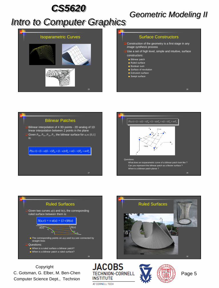
Isoparametric Curves

25 26

Surface Constructors

Construction of the geometry is a first stage in any

image synthesis process

Use a set of high level, simple and intuitive, surface

constructors:

Bilinear patch

Ruled surface

Boolean sum

Surface of revolution

Extrusion surface

Swept surface

27

Bilinear Patches

Bilinear interpolation of 4 3D points - 2D analog of 1D

linear interpolation between 2 points in the plane

Given P00, P01, P10, P11 the bilinear surface for u,v[0,1]

is:

11100100 )1()1()1)(1(),( uvPPvuvPuPvuvuP

28

P10 P11

P00

P10

P01

x

y

Questions:

What does an isoparametric curve of a bilinear patch look like ?

Can you represent the bilinear patch as a Bezier surface ?

When is a bilinear patch planar ?

00 01 10 11( , ) (1 )(1 ) (1 ) (1 )P u v u v P u vP u v P uvP

29

Given two curves a(t) and b(t), the corresponding

ruled surface between them is:

The corresponding points on a(u) and b(u) are connected by

straight lines

Questions:

When is a ruled surface a bilinear patch?

When is a bilinear patch a ruled surface?

Ruled Surfaces

S(u,v) = v a(u) + (1-v)b(u)

a(u) b(u)

u0

u1

u0

u1

Ruled Surfaces

30

CS5620


Copyright




Bridge of Strings

31 32

Boolean Sum

Given four connected curves i i=1,2,3,4, Boolean sum

S(u, v) fills the interior.

Then

)()1()(),(

)()1()(),(

)1(

)1()1)(1(),(

312

201

1110

0100

vuvuvuS

uvuvvuS

uvPPvu

vPuPvuvuP

),(),(),(),( 21 vuPvuSvuSvuS

33

Boolean Sum (cont’d)

S(u,v) interpolates the four

i along its boundaries.

For example, consider the

u = 0 boundary:

)(

)1()()1(

)1()(1)(0)0()1()0(

),0(),0(),0(

),0(

3

010030001

01003120

21

v

vPPvvPvvP

vPPvvvvv

vPvSvS

vS

34

Surface of Revolution Rotate a, usually planar,

curve around an axis

Consider curve

(t) = (x(t), 0, z(t))

and let Z be the axis of

revolution.

( , ) ( ) cos( ),

( , ) ( )sin( ),

( , ) ( ).

x

x

z

x u v u v

y u v u v

z u v u

(t)

Surfaces of Revolution

35 36

Extruded Surface

Extrusion of a, usually

planar, curve along a

linear segment.

Given curve (t) and

vector

( , ) ( )S u v u vV

(t) (t)

V

VV

CS5620


Copyright




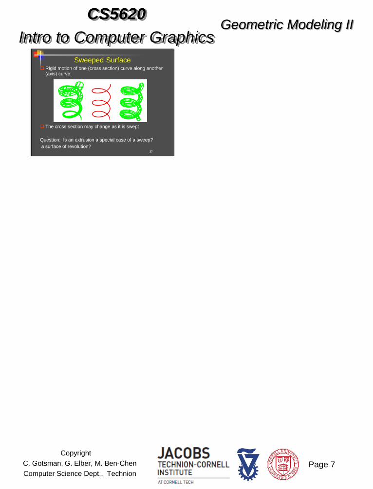
37

Sweeped Surface Rigid motion of one (cross section) curve along another

(axis) curve:

The cross section may change as it is swept

Question: Is an extrusion a special case of a sweep?

a surface of revolution?

CS5620 Geometric Modeling II Intro to Computer Graphics · · 2015-10-05Geometric Modeling II...

Documents

Transcript of CS5620 Geometric Modeling II Intro to Computer Graphics · · 2015-10-05Geometric Modeling II...