
CS224d Deep NLP Lecture 8: Recurrent Neural … NLP Lecture 8: Recurrent Neural Networks Richard...
38
Transcript of CS224d Deep NLP Lecture 8: Recurrent Neural … NLP Lecture 8: Recurrent Neural Networks Richard...
Overview
4/21/16RichardSocher2
• Feedback
• Traditionallanguagemodels
• RNNs
• RNNlanguagemodels
• Importanttrainingproblemsandtricks
• Vanishingandexplodinggradientproblems
• RNNsforothersequencetasks
• BidirectionalanddeepRNNs

Feedback
4/21/16RichardSocher3
Feedbackà Superusefulà Thanks!
4/21/16RichardSocher4
Explaintheintuitionbehindthemathandmodelsmore
à sometoday:)
Givemoreexamples,moretoyexamplesandrecapslidescanhelpusunderstandfaster
à Sometoyexamplestoday.Recapofmainconceptsnextweek
Consistencyissuesindimensionality,rowvs column,etc.
à Allvectorsshouldbecolumnvectors…unlessImessedup,pleasesenderrata
Ilikethequalityoftheproblemsetsandespeciallythestartercode.Itwouldbenicetoincludeballparkvaluesweshouldexpect
àWilladdinfuturePsets andonPiazza.We’llalsoadddimensionality.

FeedbackonProject
4/21/16RichardSocher5
Pleasegivelistofproposedprojects
à
• Greatfeedback,IaskedresearchgroupsatStanfordandwillcompilealistfornextTuesday.
• We’llmoveprojectproposaldeadlinetonextweekThursday.
• Extracreditdeadlinefordataset+firstbaselineisforprojectmilestone.
LanguageModels
4/21/16RichardSocher6
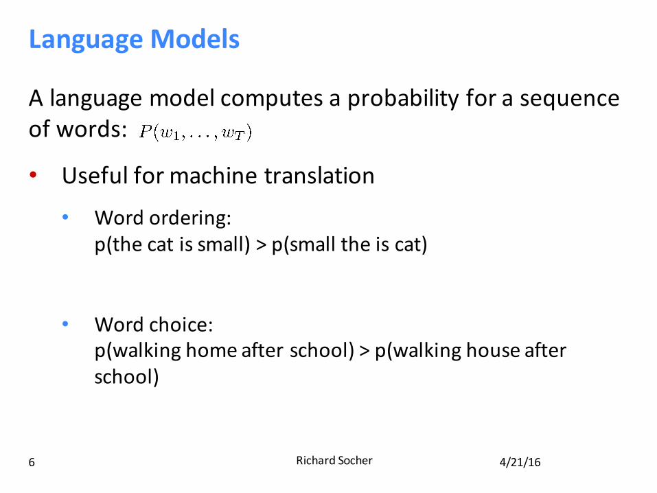
Alanguagemodelcomputesaprobabilityforasequenceofwords:
• Usefulformachinetranslation• Wordordering:
p(thecatissmall)>p(smalltheiscat)
• Wordchoice:p(walkinghomeafterschool)>p(walkinghouseafterschool)
TraditionalLanguageModels
4/21/16RichardSocher7
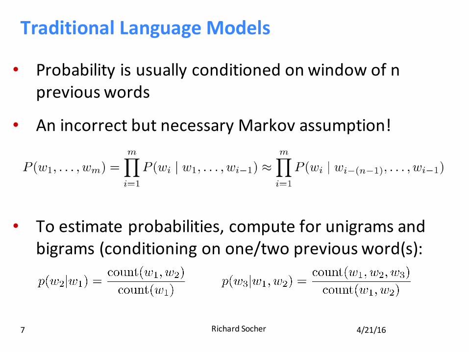
• Probabilityisusuallyconditionedonwindowofnpreviouswords
• AnincorrectbutnecessaryMarkovassumption!
• Toestimateprobabilities,computeforunigramsandbigrams(conditioningonone/twopreviousword(s):
TraditionalLanguageModels
4/21/16RichardSocher8
• Performanceimproveswithkeepingaroundhighern-gramscountsanddoingsmoothingandso-calledbackoff (e.g.if4-gramnotfound,try3-gram,etc)
• ThereareALOTofn-grams!à GiganticRAMrequirements!
• Recentstateoftheart:ScalableModifiedKneser-NeyLanguageModelEstimation byHeafield etal.:“Usingonemachinewith140GBRAMfor2.8days,webuiltanunprunedmodelon126billiontokens”
RecurrentNeuralNetworks!
4/21/16RichardSocher9
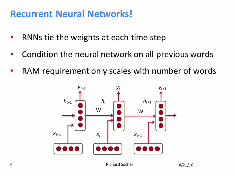
• RNNstietheweightsateachtimestep
• Conditiontheneuralnetworkonallpreviouswords
• RAMrequirementonlyscaleswithnumberofwords
xt−1 xt xt+1
ht−1 ht ht+1W W
yt−1 yt yt+1
RecurrentNeuralNetworklanguagemodel
4/21/16RichardSocher10
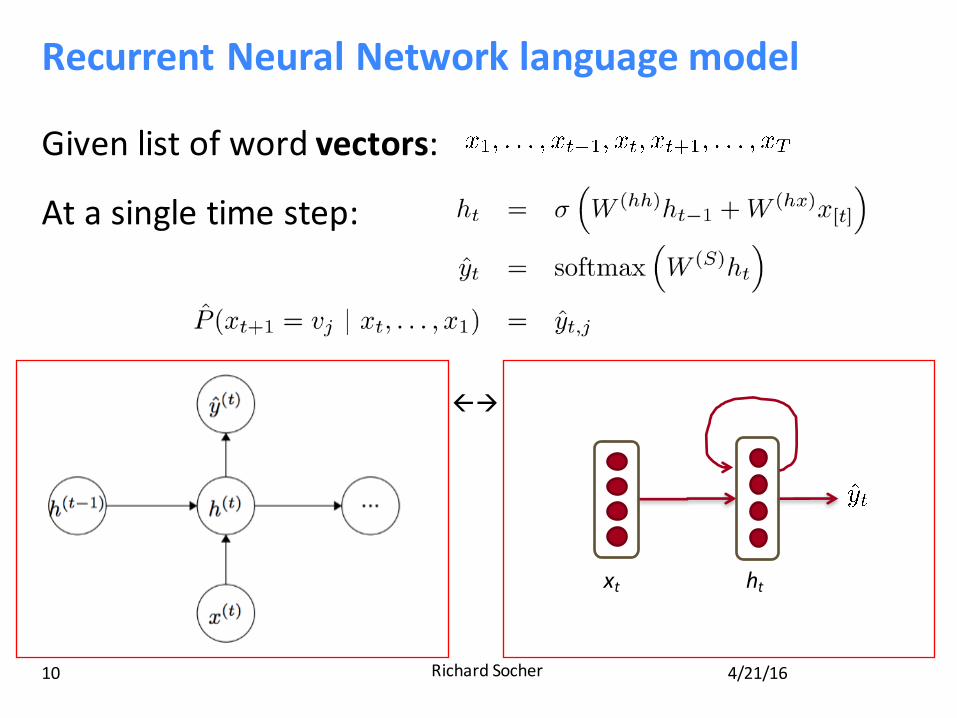
Givenlistofwordvectors:
Atasingletimestep:
xt ht
ßà
RecurrentNeuralNetworklanguagemodel
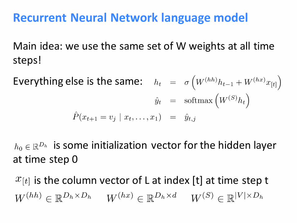
Mainidea:weusethesamesetofWweightsatalltimesteps!
Everythingelseisthesame:
issomeinitializationvectorforthehiddenlayerattimestep0
isthecolumnvectorofLatindex[t]attimestept
RecurrentNeuralNetworklanguagemodel
4/21/16RichardSocher12
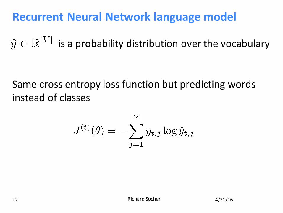
isaprobabilitydistributionoverthevocabulary
Samecrossentropylossfunctionbutpredictingwordsinsteadofclasses
RecurrentNeuralNetworklanguagemodel
4/21/16RichardSocher13
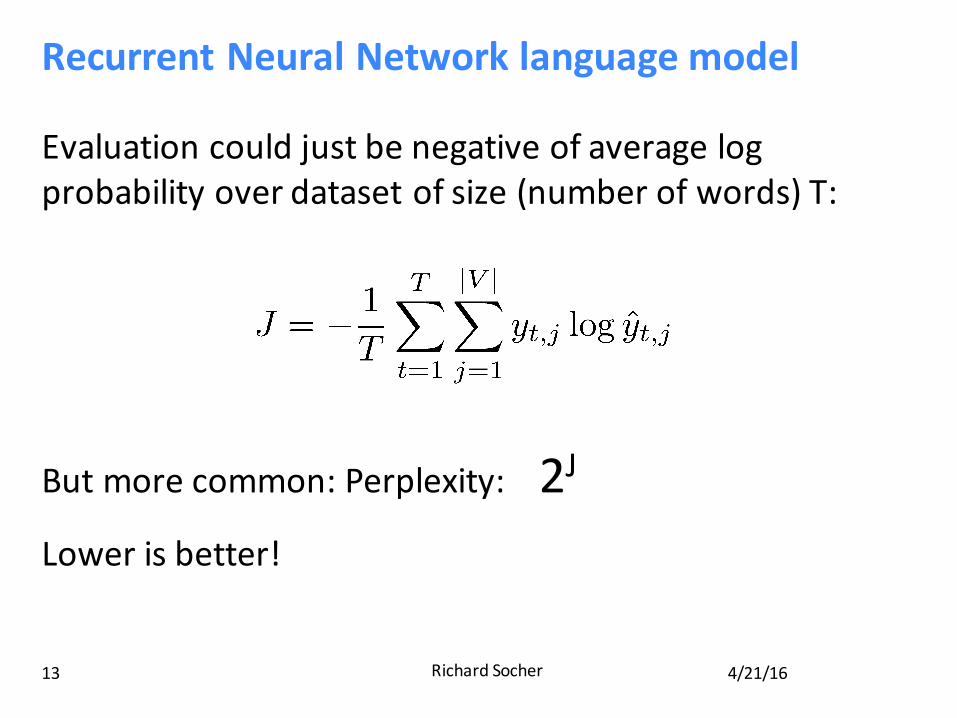
Evaluationcouldjustbenegativeofaveragelogprobabilityoverdatasetofsize(numberofwords)T:
Butmorecommon:Perplexity:2J
Lowerisbetter!
TrainingRNNsishard
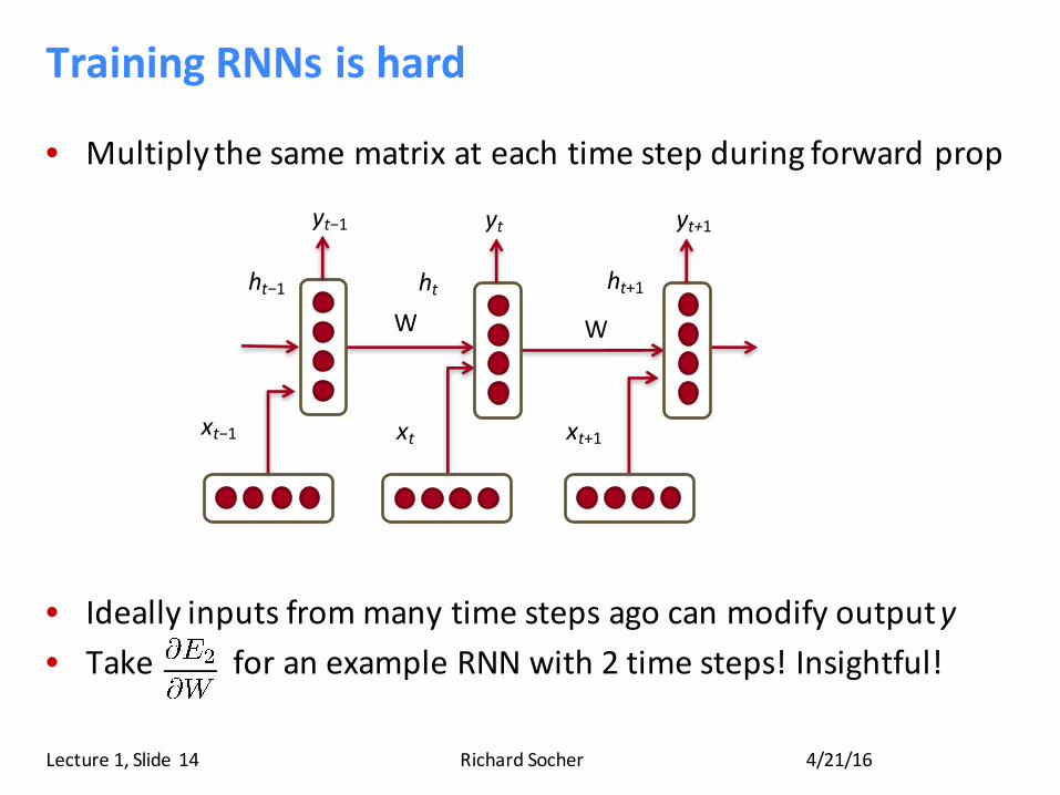
• Multiplythesamematrixateachtimestepduringforwardprop
• Ideallyinputsfrommanytimestepsagocanmodifyoutputy• TakeforanexampleRNNwith2timesteps!Insightful!
4/21/16RichardSocherLecture1,Slide 14
xt−1 xt xt+1
ht−1 ht ht+1W W
yt−1 yt yt+1
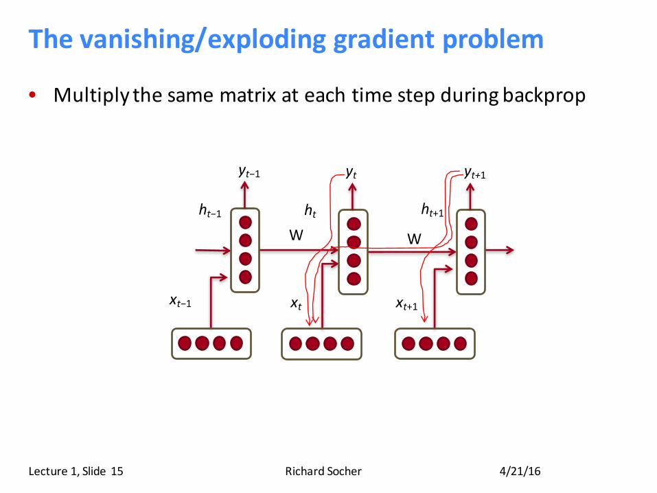
Thevanishing/explodinggradientproblem
• Multiplythesamematrixateachtimestepduringbackprop
4/21/16RichardSocherLecture1,Slide 15
xt−1 xt xt+1
ht−1 ht ht+1W W
yt−1 yt yt+1
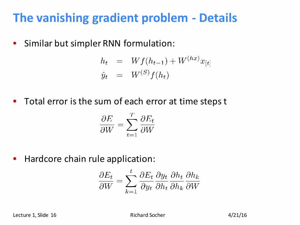
Thevanishinggradientproblem- Details
• SimilarbutsimplerRNNformulation:
• Totalerroristhesumofeacherrorattimestepst
• Hardcorechainruleapplication:
4/21/16RichardSocherLecture1,Slide 16
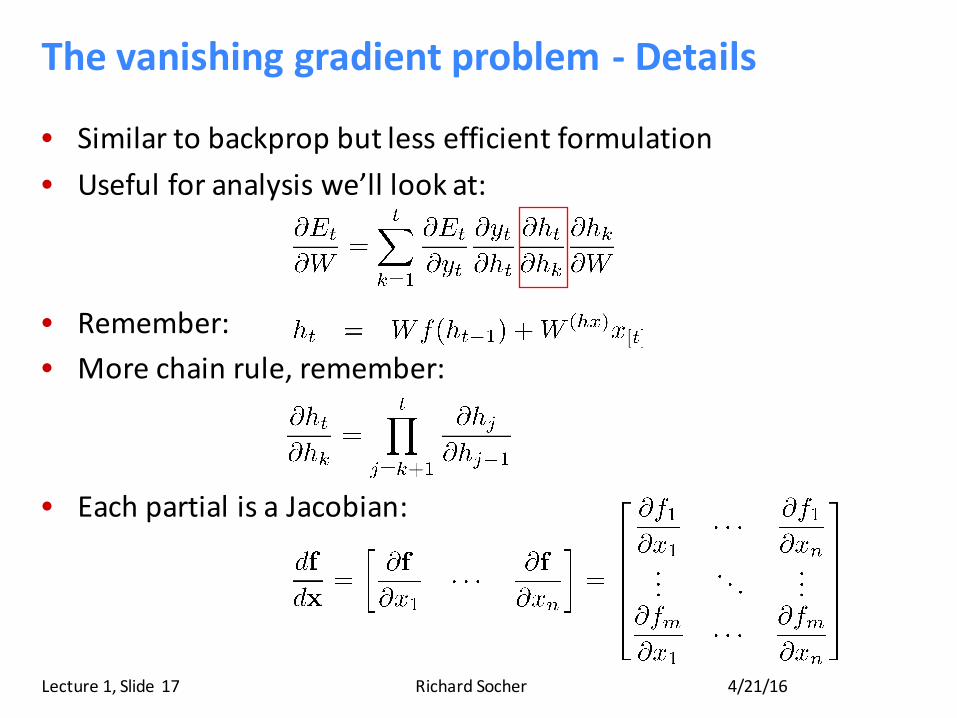
Thevanishinggradientproblem- Details
• Similartobackprop butlessefficientformulation• Usefulforanalysiswe’lllookat:
• Remember:• Morechainrule,remember:
• EachpartialisaJacobian:
4/21/16RichardSocherLecture1,Slide 17
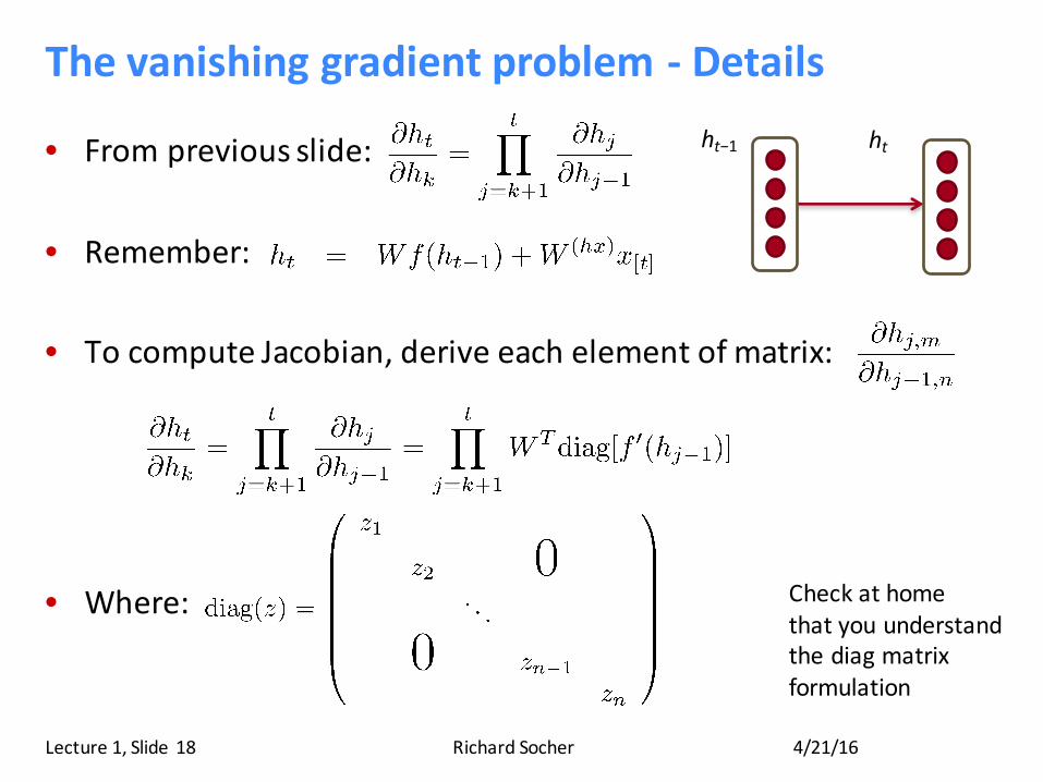
Thevanishinggradientproblem- Details
• Frompreviousslide:
• Remember:
• TocomputeJacobian,deriveeachelement ofmatrix:
• Where:
4/21/16RichardSocherLecture1,Slide 18
ht−1 ht
Checkathomethatyouunderstandthediag matrixformulation
Thevanishinggradientproblem- Details
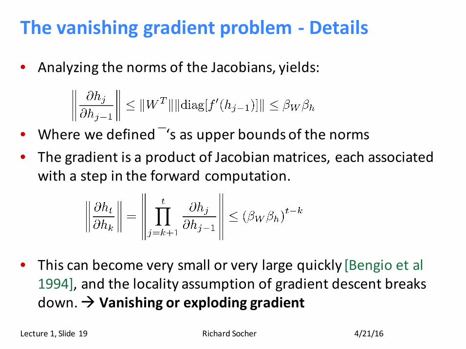
• AnalyzingthenormsoftheJacobians,yields:
• Wherewedefined ‘sasupperboundsofthenorms• ThegradientisaproductofJacobianmatrices,eachassociated
withastepintheforwardcomputation.
• Thiscanbecomeverysmallorverylargequickly[Bengio etal1994],andthelocalityassumptionofgradientdescentbreaksdown.à Vanishingorexplodinggradient
4/21/16RichardSocherLecture1,Slide 19
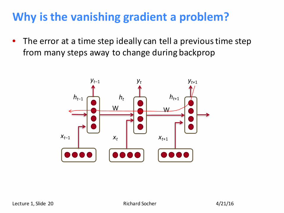
Whyisthevanishinggradientaproblem?
• Theerroratatimestepideallycantellaprevioustimestepfrommanystepsawaytochangeduringbackprop
4/21/16RichardSocherLecture1,Slide 20
xt−1 xt xt+1
ht−1 ht ht+1W W
yt−1 yt yt+1
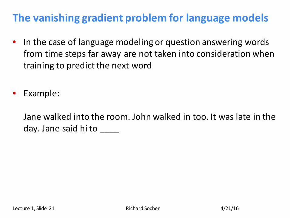
Thevanishinggradientproblemforlanguagemodels
• Inthecaseoflanguagemodelingorquestionansweringwordsfromtimestepsfarawayarenottakenintoconsiderationwhentrainingtopredictthenextword
• Example:
Janewalkedintotheroom.Johnwalkedintoo.Itwaslateintheday.Janesaidhito____
4/21/16RichardSocherLecture1,Slide 21

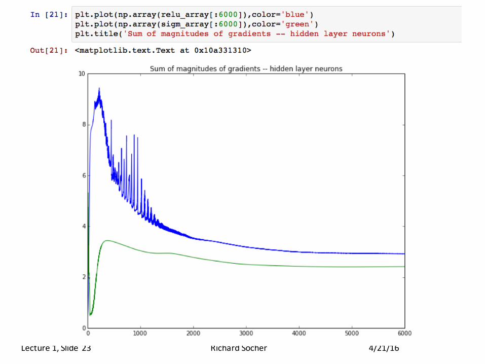
IPython Notebookwithvanishinggradientexample
• ExampleofsimpleandcleanNNet implementation
• ComparisonofsigmoidandReLu units
• Alittlebitofvanishinggradient
4/21/16RichardSocherLecture1,Slide 22
4/21/16RichardSocherLecture1,Slide 23
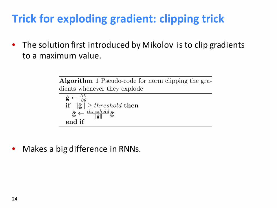
Trickforexplodinggradient:clippingtrick
• ThesolutionfirstintroducedbyMikolov istoclipgradientstoamaximumvalue.
• MakesabigdifferenceinRNNs.
24
On the di�culty of training Recurrent Neural Networks
region of space. It has been shown that in practiceit can reduce the chance that gradients explode, andeven allow training generator models or models thatwork with unbounded amounts of memory(Pascanuand Jaeger, 2011; Doya and Yoshizawa, 1991). Oneimportant downside is that it requires a target to bedefined at every time step.
In Hochreiter and Schmidhuber (1997); Graves et al.(2009) a solution is proposed for the vanishing gra-dients problem, where the structure of the model ischanged. Specifically it introduces a special set ofunits called LSTM units which are linear and have arecurrent connection to itself which is fixed to 1. Theflow of information into the unit and from the unit isguarded by an input and output gates (their behaviouris learned). There are several variations of this basicstructure. This solution does not address explicitly theexploding gradients problem.
Sutskever et al. (2011) use the Hessian-Free opti-mizer in conjunction with structural damping, a spe-cific damping strategy of the Hessian. This approachseems to deal very well with the vanishing gradient,though more detailed analysis is still missing. Pre-sumably this method works because in high dimen-sional spaces there is a high probability for long termcomponents to be orthogonal to short term ones. Thiswould allow the Hessian to rescale these componentsindependently. In practice, one can not guarantee thatthis property holds. As discussed in section 2.3, thismethod is able to deal with the exploding gradientas well. Structural damping is an enhancement thatforces the change in the state to be small, when the pa-rameter changes by some small value�✓. This asks forthe Jacobian matrices @xt
@✓
to have small norm, hencefurther helping with the exploding gradients problem.The fact that it helps when training recurrent neuralmodels on long sequences suggests that while the cur-vature might explode at the same time with the gradi-ent, it might not grow at the same rate and hence notbe su�cient to deal with the exploding gradient.
Echo State Networks (Lukosevicius and Jaeger, 2009)avoid the exploding and vanishing gradients problemby not learning the recurrent and input weights. Theyare sampled from hand crafted distributions. Becauseusually the largest eigenvalue of the recurrent weightis, by construction, smaller than 1, information fed into the model has to die out exponentially fast. Thismeans that these models can not easily deal with longterm dependencies, even though the reason is slightlydi↵erent from the vanishing gradients problem. Anextension to the classical model is represented by leakyintegration units (Jaeger et al., 2007), where
x
k
= ↵x
k�1 + (1� ↵)�(Wrec
x
k�1 +W
in
u
k
+ b).
While these units can be used to solve the standardbenchmark proposed by Hochreiter and Schmidhu-ber (1997) for learning long term dependencies (see(Jaeger, 2012)), they are more suitable to deal withlow frequency information as they act as a low passfilter. Because most of the weights are randomly sam-pled, is not clear what size of models one would needto solve complex real world tasks.
We would make a final note about the approach pro-posed by Tomas Mikolov in his PhD thesis (Mikolov,2012)(and implicitly used in the state of the art re-sults on language modelling (Mikolov et al., 2011)).It involves clipping the gradient’s temporal compo-nents element-wise (clipping an entry when it exceedsin absolute value a fixed threshold). Clipping has beenshown to do well in practice and it forms the backboneof our approach.
3.2. Scaling down the gradients
As suggested in section 2.3, one simple mechanism todeal with a sudden increase in the norm of the gradi-ents is to rescale them whenever they go over a thresh-old (see algorithm 1).
Algorithm 1 Pseudo-code for norm clipping the gra-dients whenever they explode
g @E@✓
if kgk � threshold then
g threshold
kgk g
end if
This algorithm is very similar to the one proposed byTomas Mikolov and we only diverged from the originalproposal in an attempt to provide a better theoreticalfoundation (ensuring that we always move in a de-scent direction with respect to the current mini-batch),though in practice both variants behave similarly.
The proposed clipping is simple to implement andcomputationally e�cient, but it does however in-troduce an additional hyper-parameter, namely thethreshold. One good heuristic for setting this thresh-old is to look at statistics on the average norm overa su�ciently large number of updates. In our ex-periments we have noticed that for a given task andmodel size, training is not very sensitive to this hyper-parameter and the algorithm behaves well even forrather small thresholds.
The algorithm can also be thought of as adaptingthe learning rate based on the norm of the gradient.Compared to other learning rate adaptation strate-gies, which focus on improving convergence by col-lecting statistics on the gradient (as for example in
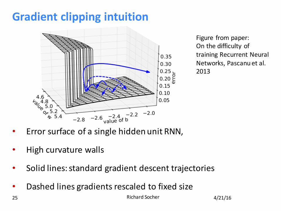
Gradientclippingintuition
4/21/16RichardSocher25
• ErrorsurfaceofasinglehiddenunitRNN,
• Highcurvaturewalls
• Solidlines:standardgradientdescenttrajectories
• Dashedlinesgradientsrescaledtofixedsize
On the di�culty of training Recurrent Neural Networks
Figure 6. We plot the error surface of a single hidden unit
recurrent network, highlighting the existence of high cur-
vature walls. The solid lines depicts standard trajectories
that gradient descent might follow. Using dashed arrow
the diagram shows what would happen if the gradients is
rescaled to a fixed size when its norm is above a threshold.
explode so does the curvature along v, leading to awall in the error surface, like the one seen in Fig. 6.
If this holds, then it gives us a simple solution to theexploding gradients problem depicted in Fig. 6.
If both the gradient and the leading eigenvector of thecurvature are aligned with the exploding direction v, itfollows that the error surface has a steep wall perpen-dicular to v (and consequently to the gradient). Thismeans that when stochastic gradient descent (SGD)reaches the wall and does a gradient descent step, itwill be forced to jump across the valley moving perpen-dicular to the steep walls, possibly leaving the valleyand disrupting the learning process.
The dashed arrows in Fig. 6 correspond to ignoringthe norm of this large step, ensuring that the modelstays close to the wall. The key insight is that all thesteps taken when the gradient explodes are alignedwith v and ignore other descent direction (i.e. themodel moves perpendicular to the wall). At the wall, asmall-norm step in the direction of the gradient there-fore merely pushes us back inside the smoother low-curvature region besides the wall, whereas a regulargradient step would bring us very far, thus slowing orpreventing further training. Instead, with a boundedstep, we get back in that smooth region near the wallwhere SGD is free to explore other descent directions.
The important addition in this scenario to the classicalhigh curvature valley, is that we assume that the val-ley is wide, as we have a large region around the wallwhere if we land we can rely on first order methodsto move towards the local minima. This is why justclipping the gradient might be su�cient, not requiringthe use a second order method. Note that this algo-
rithm should work even when the rate of growth of thegradient is not the same as the one of the curvature(a case for which a second order method would failas the ratio between the gradient and curvature couldstill explode).
Our hypothesis could also help to understand the re-cent success of the Hessian-Free approach comparedto other second order methods. There are two key dif-ferences between Hessian-Free and most other second-order algorithms. First, it uses the full Hessian matrixand hence can deal with exploding directions that arenot necessarily axis-aligned. Second, it computes anew estimate of the Hessian matrix before each up-date step and can take into account abrupt changes incurvature (such as the ones suggested by our hypothe-sis) while most other approaches use a smoothness as-sumption, i.e., averaging 2nd order signals over manysteps.
3. Dealing with the exploding andvanishing gradient
3.1. Previous solutions
Using an L1 or L2 penalty on the recurrent weights canhelp with exploding gradients. Given that the parame-ters initialized with small values, the spectral radius ofW
rec
is probably smaller than 1, from which it followsthat the gradient can not explode (see necessary condi-tion found in section 2.1). The regularization term canensure that during training the spectral radius neverexceeds 1. This approach limits the model to a sim-ple regime (with a single point attractor at the origin),where any information inserted in the model has to dieout exponentially fast in time. In such a regime we cannot train a generator network, nor can we exhibit longterm memory traces.
Doya (1993) proposes to pre-program the model (toinitialize the model in the right regime) or to useteacher forcing. The first proposal assumes that ifthe model exhibits from the beginning the same kindof asymptotic behaviour as the one required by thetarget, then there is no need to cross a bifurcationboundary. The downside is that one can not alwaysknow the required asymptotic behaviour, and, even ifsuch information is known, it is not trivial to initial-ize a model in this specific regime. We should alsonote that such initialization does not prevent cross-ing the boundary between basins of attraction, which,as shown, could happen even though no bifurcationboundary is crossed.
Teacher forcing is a more interesting, yet a not verywell understood solution. It can be seen as a way ofinitializing the model in the right regime and the right
Figure frompaper:OnthedifficultyoftrainingRecurrentNeuralNetworks,Pascanuetal.2013
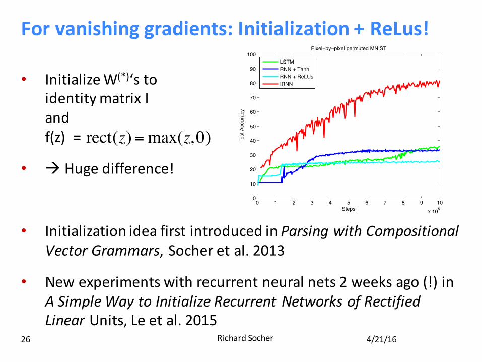
Forvanishinggradients:Initialization+ReLus!
4/21/16RichardSocher26
• InitializeW(*)‘stoidentitymatrixIandf(z)=
• à Hugedifference!
• InitializationideafirstintroducedinParsingwithCompositionalVectorGrammars,Socheretal.2013
• Newexperimentswithrecurrentneuralnets2weeksago(!)inASimpleWaytoInitializeRecurrentNetworksofRectifiedLinearUnits,Leetal.2015
T LSTM RNN + Tanh IRNN150 lr = 0.01, gc = 10, fb = 1.0 lr = 0.01, gc = 100 lr = 0.01, gc = 100
200 lr = 0.001, gc = 100, fb = 4.0 N/A lr = 0.01, gc = 1
300 lr = 0.01, gc = 1, fb = 4.0 N/A lr = 0.01, gc = 10
400 lr = 0.01, gc = 100, fb = 10.0 N/A lr = 0.01, gc = 1
Table 1: Best hyperparameters found for adding problems after grid search. lr is the learning rate, gcis gradient clipping, and fb is forget gate bias. N/A is when there is no hyperparameter combinationthat gives good result.
4.2 MNIST Classification from a Sequence of Pixels
Another challenging toy problem is to learn to classify the MNIST digits [21] when the 784 pixelsare presented sequentially to the recurrent net. In our experiments, the networks read one pixel at atime in scanline order (i.e. starting at the top left corner of the image, and ending at the bottom rightcorner). The networks are asked to predict the category of the MNIST image only after seeing all784 pixels. This is therefore a huge long range dependency problem because each recurrent networkhas 784 time steps.
To make the task even harder, we also used a fixed random permutation of the pixels of the MNISTdigits and repeated the experiments.
All networks have 100 recurrent hidden units. We stop the optimization after it converges or whenit reaches 1,000,000 iterations and report the results in figure 3 (best hyperparameters are listed intable 2).
0 1 2 3 4 5 6 7 8 9 10x 105
0
10
20
30
40
50
60
70
80
90
100
Steps
Test
Acc
urac
y
Pixel−by−pixel MNIST
LSTMRNN + TanhRNN + ReLUsIRNN
0 1 2 3 4 5 6 7 8 9 10x 105
0
10
20
30
40
50
60
70
80
90
100
Steps
Test
Acc
urac
y
Pixel−by−pixel permuted MNIST
LSTMRNN + TanhRNN + ReLUsIRNN
Figure 3: The results of recurrent methods on the “pixel-by-pixel MNIST” problem. We report thetest set accuracy for all methods. Left: normal MNIST. Right: permuted MNIST.
Problem LSTM RNN + Tanh RNN + ReLUs IRNNMNIST lr = 0.01, gc = 1 lr = 10
−8, gc = 10 lr = 10−8, gc = 10 lr = 10
−8, gc = 1
fb = 1.0
permuted lr = 0.01, gc = 1 lr = 10−8, gc = 1 lr = 10
−6, gc = 10 lr = 10−9, gc = 1
MNIST fb = 1.0
Table 2: Best hyperparameters found for pixel-by-pixelMNIST problems after grid search. lr is thelearning rate, gc is gradient clipping, and fb is the forget gate bias.
The results using the standard scanline ordering of the pixels show that this problem is so difficultthat standard RNNs fail to work, even with ReLUs, whereas the IRNN achieves 3% test error ratewhich is better than most off-the-shelf linear classifiers [21]. We were surprised that the LSTM didnot work as well as IRNN given the various initialization schemes that we tried. While it still possi-ble that a better tuned LSTM would do better, the fact that the IRNN perform well is encouraging.
5
rect(z) =max(z, 0)
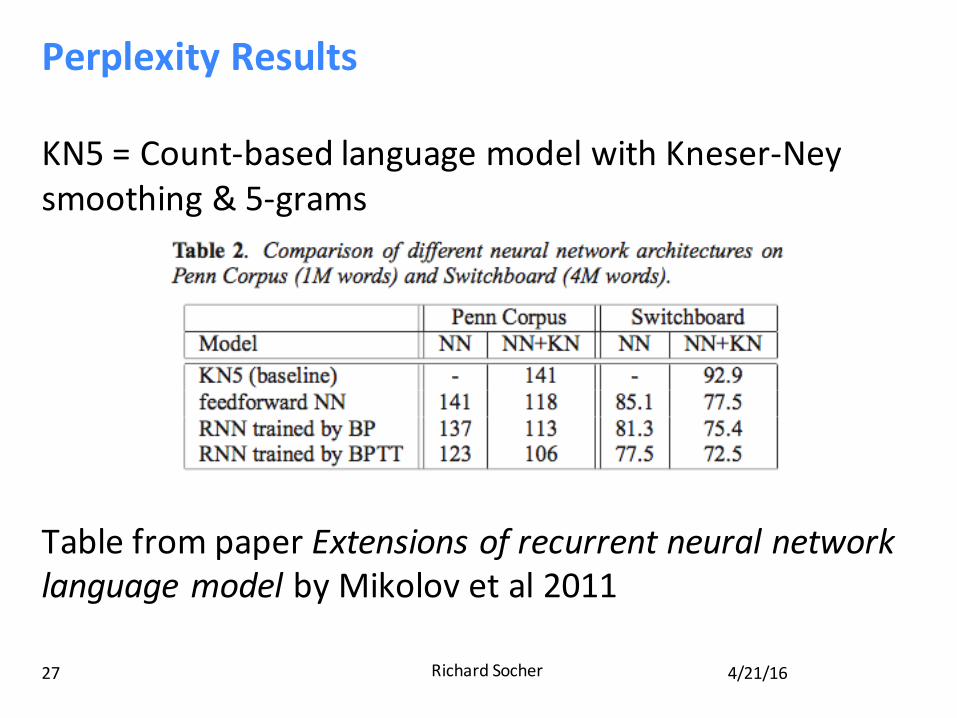
PerplexityResults
4/21/16RichardSocher27
KN5=Count-basedlanguagemodelwithKneser-Neysmoothing&5-grams
TablefrompaperExtensionsofrecurrentneuralnetworklanguagemodel byMikolov etal2011
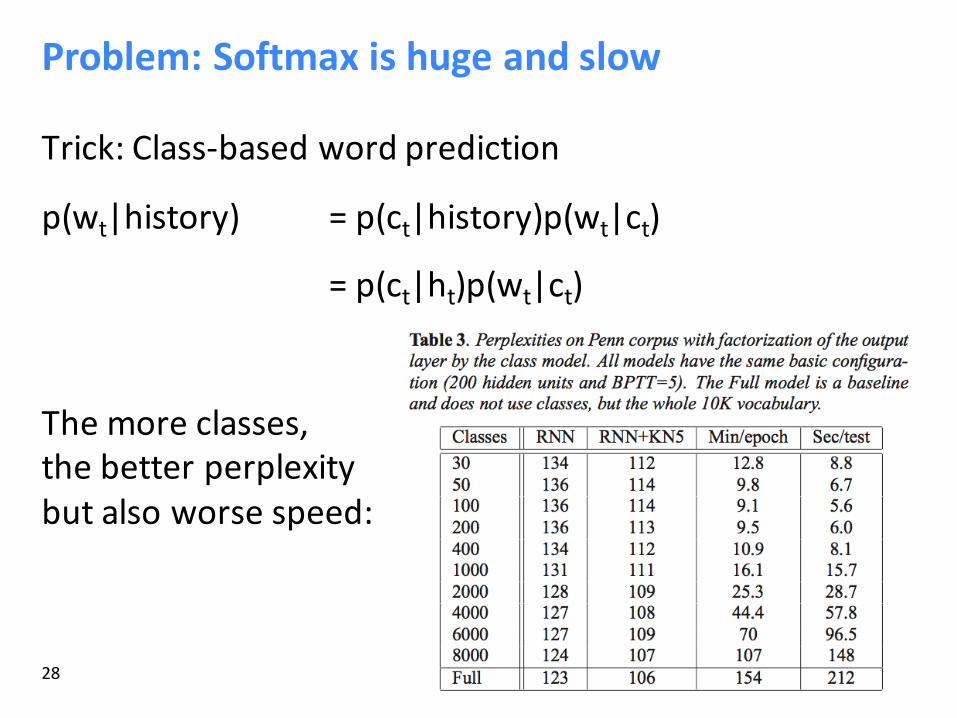
Problem:Softmax ishugeandslow
4/21/16RichardSocher28
Trick:Class-basedwordprediction
p(wt|history) =p(ct|history)p(wt|ct)
=p(ct|ht)p(wt|ct)
Themoreclasses,thebetterperplexitybutalsoworsespeed:

Onelastimplementationtrick
4/21/16RichardSocher29
• YouonlyneedtopassbackwardsthroughyoursequenceonceandaccumulateallthedeltasfromeachEt
Sequencemodelingforothertasks
4/21/16RichardSocher30
• Classifyeachwordinto:• NER
• Entitylevelsentimentincontext
• opinionatedexpressions
• ExampleapplicationandslidesfrompaperOpinionMiningwithDeepRecurrentNetsbyIrsoy andCardie2014
OpinionMiningwithDeepRecurrentNets
4/21/16RichardSocher31
Goal:Classifyeachwordas
directsubjectiveexpressions(DSEs)andexpressivesubjectiveexpressions(ESEs).
DSE:Explicitmentionsofprivatestatesorspeecheventsexpressingprivatestates
ESE:Expressionsthatindicatesentiment,emotion,etc.withoutexplicitlyconveyingthem.
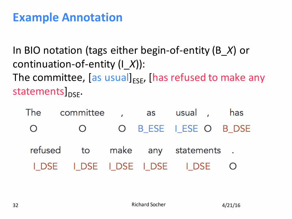
ExampleAnnotation
4/21/16RichardSocher32
InBIOnotation(tagseitherbegin-of-entity(B_X)orcontinuation-of-entity(I_X)):Thecommittee,[asusual]ESE,[hasrefusedtomakeanystatements]DSE.
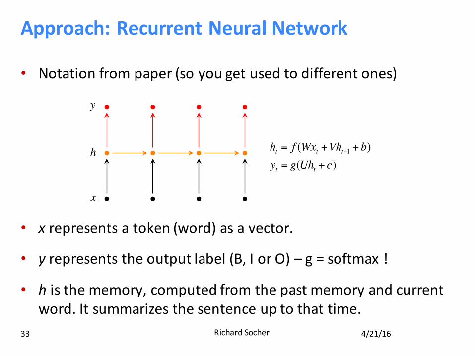
Approach:RecurrentNeuralNetwork
4/21/16RichardSocher33
• Notationfrompaper(soyougetusedtodifferentones)
• xrepresentsatoken(word)asavector.
• yrepresentstheoutputlabel(B,IorO) – g=softmax !
• histhememory,computedfromthepastmemoryandcurrentword.Itsummarizesthesentenceuptothattime.
Recurrent Neural Network
ht = f (Wxt +Vht−1 + b)yt = g(Uht + c)
y
h
x
represents a token (word) as a vector. represents the output label (B, I or O). is the memory, computed from the past memory and current word. It summarizes the sentence up to that time.
xyh
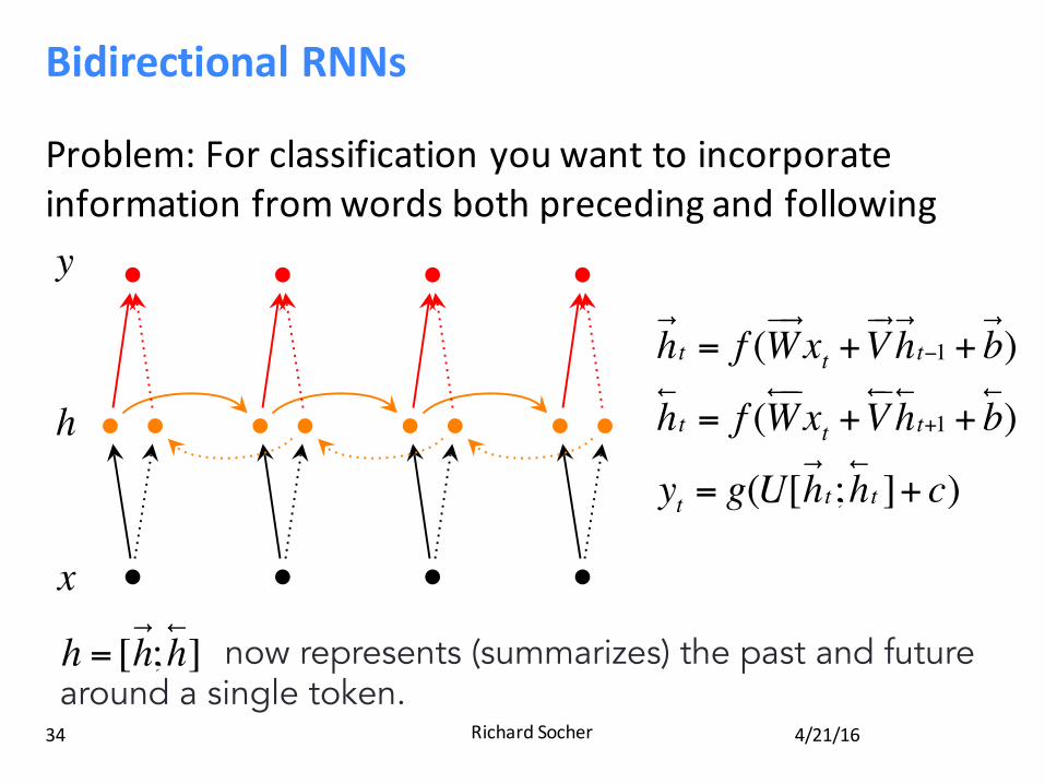
BidirectionalRNNs
4/21/16RichardSocher34
Problem:Forclassificationyouwanttoincorporateinformationfromwordsbothprecedingandfollowing
Ideas?
Bidirectionality
h!t = f (W
!"!xt +V!"h!t−1 + b!)
h!t = f (W
!""xt +V!"h!t+1 + b!)
yt = g(U[h!t;h!t ]+ c)
y
h
x
now represents (summarizes) the past and future around a single token. h = [h!;h!]
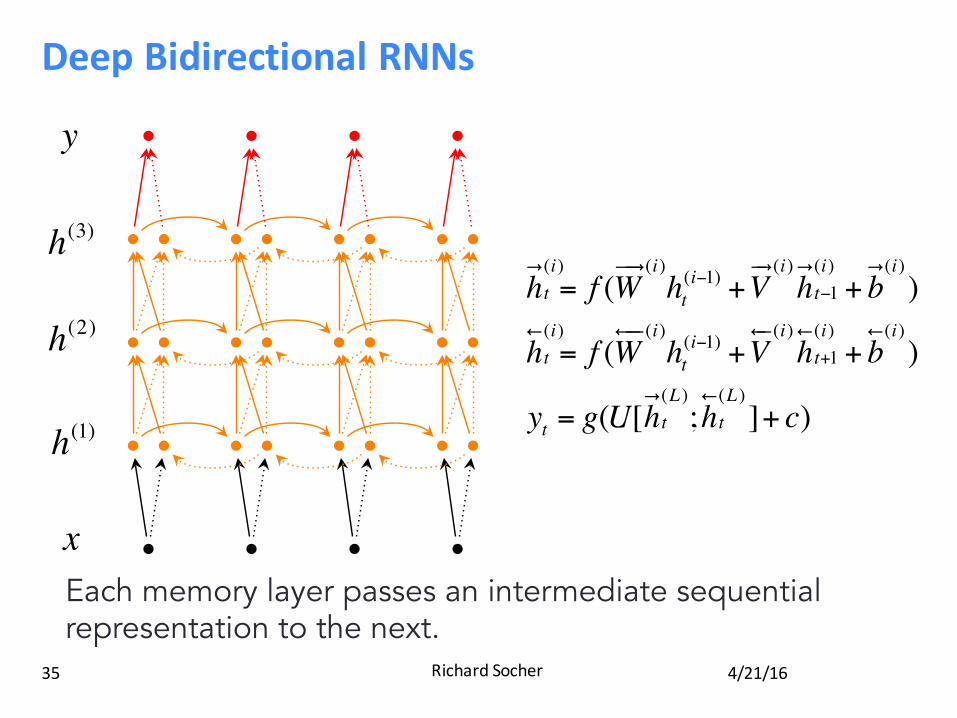
DeepBidirectionalRNNs
4/21/16RichardSocher35
Going Deep
h! (i)t = f (W
!"! (i)ht(i−1) +V
!" (i)h! (i)t−1 + b! (i))
h! (i)t = f (W
!"" (i)ht(i−1) +V
!" (i)h! (i)t+1 + b! (i))
yt = g(U[h!t(L );h!t(L )]+ c)
y
h(3)
xEach memory layer passes an intermediate sequential representation to the next.
h(2)
h(1)
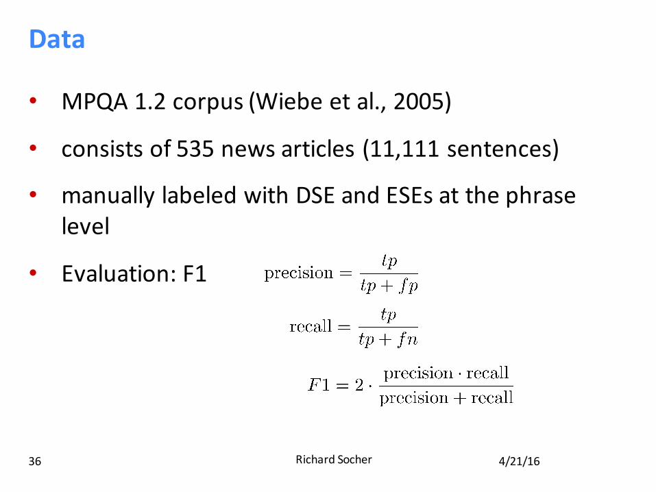
Data
4/21/16RichardSocher36
• MPQA1.2corpus(Wiebe etal.,2005)
• consistsof535newsarticles(11,111sentences)
• manuallylabeledwithDSEandESEsatthephraselevel
• Evaluation:F1
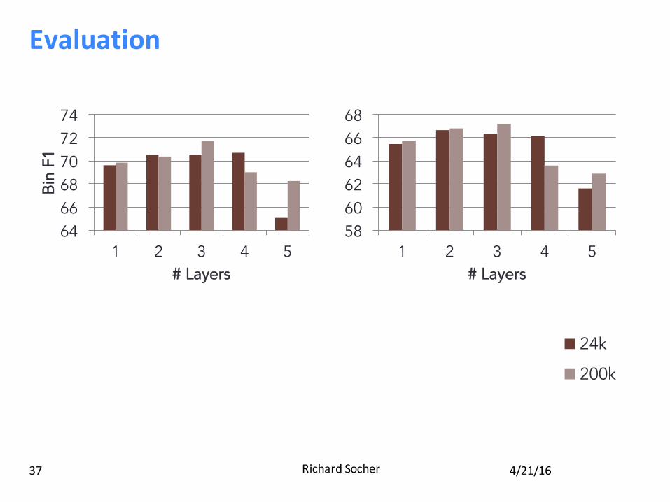
Evaluation
4/21/16RichardSocher37
Results: Deep vs Shallow RNNs
57
59
61
63
65
67
Prop
F1
DSE
64 66 68 70 72 74
1 2 3 4 5
Bin
F1
# Layers
47
49
51
53
55
57 ESE
24k
200k
58 60 62 64 66 68
1 2 3 4 5 # Layers
Results: Deep vs Shallow RNNs
57
59
61
63
65
67
Prop
F1
DSE
64 66 68 70 72 74
1 2 3 4 5
Bin
F1
# Layers
47
49
51
53
55
57 ESE
24k
200k
58 60 62 64 66 68
1 2 3 4 5 # Layers
Recap
4/21/16RichardSocher38
• RecurrentNeuralNetworkisoneofthebestdeepNLPmodelfamilies
• Trainingthemishardbecauseofvanishingandexplodinggradientproblems
• Theycanbeextendedinmanywaysandtheirtrainingimprovedwithmanytricks(moretocome)
• Nextweek:MostimportantandpowerfulRNNextensionswithLSTMsandGRUs


