CS 664 Lecture 6Edge and Corner Detection,

Gaussian Filtering

Prof. Dan HuttenlocherFall 2003

2

Edge Detection

Convert a gray or color image into set of curves– Represented as

binary image

Capture properties of shapes

3

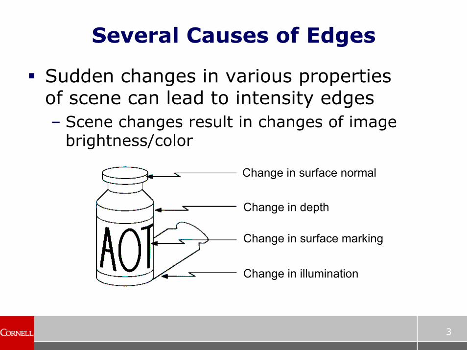
Several Causes of Edges

Sudden changes in various properties of scene can lead to intensity edges– Scene changes result in changes of image

brightness/color

Change in surface normal

Change in depth

Change in surface marking

Change in illumination

4

Detecting Edges

Seek sudden changes in intensity– Various derivatives of image

Idealized continuous image I(x,y)Gradient (first derivative), vector valued

∇I = (∂I/∂x, ∂I/∂y)Squared gradient magnitude

∇I2 = (∂I/∂x)2 + (∂I/∂y)2

– Avoid computing square root

Laplacian (second derivative)∇2I = ∂2I/∂x2 + ∂2I/∂y2

5

The Gradient

Direction of most rapid change

Gradient direction is atan(∂I/∂y,∂I/∂x)– Normal to edge

Strength of edge given by grad magnitude– Often use squared magnitude to avoid

computing square roots

∇I = (∂I/∂x, 0)

∇I = (0, ∂I/∂y)∇I = (∂I/∂x, ∂I/∂y)

6

Finite Differences

Images are digitized– Idealized continuous underlying function I(x,y)

realized as discrete values on a grid I[u,v]

Approximations to derivatives (1D)dF/dx ≈ F[u+1] – F[u]d2F/dx2 ≈ F[u-1] – 2F[u] + F[u+1]

Second derivative symmetric about edge

1 0 1 0 10 11 11 0 1

dF: edge at extremum-1 1 -1 10 1 0 -11 1 0

d2F: edge at zero crossing-2 2 -2 11 -9 -1 -11 12 -2

7

Discrete Gradient

Partial derivatives are estimated at boundaries between adjacent pixels– E.g., pixel and next one in x,y directions

Yields estimates at different points in each direction if use x,y directions

Generally use 45° directions to solve this– Magnitude fine, but gradient orientation needs

to be rotated to correspond to axes

0011

2 1 2

1 12 1 2

3223

8

Estimating Discrete Gradient

Gradient at u,v with 45° axes– Down-right: ∂I/∂x’ ≈ I[u+1,v+1]-I[u,v]– Down-left: ∂I/∂y’ ≈ I[u,v+1]-I[u+1,v]

Handle image border, e.g., no change

u,v

u+1,v+1

u+1,v

u,v+1

6677

2 1 1

1 72 2 7

2676

110-1

4 6 5

1 -10 0 0

0000

-5-4-10

0 6 5

0 -50 0 0

5100

2617

1116 72 50

1 260 0 0

25100

I2∂I/∂x’ ∂I/∂y’I

9

Discrete Laplacian

Laplacian at u,v∂2I/∂x2 = I[u-1,v]-2I[u,v]+I[u+1,v]∂2I/∂y2 = I[u,v-1]-2I[u,v]+I[u,v+1]∇2I is sum of directional second derivatives:I[u-1,v]+I[u+1,v]+I[u,v-1]+I[u,v+1]-4I[u,v]

Can view as 3x3 mask or stencil– Value at u,v given by sum of product with I

Grid yields poor rotational symmetry– Weighted sum of two masks

1 -4 11

1 1-20

11

144

44

1-411

1

10

Local Edge Detectors

Historically several local edge operators based on derivatives– Simple local weighting over small set of pixels

For example Sobel operator– Derivatives in x and y– Weighted sum– 3x3 mask for symmetry– Today can do better with larger masks, fast

algorithms, faster computers

-1

1

-1

1

-2

2-1

1-1

1-2 2

11

Problems With Local Detectors

1D example illustrates effect of noise (variation) on local measures

12

Regions of Support

Desirable to have edge detectors that operate over interval or regionLow pass filtering of an image– Combining certain neighboring pixel values to

produce “less variable” image– Often referred to as “smoothing” or as

“blurring” the image

Simple idea: mean filter – average values over w by h neighborhood

M[u,v] = (1/wh) Σi Σj F[u+i-(w-1)/2, v+j-(h-1)/2]

13

3x3 Mean Filter Example

0000000000

00000009000

0000000000

009090909090000

00909090090000

009090909090000

009090909090000

009090909090000

0000000000

0000000000

??????????

?00000101010?

?1020303030302010?

?204060505030200?

?306090808050300?

?306090808050300?

?306090909060300?

?204060606040200?

?102030303020100?

??????????

M[u,v] = (1/9) Σi Σj F[u+i-1, v+j-1]

14

Border Pixels

As usual with image operations the border cases need to be handled somehow– Produce smaller image by summing only when

entire w by h window fits inside image– Sum only value inside image but produce full

size image• In effect summing zeroes outside image

– Assume value outside image some non-zero value• E.g., reflected copy of the image

No right answer, reflection often least bad

15

Weighted Average Filter

Sum of product with weights HG[u,v] = Σi Σj H[i,j]F[u+i-(w-1)/2, v+j-(h-1)/2]

Mean filter simply has H[I,j]=1/wh– Uniform weighting

Note that entries of H should sum to 1– Otherwise performs overall scaling of the

image• Consider 3x3 mask of 1’s instead of 1/9’s

When averaging generally give central pixel most weight

16

Gaussian Filter

Gaussian in two-dimensions

Weights center moreFalls off smoothlyIntegrates to 1Larger σ produces moreequal weights (blurs more)Normal distribution

17

Gaussian Versus Mean Filter

Mean filter blursbut sharp changes remain as well– “Blocky”

Gaussian notblocky lookingSame areamasks– But Gaussian

small at borders

18

Cross Correlation

The weighted summation operation is called the cross correlation

G[u,v] = Σi Σj H[i,j]F[u+i-(w-1)/2, v+j-(h-1)/2]– Written as G = H⊗F

• Notation not consistent, sometimes written as G = H F, but we will use that for convolution

Powerful operation – Every element of output G results from sum of

product of two inputs H and F– Elements of output differ in shift of inputs H,F– Not that easy to grasp at first

19

Cross Correlation Examples

000

010

000

00000

0ihg0

0fed0

0cba0

00000

?????

?ihg?

?fed?

?cba?

?????

⊗

A

ihg

fed

cba

00000

00000

00100

00000

00000

B

?????

?abc?

?def?

?ghi?

?????

G

⊗

B

GA

20

Convolution

Closely related operation that “flips” indices of H and FG[u,v] = Σi Σj H[i,j]F[u-i+(w-1)/2, v-j+(h-1)/2]– Written as G = H F

• Again, notation not always consistent

Note and ⊗ same when H or F symmetric– I.e., unchanged when “flipped”

Convolution has nice properties– Commutative: A B=B A– Associative: A (B C)=(A B) C– Distributive: A (B+C)=(A B)+(A C)

21

Convolution Examples

000

010

000

00000

0ihg0

0fed0

0cba0

00000

?????

?ihg?

?fed?

?cba?

?????

A

ihg

fed

cba

00000

00000

00100

00000

00000

B

?????

?ihg?

?fed?

?cba?

?????

G

B

GA

22

Identity for Convolution

Unit impulse: one at origin, zero elsewhereSuggests why simple averaging produces “blocky” results– Consider a=b=… =i=K

ihg

fed

cba

00000

00000

00100

00000

00000

?????

?ihg?

?fed?

?cba?

?????

23

Back to Edges: Derivatives

Smooth and then take derivative– 1D example

24

Derivatives and Convolutions

Another useful identity for convolution is d/dx(A B)= (d/dx A) B = A (d/dx B)– Use to skip one step in edge detection

25

Derivatives Using Convolution

When smoothing all weights of mask h are positive– Sum to 1– Maximum weight at center of mask

Weights do not have to all be positive– Negative weights compute differences

(derivatives)– E.g., Laplacian h =– h f = ∇2f

Symmetry of h also gives us h f=h⊗f– True for many masks; makes people sloppy

1-20

11

144

44

26

Linear Operators

Linear shift invariant (LSI) system– Given a “black box” h:

– Linearity:

– Shift invariance:

Convolution with arbitrary h equivalent to these properties– Beyond this course to show it

Linearity is “simple to understand” but real world not always linear– E.g., saturation effects

f h g

af1+bf2 h ag1+bg2

f(x-u) h g(x-u)

27

Area of Support for 2D Operators

Directional first derivatives and second derivative (Laplacian) of Gaussian– Sigma controls scale, larger yields fewer edges

Derivative of Gaussian Laplacian of Gaussian

28

Gradient Magnitude

Also use smoothed image

∇(I hσ) = ((∂(I hσ)/∂x)2 + (∂(I hσ)/∂y)2).5

29

Edge Detection by Subtraction

Difference of image and smoothed version

Difference (brightened)Original Smoothed

30

What Does This Do?

Gaussian

Laplacian of Gaussian

Impulse

More generally (I hσ1)-(I hσ2) ≈ ∇2I(I hσ3)

31

Efficient Gaussian Smoothing

The 2D Gaussian is decomposable into separate 1D convolutions in x and yFirst note that product of two one-dimensional Gaussians

Can view as product of two 1d vectors– Column vector times row vector each with

values of 1d (sampled) Gaussian

32

Expressing as 1D Convolutions

Use unit impulse as a notational trick– Continuous case: δ(x) = ∞ when x is 0, else 0– Discrete case: δ[x] = 1 when x is 0, else 0– f δ=f

hσ = hσx hσy

hσ I = (hσx hσy) I=hσx (hσy I)– Two 1D convolutions, don’t sum the zeroes!

33

2D Gaussian as 1D Convolutions

00000

01616160

01616160

01616160

00000

1/161/81/16

1/81/41/8

1/161/81/16

1/41/21/4

1/4

1/2

1/4

00000

01616160

01616160

01616160

00000

04440

01212120

01616160

01212120

04440

=

=

13431

391293

41216124

391293

13431

=

34

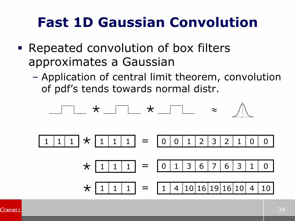
Fast 1D Gaussian Convolution

Repeated convolution of box filters approximates a Gaussian– Application of central limit theorem, convolution

of pdf’s tends towards normal distr.

≈

104101619161041

013676310

001232100111 111 =

111 =

111 =

35

Good Approximation to Gaussian

Convolution of 4 unit height box filters of different widths yields low error– Wells, PAMI Mar 1986

Simply apply each box filter separately– Also separate horizontal and vertical passes– Each box filter constant time per pixel

• Running sum

For Gaussian of given σ– Choose widths wi such that Σi (wi

2-1)/12 ≈ σ2

In practice faster than explicit Gσ for σ ≈ 2

36

What Makes Good Edge Detector

Goals for an edge detector– Minimize probability of multiple detection

• Two pixels classified as edges corresponding to single underlying edge in image

– Minimize probability of false detection– Minimize distance between reported edge and

true edge location

Canny analyzes in detail 1D step edge– Shows that derivative of Gaussian is optimal

with respect to above criteria– Analysis does not extend easily to 2D

37

Canny Edge Detector

Based on gradient magnitude and direction of Gaussian smoothed image– Magnitude: ∇(Gσ I)– Direction (unit vector): ∇(Gσ I) /∇(Gσ I)

Ridges in gradient magnitude– Peaks in direction of gradient (normal to edge)

but not along edge

Hysteresis mechanism for thresholding strong edges– Ridge pixel above lo threshold– Connected via ridge to pixel above hi threshold

38

Canny Edge Definition

Let (δx,δy) = ∇(Gσ I) /∇(Gσ I)– Note compute without explicit square root

Let m = ∇(Gσ I)2

Non-maximum suppression (NMS)– m(x,y) >m(x+δx(x,y),y+δy(x,y))– m(x,y) ≥ m(x-δx(x,y),y-δy(x,y))– Select “ridge points”

Still leaves many candidate edge pixels– E.g., σ=1

39

Canny Thresholding

Two level thresholding of candidate edge pixels (those that survive NMS)– Above lo and connected to pixel above hi

Start by keeping (classifying as edges) all candidates above hi threshold– Recursively if pixel above

lo threshold and adjacent to an edge pixel keep it

Perform recursion using bfs/dfs– E.g., σ=1, lo=5, hi=10 and lo=10, hi=20

40

Corners

Corner characterized by region with intensity change in two different directions

Use local derivative estimates– Gradient oriented in different directions

Not as simple as looking at gradient (partial derivatives) wrt coordinate frame

41

Corner Detectors

Most detectors use local gradient estimate Ix=∂I/∂x and Iy=∂I/∂y– Aggregated over rectangular region

Seek substantial component to gradient in 2 distinct directions– Do so by finding coordinate axes normal to

primary gradient direction

Also detects textured regions

(∂I/∂x, ∂I/∂y)

(∂I/∂x’, 0)

42

Best Coordinate Frame

Eigenvectors of scatter matrix

Major axis of points (Ix,Iy) in “gradient plane” – one for each pixel in regionOrthogonal basis that best characterizes major elongation of points– Geometric view of eigenvector with largest

eigenvalue

Σ Ix2 Σ IxIy

ΣIy2Σ IxIy

C =

43

Simple Corner Detector

Smooth image slightlyCompute derivatives on 45° rotated axis– Eigenvectors thus oriented wrt that grid– Eigenvalues not affected

Find eigenvalues λ1,λ2 of C (λ1<λ2 )– If both large then high gradient in multiple

directions• When λ1 larger than threshold detect a corner

– Eigenvalues can be computed in closed forma bb c

λ1= ½(a+c-√(a-c)2+4b2)

λ2= ½(a+c+√(a-c)2+4b2)

44

Corner Detectors

Two most widely used– KLT (Kanade-Lucas-Tomasi) and Harris

Both based on computing eigenvectors of scatter matrix of partial derivatives– Over some rectangular region

Each has means of ensuring corners not too near one another– Enforcing distance between “good” regions

KLT addresses change between image pair– Important for tracking corners across time

45

KLT Corner Detector

Processing steps1. Compute Ix Iy locally at each pixel

• Perhaps smooth image slightly first

2. For each pixel compute C over d by d neighborhood centered around that pixel– Use box sum for all additions Ix

2, Iy2, IxIy

3. Compute smallest eigenvalue λ1 of C at each pixel

4. Select pixels above some threshold, in order of decreasing magnitude– Omit any pixel that is contained in

neighborhood of previously included pixel

46

KLT Corner Detector Examples

KLT corner detection and tracking code available on the Web robotics.stanford.edu/~birch/klt/

47

Image Sub-Sampling

To halve the resolution of an image seems natural to discard every other row & col– However produces poor looking results

48

Filter then Sub-Sample

Phenomenon known as aliasing– Need to remove high spatial frequencies

• Can’t be represented accurately at lower resolution

• E.g., 000111000111000111000111000• Downsample by 2: 00100100100100• Downsample by 4: 0100100• Downsample by 8: 0010

Nyquist rate: need at least two samples per period of alternating signalAddress by smoothing (lowpass filter)

49

Gaussian Filter and Sub-Sample

50

Gaussian Pyramid

Filter and subsample at each level– Uses only 1/3 more storage than original

51

Sampling and Interpolation

What if scale is not halving of the imageWhat if want to upsample not downsampleMore general issue of constructing best samples on one grid given another grid– Often referred to as resampling

If scaling down, first lowpass filterIn both cases then map from one grid to another– Bilinear interpolation (2 by 2)– Bicubic interpolation (usually 4 by 4)

52

1D Linear Interpolation

Compute intermediate values by weighted combination of neighboring values– Can view as convolution with “hat” on the

original grid• E.g., equal spacing yields mask .5 .5

1 2 3 4 52.5

.5 .5

1 2 3 4 52.75

.25

.75

53

Linear Interpolation by Convolution

Implement by convolution with mask based on grid shift– If grid shifted to right by amount 0<a<1 then

use mask [(1-a) a]

For example grid shifted halfway between

Upsampled

246684420.5 .5

35676431

6 6 5 478 6 3 264443210

54

Bilinear Interpolation

Value at (a,b) based on four neighbors(1 - b) (1 - a) F0,0 + (1 - b) a F1, 0+ b (1 - a) F0,1 + b a F1, 0

55

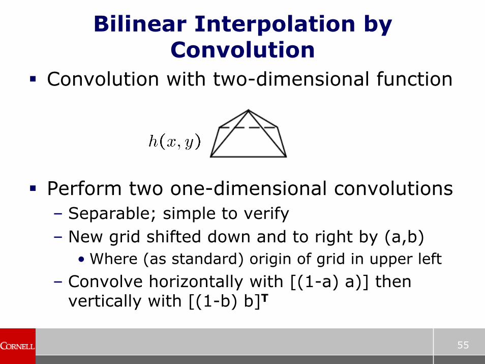
Bilinear Interpolation by Convolution

Convolution with two-dimensional function

Perform two one-dimensional convolutions– Separable; simple to verify– New grid shifted down and to right by (a,b)

• Where (as standard) origin of grid in upper left

– Convolve horizontally with [(1-a) a)] then vertically with [(1-b) b]T

56

Comparing Sampling Methods

Bilinear filter and subsample, Gaussian filter and subsample, straight subsample

Bicubic works better– Can also be implemented as convolution

1/2

1/4