CS 6375: Machine Learning Computational Learning Theoryvgogate/ml/2014f/lectures/colt.pdf · CS...
40
CS 6375: Machine Learning Computational Learning Theory Vibhav Gogate The University of Texas at Dallas Some slides borrowed from Ray Mooney 1
Transcript of CS 6375: Machine Learning Computational Learning Theoryvgogate/ml/2014f/lectures/colt.pdf · CS...
CS 6375: Machine Learning Computational Learning Theory
Vibhav Gogate The University of Texas at Dallas
Some slides borrowed from Ray Mooney
1
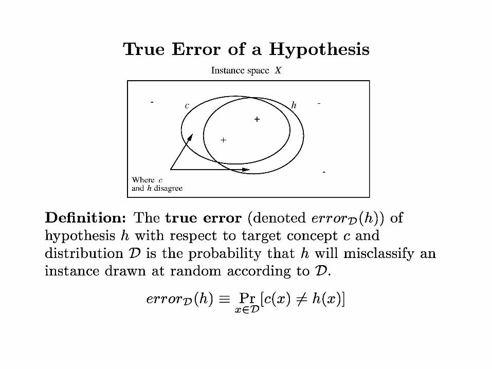
Learning Theory
• Theoretical characterizations of
– Difficulty of several types of ML problems
– Capabilities of several types of ML algorithms
• Questions:
– Under what conditions is successful ML possible and impossible?
– Under what conditions will a particular ML algorithm perform successfully?
2
Learning Theory
• Theorems that characterize – classes of learning problems or
– specific algorithms in terms of • computational complexity or
• sample complexity, i.e. the number of training examples necessary or sufficient to learn hypotheses of a given accuracy.
• Complexity of a learning problem depends on: – Size or expressiveness of the hypothesis space.
– Accuracy to which target concept must be approximated.
– Probability with which the learner must produce a successful hypothesis.
– Manner in which training examples are presented, e.g. randomly or by query to an oracle.
3
Types of Results
• We will not focus on specific learning algorithms but rather on broad classes of ML algorithms characterized by their hypothesis spaces, the presentation of training examples, etc.
• Sample Complexity: How many training examples are needed for a learner to construct (with high probability) a highly accurate concept?
• Computational Complexity: How much computational resources (time and space) are needed for a learner to construct (with high probability) a highly accurate concept? – High sample complexity implies high computational complexity, since
learner at least needs to read the input data.
• Mistake Bound: Learning incrementally, how many training examples will the learner misclassify before constructing a highly accurate concept.
4
Is Perfect Learning possible?
• Number of training examples needed to learn a hypothesis h for which error(h)=0
• Futile:
– There may be multiple hypotheses that are consistent with the training data and the learner cannot be certain to pick the one that equals the target concept
– Since training data is drawn randomly, there is always a chance that the training examples are misleading!
8
9
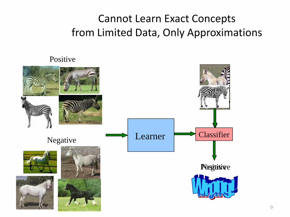
Cannot Learn Exact Concepts from Limited Data, Only Approximations
Negative
Learner Classifier
Positive
Negative
Positive
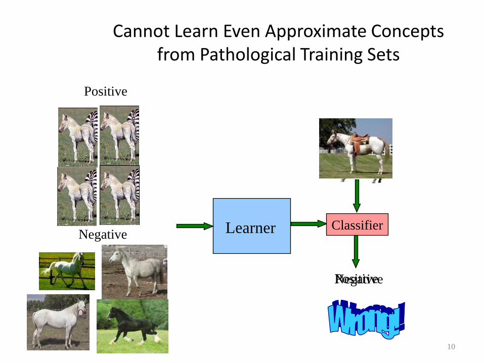
10
Cannot Learn Even Approximate Concepts from Pathological Training Sets
Learner Classifier Negative
Positive
Negative Positive
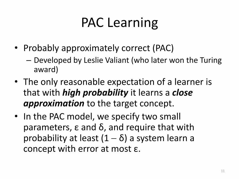
PAC Learning
• Probably approximately correct (PAC) – Developed by Leslie Valiant (who later won the Turing
award)
• The only reasonable expectation of a learner is that with high probability it learns a close approximation to the target concept.
• In the PAC model, we specify two small parameters, ε and δ, and require that with probability at least (1 δ) a system learn a concept with error at most ε.
11
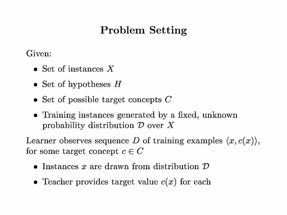
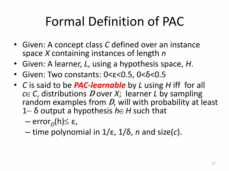
Formal Definition of PAC
• Given: A concept class C defined over an instance space X containing instances of length n
• Given: A learner, L, using a hypothesis space, H. • Given: Two constants: 0<ε<0.5, 0<δ<0.5 • C is said to be PAC-learnable by L using H iff for all
cC, distributions D over X; learner L by sampling random examples from D, will with probability at least 1 δ output a hypothesis hH such that – errorD(h) ε, – time polynomial in 1/ε, 1/δ, n and size(c).
15
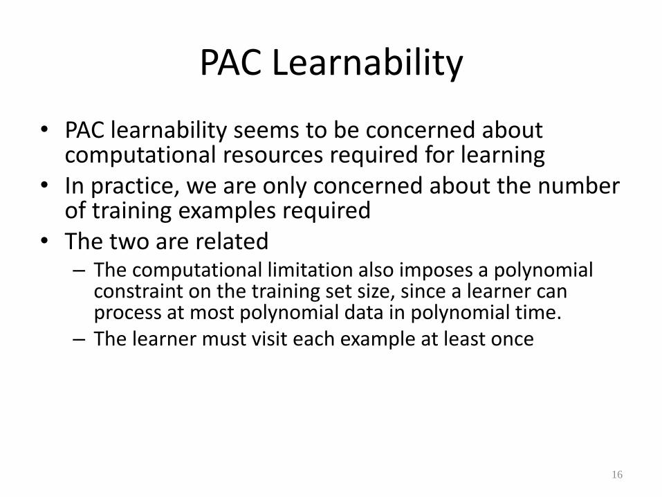
PAC Learnability
• PAC learnability seems to be concerned about computational resources required for learning
• In practice, we are only concerned about the number of training examples required
• The two are related – The computational limitation also imposes a polynomial
constraint on the training set size, since a learner can process at most polynomial data in polynomial time.
– The learner must visit each example at least once
16
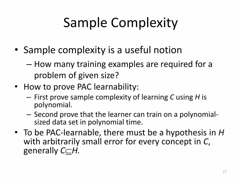
Sample Complexity
• Sample complexity is a useful notion
– How many training examples are required for a problem of given size?
• How to prove PAC learnability: – First prove sample complexity of learning C using H is
polynomial. – Second prove that the learner can train on a polynomial-
sized data set in polynomial time.
• To be PAC-learnable, there must be a hypothesis in H with arbitrarily small error for every concept in C, generally CH.
17
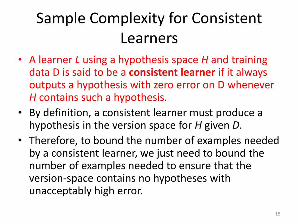
Sample Complexity for Consistent Learners
• A learner L using a hypothesis space H and training data D is said to be a consistent learner if it always outputs a hypothesis with zero error on D whenever H contains such a hypothesis.
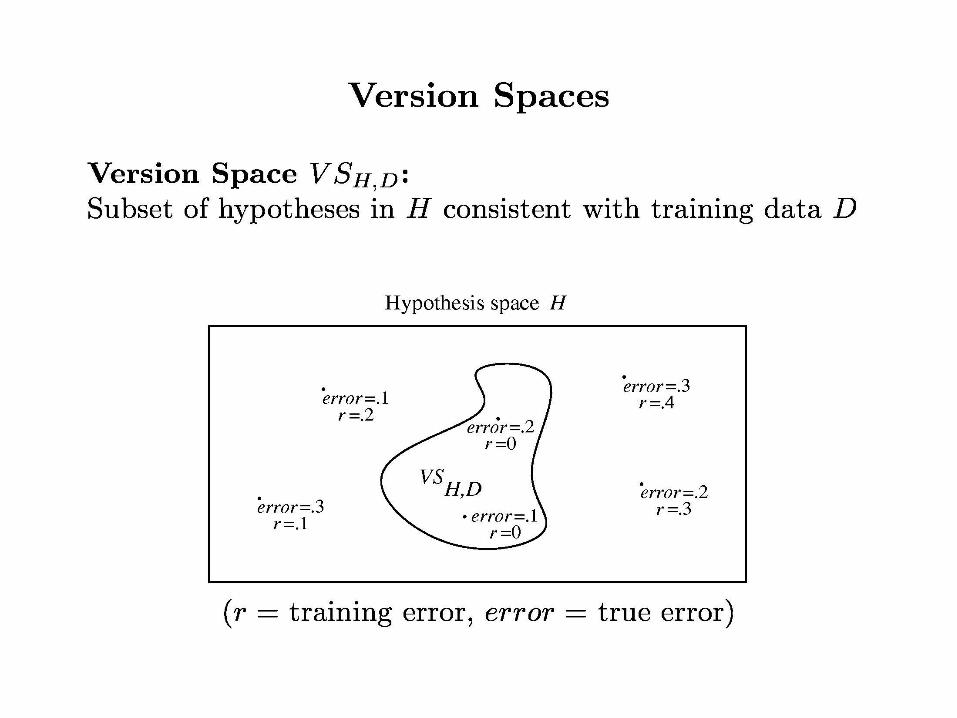
• By definition, a consistent learner must produce a hypothesis in the version space for H given D.
• Therefore, to bound the number of examples needed by a consistent learner, we just need to bound the number of examples needed to ensure that the version-space contains no hypotheses with unacceptably high error.
18
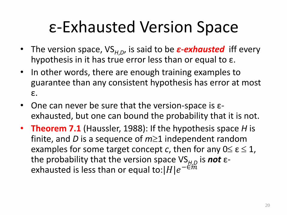
ε-Exhausted Version Space • The version space, VSH,D, is said to be ε-exhausted iff every
hypothesis in it has true error less than or equal to ε.
• In other words, there are enough training examples to guarantee than any consistent hypothesis has error at most ε.
• One can never be sure that the version-space is ε-exhausted, but one can bound the probability that it is not.
• Theorem 7.1 (Haussler, 1988): If the hypothesis space H is finite, and D is a sequence of m1 independent random examples for some target concept c, then for any 0 ε 1, the probability that the version space VSH,D is not ε-exhausted is less than or equal to:|𝐻|𝑒−∈𝑚
20
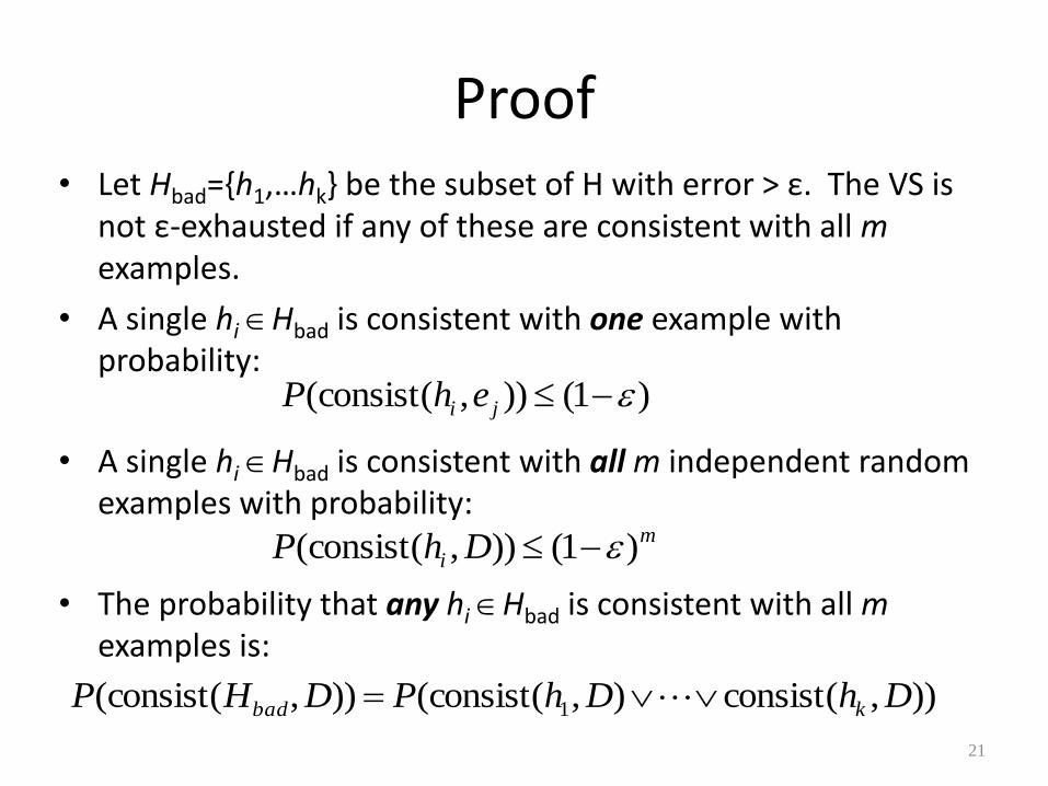
Proof • Let Hbad={h1,…hk} be the subset of H with error > ε. The VS is
not ε-exhausted if any of these are consistent with all m examples.
• A single hi Hbad is consistent with one example with probability:
• A single hi Hbad is consistent with all m independent random examples with probability:
• The probability that any hi Hbad is consistent with all m examples is:
21
)1()),(consist( ji ehP
m
i DhP )1()),(consist(
)),(consist),(consist()),(consist( 1 DhDhPDHP kbad
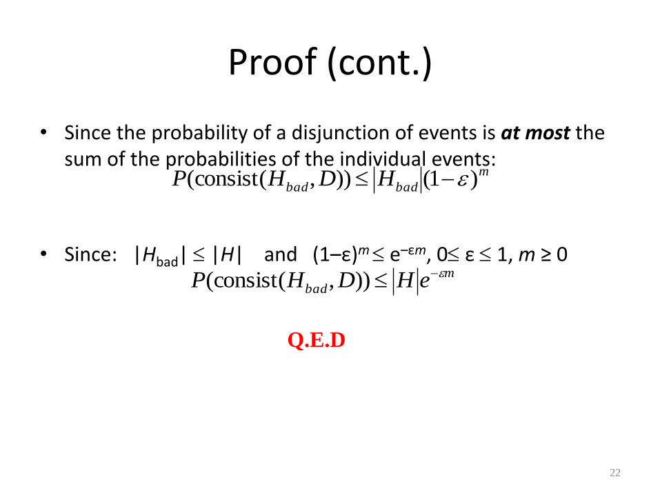
Proof (cont.)
• Since the probability of a disjunction of events is at most the sum of the probabilities of the individual events:
• Since: |Hbad| |H| and (1–ε)m e–εm, 0 ε 1, m ≥ 0
22
m
badbad HDHP )1()),(consist(
m
bad eHDHP )),(consist(
Q.E.D
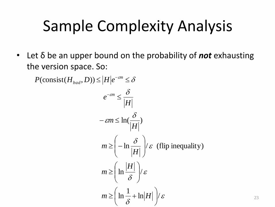
Sample Complexity Analysis
• Let δ be an upper bound on the probability of not exhausting the version space. So:
23
/ln1
ln
/ln
)inequality (flip /ln
)ln(
)),(consist(
Hm
Hm
Hm
Hm
He
eHDHP
m
m
bad
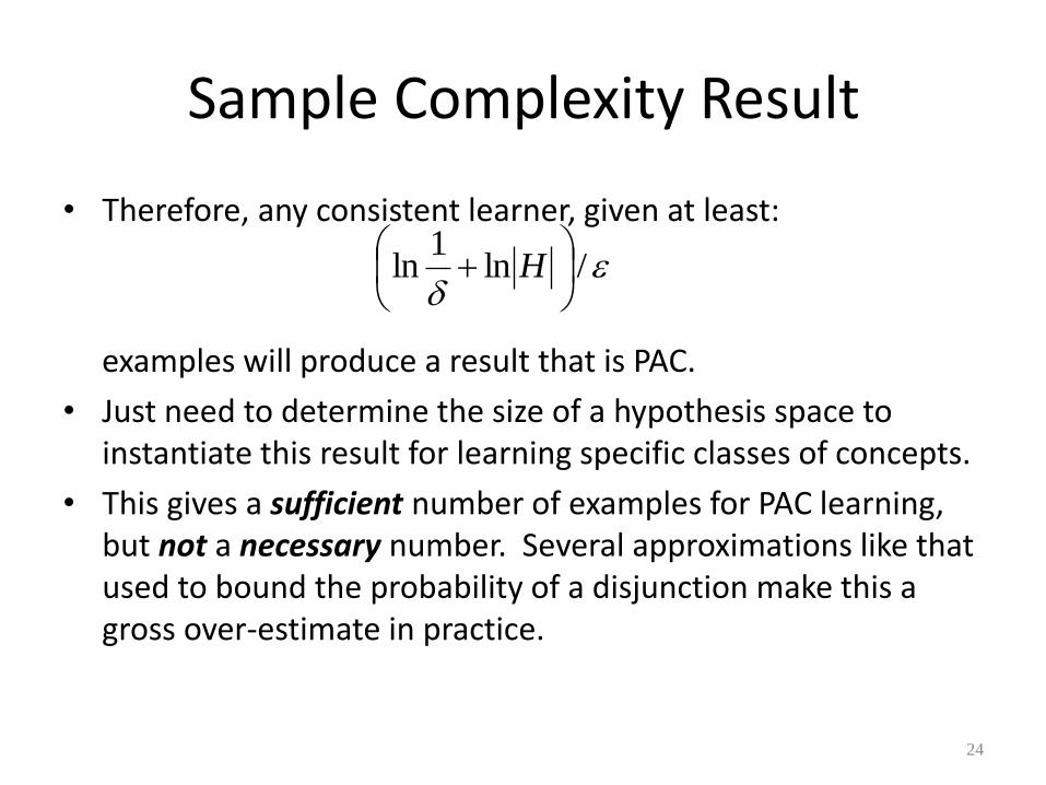
Sample Complexity Result
• Therefore, any consistent learner, given at least:
examples will produce a result that is PAC.
• Just need to determine the size of a hypothesis space to instantiate this result for learning specific classes of concepts.
• This gives a sufficient number of examples for PAC learning, but not a necessary number. Several approximations like that used to bound the probability of a disjunction make this a gross over-estimate in practice.
24
/ln1
ln
H
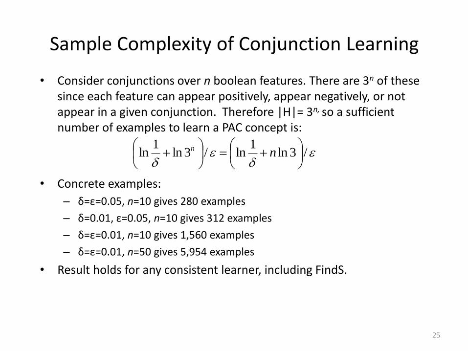
Sample Complexity of Conjunction Learning
• Consider conjunctions over n boolean features. There are 3n of these since each feature can appear positively, appear negatively, or not appear in a given conjunction. Therefore |H|= 3n, so a sufficient number of examples to learn a PAC concept is:
• Concrete examples:
– δ=ε=0.05, n=10 gives 280 examples
– δ=0.01, ε=0.05, n=10 gives 312 examples
– δ=ε=0.01, n=10 gives 1,560 examples
– δ=ε=0.01, n=50 gives 5,954 examples
• Result holds for any consistent learner, including FindS.
25
/3ln1
ln/3ln1
ln
nn
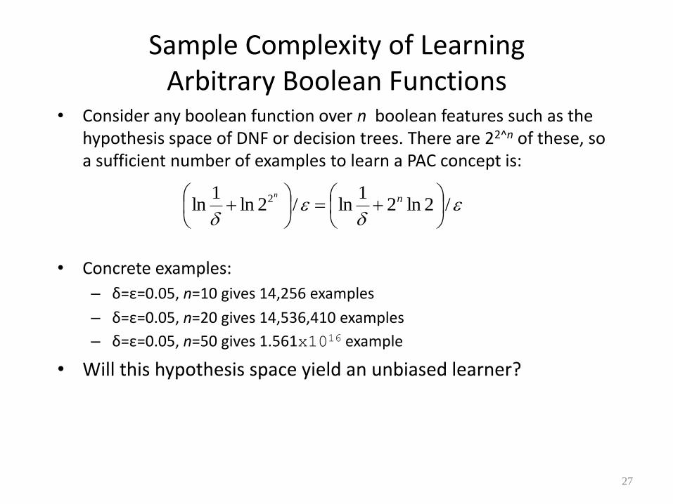
Sample Complexity of Learning Arbitrary Boolean Functions
• Consider any boolean function over n boolean features such as the hypothesis space of DNF or decision trees. There are 22^n of these, so a sufficient number of examples to learn a PAC concept is:
• Concrete examples:
– δ=ε=0.05, n=10 gives 14,256 examples
– δ=ε=0.05, n=20 gives 14,536,410 examples
– δ=ε=0.05, n=50 gives 1.561x10¹⁶ example
• Will this hypothesis space yield an unbiased learner?
27
/2ln21
ln/2ln1
ln 2
nn
Infinite Hypothesis Spaces
• The preceding analysis was restricted to finite hypothesis spaces. Moreover, the bounds were quite weak.
• Some infinite hypothesis spaces (such as those including real-valued thresholds or parameters) are more expressive than others. – Compare a rule allowing one threshold on a continuous feature
(length<3cm) vs one allowing two thresholds (1cm<length<3cm).
• Need some measure of the expressiveness of infinite hypothesis spaces.
• The Vapnik-Chervonenkis (VC) dimension provides just such a measure, denoted VC(H).
• Analogous to ln|H|, there are bounds for sample complexity using VC(H).
34
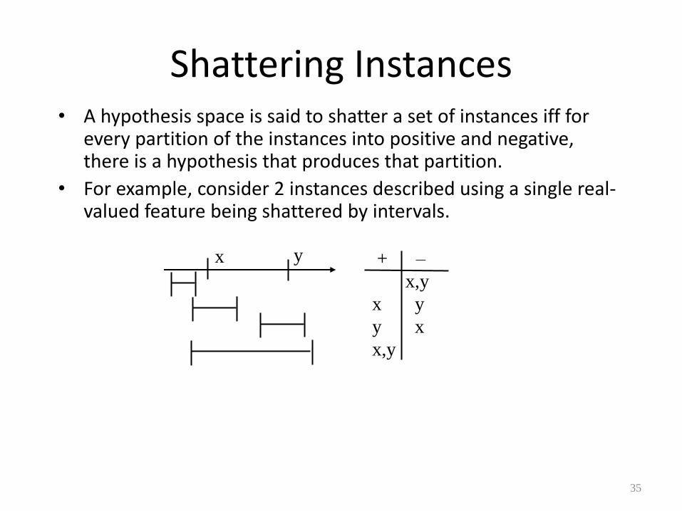
Shattering Instances • A hypothesis space is said to shatter a set of instances iff for
every partition of the instances into positive and negative, there is a hypothesis that produces that partition.
• For example, consider 2 instances described using a single real-valued feature being shattered by intervals.
35
+ –
_ x,y
x y
y x
x,y
x y
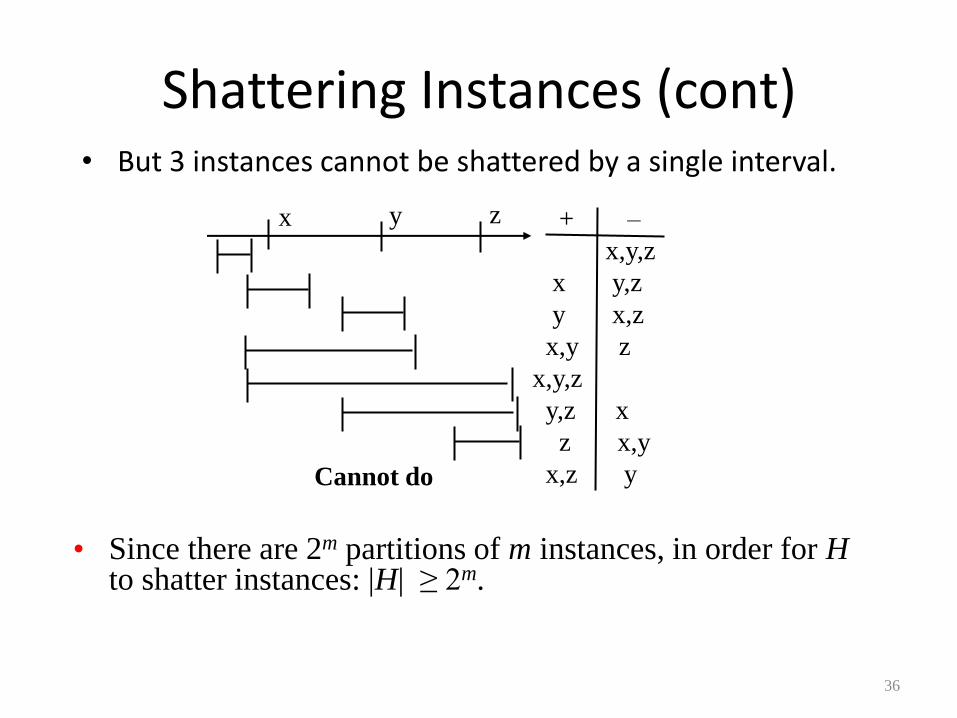
Shattering Instances (cont) • But 3 instances cannot be shattered by a single interval.
36
+ –
_ x,y,z
x y,z
y x,z
x,y z
x,y,z
y,z x
z x,y
x,z y
x y z
Cannot do
• Since there are 2m partitions of m instances, in order for H to shatter instances: |H| ≥ 2m.
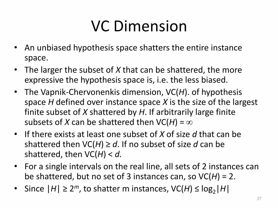
VC Dimension • An unbiased hypothesis space shatters the entire instance
space.
• The larger the subset of X that can be shattered, the more expressive the hypothesis space is, i.e. the less biased.
• The Vapnik-Chervonenkis dimension, VC(H). of hypothesis space H defined over instance space X is the size of the largest finite subset of X shattered by H. If arbitrarily large finite subsets of X can be shattered then VC(H) =
• If there exists at least one subset of X of size d that can be shattered then VC(H) ≥ d. If no subset of size d can be shattered, then VC(H) < d.
• For a single intervals on the real line, all sets of 2 instances can be shattered, but no set of 3 instances can, so VC(H) = 2.
• Since |H| ≥ 2m, to shatter m instances, VC(H) ≤ log2|H| 37
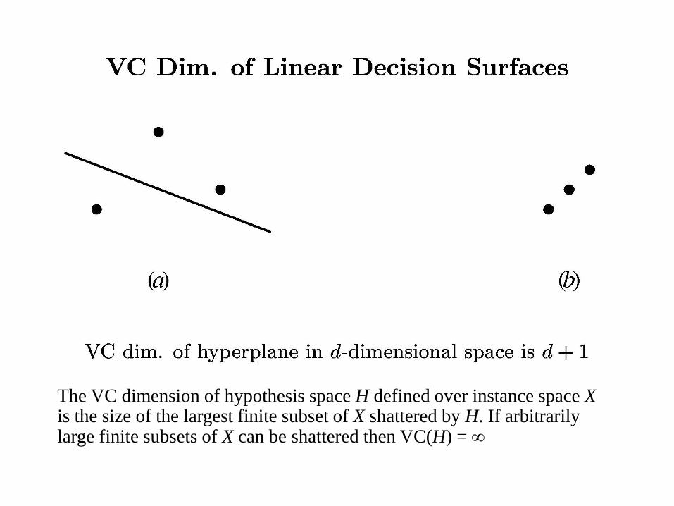
The VC dimension of hypothesis space H defined over instance space X is the size of the largest finite subset of X shattered by H. If arbitrarily large finite subsets of X can be shattered then VC(H) =
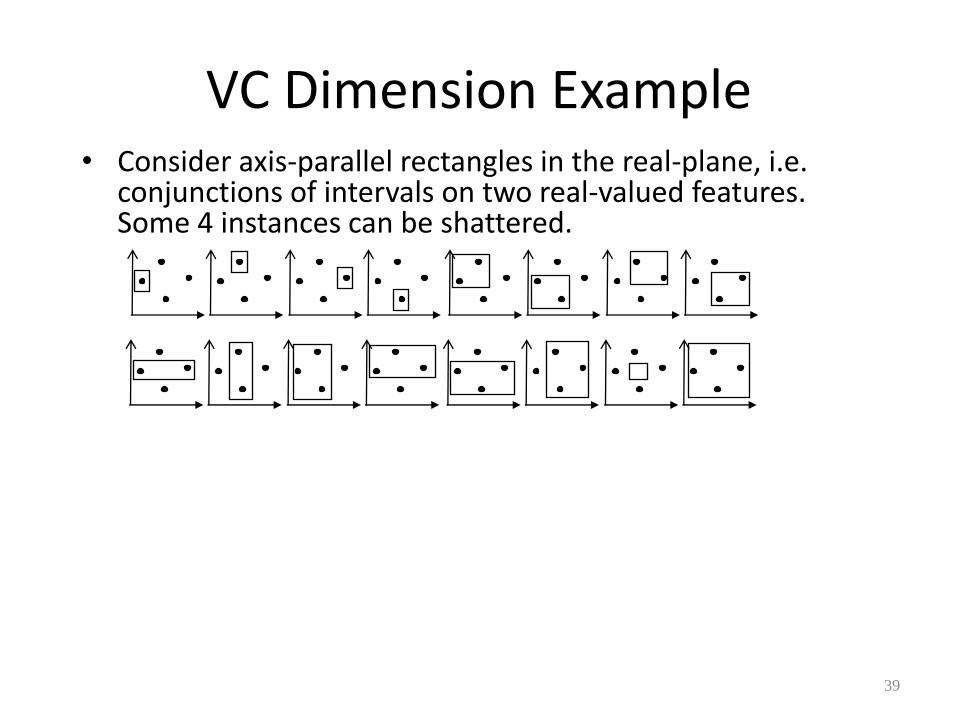
VC Dimension Example • Consider axis-parallel rectangles in the real-plane, i.e.
conjunctions of intervals on two real-valued features. Some 4 instances can be shattered.
39
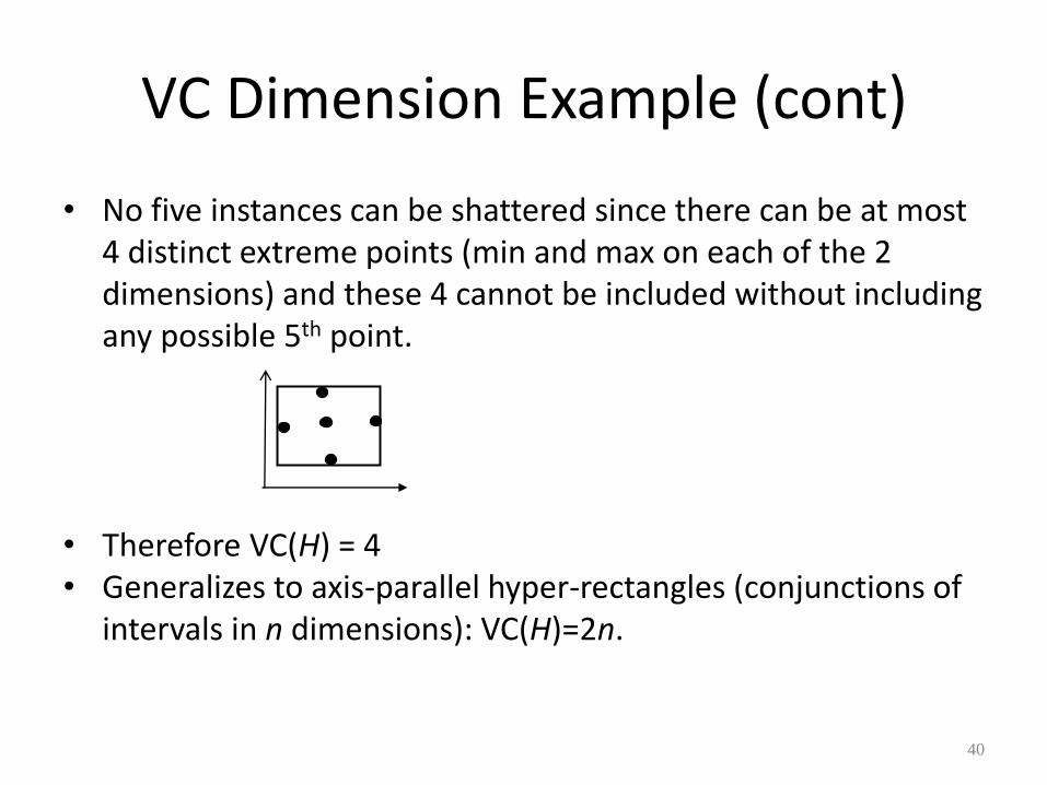
VC Dimension Example (cont)
• No five instances can be shattered since there can be at most 4 distinct extreme points (min and max on each of the 2 dimensions) and these 4 cannot be included without including any possible 5th point.
• Therefore VC(H) = 4 • Generalizes to axis-parallel hyper-rectangles (conjunctions of
intervals in n dimensions): VC(H)=2n.
40
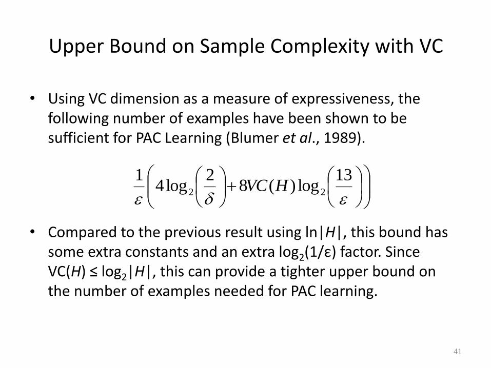
Upper Bound on Sample Complexity with VC
• Using VC dimension as a measure of expressiveness, the following number of examples have been shown to be sufficient for PAC Learning (Blumer et al., 1989).
• Compared to the previous result using ln|H|, this bound has some extra constants and an extra log2(1/ε) factor. Since VC(H) ≤ log2|H|, this can provide a tighter upper bound on the number of examples needed for PAC learning.
41
13log)(8
2log4
122 HVC
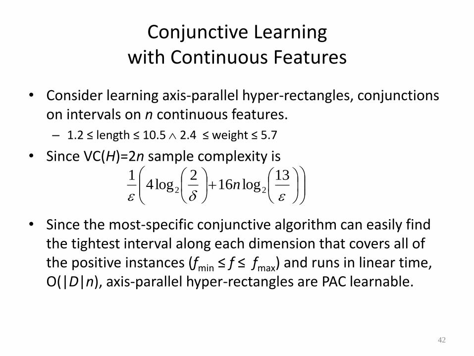
Conjunctive Learning with Continuous Features
• Consider learning axis-parallel hyper-rectangles, conjunctions on intervals on n continuous features.
– 1.2 ≤ length ≤ 10.5 2.4 ≤ weight ≤ 5.7
• Since VC(H)=2n sample complexity is
• Since the most-specific conjunctive algorithm can easily find the tightest interval along each dimension that covers all of the positive instances (fmin ≤ f ≤ fmax) and runs in linear time, O(|D|n), axis-parallel hyper-rectangles are PAC learnable.
42
13log16
2log4
122 n
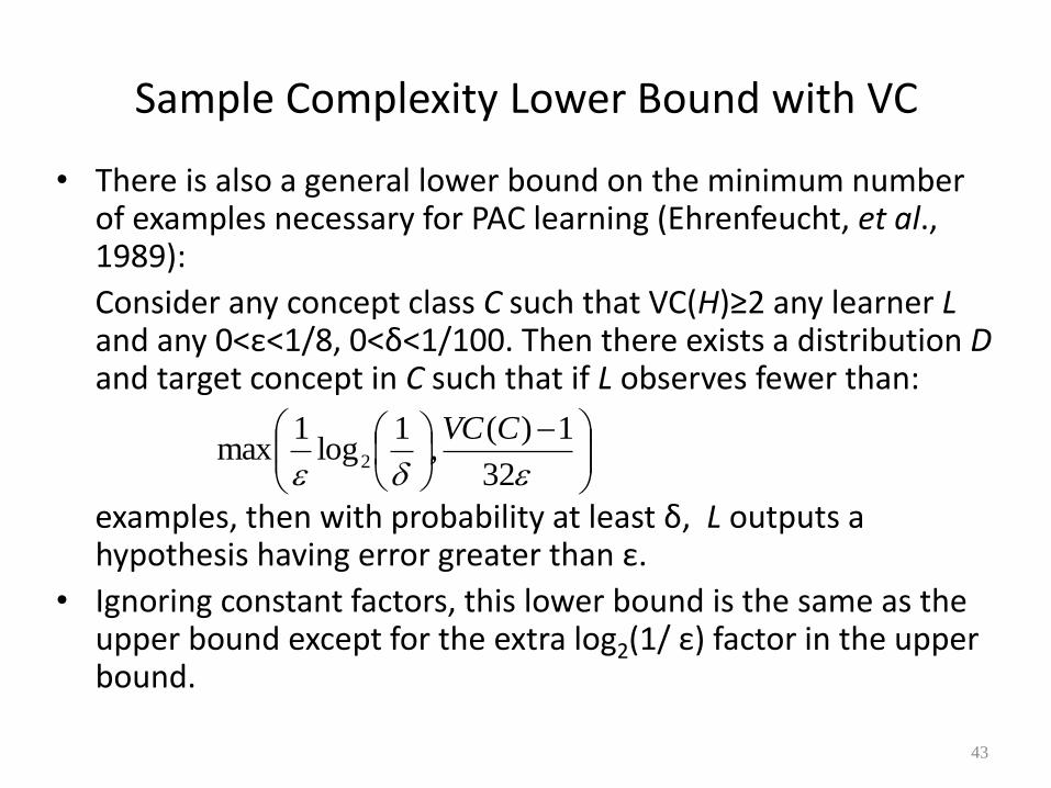
Sample Complexity Lower Bound with VC
• There is also a general lower bound on the minimum number of examples necessary for PAC learning (Ehrenfeucht, et al., 1989):
Consider any concept class C such that VC(H)≥2 any learner L and any 0<ε<1/8, 0<δ<1/100. Then there exists a distribution D and target concept in C such that if L observes fewer than:
examples, then with probability at least δ, L outputs a hypothesis having error greater than ε.
• Ignoring constant factors, this lower bound is the same as the upper bound except for the extra log2(1/ ε) factor in the upper bound.
43
32
1)(,
1log
1max 2
CVC
No Free Lunch Theorem
• If we are interested solely in the generalization performance, are there any reasons to prefer one classifier over the other?
• If we make no prior assumptions about the nature of the classification task, can we expect any classification method to be superior overall?
• Can we find an algorithm that is superior to random guessing?
• Answer is No
48
Implications of No free Lunch theorem
• No context-independent or usage-independent reasons to prefer one classifier over the other
• If one algorithm seems to outperform another in a particular situation, it is a consequence of its (over??)fit to the particular domain – Does not imply general superiority
• In practice what matters most is – Prior knowledge – Data distribution – Amount of training data
• Try different approaches and compare • Off-training-set error: The test-set should be such that it
contains no examples that are in the training set
49
No Free Lunch, Overfitting Avoidance and Occam’s Razro
• We saw how to avoid overfitting
– Regularization, pruning, inclusion of penalty, etc.
• Occam’s razor: one should not use classifiers that are more complicated than necessary
• No free lunch invalidates these techniques
– If there is no reason to prefer one over the other why are overfitting techniques and simpler models universally advocated
50
So Why are these techniques successful?
• Classes of problems addressed so far have certain properties
• Evolution: we have a strong selection pressure to be computationally simple.
• Satisficing (Herb Simon): Creating an adequate though possibly non-optimal solution
– Underlying much of machine learning and human cognition
51
COLT Conclusions • The PAC framework provides a theoretical framework for
analyzing the effectiveness of learning algorithms. • The sample complexity for any consistent learner using
some hypothesis space, H, can be determined from a measure of its expressiveness |H| or VC(H), quantifying bias and relating it to generalization.
• If sample complexity is tractable, then the computational complexity of finding a consistent hypothesis in H governs its PAC learnability.
• Constant factors are more important in sample complexity than in computational complexity, since our ability to gather data is generally not growing exponentially.
• Experimental results suggest that theoretical sample complexity bounds over-estimate the number of training instances needed in practice since they are worst-case upper bounds.
52