CS 6293 Advanced Topics: Current Bioinformatics

Motif finding

HW2

• Available on course website• First part: theoretical questions. Due on Mon, Oct 25• Second part: Presentation on Mon, Nov 1• Bonus: email me who are in your group and the papers

you choose, by Wed, Oct 20.• 7 minutes presentation + 2 minutes Q&A

– You can choose to go to some really cool details or give the main ideas of the papers

• Group size 1 or 2 acceptable, with the same expectation

• Last slide of presentation– Contributions from group members

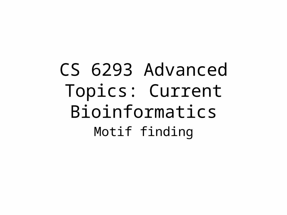
What is a (biological) motif?

• A motif is a recurring fragment, theme or pattern• Sequence motif: a sequence pattern of nucleotides in a

DNA sequence or amino acids in a protein • Structural motif: a pattern in a protein structure formed

by the spatial arrangement of amino acids.• Network motif: patterns that occur in different parts of a

network at frequencies much higher than those found in randomized network

• Commonality: – higher frequency than would be expected by chance– Has, or is conjectured to have, a biological significance

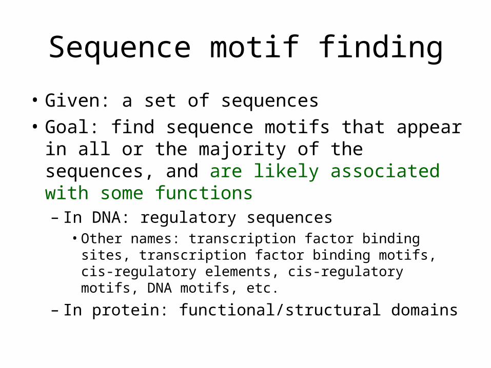
Sequence motif finding

• Given: a set of sequences

• Goal: find sequence motifs that appear in all or the majority of the sequences, and are likely associated with some functions– In DNA: regulatory sequences

• Other names: transcription factor binding sites, transcription factor binding motifs, cis-regulatory elements, cis-regulatory motifs, DNA motifs, etc.

– In protein: functional/structural domains

Roadmap

• Biological background

• Representation of motifs

• Algorithms for finding motifs

• Other issues– Search for instances of given motifs– Distinguish functional vs non-functional motifs

Biological background for motif finding

Genome is fixed – Cells are dynamic

• A genome is static– (almost) Every cell in our body has a copy of

the same genome

• A cell is dynamic– Responds to internal/external conditions– Most cells follow a cell cycle of division– Cells differentiate during development

Gene regulation

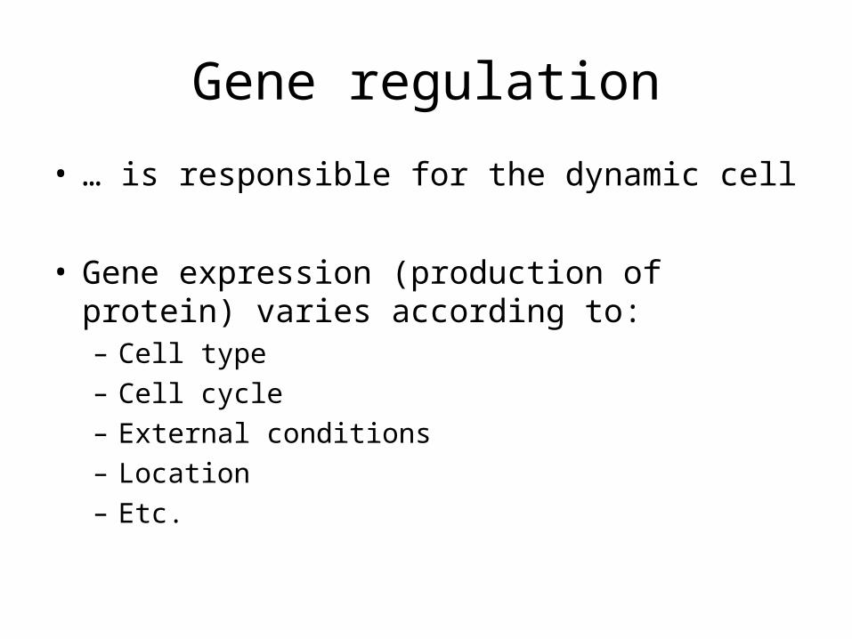
• … is responsible for the dynamic cell

• Gene expression (production of protein) varies according to:– Cell type– Cell cycle– External conditions– Location– Etc.

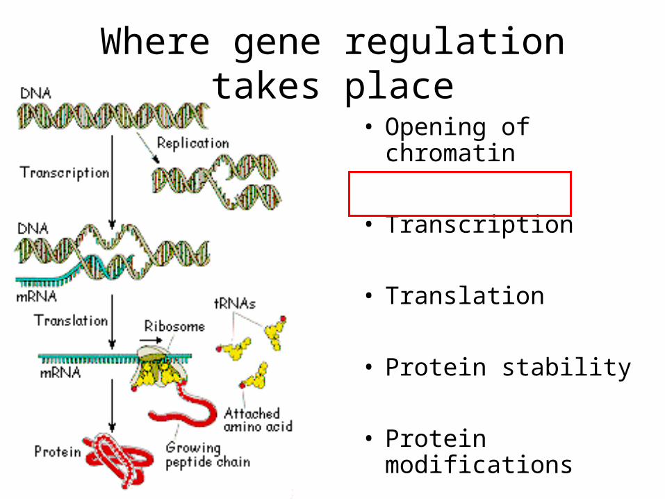
Where gene regulation takes place

• Opening of chromatin

• Transcription

• Translation

• Protein stability

• Protein modifications

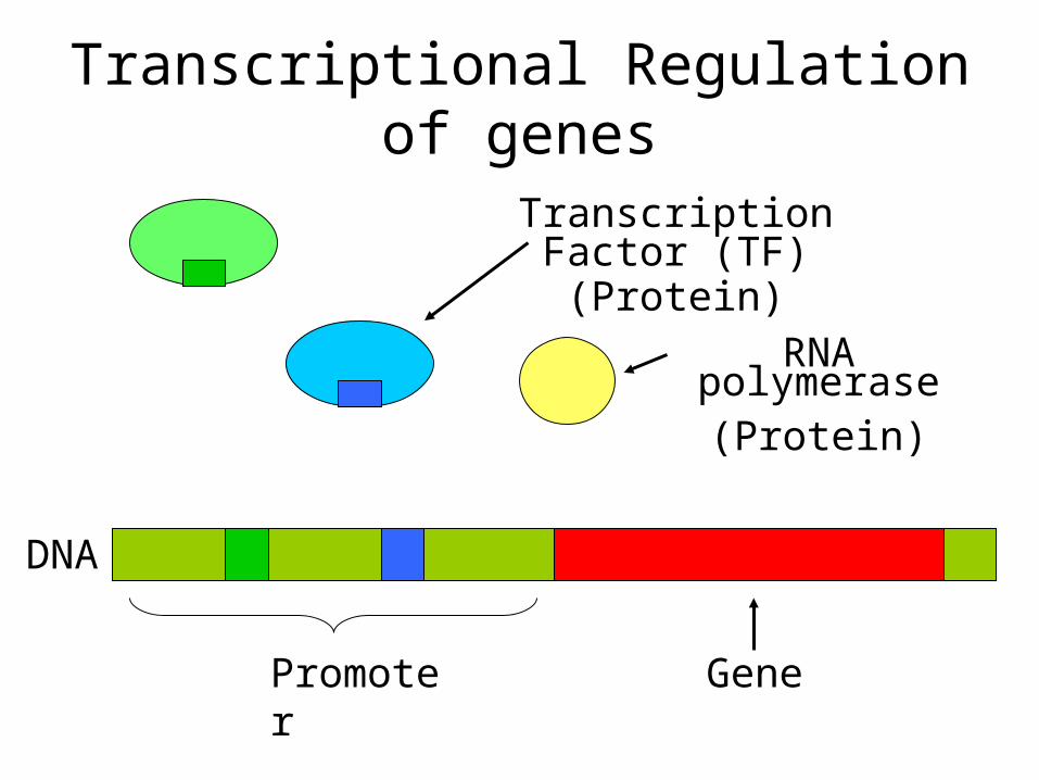
GenePromoter

RNA polymerase(Protein)

Transcription Factor (TF)(Protein)

DNA

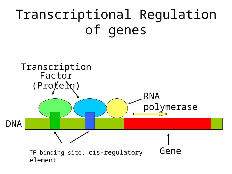
Transcriptional Regulation of genes

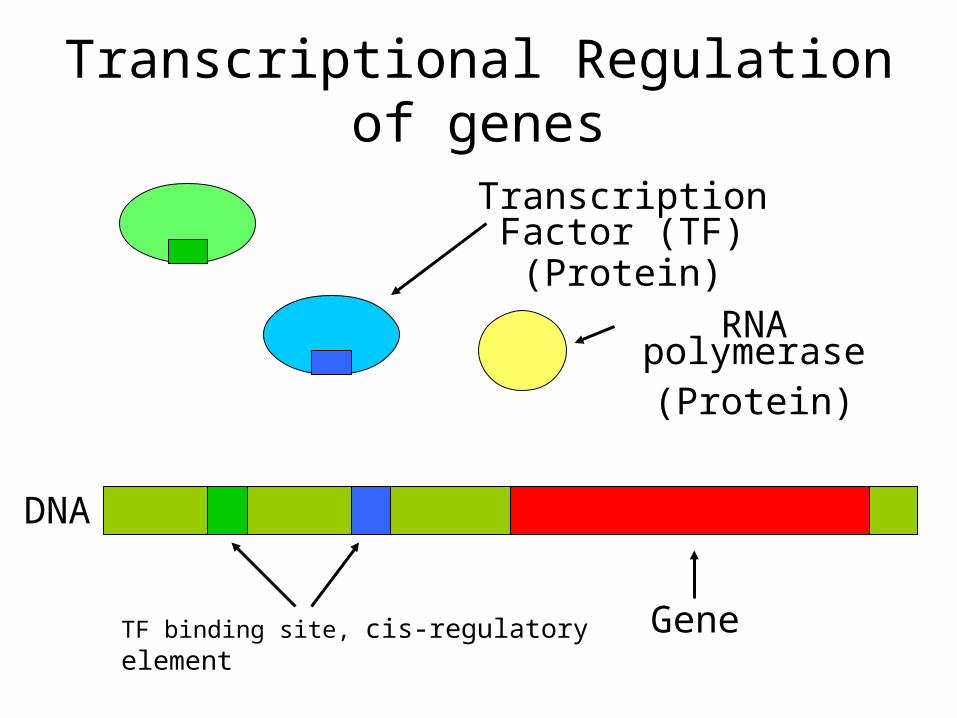
GeneTF binding site, cis-regulatory element

RNA polymerase(Protein)

Transcription Factor (TF)(Protein)

DNA

Transcriptional Regulation of genes

Transcriptional Regulation of genes

Gene

RNA polymerase

Transcription Factor(Protein)

DNA

TF binding site, cis-regulatory element

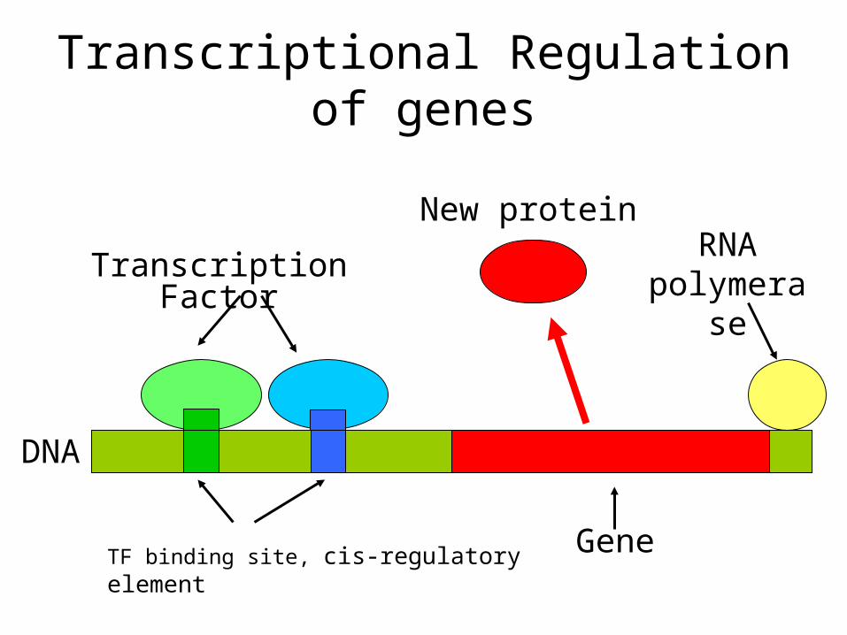
Gene

RNA polymerase

Transcription Factor

DNA

New protein

Transcriptional Regulation of genes

TF binding site, cis-regulatory element

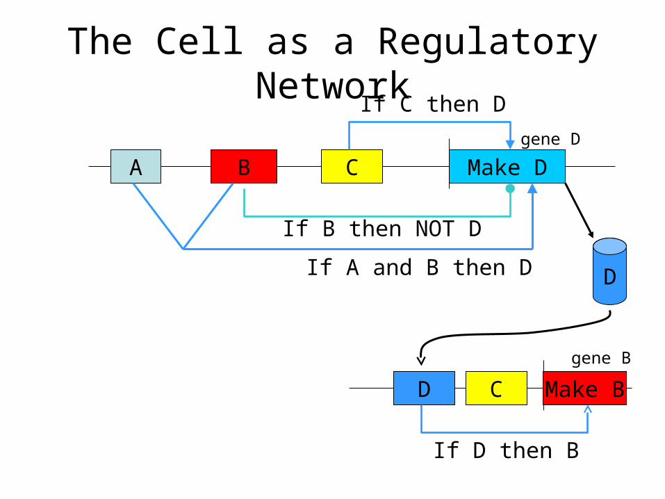
The Cell as a Regulatory Network

A B Make DC

If C then D

If B then NOT D

If A and B then D D

Make BD

If D then B

C

gene D

gene B

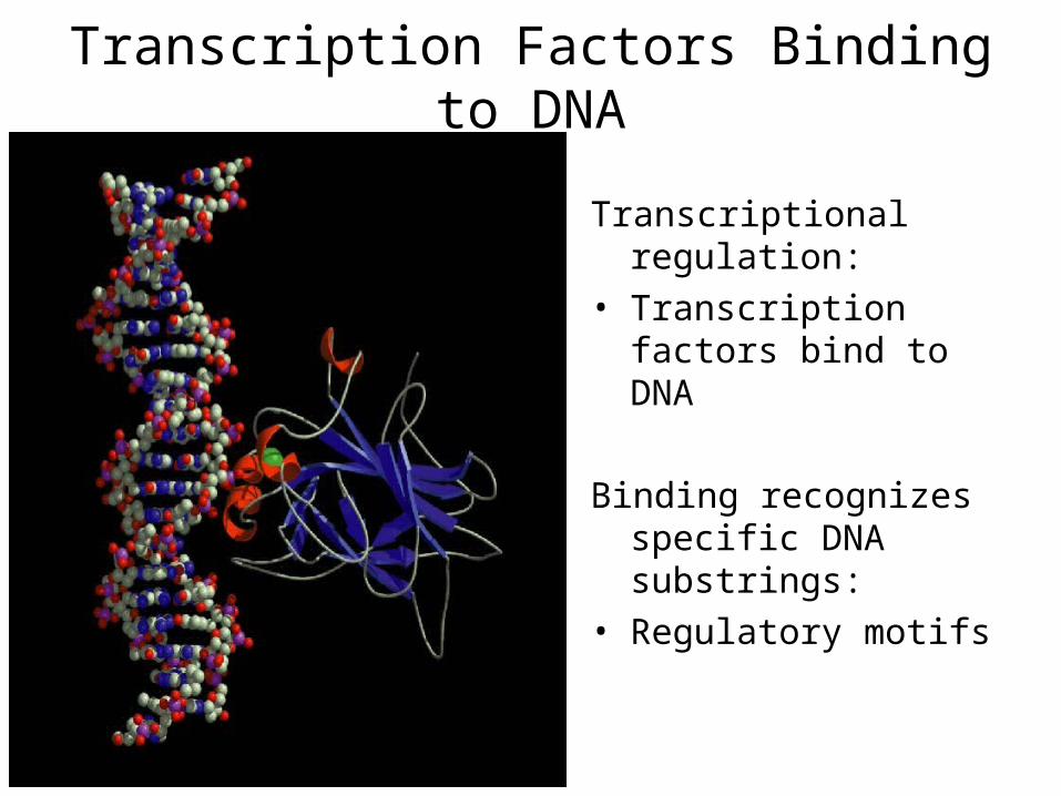
Transcription Factors Binding to DNA

Transcriptional regulation:• Transcription factors

bind to DNA

Binding recognizes specific DNA substrings:

• Regulatory motifs

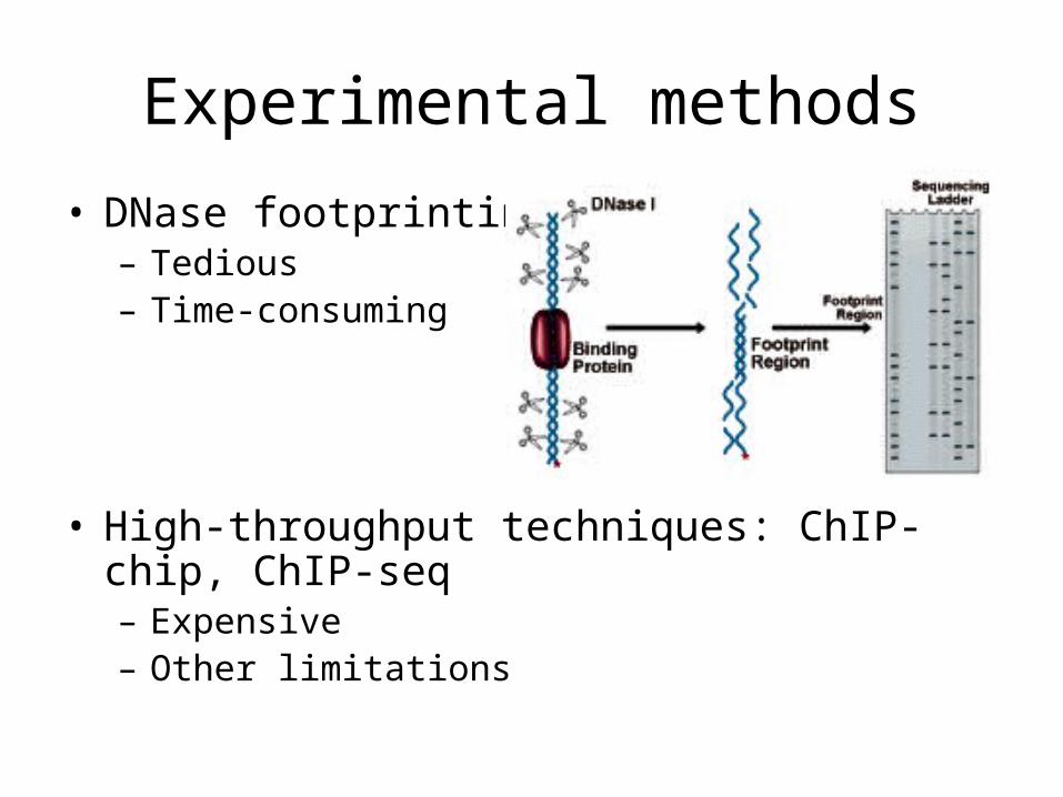
Experimental methods

• DNase footprinting– Tedious – Time-consuming

• High-throughput techniques: ChIP-chip, ChIP-seq– Expensive– Other limitations

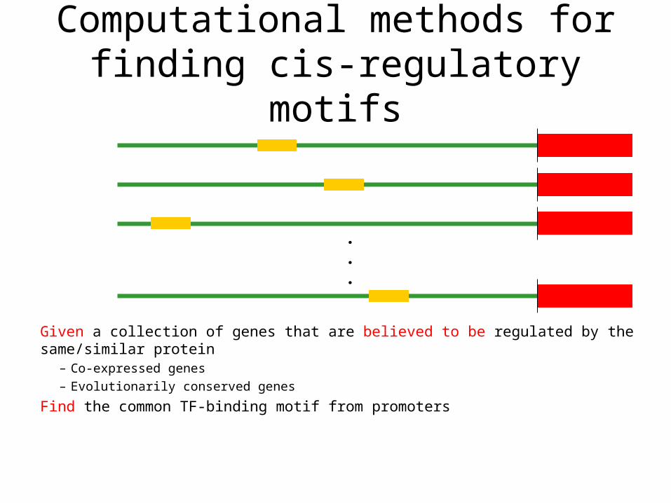
Computational methods for finding cis-regulatory motifs

Given a collection of genes that are believed to be regulated by the same/similar protein– Co-expressed genes– Evolutionarily conserved genes

Find the common TF-binding motif from promoters

.

.

.

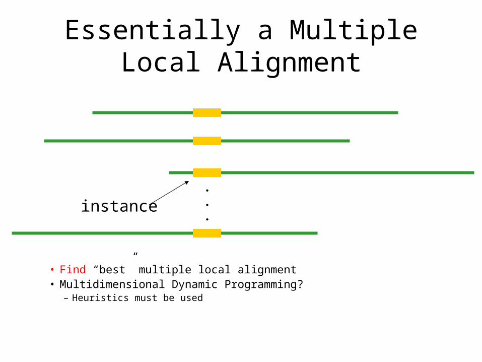
Essentially a Multiple Local Alignment

• Find “best” multiple local alignment• Multidimensional Dynamic Programming?

– Heuristics must be used

.

.

.instance

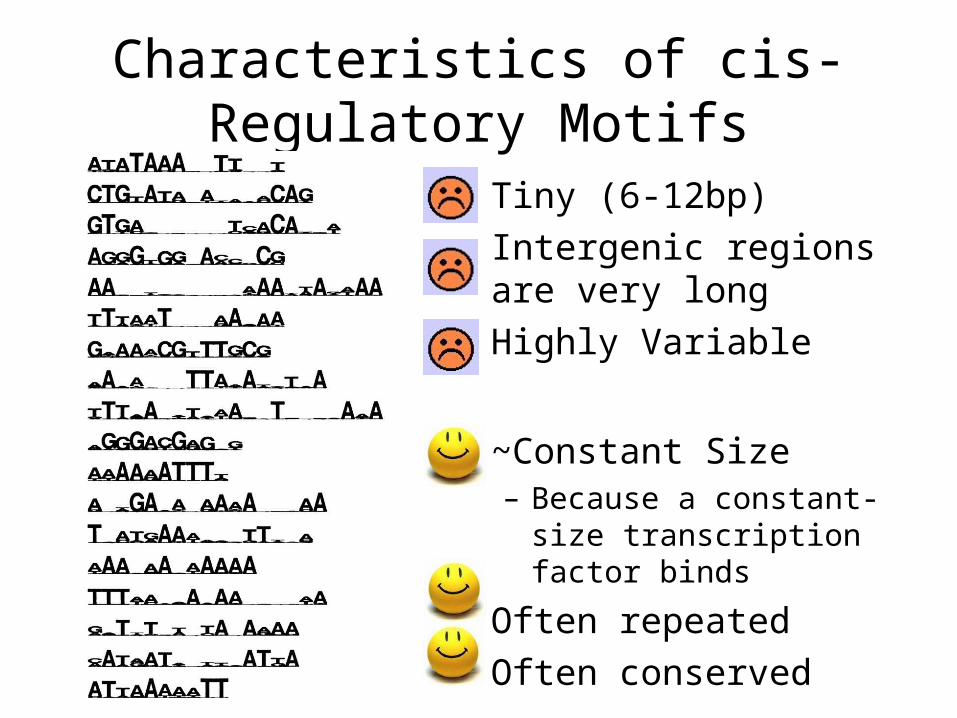
Characteristics of cis-Regulatory Motifs

• Tiny (6-12bp)• Intergenic regions are

very long • Highly Variable

• ~Constant Size– Because a constant-size

transcription factor binds

• Often repeated• Often conserved

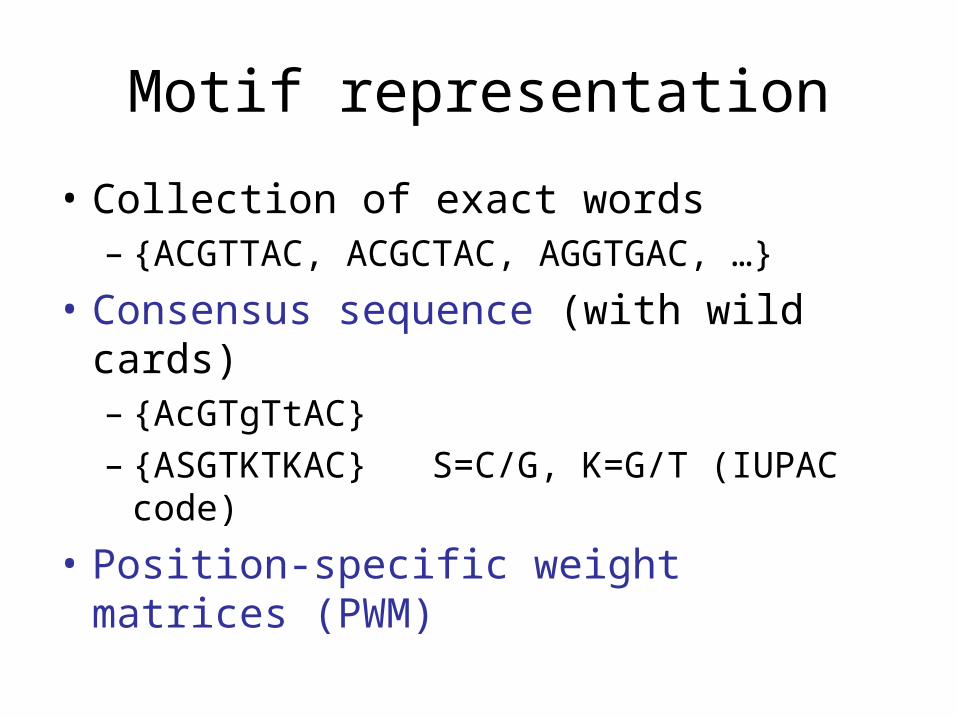
Motif representation

• Collection of exact words– {ACGTTAC, ACGCTAC, AGGTGAC, …}

• Consensus sequence (with wild cards)– {AcGTgTtAC}– {ASGTKTKAC} S=C/G, K=G/T (IUPAC code)

• Position-specific weight matrices (PWM)

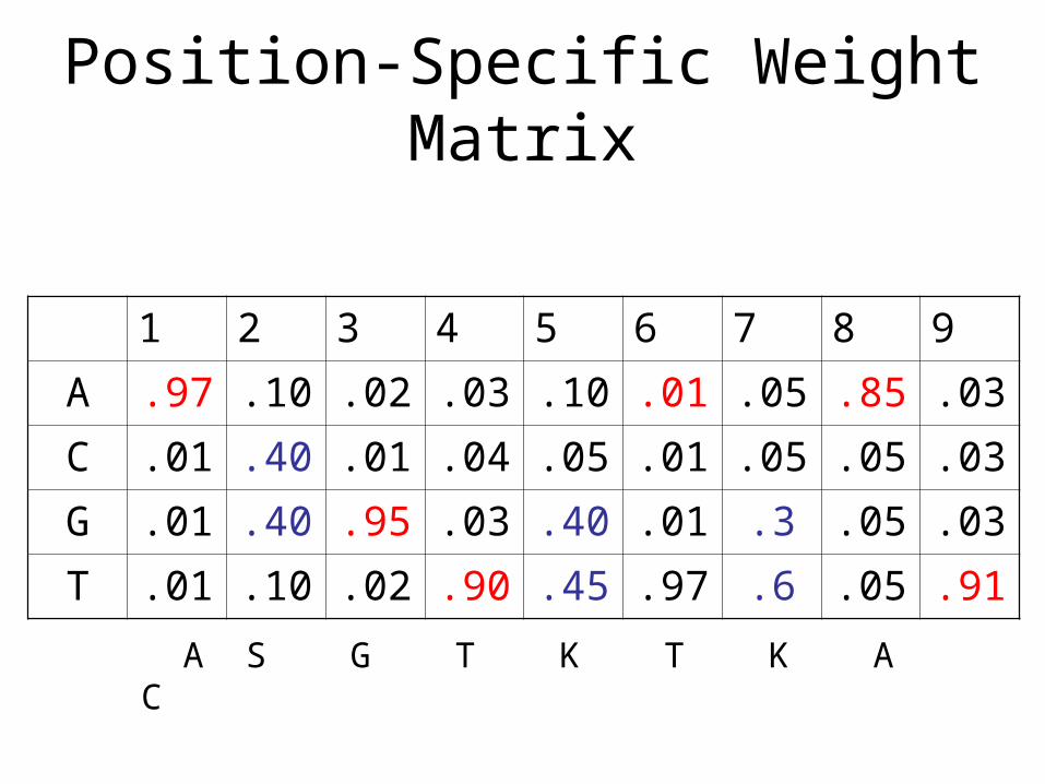
Position-Specific Weight Matrix

1 2 3 4 5 6 7 8 9

A .97 .10 .02 .03 .10 .01 .05 .85 .03

C .01 .40 .01 .04 .05 .01 .05 .05 .03

G .01 .40 .95 .03 .40 .01 .3 .05 .03

T .01 .10 .02 .90 .45 .97 .6 .05 .91

A S G T K T K A C

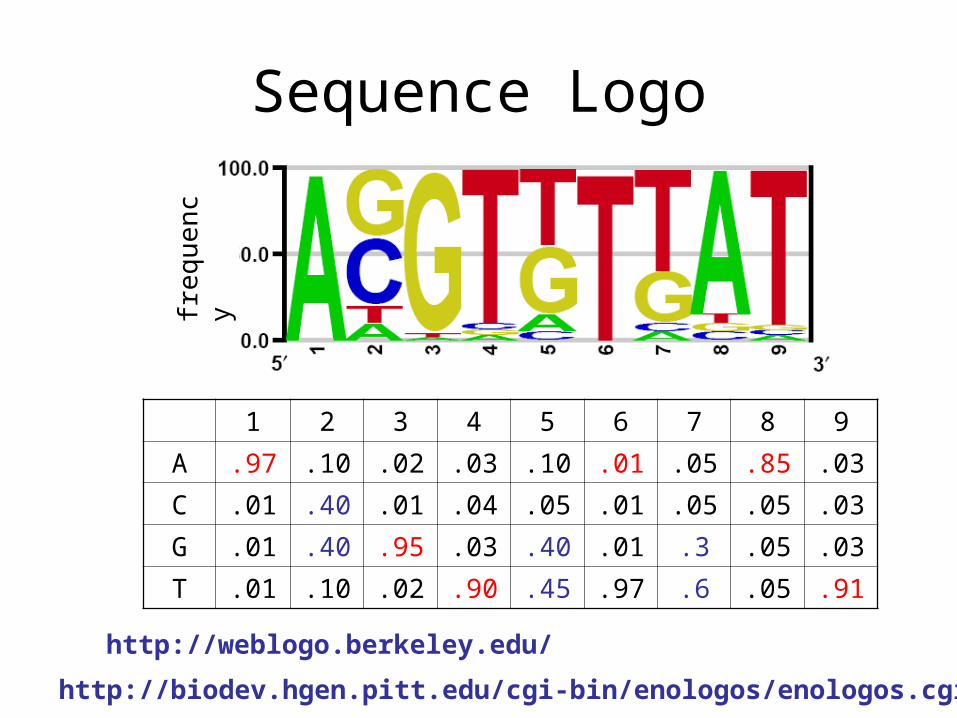
Sequence Logo

fre

que

ncy

1 2 3 4 5 6 7 8 9

A .97 .10 .02 .03 .10 .01 .05 .85 .03

C .01 .40 .01 .04 .05 .01 .05 .05 .03

G .01 .40 .95 .03 .40 .01 .3 .05 .03

T .01 .10 .02 .90 .45 .97 .6 .05 .91

http://weblogo.berkeley.edu/

http://biodev.hgen.pitt.edu/cgi-bin/enologos/enologos.cgi

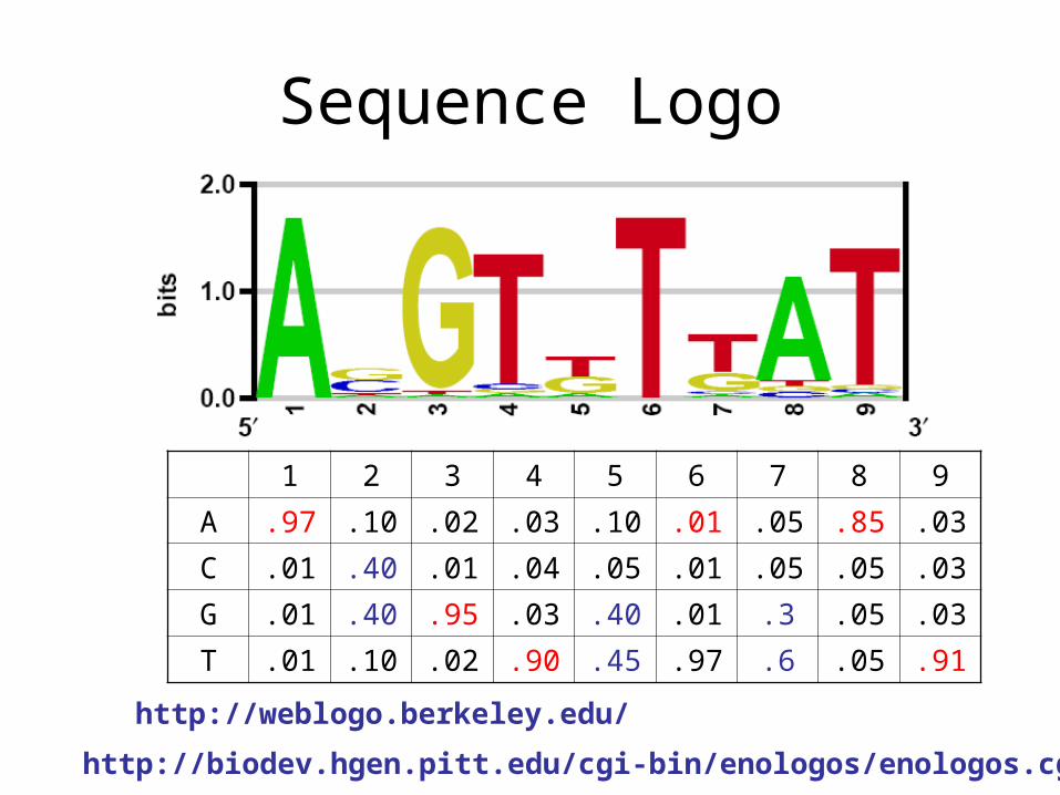
Sequence Logo

1 2 3 4 5 6 7 8 9

A .97 .10 .02 .03 .10 .01 .05 .85 .03

C .01 .40 .01 .04 .05 .01 .05 .05 .03

G .01 .40 .95 .03 .40 .01 .3 .05 .03

T .01 .10 .02 .90 .45 .97 .6 .05 .91

http://weblogo.berkeley.edu/

http://biodev.hgen.pitt.edu/cgi-bin/enologos/enologos.cgi

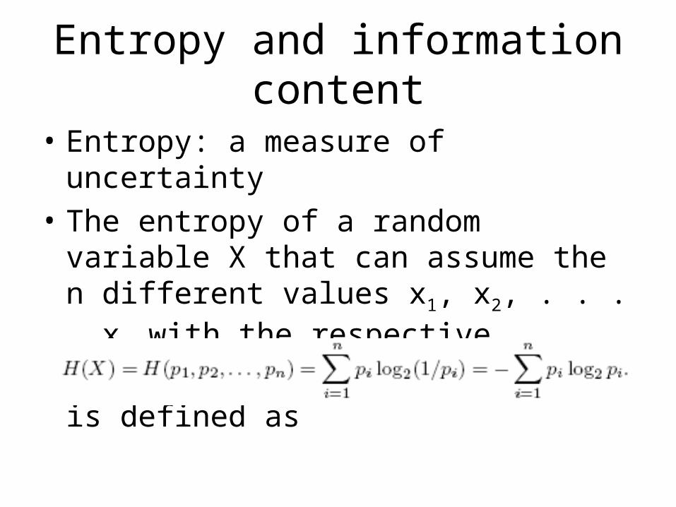
Entropy and information content

• Entropy: a measure of uncertainty

• The entropy of a random variable X that can assume the n different values x1, x2, . . . , xn with the respective probabilities p1, p2, . . . , pn is defined as

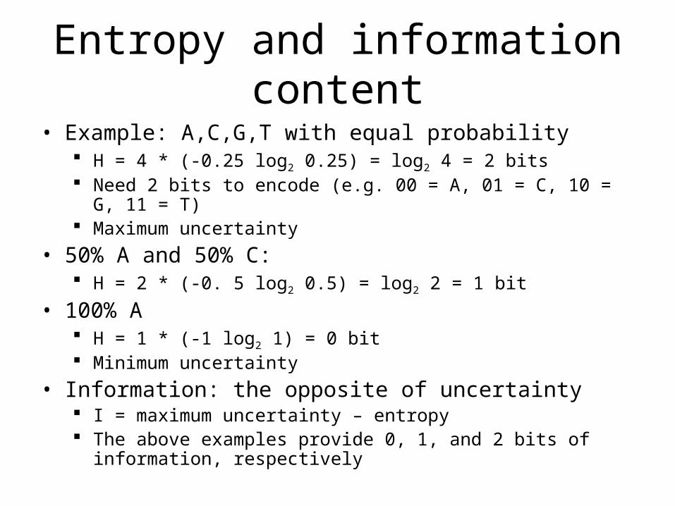
Entropy and information content

• Example: A,C,G,T with equal probability H = 4 * (-0.25 log2 0.25) = log2 4 = 2 bits Need 2 bits to encode (e.g. 00 = A, 01 = C, 10 = G, 11 = T) Maximum uncertainty

• 50% A and 50% C: H = 2 * (-0. 5 log2 0.5) = log2 2 = 1 bit

• 100% A H = 1 * (-1 log2 1) = 0 bit Minimum uncertainty

• Information: the opposite of uncertainty I = maximum uncertainty – entropy The above examples provide 0, 1, and 2 bits of information,

respectively

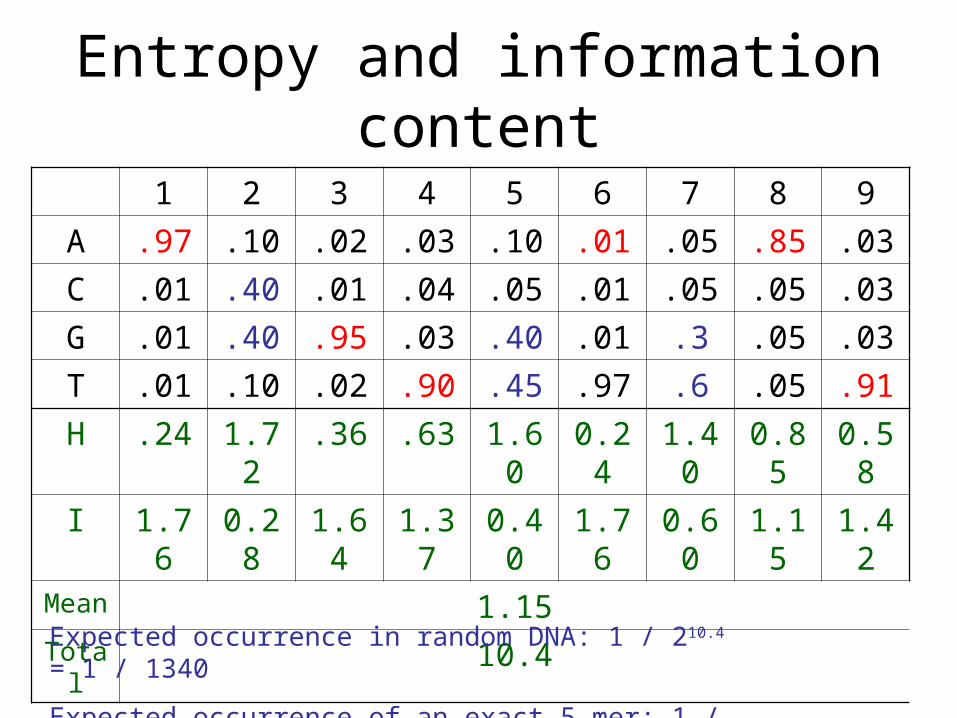
Entropy and information content

1 2 3 4 5 6 7 8 9

A .97 .10 .02 .03 .10 .01 .05 .85 .03

C .01 .40 .01 .04 .05 .01 .05 .05 .03

G .01 .40 .95 .03 .40 .01 .3 .05 .03

T .01 .10 .02 .90 .45 .97 .6 .05 .91

H .24 1.72 .36 .63 1.60 0.24 1.40 0.85 0.58

I 1.76 0.28 1.64 1.37 0.40 1.76 0.60 1.15 1.42Mean 1.15Total 10.4

Expected occurrence in random DNA: 1 / 210.4 = 1 / 1340

Expected occurrence of an exact 5-mer: 1 / 210 = 1 / 1024

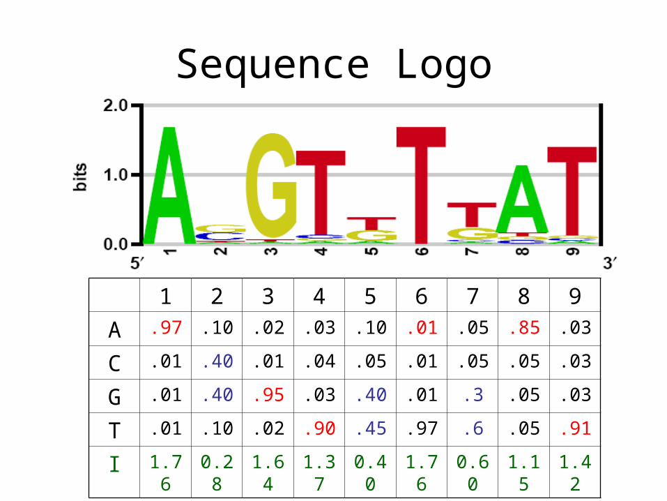
Sequence Logo

1 2 3 4 5 6 7 8 9

A .97 .10 .02 .03 .10 .01 .05 .85 .03

C .01 .40 .01 .04 .05 .01 .05 .05 .03

G .01 .40 .95 .03 .40 .01 .3 .05 .03

T .01 .10 .02 .90 .45 .97 .6 .05 .91

I 1.76 0.28 1.64 1.37 0.40 1.76 0.60 1.15 1.42

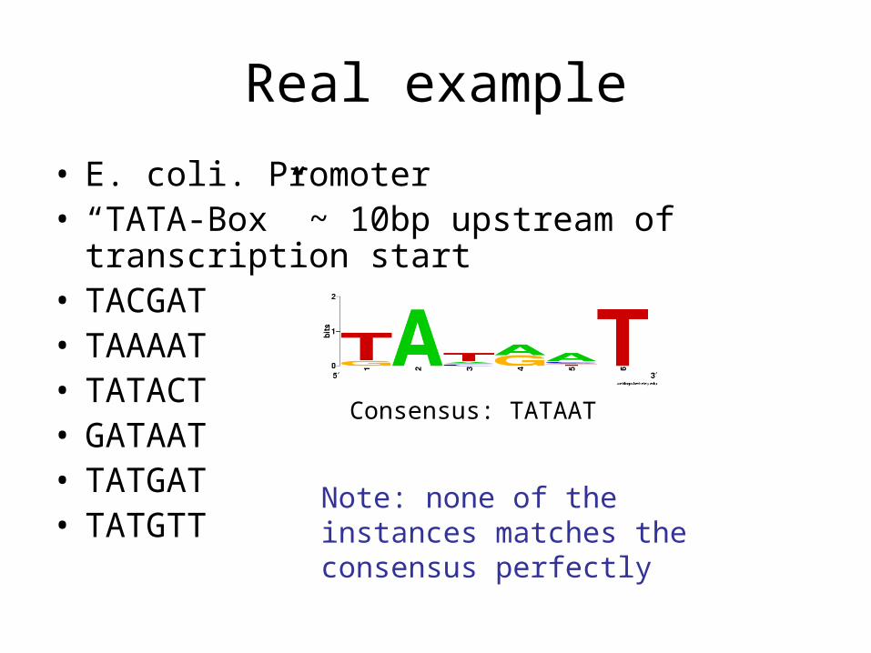
Real example

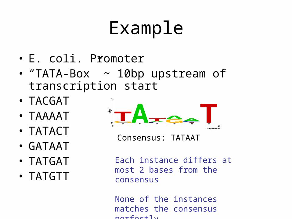
• E. coli. Promoter• “TATA-Box” ~ 10bp upstream of transcription

start• TACGAT• TAAAAT• TATACT• GATAAT• TATGAT• TATGTT

Consensus: TATAAT

Note: none of the instances matches the consensus perfectly

Finding Motifs

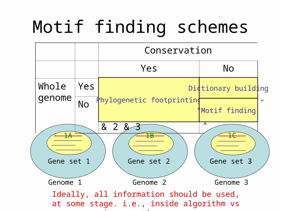
Motif finding schemes

Genome 1 Genome 2

Gene set 1 Gene set 2

Conservation

Yes No

Whole genome

Yes Genome 1 & 2 & 3 Genome 1

No Gene 1A & 1B & 1C or Gene Set 1 & 2 & 3

Gene Set 1

Genome 3

Gene set 3

1A 1B 1C

Phylogenetic footprinting

Dictionary building

“Motif finding”

Ideally, all information should be used, at some stage. i.e., inside algorithm vs pre- or post-processing.

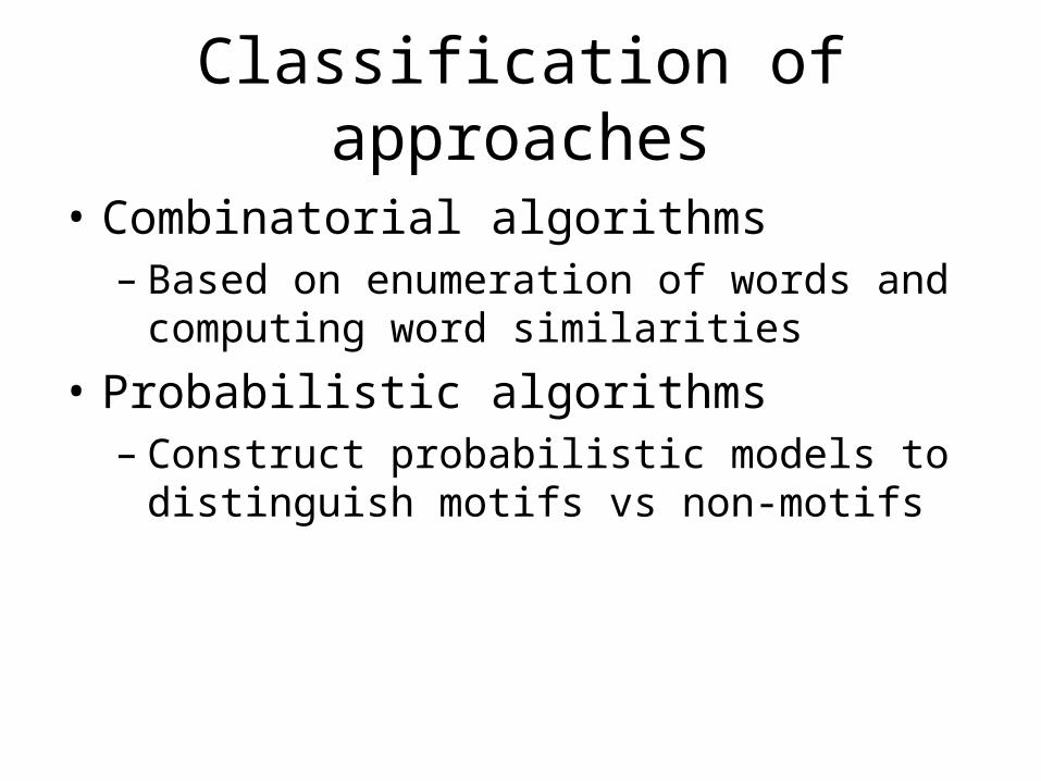
Classification of approaches

• Combinatorial algorithms– Based on enumeration of words and

computing word similarities

• Probabilistic algorithms– Construct probabilistic models to distinguish

motifs vs non-motifs

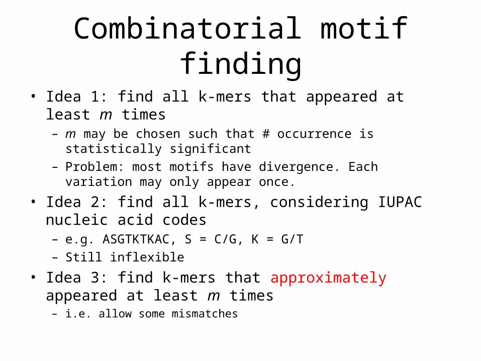
Combinatorial motif finding

• Idea 1: find all k-mers that appeared at least m times – m may be chosen such that # occurrence is statistically

significant– Problem: most motifs have divergence. Each variation may only

appear once.

• Idea 2: find all k-mers, considering IUPAC nucleic acid codes– e.g. ASGTKTKAC, S = C/G, K = G/T– Still inflexible

• Idea 3: find k-mers that approximately appeared at least m times– i.e. allow some mismatches

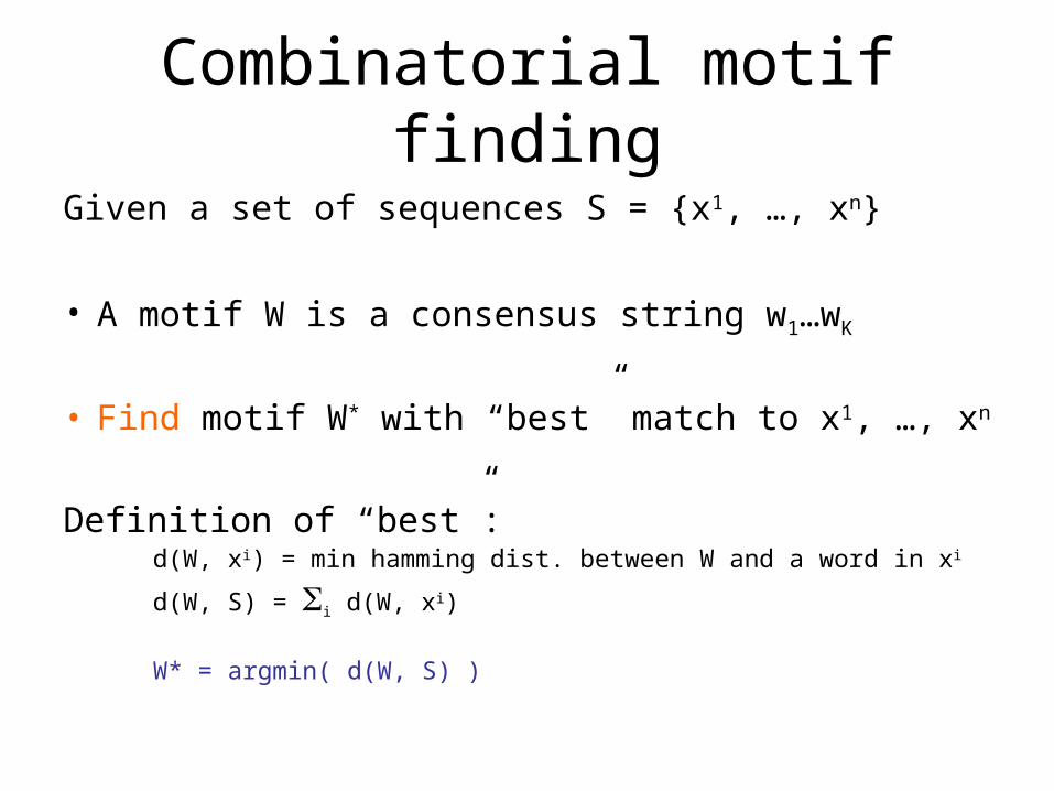
Combinatorial motif finding

Given a set of sequences S = {x1, …, xn}

• A motif W is a consensus string w1…wK

• Find motif W* with “best” match to x1, …, xn

Definition of “best”:d(W, xi) = min hamming dist. between W and a word in xi

d(W, S) = i d(W, xi)

W* = argmin( d(W, S) )

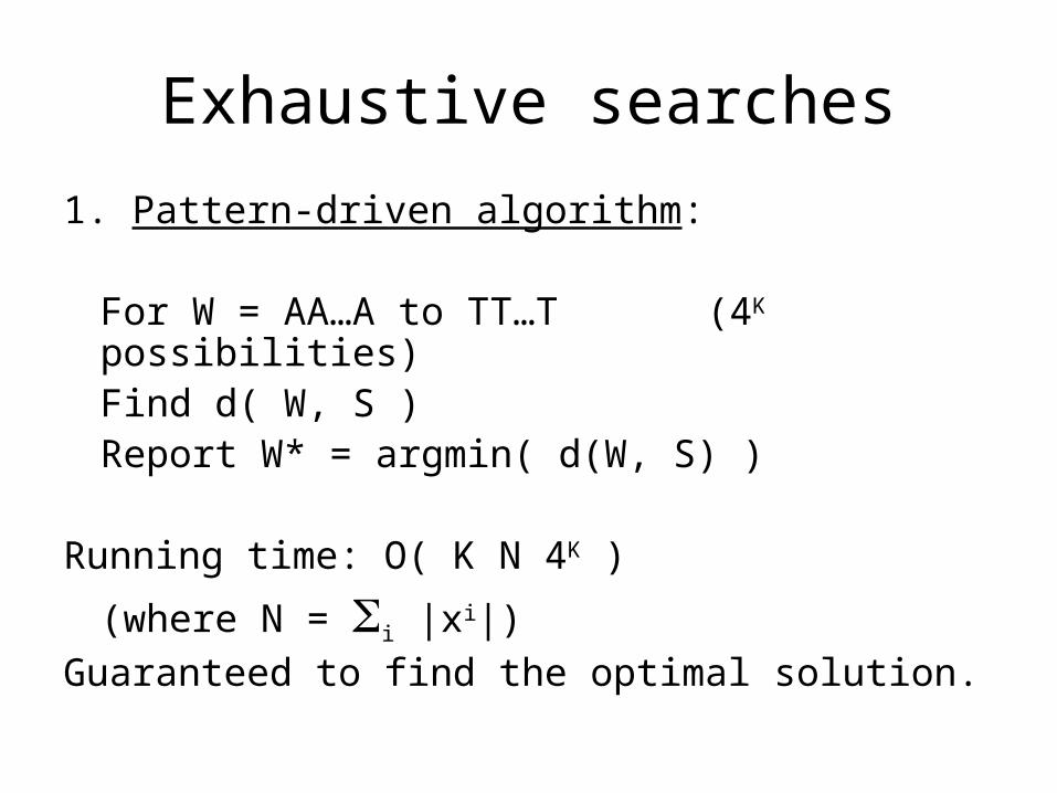
Exhaustive searches

1. Pattern-driven algorithm:

For W = AA…A to TT…T (4K possibilities)Find d( W, S )

Report W* = argmin( d(W, S) )

Running time: O( K N 4K )

(where N = i |xi|)

Guaranteed to find the optimal solution.

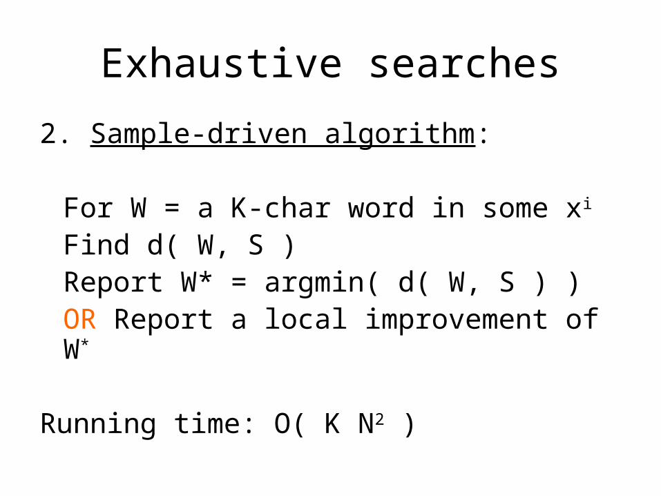
Exhaustive searches

2. Sample-driven algorithm:

For W = a K-char word in some xi

Find d( W, S )Report W* = argmin( d( W, S ) )OR Report a local improvement of W*

Running time: O( K N2 )

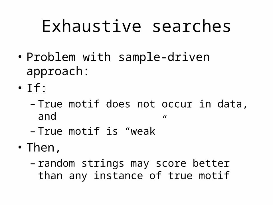
Exhaustive searches

• Problem with sample-driven approach:

• If:– True motif does not occur in data, and– True motif is “weak”

• Then,– random strings may score better than any

instance of true motif

Example

• E. coli. Promoter• “TATA-Box” ~ 10bp upstream of transcription

start• TACGAT• TAAAAT• TATACT• GATAAT• TATGAT• TATGTT

Consensus: TATAAT

Each instance differs at most 2 bases from the consensus

None of the instances matches the consensus perfectly

Heuristic methods

• Cannot afford exhaustive search on all patterns

• Sample-driven approaches may miss real patterns

• However, a real pattern should not differ too much from its instances in S

• Start from the space of all words in S, extend to the space with real patterns

Some of the popular tools

• Consensus (Hertz & Stormo, 1999)

• WINNOWER (Pevzner & Sze, 2000)

• MULTIPROFILER (Keich & Pevzner, 2002)

• PROJECTION (Buhler & Tompa, 2001)

• WEEDER (Pavesi et. al. 2001)

• And dozens of others

Consensus

Algorithm:

Cycle 1:For each word W in S

For each word W’ in SCreate alignment (gap free) of W, W’

Keep the C1 best alignments, A1, …, AC1

ACGGTTG , CGAACTT , GGGCTCT …ACGCCTG , AGAACTA , GGGGTGT …

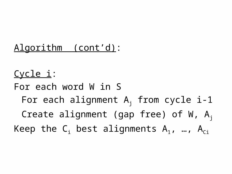
Algorithm (cont’d):

Cycle i:

For each word W in S

For each alignment Aj from cycle i-1

Create alignment (gap free) of W, Aj

Keep the Ci best alignments A1, …, ACi

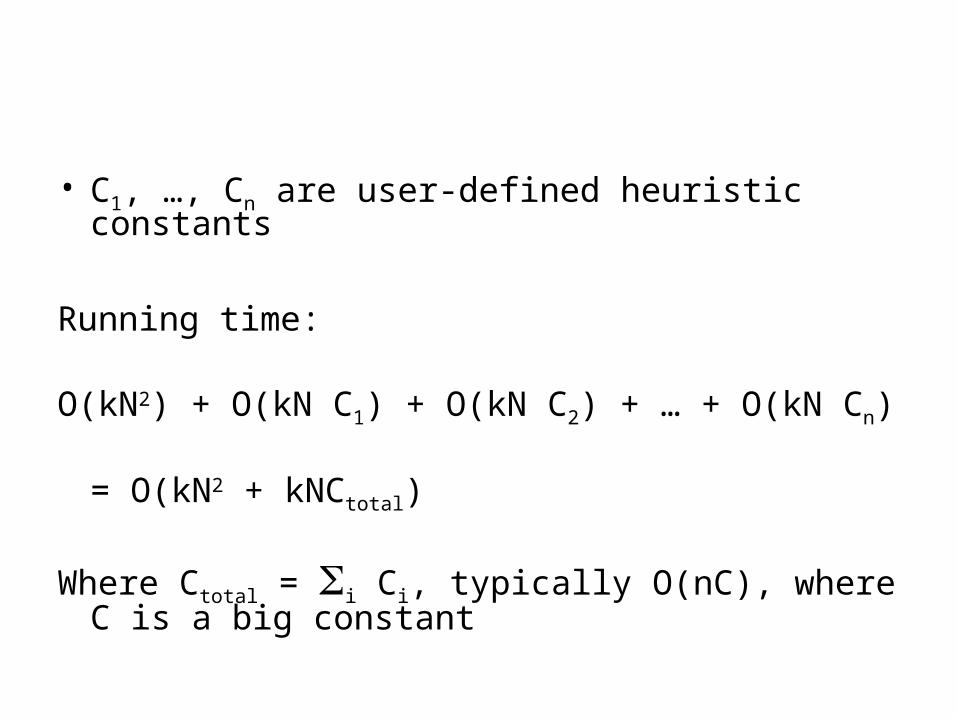
• C1, …, Cn are user-defined heuristic constants

Running time:

O(kN2) + O(kN C1) + O(kN C2) + … + O(kN Cn)

= O(kN2 + kNCtotal)

Where Ctotal = i Ci, typically O(nC), where C is a big constant

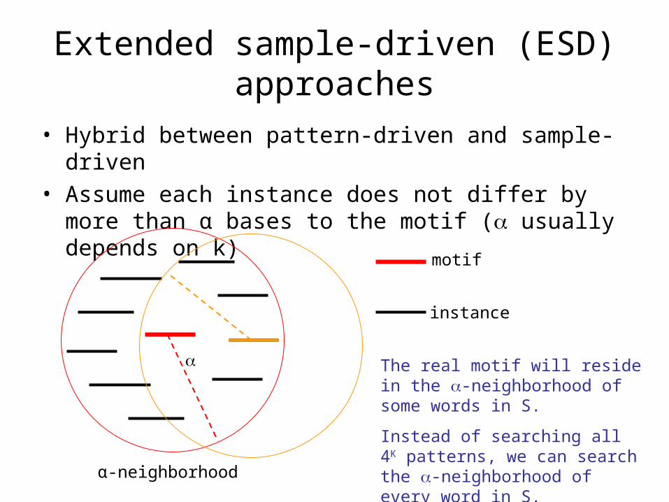
Extended sample-driven (ESD) approaches

• Hybrid between pattern-driven and sample-driven• Assume each instance does not differ by more than α

bases to the motif ( usually depends on k)

motif

instance

The real motif will reside in the -neighborhood of some words in S.

Instead of searching all 4K patterns, we can search the -neighborhood of every word in S.

α-neighborhood

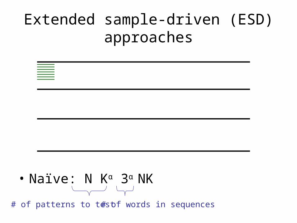
Extended sample-driven (ESD) approaches

• Naïve: N Kα 3α NK

# of patterns to test # of words in sequences

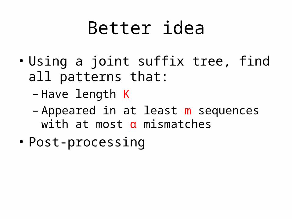
Better idea

• Using a joint suffix tree, find all patterns that:– Have length K– Appeared in at least m sequences with at

most α mismatches

• Post-processing

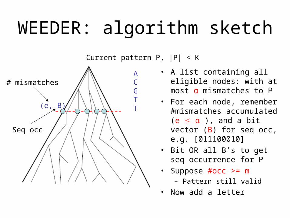
WEEDER: algorithm sketch

• A list containing all eligible nodes: with at most α mismatches to P

• For each node, remember #mismatches accumulated (e α ), and a bit vector (B) for seq occ, e.g. [011100010]

• Bit OR all B’s to get seq occurrence for P

• Suppose #occ >= m– Pattern still valid

• Now add a letter

ACGTT

Current pattern P, |P| < K

(e, B)

# mismatches

Seq occ

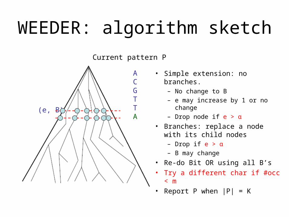
WEEDER: algorithm sketch

• Simple extension: no branches. – No change to B

– e may increase by 1 or no change

– Drop node if e > α

• Branches: replace a node with its child nodes– Drop if e > α

– B may change

• Re-do Bit OR using all B’s• Try a different char if #occ < m• Report P when |P| = K

ACGTTA

Current pattern P

(e, B)

WEEDER: complexity

• Can get all patterns in time O(Nn(K choose α) 3α) ~ O(N nKα 3α).

n: # sequences. Needed for Bit OR.

• Better than O(KN 4K) and O(N Kα 3α NK) since usually α << K

• Kα 3α may still be expensive for large K– E.g. K = 20, α = 6

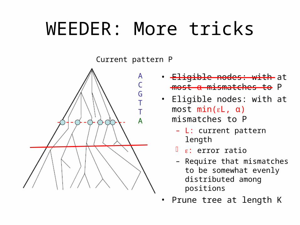
WEEDER: More tricks

• Eligible nodes: with at most α mismatches to P

• Eligible nodes: with at most min(L, α) mismatches to P– L: current pattern length : error ratio

– Require that mismatches to be somewhat evenly distributed among positions

• Prune tree at length K

ACGTTA

Current pattern P

Probabilistic modeling approaches

for motif finding

Probabilistic modeling approaches

• A motif model– Usually a PWM– M = (Pij), i = 1..4, j = 1..k, k: motif length

• A background model– Usually the distribution of base frequencies in

the genome (or other selected subsets of sequences)

– B = (bi), i = 1..4

• A word can be generated by M or B

Expectation-Maximization

• For any word W, P(W | M) = PW[1] 1 PW[2] 2…PW[K] K

P(W | B) = bW[1] bW[2] …bW[K]

• Let = P(M), i.e., the probability for any word to be generated by M.

• Then P(B) = 1 - • Can compute the posterior probability P(M|W)

and P(B|W) P(M|W) ~ P(W|M) * P(B|W) ~ P(W|B) * (1-)

Expectation-Maximization

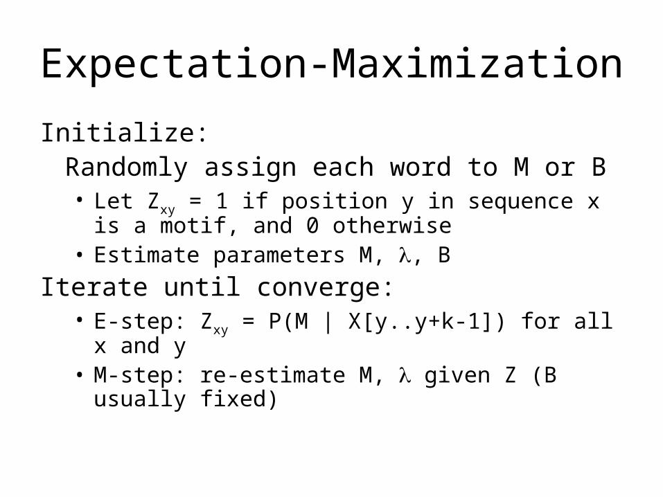
Initialize: Randomly assign each word to M or B• Let Zxy = 1 if position y in sequence x is a motif, and 0

otherwise• Estimate parameters M, , B

Iterate until converge:• E-step: Zxy = P(M | X[y..y+k-1]) for all x and y• M-step: re-estimate M, given Z (B usually fixed)

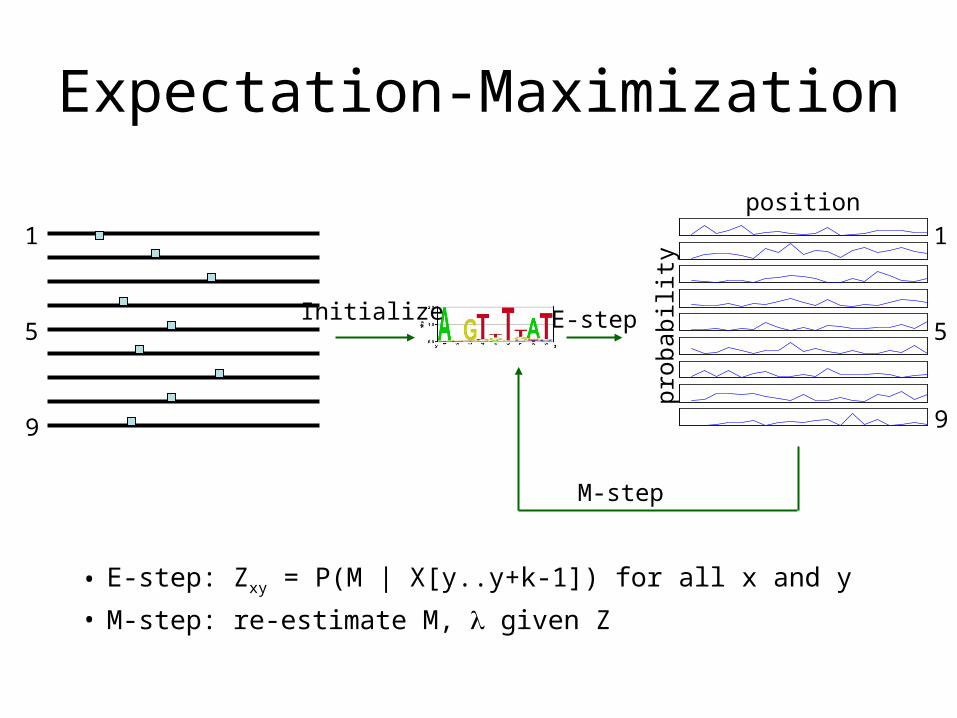
Expectation-Maximization

• E-step: Zxy = P(M | X[y..y+k-1]) for all x and y

• M-step: re-estimate M, given Z

Initialize E-step

M-step

prob

abili

ty

position

1

9

5

1

9

5

MEME

• Multiple EM for Motif Elicitation

• Bailey and Elkan, UCSD

• http://meme.sdsc.edu/

• Multiple starting points

• Multiple modes: ZOOPS, OOPS, TCM

Gibbs Sampling

• Another very useful technique for estimating missing parameters

• EM is deterministic– Often trapped by local optima

• Gibbs sampling: stochastic behavior to avoid local optima

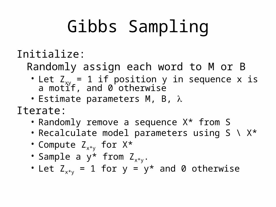
Gibbs Sampling

Initialize: Randomly assign each word to M or B• Let Zxy = 1 if position y in sequence x is a motif, and 0

otherwise• Estimate parameters M, B,

Iterate:• Randomly remove a sequence X* from S• Recalculate model parameters using S \ X*• Compute Zx*y for X*• Sample a y* from Zx*y. • Let Zx*y = 1 for y = y* and 0 otherwise

Gibbs Sampling

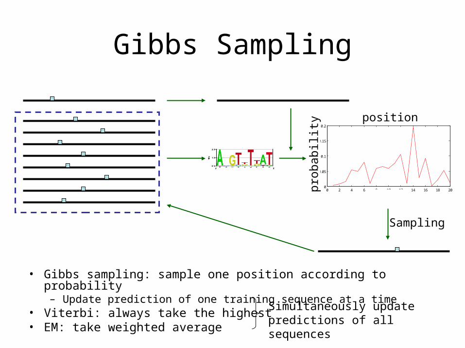
• Gibbs sampling: sample one position according to probability– Update prediction of one training sequence at a time

• Viterbi: always take the highest• EM: take weighted average

0 2 4 6 8 10 12 14 16 18 200

0.05

0.1

0.15

0.2

position

prob

abili

ty

Sampling

Simultaneously update predictions of all sequences

position

prob

abili

ty

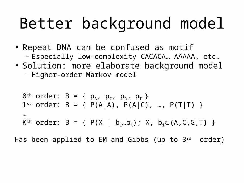
Better background model

• Repeat DNA can be confused as motif– Especially low-complexity CACACA… AAAAA, etc.

• Solution: more elaborate background model– Higher-order Markov model

0th order: B = { pA, pC, pG, pT }1st order: B = { P(A|A), P(A|C), …, P(T|T) }…Kth order: B = { P(X | b1…bK); X, bi{A,C,G,T} }

Has been applied to EM and Gibbs (up to 3rd order)

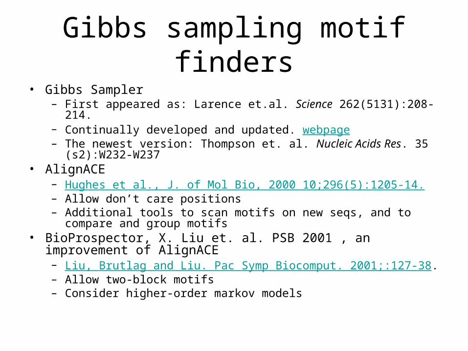
Gibbs sampling motif finders• Gibbs Sampler

– First appeared as: Larence et.al. Science 262(5131):208-214. – Continually developed and updated. webpage– The newest version: Thompson et. al. Nucleic Acids Res. 35 (s2):W232-

W237 • AlignACE

– Hughes et al., J. of Mol Bio, 2000 10;296(5):1205-14. – Allow don’t care positions– Additional tools to scan motifs on new seqs, and to compare and group

motifs• BioProspector, X. Liu et. al. PSB 2001 , an improvement of

AlignACE– Liu, Brutlag and Liu. Pac Symp Biocomput. 2001;:127-38. – Allow two-block motifs– Consider higher-order markov models

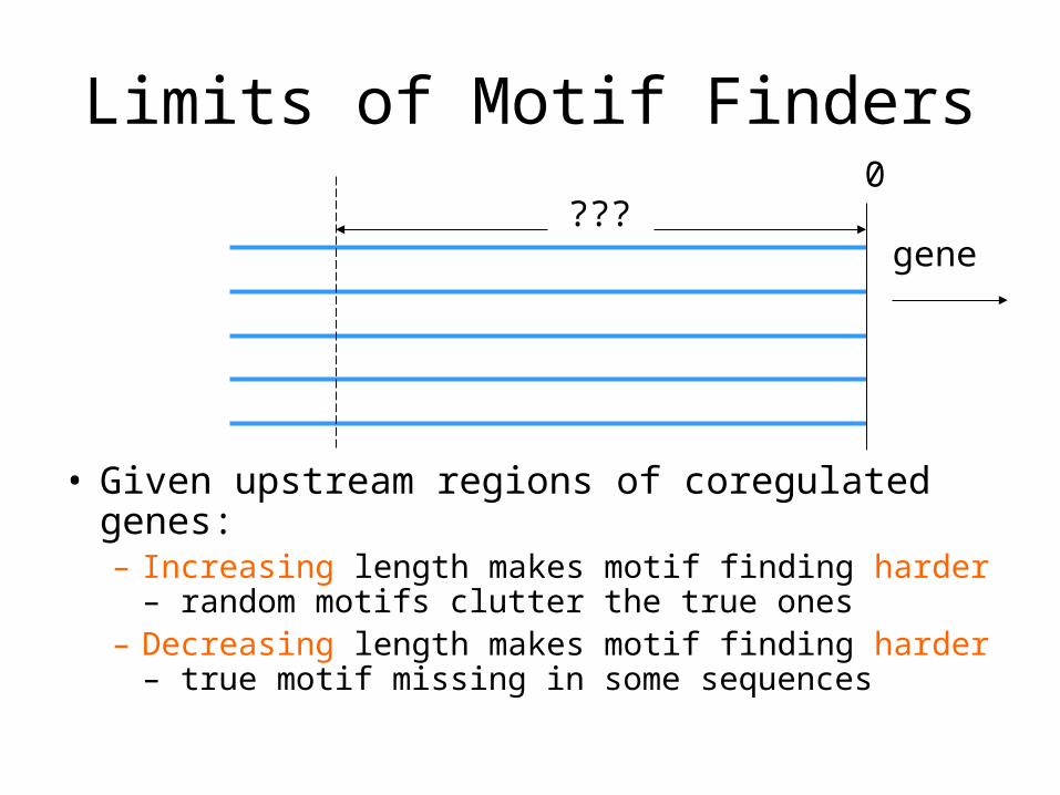
Limits of Motif Finders

• Given upstream regions of coregulated genes:– Increasing length makes motif finding harder –

random motifs clutter the true ones– Decreasing length makes motif finding harder – true

motif missing in some sequences

0

gene???

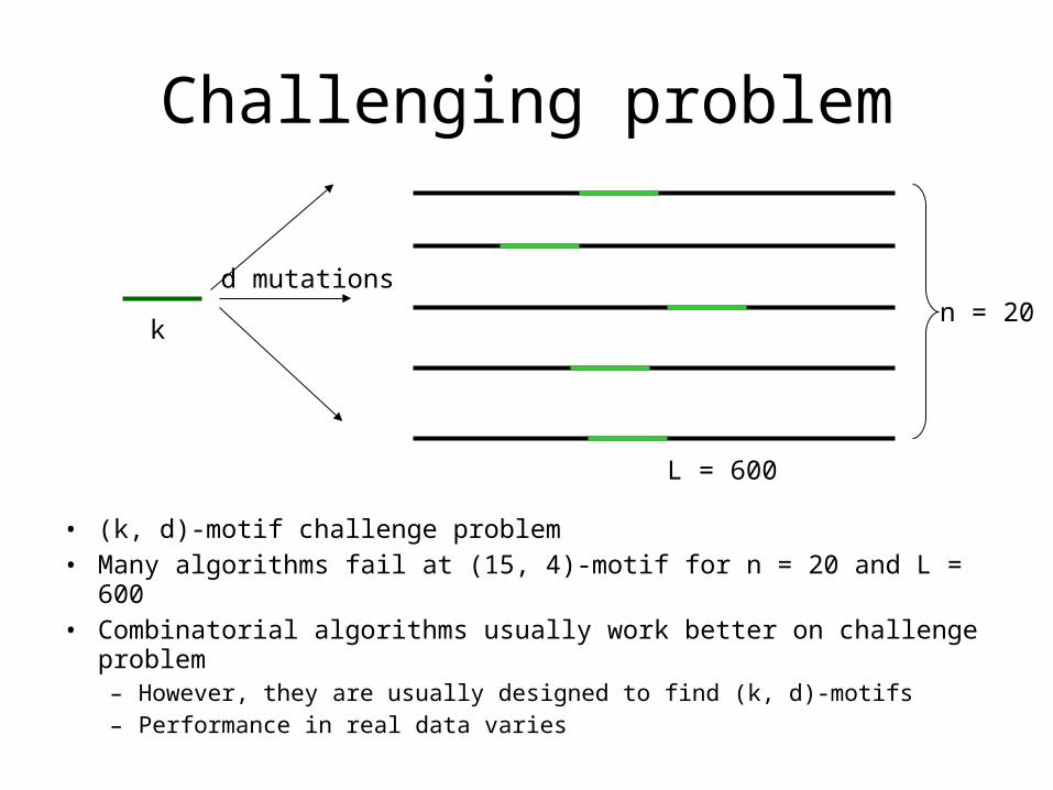
Challenging problem

• (k, d)-motif challenge problem• Many algorithms fail at (15, 4)-motif for n = 20 and L = 600• Combinatorial algorithms usually work better on challenge problem

– However, they are usually designed to find (k, d)-motifs– Performance in real data varies

k

d mutationsn = 20

L = 600

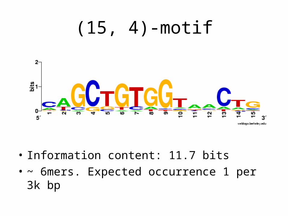
(15, 4)-motif

• Information content: 11.7 bits

• ~ 6mers. Expected occurrence 1 per 3k bp

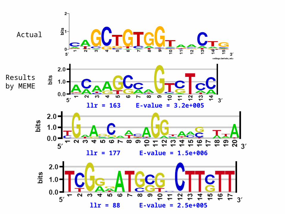
Actual

Results by MEME

llr = 163 E-value = 3.2e+005

llr = 177     E-value = 1.5e+006

llr = 88     E-value = 2.5e+005

Motif finding in practice

• Where the input come from?

• Possibility 1: microarray studies (later)

• Possibility 2: phylogenetic analysis (not covered)

• Possibility 3: ChIP-chip

• Possibility 4: ChIP-seq

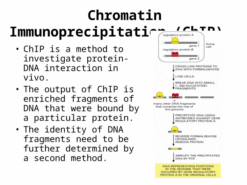
Chromatin Immunoprecipitation (ChIP)

• ChIP is a method to investigate protein-DNA interaction in vivo.

• The output of ChIP is enriched fragments of DNA that were bound by a particular protein.

• The identity of DNA fragments need to be further determined by a second method.

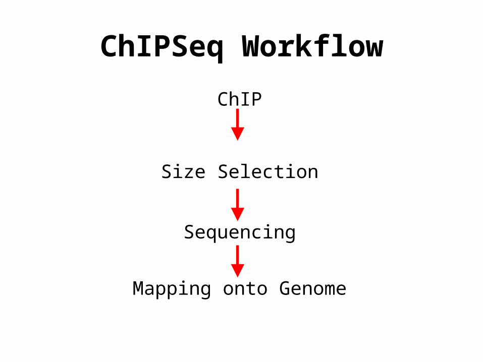
ChIPSeq Workflow

ChIP

Size Selection

Sequencing

Mapping onto Genome

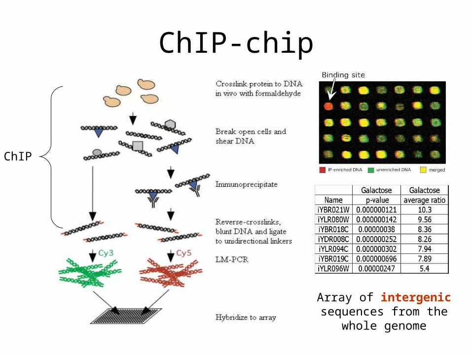
ChIP-chip

Array of intergenic sequences from the whole

genome

ChIP

How to make sense of the motifs?

• Each program usually reports a number of motifs (tens to hundreds)– Many motifs are variations of each other– Each program also report some different ones

• Each program has its own way of scoring motifs– Best scored motifs often not interesting– AAAAAAAA– ACACACAC– TATATATAT

How to make sense of the motifs?

• Now we’ve found some pretty-looking motifs– This is probably the easiest step

• What to do next?– Are they real?– How do we find more instances in the rest of

the genome?– What are their functional meaning?

• Motifs => regulatory networks

How to make sense of the motifs?

• Combine results from different algorithms usually helpful– Ones that appeared multiple times are probably more

interesting• Except simple repeats like AAAAA or ATATATATA

– Cluster motifs into groups.

• Compare with known motifs in database– TRANSFAC– JASPAR– YPD (yeast promoter database)

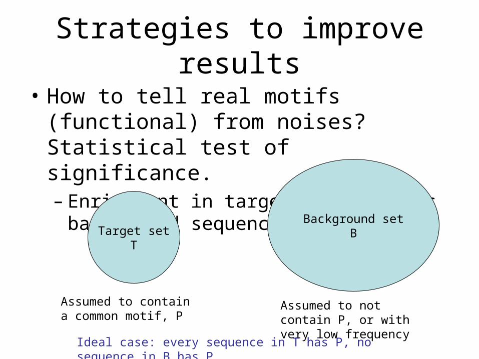
Strategies to improve results

• How to tell real motifs (functional) from noises? Statistical test of significance.– Enrichment in target sequences vs

background sequences

Target setT

Background setB

Assumed to contain a common motif, P

Assumed to not contain P, or with very low frequency

Ideal case: every sequence in T has P, no sequence in B has P

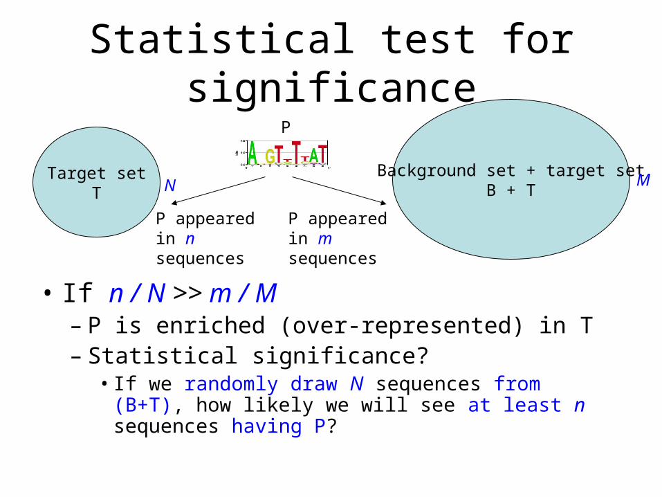
Statistical test for significance

• If n / N >> m / M– P is enriched (over-represented) in T– Statistical significance?

• If we randomly draw N sequences from (B+T), how likely we will see at least n sequences having P?

Target setT

Background set + target setB + TN M

P

P appeared in n sequences

P appeared in m sequences

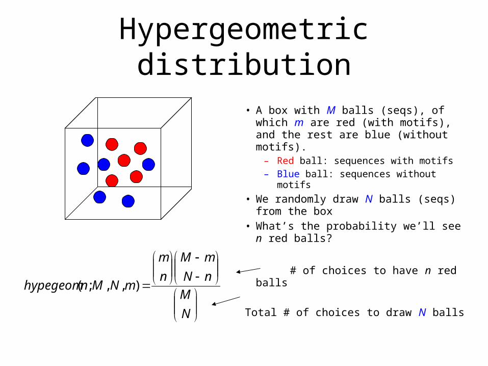
Hypergeometric distribution

• A box with M balls (seqs), of which m are red (with motifs), and the rest are blue (without motifs).

– Red ball: sequences with motifs– Blue ball: sequences without motifs

• We randomly draw N balls (seqs) from the box

• What’s the probability we’ll see n red balls?

# of choices to have n red balls

Total # of choices to draw N balls

N

M

nN

mM

n

m

mNMnhypegeom ),,;(

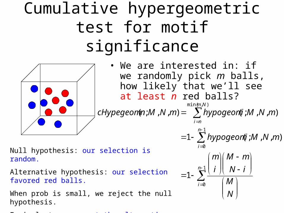
Cumulative hypergeometric test for motif significance

• We are interested in: if we randomly pick m balls, how likely that we’ll see at least n red balls?

1

0

1

0

),min(

1

),,;(1

),,;(),,;(

n

i

n

i

Nm

ni

N

M

iN

mM

i

m

mNMihypogeom

mNMihypogeommNMncHypegeom

Null hypothesis: our selection is random.

Alternative hypothesis: our selection favored red balls.

When prob is small, we reject the null hypothesis.

Equivalent: we accept the alternative hypothesis

(The number of red balls is larger than expected).

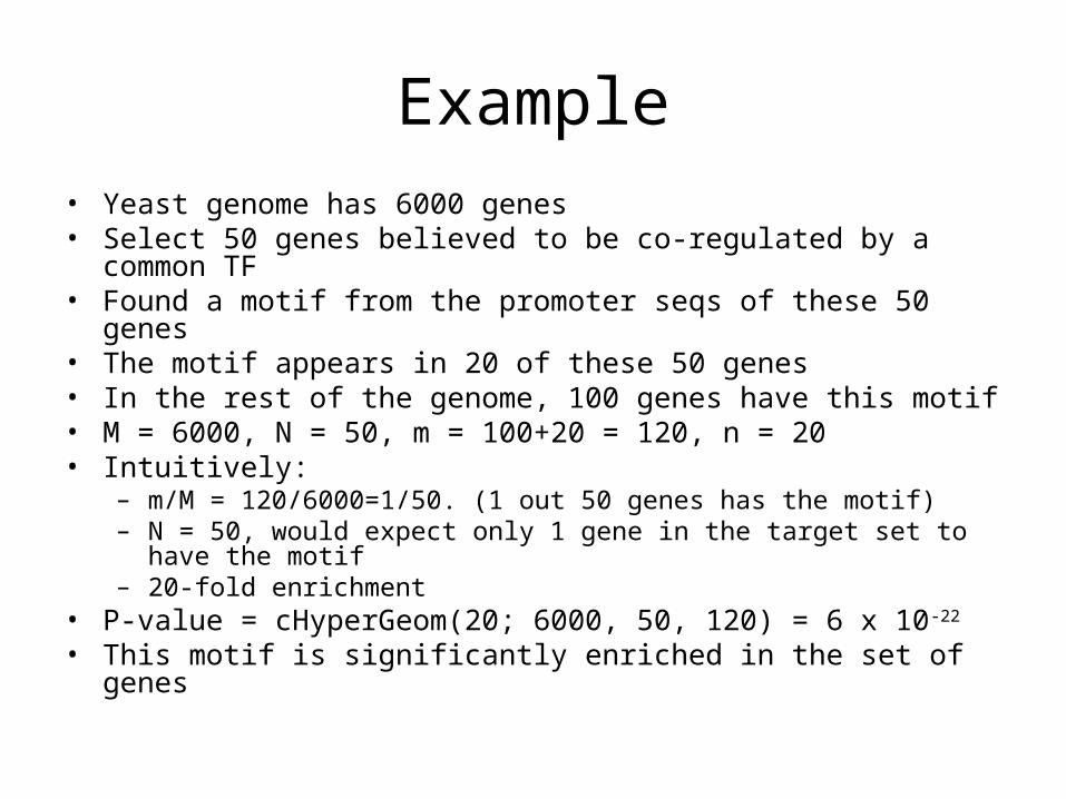
Example• Yeast genome has 6000 genes• Select 50 genes believed to be co-regulated by a common TF• Found a motif from the promoter seqs of these 50 genes• The motif appears in 20 of these 50 genes• In the rest of the genome, 100 genes have this motif• M = 6000, N = 50, m = 100+20 = 120, n = 20• Intuitively:

– m/M = 120/6000=1/50. (1 out 50 genes has the motif)– N = 50, would expect only 1 gene in the target set to have the motif – 20-fold enrichment

• P-value = cHyperGeom(20; 6000, 50, 120) = 6 x 10-22

• This motif is significantly enriched in the set of genes

ROC curve for motif significance

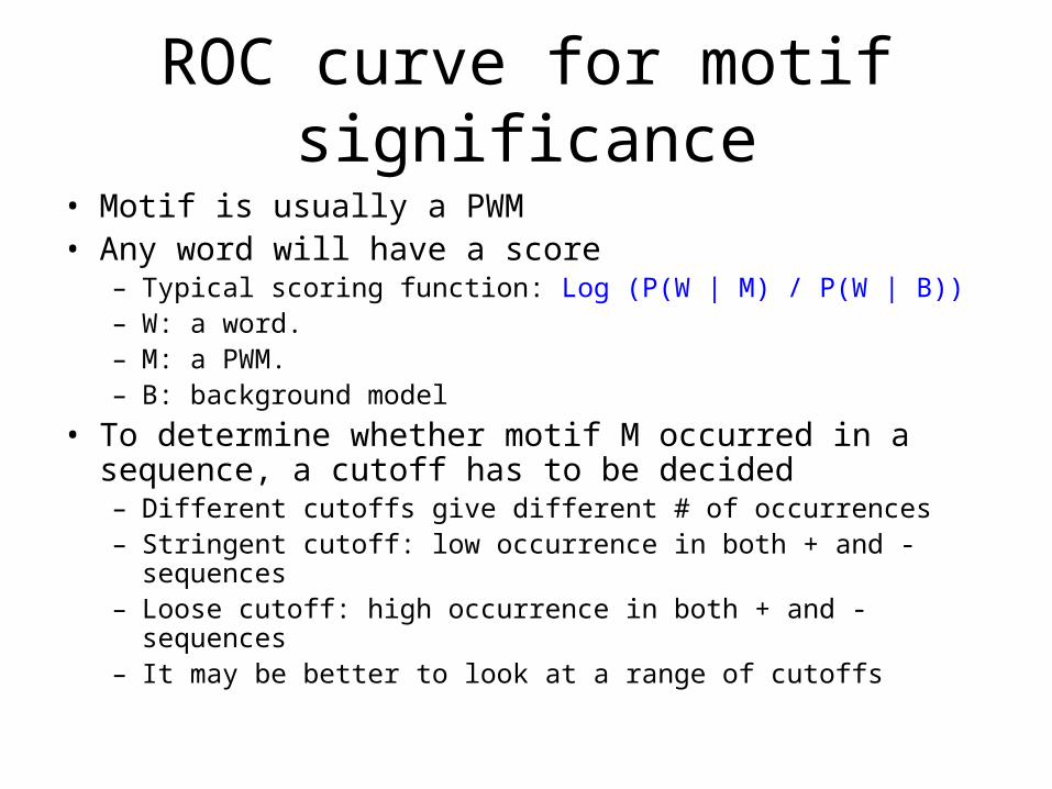
• Motif is usually a PWM• Any word will have a score

– Typical scoring function: Log (P(W | M) / P(W | B))– W: a word. – M: a PWM. – B: background model

• To determine whether motif M occurred in a sequence, a cutoff has to be decided– Different cutoffs give different # of occurrences– Stringent cutoff: low occurrence in both + and - sequences– Loose cutoff: high occurrence in both + and - sequences– It may be better to look at a range of cutoffs

ROC curve for motif significance

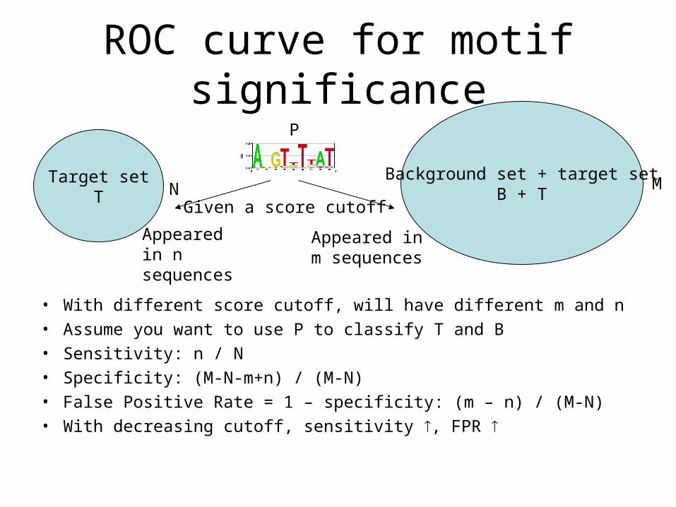
• With different score cutoff, will have different m and n• Assume you want to use P to classify T and B• Sensitivity: n / N• Specificity: (M-N-m+n) / (M-N)• False Positive Rate = 1 – specificity: (m – n) / (M-N)• With decreasing cutoff, sensitivity , FPR

Target setT

Background set + target setB + TN M

P

Appeared in n sequences

Appeared in m sequences

Given a score cutoff

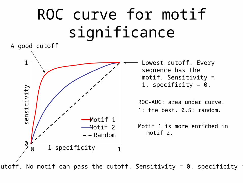
ROC curve for motif significance

ROC-AUC: area under curve.

1: the best. 0.5: random.

Motif 1 is more enriched in motif 2.

1-specificity

sens

itivi

ty

Motif 1Motif 2Random

A good cutoff

Highest cutoff. No motif can pass the cutoff. Sensitivity = 0. specificity = 1.

Lowest cutoff. Every sequence has the motif. Sensitivity = 1. specificity = 0.

0

1

10

Other strategies

• Cross-validation– Randomly divide sequences into 10 sets, hold 1 set

for test. – Do motif finding on 9 sets. Does the motif also appear

in the testing set?

• Phylogenetic conservation information– Does a motif also appears in the homologous genes

of another species?– Strongest evidence– However, will not be able to find species-specific ones

Other strategies

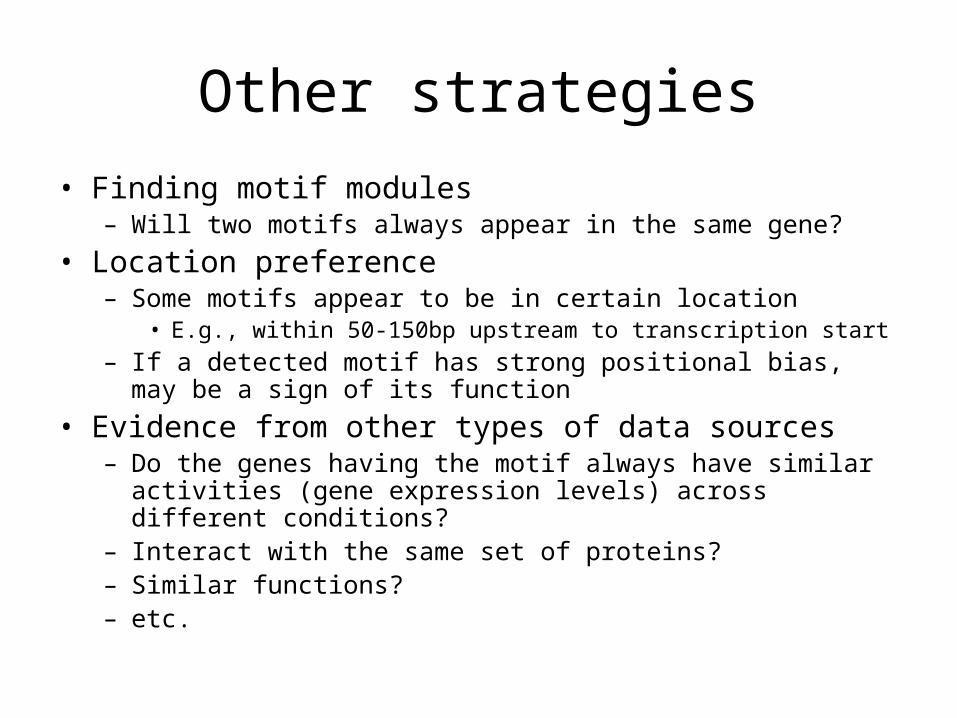
• Finding motif modules– Will two motifs always appear in the same gene?

• Location preference– Some motifs appear to be in certain location

• E.g., within 50-150bp upstream to transcription start

– If a detected motif has strong positional bias, may be a sign of its function

• Evidence from other types of data sources– Do the genes having the motif always have similar activities

(gene expression levels) across different conditions?– Interact with the same set of proteins?– Similar functions?– etc.

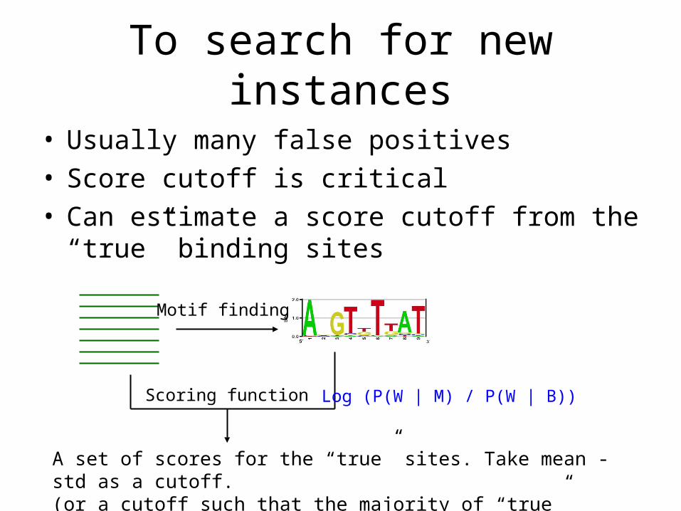
To search for new instances

• Usually many false positives• Score cutoff is critical• Can estimate a score cutoff from the “true”

binding sites

Motif finding

Scoring function

A set of scores for the “true” sites. Take mean - std as a cutoff. (or a cutoff such that the majority of “true” sites can be predicted).

Log (P(W | M) / P(W | B))

To search for new instances

• Use other information, such as positional biases of motifs to restrict the regions that a motif may appear

• Use gene expression data to help: the genes having the true motif should have similar activities– Risk of circular reasoning: most likely this is how you

get the initial sequences to do motif finding

• Phylogenetic conservation is the key

References

• D’haeseleer P (2006) What are DNA sequence motifs? NATURE BIOTECHNOLOGY, 24 (4):423-425

• D’haeseleer P (2006) How does DNA sequence motif discovery work? NATURE BIOTECHNOLOGY, 24 (8):959-961

• MacIsaac KD, Fraenkel E (2006) Practical strategies for discovering regulatory DNA sequence motifs. PLoS Comput Biol 2(4): e36

• Lawrence CE et. al. (1993) Detecting Subtle Sequence Signals: A Gibbs Sampling Strategy for Multiple Alignment, Science, 262(5131):208-214