CS 290H: Sparse Matrix Algorithms John R. Gilbert ([email protected])[email protected]...
119
CS 290H: Sparse Matrix Algorithms CS 290H: Sparse Matrix Algorithms John R. Gilbert ( [email protected] ) http://www.cs.ucsb.edu/~gilbert/cs29 0hFall2004
-
date post
20-Dec-2015 -
Category
Documents
-
view
338 -
download
2
Transcript of CS 290H: Sparse Matrix Algorithms John R. Gilbert ([email protected])[email protected]...
CS 290H: Sparse Matrix AlgorithmsCS 290H: Sparse Matrix Algorithms
John R. Gilbert ([email protected])
http://www.cs.ucsb.edu/~gilbert/cs290hFall2004
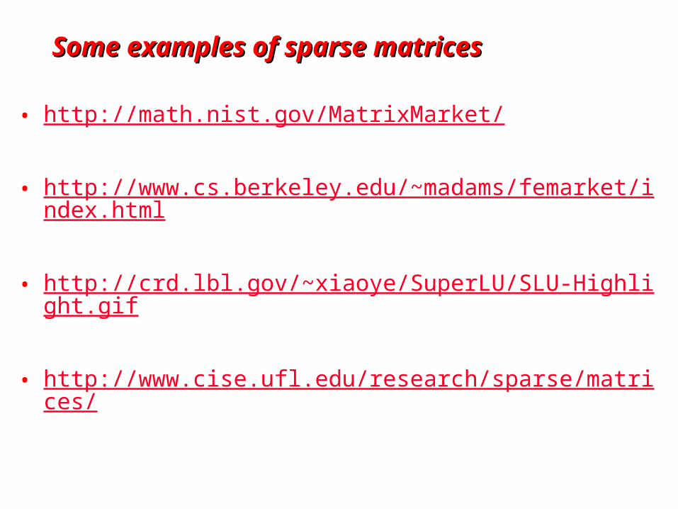
Some examples of sparse matricesSome examples of sparse matrices
• http://math.nist.gov/MatrixMarket/
• http://www.cs.berkeley.edu/~madams/femarket/index.html
• http://crd.lbl.gov/~xiaoye/SuperLU/SLU-Highlight.gif
• http://www.cise.ufl.edu/research/sparse/matrices/
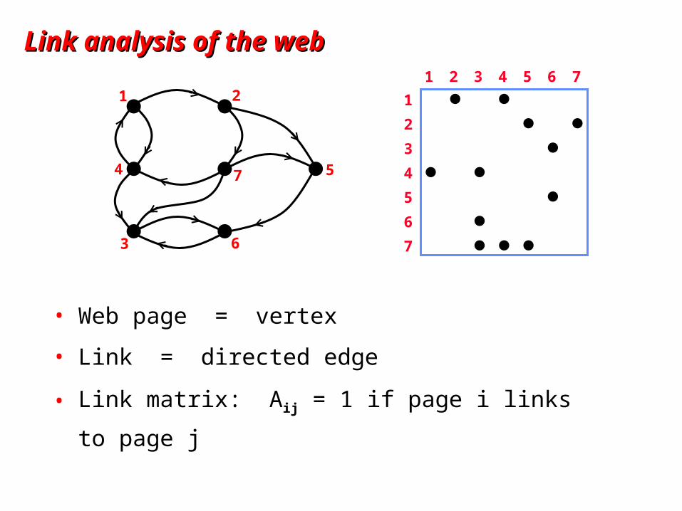
Link analysis of the webLink analysis of the web
• Web page = vertex
• Link = directed edge
• Link matrix: Aij = 1 if page i links to page j
1 2
3
4 7
6
5
1 52 3 4 6 7
1
5
2
3
4
6
7
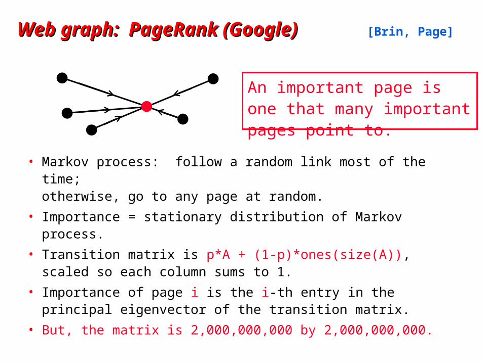
Web graph: PageRank (Google) Web graph: PageRank (Google) [Brin, Page]
• Markov process: follow a random link most of the time; otherwise, go to any page at random.
• Importance = stationary distribution of Markov process.
• Transition matrix is p*A + (1-p)*ones(size(A)), scaled so each column sums to 1.
• Importance of page i is the i-th entry in the principal eigenvector of the transition matrix.
• But, the matrix is 2,000,000,000 by 2,000,000,000.
An important page is one that many important pages point to.
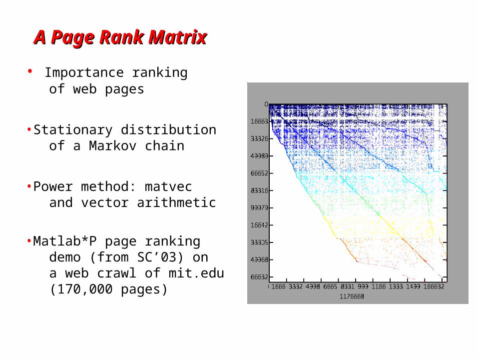
A Page Rank MatrixA Page Rank Matrix
• Importance ranking of web pages
•Stationary distribution of a Markov chain
•Power method: matvec and vector arithmetic
•Matlab*P page ranking demo (from SC’03) on a web crawl of mit.edu (170,000 pages)
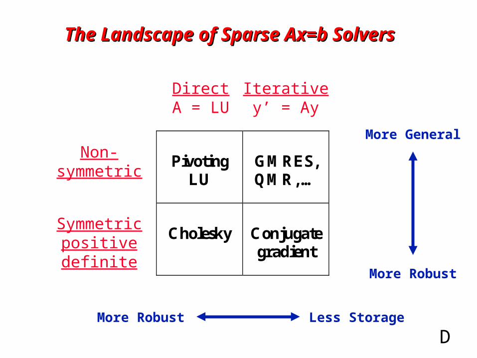
The Landscape of Sparse Ax=b SolversThe Landscape of Sparse Ax=b Solvers
Pivoting
LU
GMRES, QMR, …
Cholesky
Conjugate gradient
DirectA = LU
Iterativey’ = Ay
Non-symmetric
Symmetricpositivedefinite
More Robust Less Storage
More Robust
More General
D
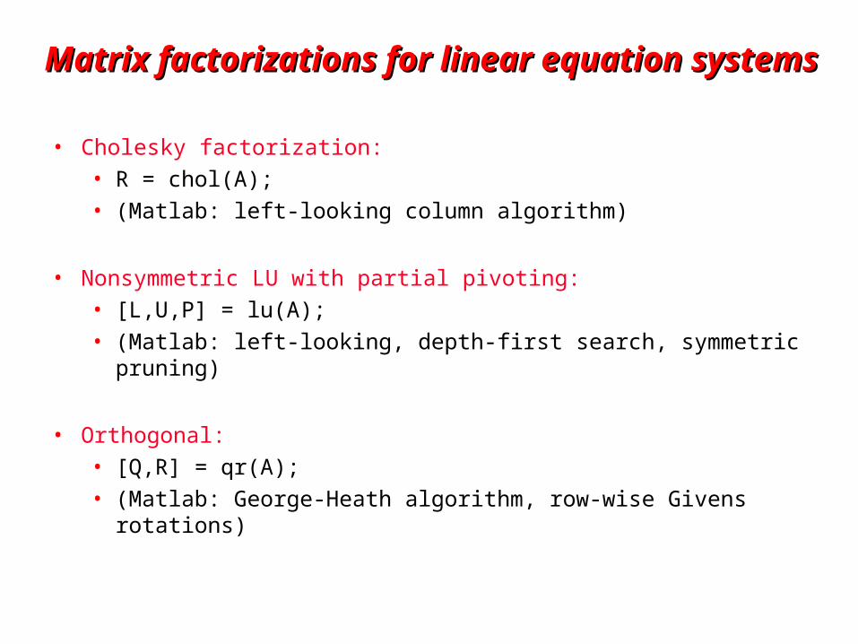
Matrix factorizations for linear equation systemsMatrix factorizations for linear equation systems
• Cholesky factorization:• R = chol(A);• (Matlab: left-looking column algorithm)
• Nonsymmetric LU with partial pivoting:• [L,U,P] = lu(A);• (Matlab: left-looking, depth-first search, symmetric pruning)
• Orthogonal: • [Q,R] = qr(A);• (Matlab: George-Heath algorithm, row-wise Givens rotations)
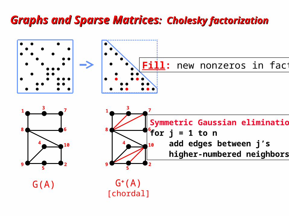
Graphs and Sparse MatricesGraphs and Sparse Matrices: Cholesky factorization: Cholesky factorization
10
13
2
4
5
6
7
8
9
10
13
2
4
5
6
7
8
9
G(A) G+(A)[chordal]
Symmetric Gaussian elimination:for j = 1 to n add edges between j’s higher-numbered neighbors
Fill: new nonzeros in factor
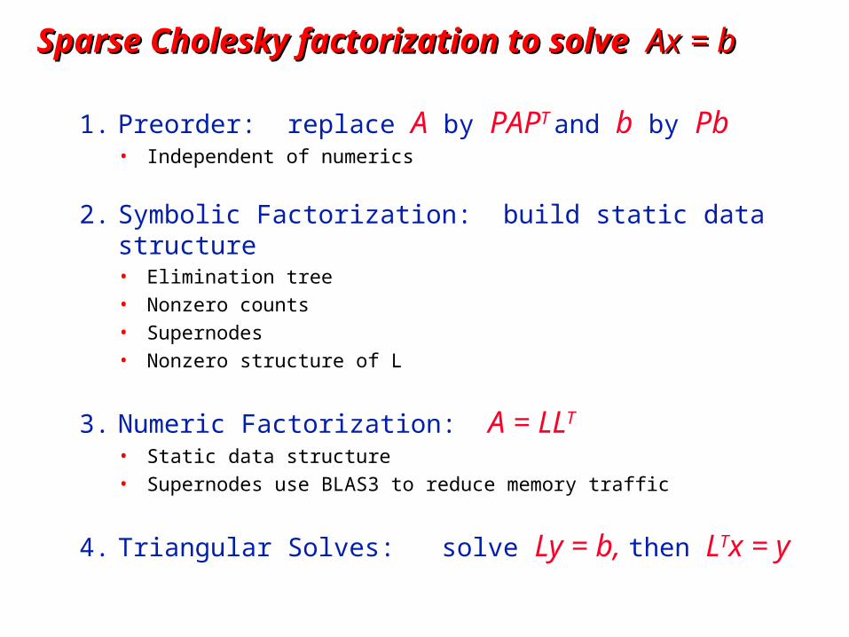
1. Preorder: replace A by PAPT and b by Pb• Independent of numerics
2. Symbolic Factorization: build static data structure• Elimination tree
• Nonzero counts
• Supernodes
• Nonzero structure of L
3. Numeric Factorization: A = LLT
• Static data structure
• Supernodes use BLAS3 to reduce memory traffic
4. Triangular Solves: solve Ly = b, then LTx = y
Sparse Cholesky factorization to solve Sparse Cholesky factorization to solve Ax = bAx = b
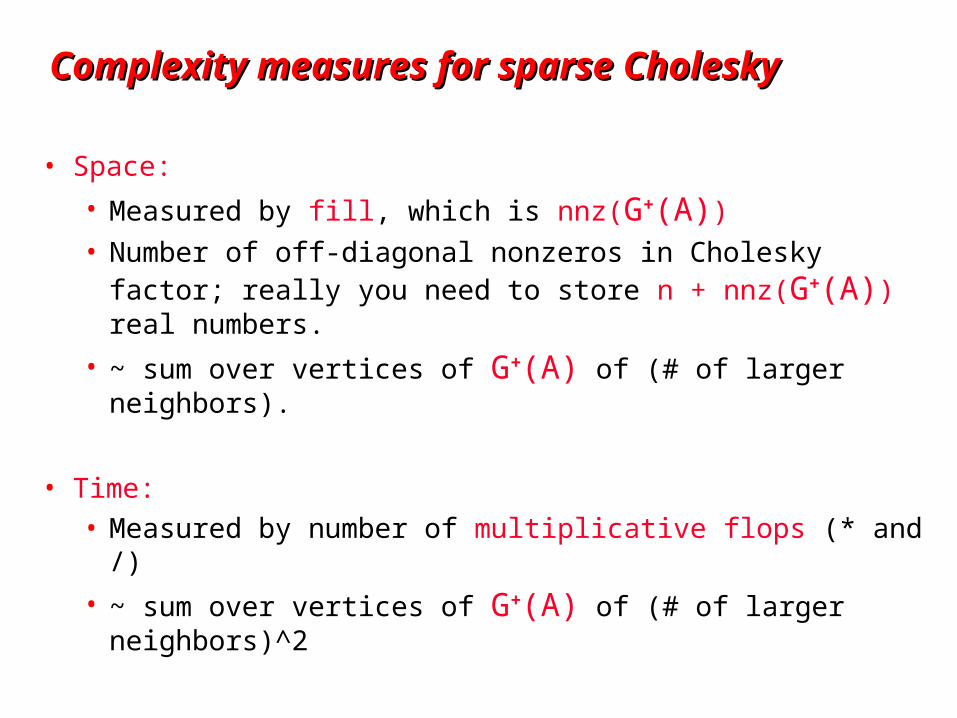
Complexity measures for sparse CholeskyComplexity measures for sparse Cholesky
• Space:
• Measured by fill, which is nnz(G+(A))• Number of off-diagonal nonzeros in Cholesky factor;
really you need to store n + nnz(G+(A)) real numbers.
• ~ sum over vertices of G+(A) of (# of larger neighbors).
• Time:• Measured by number of multiplicative flops (* and /)
• ~ sum over vertices of G+(A) of (# of larger neighbors)^2
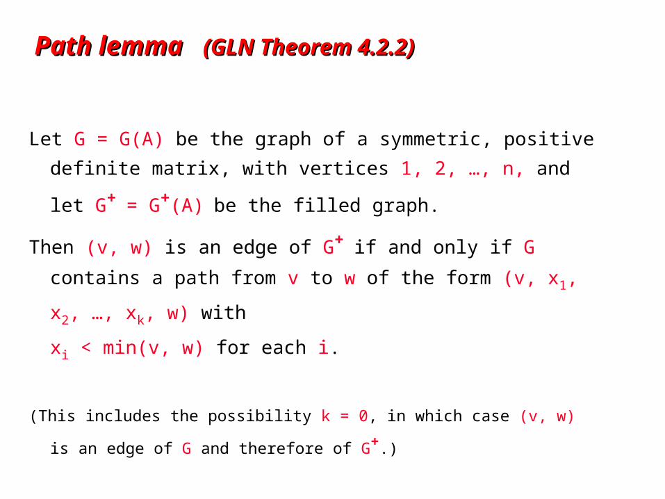
Path lemma Path lemma (GLN Theorem 4.2.2)(GLN Theorem 4.2.2)
Let G = G(A) be the graph of a symmetric, positive definite
matrix, with vertices 1, 2, …, n, and let G+ = G+(A) be the
filled graph.
Then (v, w) is an edge of G+ if and only if G contains a path
from v to w of the form (v, x1, x2, …, xk, w) with
xi < min(v, w) for each i.
(This includes the possibility k = 0, in which case (v, w) is an edge of G
and therefore of G+.)
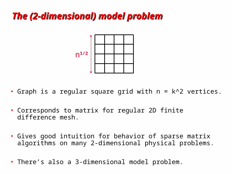
The (2-dimensional) model problemThe (2-dimensional) model problem
• Graph is a regular square grid with n = k^2 vertices.
• Corresponds to matrix for regular 2D finite difference mesh.
• Gives good intuition for behavior of sparse matrix algorithms on many 2-dimensional physical problems.
• There’s also a 3-dimensional model problem.
n1/2
Permutations of the 2-D model problemPermutations of the 2-D model problem
• Theorem: With the natural permutation, the n-vertex model problem has (n3/2) fill.
• Theorem: With any permutation, the n-vertex model problem has (n log n) fill.
• Theorem: With a nested dissection permutation, the n-vertex model problem has O(n log n) fill.
Nested dissection orderingNested dissection ordering
• A separator in a graph G is a set S of vertices whose removal leaves at least two connected components.
• A nested dissection ordering for an n-vertex graph G numbers its vertices from 1 to n as follows:
• Find a separator S, whose removal leaves connected components T1, T2, …, Tk
• Number the vertices of S from n-|S|+1 to n.• Recursively, number the vertices of each component:
T1 from 1 to |T1|, T2 from |T1|+1 to |T1|+|T2|, etc.
• If a component is small enough, number it arbitrarily.
• It all boils down to finding good separators!
Separators in theorySeparators in theory
• If G is a planar graph with n vertices, there exists a set of at most sqrt(6n) vertices whose removal leaves no connected component with more than 2n/3 vertices. (“Planar graphs have sqrt(n)-separators.”)
• “Well-shaped” finite element meshes in 3 dimensions have n2/3 - separators.
• Also some other classes of graphs – trees, graphs of bounded genus, chordal graphs, bounded-excluded-minor graphs, …
• Mostly these theorems come with efficient algorithms, but they aren’t used much.
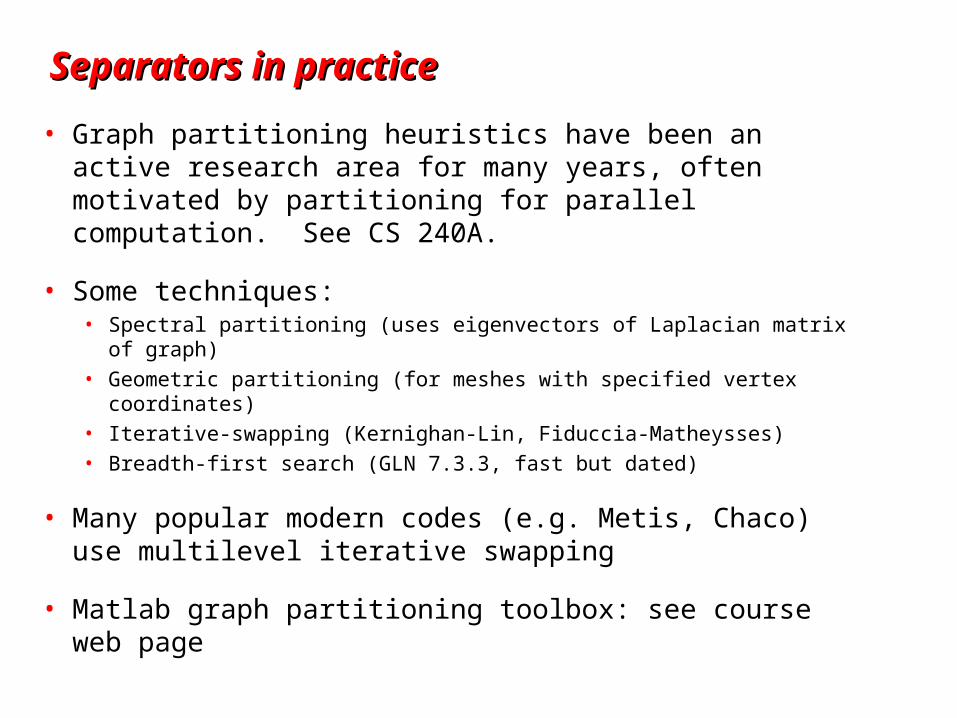
Separators in practiceSeparators in practice
• Graph partitioning heuristics have been an active research area for many years, often motivated by partitioning for parallel computation. See CS 240A.
• Some techniques:• Spectral partitioning (uses eigenvectors of Laplacian matrix of graph)
• Geometric partitioning (for meshes with specified vertex coordinates)
• Iterative-swapping (Kernighan-Lin, Fiduccia-Matheysses)
• Breadth-first search (GLN 7.3.3, fast but dated)
• Many popular modern codes (e.g. Metis, Chaco) use multilevel iterative swapping
• Matlab graph partitioning toolbox: see course web page
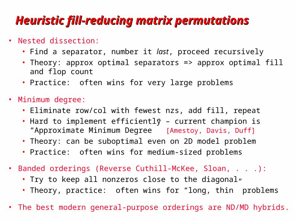
Heuristic fill-reducing matrix permutationsHeuristic fill-reducing matrix permutations
• Nested dissection: • Find a separator, number it last, proceed recursively• Theory: approx optimal separators => approx optimal fill and flop count• Practice: often wins for very large problems
• Minimum degree: • Eliminate row/col with fewest nzs, add fill, repeat• Hard to implement efficiently – current champion is
“Approximate Minimum Degree” [Amestoy, Davis, Duff]
• Theory: can be suboptimal even on 2D model problem• Practice: often wins for medium-sized problems
• Banded orderings (Reverse Cuthill-McKee, Sloan, . . .):• Try to keep all nonzeros close to the diagonal• Theory, practice: often wins for “long, thin” problems
• The best modern general-purpose orderings are ND/MD hybrids.
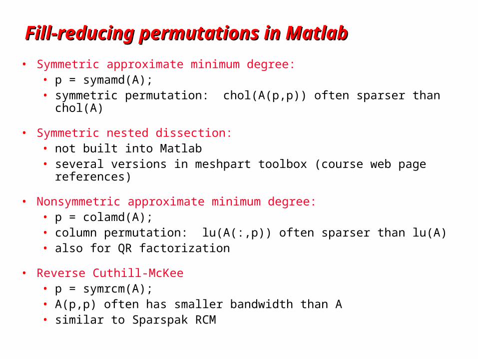
Fill-reducing permutations in MatlabFill-reducing permutations in Matlab
• Symmetric approximate minimum degree:• p = symamd(A); • symmetric permutation: chol(A(p,p)) often sparser than chol(A)
• Symmetric nested dissection:• not built into Matlab• several versions in meshpart toolbox (course web page references)
• Nonsymmetric approximate minimum degree:• p = colamd(A);• column permutation: lu(A(:,p)) often sparser than lu(A)• also for QR factorization
• Reverse Cuthill-McKee• p = symrcm(A);• A(p,p) often has smaller bandwidth than A• similar to Sparspak RCM
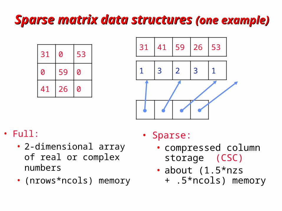
Sparse matrix data structures Sparse matrix data structures (one example)(one example)
• Full: • 2-dimensional array of
real or complex numbers• (nrows*ncols) memory
31 0 53
0 59 0
41 26 0
31 41 59 26 53
1 3 2 3 1
• Sparse: • compressed column
storage (CSC)• about (1.5*nzs + .5*ncols)
memory
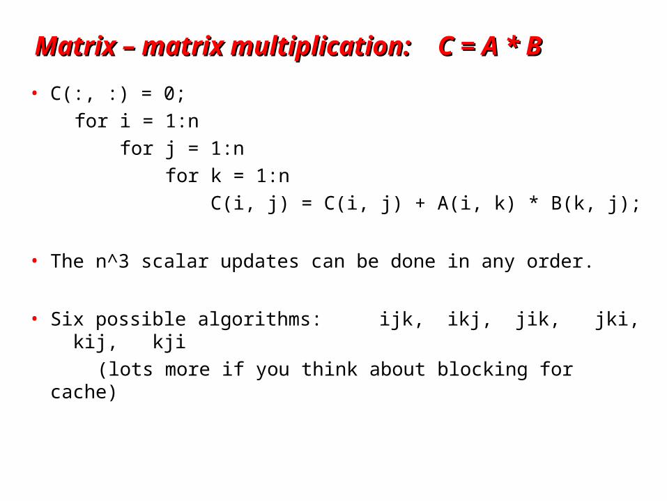
Matrix – matrix multiplication: C = A * BMatrix – matrix multiplication: C = A * B
• C(:, :) = 0;
for i = 1:n
for j = 1:n
for k = 1:n
C(i, j) = C(i, j) + A(i, k) * B(k, j);
• The n^3 scalar updates can be done in any order.
• Six possible algorithms: ijk, ikj, jik, jki, kij, kji
(lots more if you think about blocking for cache)
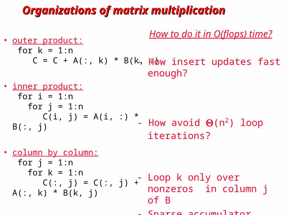
Organizations of matrix multiplicationOrganizations of matrix multiplication
• outer product: for k = 1:n C = C + A(:, k) * B(k, :)
• inner product: for i = 1:n for j = 1:n C(i, j) = A(i, :) * B(:, j)
• column by column: for j = 1:n for k = 1:n C(:, j) = C(:, j) + A(:, k) * B(k, j)
How to do it in O(flops) time?
- How insert updates fast enough?
- How avoid (n2) loop iterations?
- Loop k only over nonzeros in column j of B
- Sparse accumulator
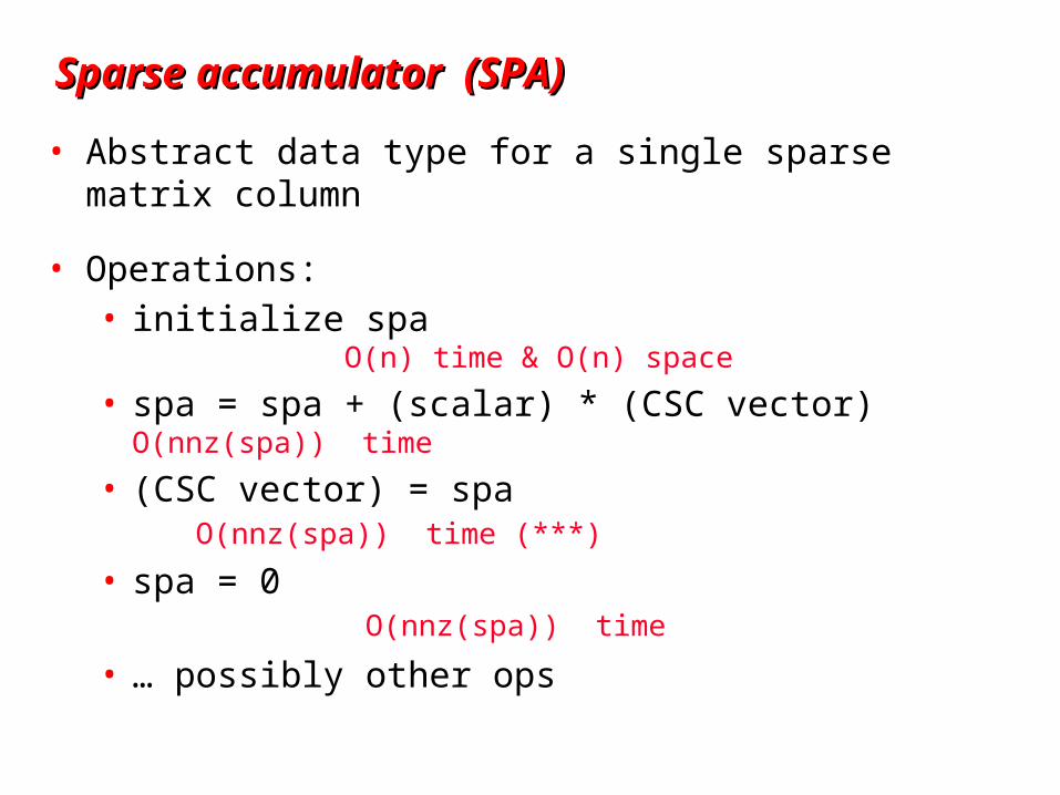
Sparse accumulator (SPA)Sparse accumulator (SPA)
• Abstract data type for a single sparse matrix column
• Operations:• initialize spa O(n) time & O(n) space
• spa = spa + (scalar) * (CSC vector) O(nnz(spa)) time
• (CSC vector) = spa O(nnz(spa)) time (***)
• spa = 0 O(nnz(spa)) time
• … possibly other ops
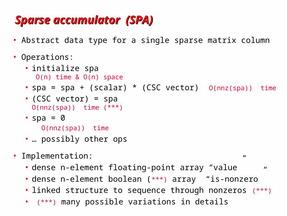
• Implementation:• dense n-element floating-point array “value”• dense n-element boolean (***) array “is-nonzero”• linked structure to sequence through nonzeros (***)• (***) many possible variations in details
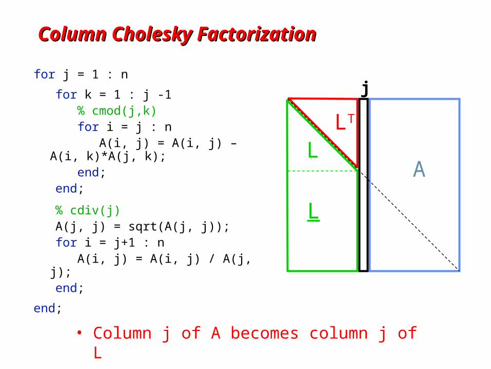
Column Cholesky FactorizationColumn Cholesky Factorization
for j = 1 : n
for k = 1 : j -1 % cmod(j,k) for i = j : n A(i, j) = A(i, j) – A(i, k)*A(j, k); end; end;
% cdiv(j) A(j, j) = sqrt(A(j, j)); for i = j+1 : n A(i, j) = A(i, j) / A(j, j); end;
end;
• Column j of A becomes column j of L
L
LLT
A
j
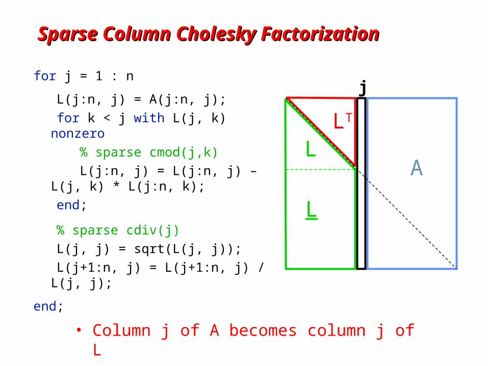
Sparse Column Cholesky FactorizationSparse Column Cholesky Factorization
for j = 1 : n
L(j:n, j) = A(j:n, j);
for k < j with L(j, k) nonzero
% sparse cmod(j,k)
L(j:n, j) = L(j:n, j) – L(j, k) * L(j:n, k);
end;
% sparse cdiv(j)
L(j, j) = sqrt(L(j, j));
L(j+1:n, j) = L(j+1:n, j) / L(j, j);
end;
• Column j of A becomes column j of L
L
LLT
A
j
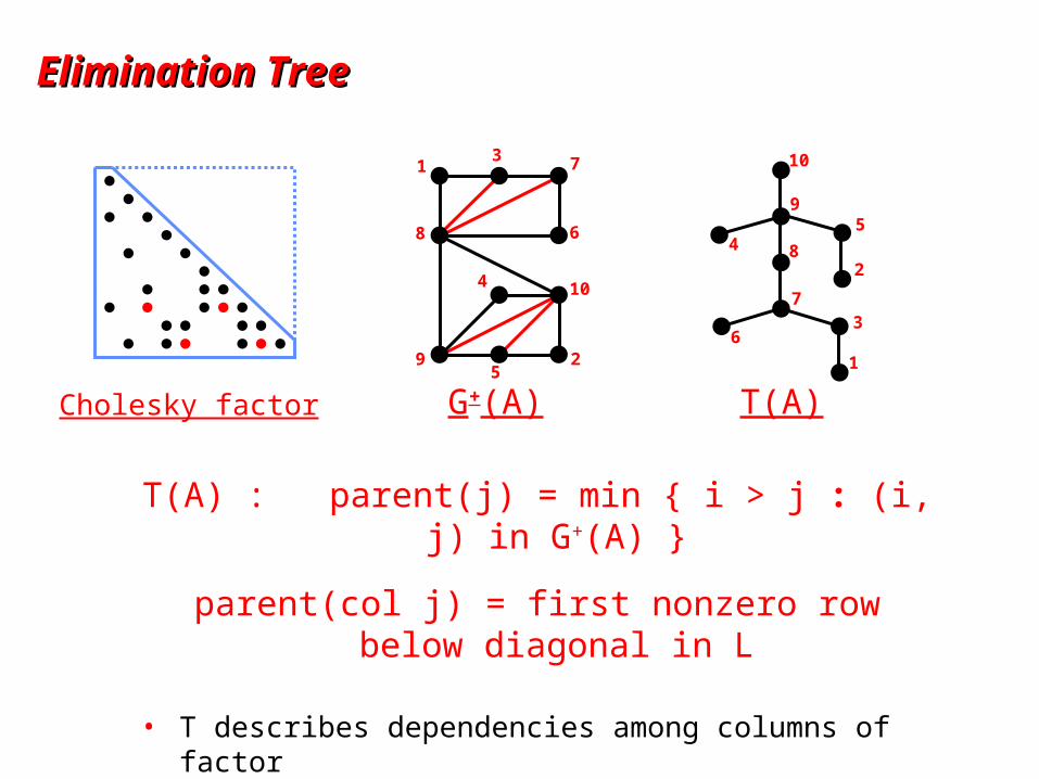
Elimination TreeElimination Tree
10
13
2
4
5
6
7
8
9
Cholesky factor G+(A) T(A)
10
1
3
2
45
6
7
8
9
T(A) : parent(j) = min { i > j : (i, j) in G+(A) }
parent(col j) = first nonzero row below diagonal in L
• T describes dependencies among columns of factor• Can compute G+(A) easily from T• Can compute T from G(A) in almost linear time
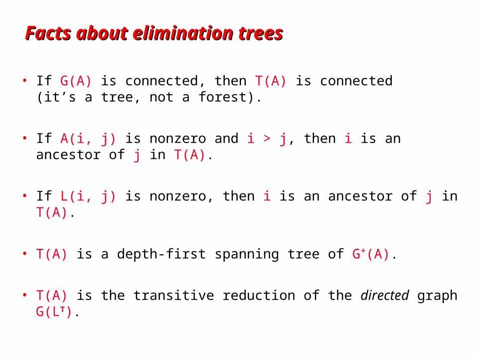
Facts about elimination treesFacts about elimination trees
• If G(A) is connected, then T(A) is connected (it’s a tree, not a forest).
• If A(i, j) is nonzero and i > j, then i is an ancestor of j in T(A).
• If L(i, j) is nonzero, then i is an ancestor of j in T(A).
• T(A) is a depth-first spanning tree of G+(A).
• T(A) is the transitive reduction of the directed graph G(LT).
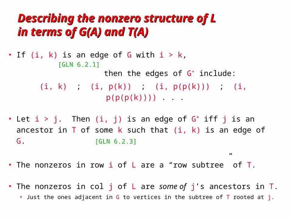
Describing the nonzero structure of L Describing the nonzero structure of L in terms of G(A) and T(A)in terms of G(A) and T(A)
• If (i, k) is an edge of G with i > k, [GLN 6.2.1] then the edges of G+ include:
(i, k) ; (i, p(k)) ; (i, p(p(k))) ; (i, p(p(p(k)))) . . .
• Let i > j. Then (i, j) is an edge of G+ iff j is an ancestor in T of
some k such that (i, k) is an edge of G. [GLN 6.2.3]
• The nonzeros in row i of L are a “row subtree” of T.
• The nonzeros in col j of L are some of j’s ancestors in T.• Just the ones adjacent in G to vertices in the subtree of T rooted at j.

Nested dissection fill boundsNested dissection fill bounds
• Theorem: With a nested dissection ordering using sqrt(n)-separators, any n-vertex planar graph has O(n log n) fill.• We’ll prove this assuming bounded vertex degree, but it’s true anyway.
• Corollary: With a nested dissection ordering, the n-vertex model problem has O(n log n) fill.
• Theorem: If a graph and all its subgraphs have O(na)-separators for some a >1/2, then it has an ordering with O(n2a) fill.• With a = 2/3, this applies to well-shaped 3-D finite element meshes
• In all these cases factorization time, or flop count, is O(n3a).
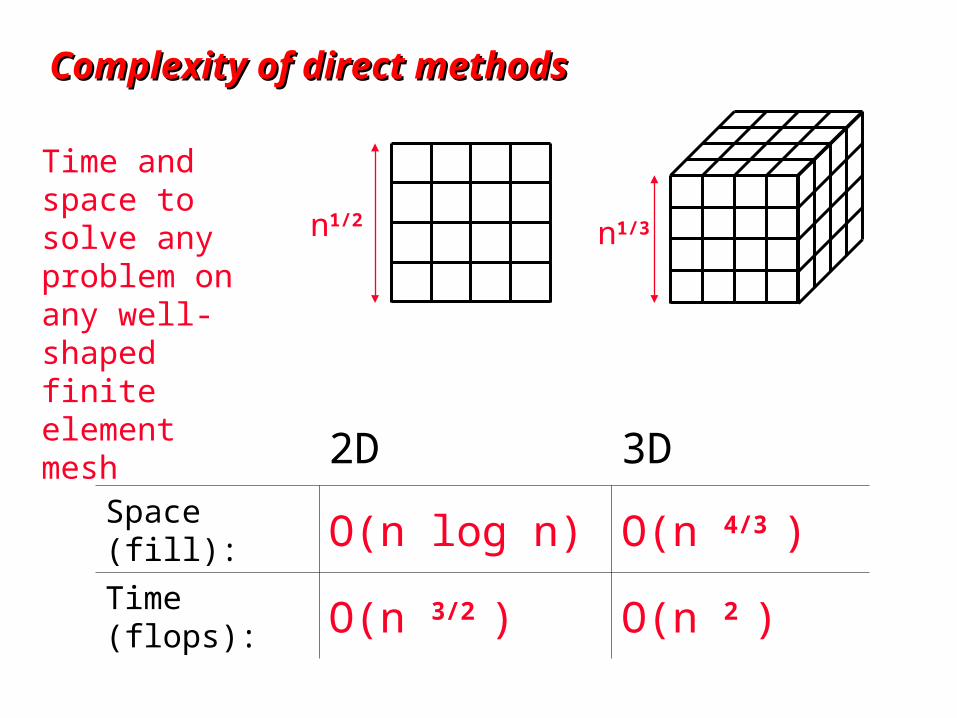
Complexity of direct methodsComplexity of direct methods
n1/2 n1/3
2D 3D
Space (fill): O(n log n) O(n 4/3 )
Time (flops): O(n 3/2 ) O(n 2 )
Time and space to solve any problem on any well-shaped finite element mesh
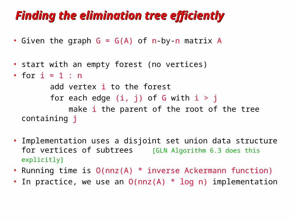
Finding the elimination tree efficientlyFinding the elimination tree efficiently
• Given the graph G = G(A) of n-by-n matrix A
• start with an empty forest (no vertices)• for i = 1 : n
add vertex i to the forest
for each edge (i, j) of G with i > j
make i the parent of the root of the tree containing j
• Implementation uses a disjoint set union data structure for vertices of subtrees [GLN Algorithm 6.3 does this explicitly]
• Running time is O(nnz(A) * inverse Ackermann function)• In practice, we use an O(nnz(A) * log n) implementation
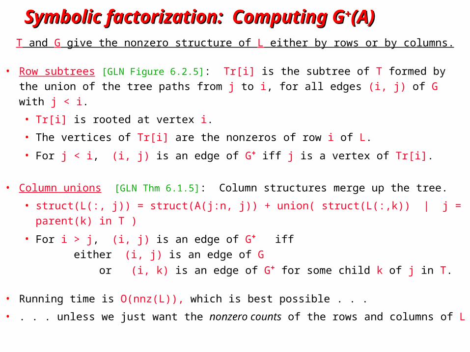
Symbolic factorization: Computing GSymbolic factorization: Computing G++(A)(A)
T and G give the nonzero structure of L either by rows or by columns.
• Row subtrees [GLN Figure 6.2.5]: Tr[i] is the subtree of T formed by
the union of the tree paths from j to i, for all edges (i, j) of G with j < i.
• Tr[i] is rooted at vertex i.
• The vertices of Tr[i] are the nonzeros of row i of L.
• For j < i, (i, j) is an edge of G+ iff j is a vertex of Tr[i].
• Column unions [GLN Thm 6.1.5]: Column structures merge up the tree.
• struct(L(:, j)) = struct(A(j:n, j)) + union( struct(L(:,k)) | j = parent(k) in T )
• For i > j, (i, j) is an edge of G+ iff
either (i, j) is an edge of G
or (i, k) is an edge of G+ for some child k of j in T.
• Running time is O(nnz(L)), which is best possible . . .
• . . . unless we just want the nonzero counts of the rows and columns of L

Finding row and column counts efficientlyFinding row and column counts efficiently
• First ingredient: number the elimination tree in postorder• Every subtree gets consecutive numbers• Renumbers vertices, but does not change fill or edges of G+
• Second ingredient: fast least-common-ancestor algorithm• lca (u, v) = root of smallest subtree containing both u and v• In a tree with n vertices, can do m arbitrary lca() computations
in time O(m * inverse Ackermann(m, n))• The fast lca algorithm uses a disjoint-set-union data structure
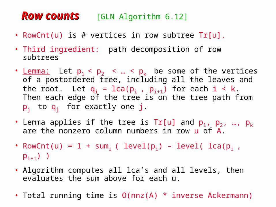
Row counts Row counts [GLN Algorithm 6.12]
• RowCnt(u) is # vertices in row subtree Tr[u].
• Third ingredient: path decomposition of row subtrees
• Lemma: Let p1 < p2 < … < pk be some of the vertices of a postordered tree, including all the leaves and the root. Let qi = lca(pi , pi+1) for each i < k. Then each edge of the tree is on the tree path from pj to qj for exactly one j.
• Lemma applies if the tree is Tr[u] and p1, p2, …, pk are the nonzero column numbers in row u of A.
• RowCnt(u) = 1 + sumi ( level(pi) – level( lca(pi , pi+1) )
• Algorithm computes all lca’s and all levels, then evaluates the sum above for each u.
• Total running time is O(nnz(A) * inverse Ackermann)
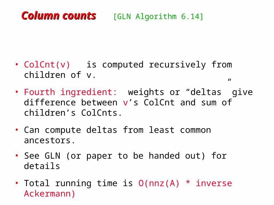
Column counts Column counts [GLN Algorithm 6.14]
• ColCnt(v) is computed recursively from children of v.
• Fourth ingredient: weights or “deltas” give difference between v’s ColCnt and sum of children’s ColCnts.
• Can compute deltas from least common ancestors.
• See GLN (or paper to be handed out) for details
• Total running time is O(nnz(A) * inverse Ackermann)
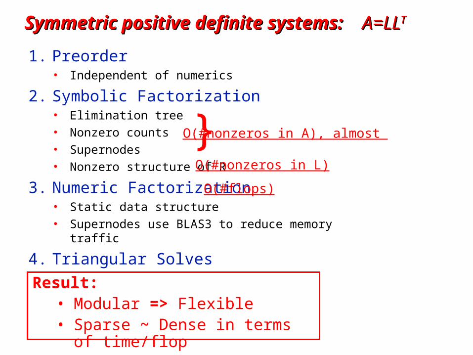
1. Preorder• Independent of numerics
2. Symbolic Factorization• Elimination tree
• Nonzero counts
• Supernodes
• Nonzero structure of R
3. Numeric Factorization• Static data structure
• Supernodes use BLAS3 to reduce memory traffic
4. Triangular Solves
Symmetric positive definite systems: Symmetric positive definite systems: A=LLA=LLTT
Result:• Modular => Flexible• Sparse ~ Dense in terms of time/flop
O(#flops)
O(#nonzeros in L)
}O(#nonzeros in A), almost
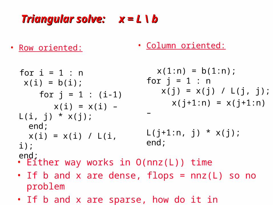
Triangular solve: x = L \ bTriangular solve: x = L \ b
• Row oriented:
for i = 1 : n x(i) = b(i);
for j = 1 : (i-1)
x(i) = x(i) – L(i, j) * x(j); end; x(i) = x(i) / L(i, i);end;
• Column oriented:
x(1:n) = b(1:n);for j = 1 : n x(j) = x(j) / L(j, j);
x(j+1:n) = x(j+1:n) – L(j+1:n, j) * x(j); end;
• Either way works in O(nnz(L)) time • If b and x are dense, flops = nnz(L) so no problem• If b and x are sparse, how do it in O(flops) time?

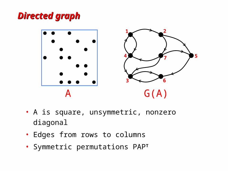
Directed GraphDirected Graph
• A is square, unsymmetric, nonzero diagonal
• Edges from rows to columns
• Symmetric permutations PAPT
1 2
3
4 7
6
5
A G(A)
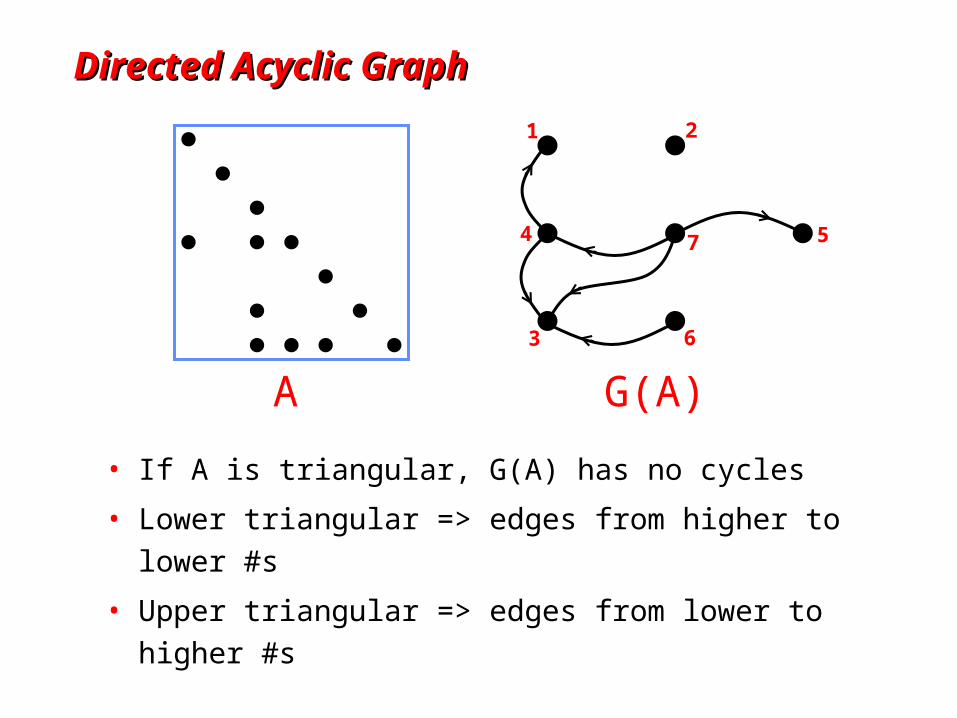
Directed Acyclic GraphDirected Acyclic Graph
• If A is triangular, G(A) has no cycles
• Lower triangular => edges from higher to lower #s
• Upper triangular => edges from lower to higher #s
1 2
3
4 7
6
5
A G(A)
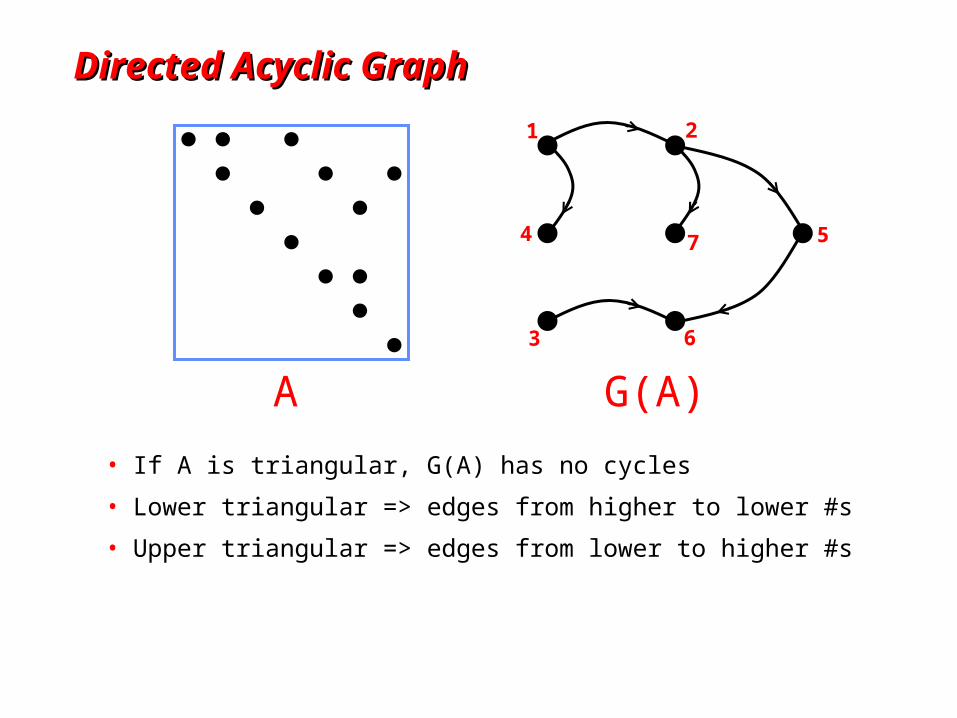
Directed Acyclic GraphDirected Acyclic Graph
• If A is triangular, G(A) has no cycles
• Lower triangular => edges from higher to lower #s
• Upper triangular => edges from lower to higher #s
1 2
3
4 7
6
5
A G(A)
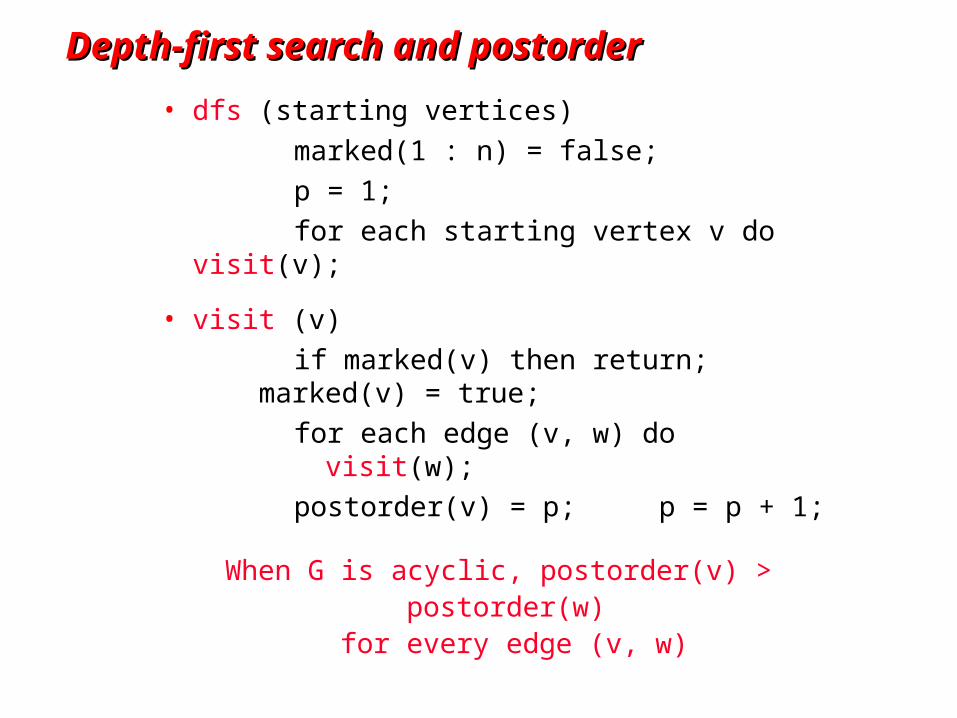
Depth-first search and postorderDepth-first search and postorder
• dfs (starting vertices)
marked(1 : n) = false;
p = 1;
for each starting vertex v do visit(v);
• visit (v)
if marked(v) then return; marked(v) = true;
for each edge (v, w) do visit(w);
postorder(v) = p; p = p + 1;
When G is acyclic, postorder(v) > postorder(w) for every edge (v, w)
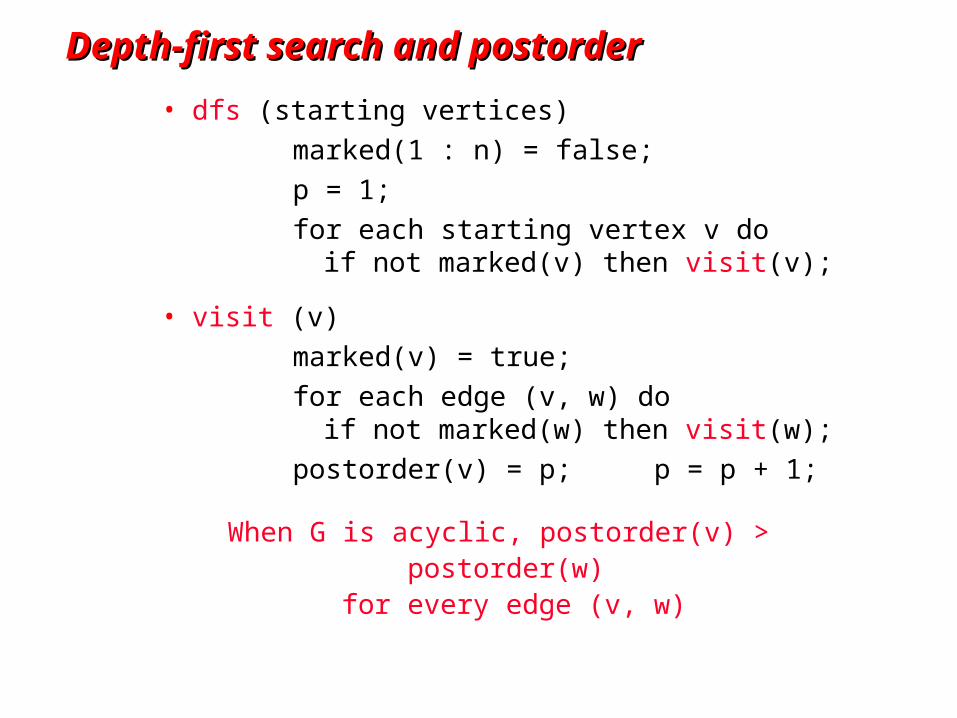
Depth-first search and postorderDepth-first search and postorder
• dfs (starting vertices)
marked(1 : n) = false;
p = 1;
for each starting vertex v do if not marked(v) then visit(v);
• visit (v)
marked(v) = true;
for each edge (v, w) do if not marked(w) then visit(w);
postorder(v) = p; p = p + 1;
When G is acyclic, postorder(v) > postorder(w) for every edge (v, w)
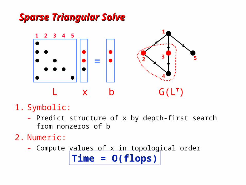
Sparse Triangular SolveSparse Triangular Solve
1 52 3 4
=
G(LT)
1
2 3
4
5
L x b
1. Symbolic:– Predict structure of x by depth-first search from nonzeros of b
2. Numeric:– Compute values of x in topological order
Time = O(flops)
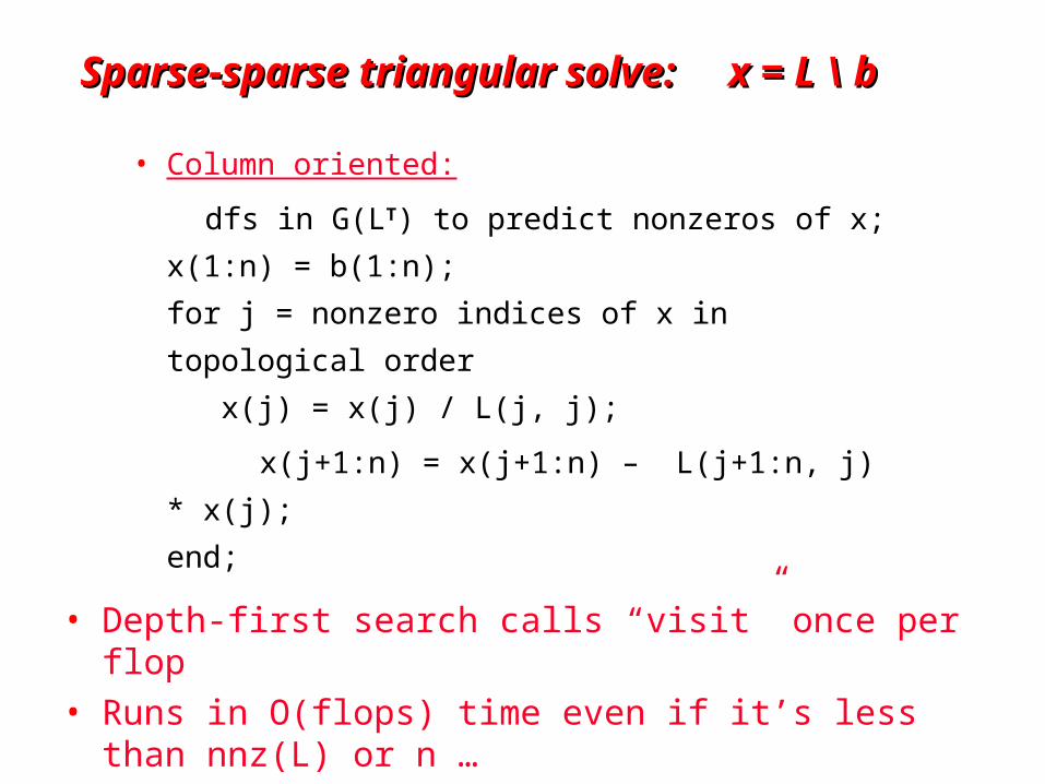
Sparse-sparse triangular solve: x = L \ bSparse-sparse triangular solve: x = L \ b
• Column oriented:
dfs in G(LT) to predict nonzeros of x;
x(1:n) = b(1:n);
for j = nonzero indices of x in topological order
x(j) = x(j) / L(j, j);
x(j+1:n) = x(j+1:n) – L(j+1:n, j) * x(j);
end;
• Depth-first search calls “visit” once per flop• Runs in O(flops) time even if it’s less than nnz(L) or n …• Except for one-time O(n) SPA setup
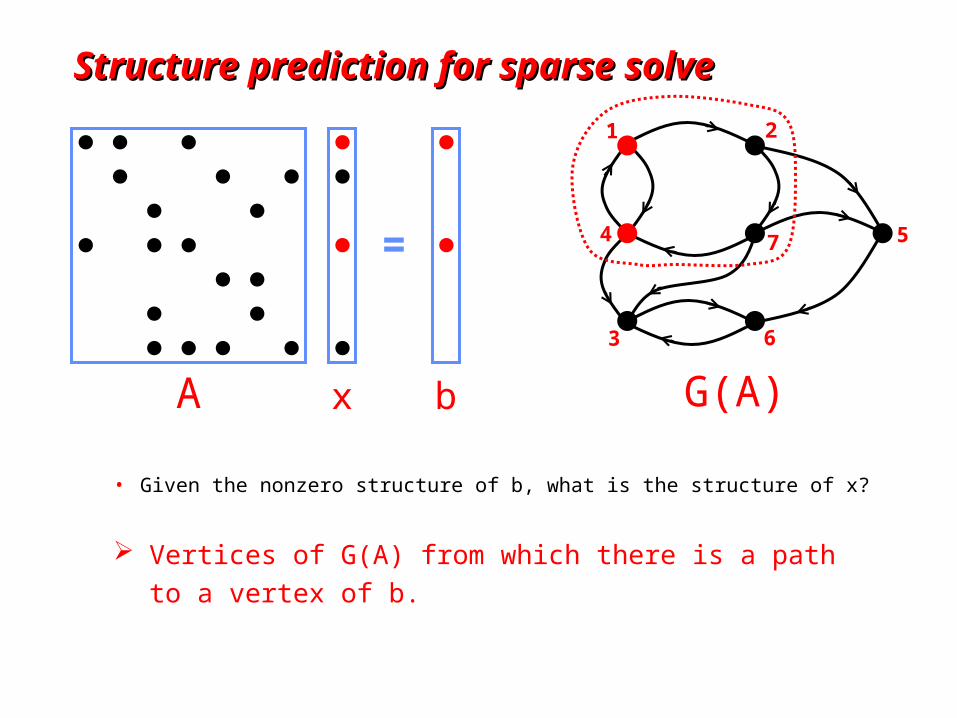
Structure prediction for sparse solveStructure prediction for sparse solve
• Given the nonzero structure of b, what is the structure of x?
A G(A) x b
=
1 2
3
4 7
6
5
Vertices of G(A) from which there is a path to a vertex of b.
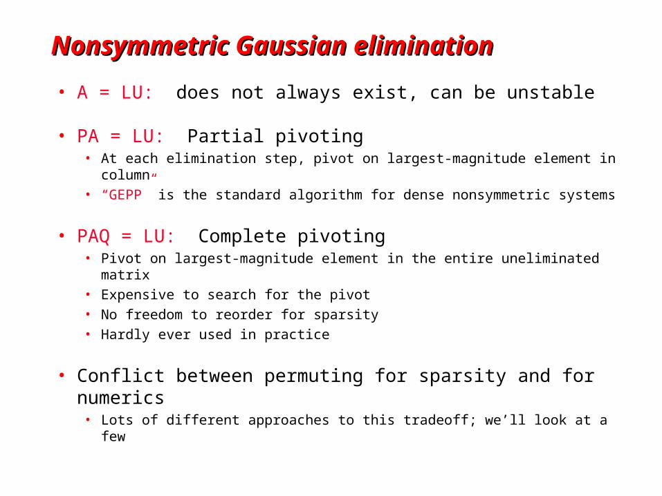
Nonsymmetric Gaussian eliminationNonsymmetric Gaussian elimination
• A = LU: does not always exist, can be unstable
• PA = LU: Partial pivoting• At each elimination step, pivot on largest-magnitude element in column
• “GEPP” is the standard algorithm for dense nonsymmetric systems
• PAQ = LU: Complete pivoting• Pivot on largest-magnitude element in the entire uneliminated matrix
• Expensive to search for the pivot
• No freedom to reorder for sparsity
• Hardly ever used in practice
• Conflict between permuting for sparsity and for numerics• Lots of different approaches to this tradeoff; we’ll look at a few
+
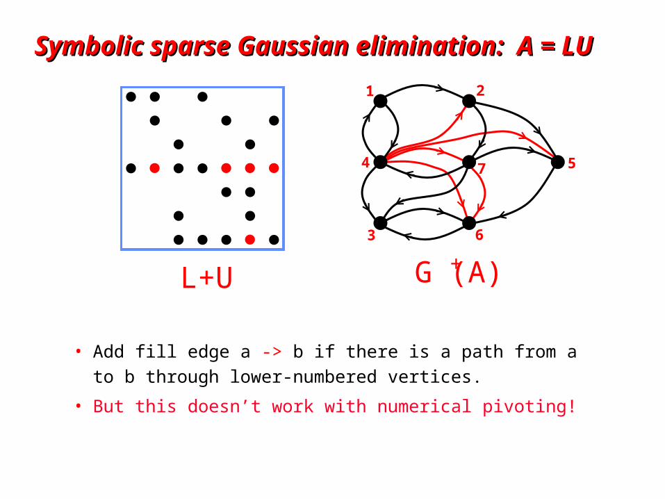
Symbolic sparse Gaussian elimination: A = LUSymbolic sparse Gaussian elimination: A = LU
• Add fill edge a -> b if there is a path from a to b
through lower-numbered vertices.
• But this doesn’t work with numerical pivoting!
1 2
3
4 7
6
5
A G (A) L+U
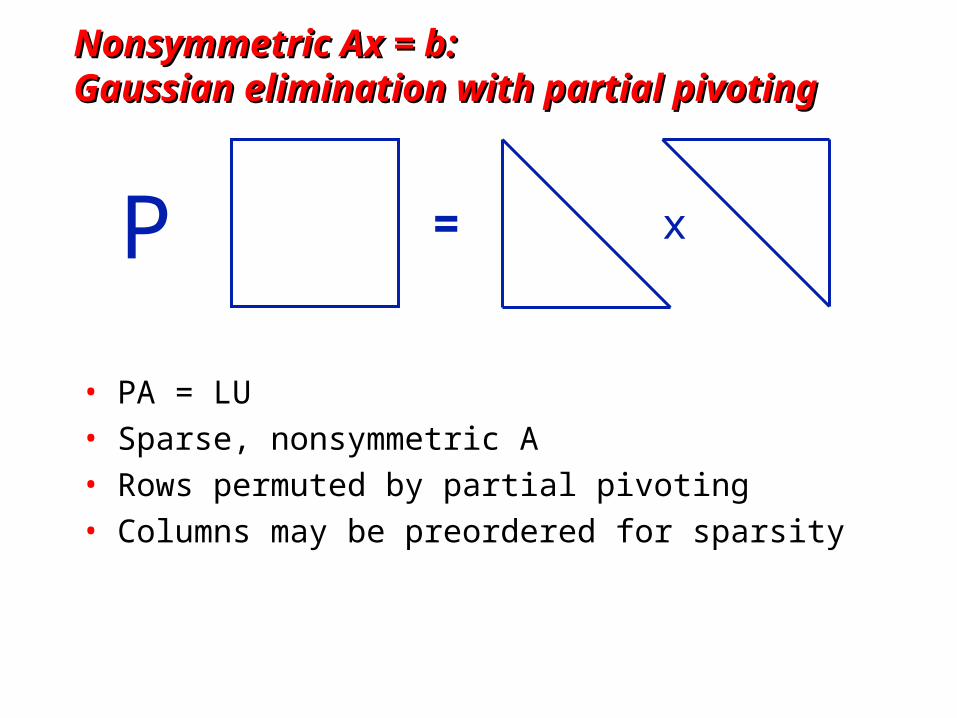
Nonsymmetric Ax = b: Nonsymmetric Ax = b: Gaussian elimination with partial pivotingGaussian elimination with partial pivoting
• PA = LU• Sparse, nonsymmetric A• Rows permuted by partial pivoting• Columns may be preordered for sparsity
= xP
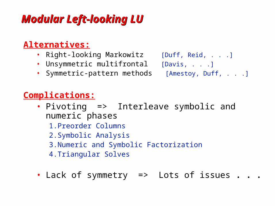
Modular Left-looking LUModular Left-looking LU
Alternatives:• Right-looking Markowitz [Duff, Reid, . . .]
• Unsymmetric multifrontal [Davis, . . .]
• Symmetric-pattern methods [Amestoy, Duff, . . .]
Complications:• Pivoting => Interleave symbolic and numeric phases
1. Preorder Columns2. Symbolic Analysis3. Numeric and Symbolic Factorization4. Triangular Solves
• Lack of symmetry => Lots of issues . . .
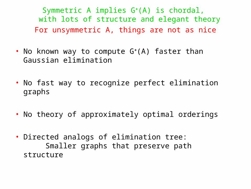
Symmetric A implies G+(A) is chordal, with lots of structure and elegant theory
For unsymmetric A, things are not as nice
• No known way to compute G+(A) faster than Gaussian elimination
• No fast way to recognize perfect elimination graphs
• No theory of approximately optimal orderings
• Directed analogs of elimination tree: Smaller graphs that preserve path structure

Left-looking Column LU FactorizationLeft-looking Column LU Factorization
for column j = 1 to n do
solve
pivot: swap ujj and an elt of lj
scale: lj = lj / ujj
• Column j of A becomes column j of L and U
L 0L I( ) uj
lj ( ) = aj for uj, lj
L
LU
A
j
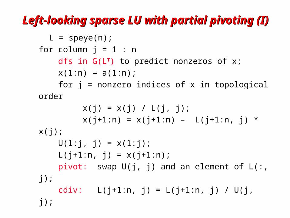
Left-looking sparse LU with partial pivoting (I)Left-looking sparse LU with partial pivoting (I)
L = speye(n);
for column j = 1 : n
dfs in G(LT) to predict nonzeros of x;
x(1:n) = a(1:n);
for j = nonzero indices of x in topological order
x(j) = x(j) / L(j, j);
x(j+1:n) = x(j+1:n) – L(j+1:n, j) * x(j);
U(1:j, j) = x(1:j);
L(j+1:n, j) = x(j+1:n);
pivot: swap U(j, j) and an element of L(:, j);
cdiv: L(j+1:n, j) = L(j+1:n, j) / U(j, j);
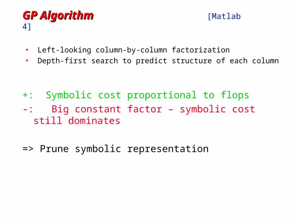
GP AlgorithmGP Algorithm [Matlab 4]
• Left-looking column-by-column factorization• Depth-first search to predict structure of each column
+: Symbolic cost proportional to flops
-: Big constant factor – symbolic cost still dominates
=> Prune symbolic representation
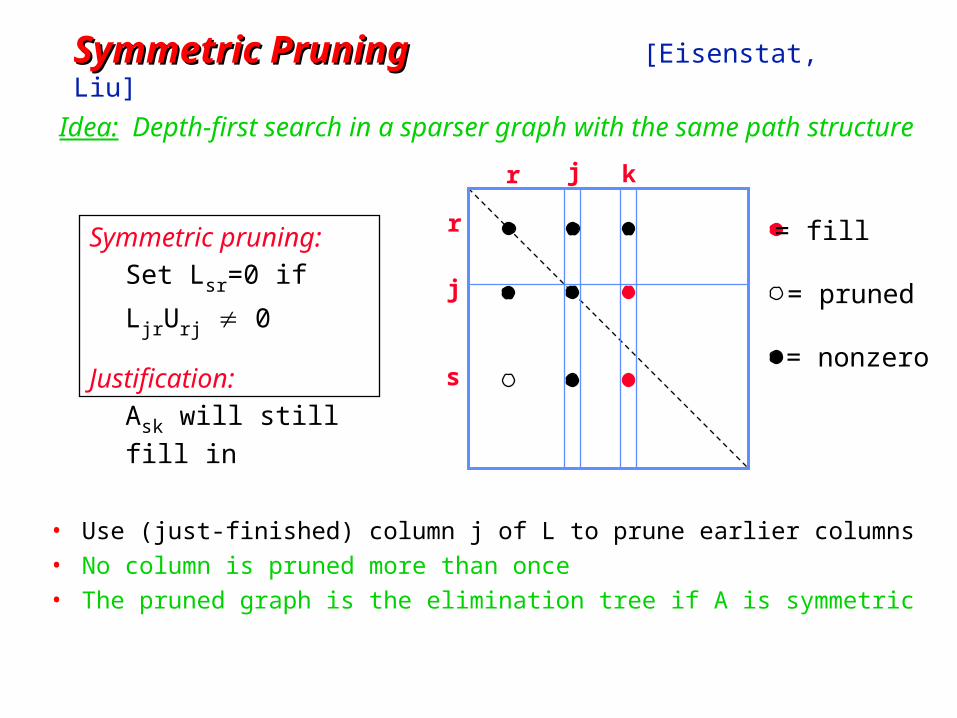
Symmetric Pruning Symmetric Pruning [Eisenstat, Liu]
• Use (just-finished) column j of L to prune earlier columns• No column is pruned more than once• The pruned graph is the elimination tree if A is symmetric
Idea: Depth-first search in a sparser graph with the same path structure
Symmetric pruning:
Set Lsr=0 if LjrUrj 0
Justification:
Ask will still fill in
r
r j
j
s
k
= fill
= pruned
= nonzero
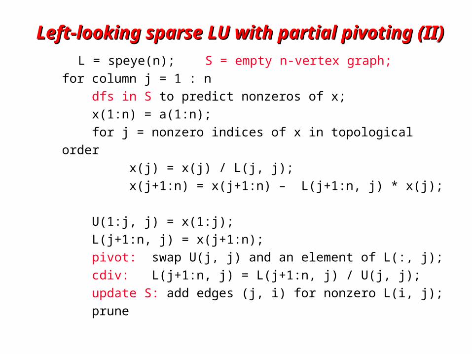
Left-looking sparse LU with partial pivoting (II)Left-looking sparse LU with partial pivoting (II)
L = speye(n); S = empty n-vertex graph;
for column j = 1 : n
dfs in S to predict nonzeros of x;
x(1:n) = a(1:n);
for j = nonzero indices of x in topological order
x(j) = x(j) / L(j, j);
x(j+1:n) = x(j+1:n) – L(j+1:n, j) * x(j);
U(1:j, j) = x(1:j);
L(j+1:n, j) = x(j+1:n);
pivot: swap U(j, j) and an element of L(:, j);
cdiv: L(j+1:n, j) = L(j+1:n, j) / U(j, j);
update S: add edges (j, i) for nonzero L(i, j);
prune
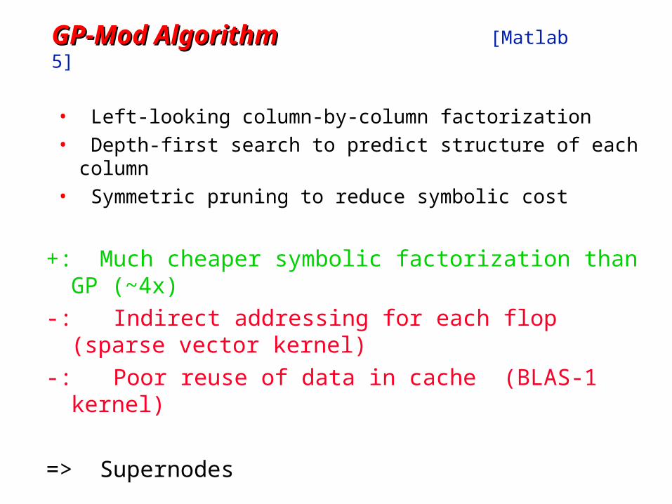
GP-Mod Algorithm GP-Mod Algorithm [Matlab 5]
• Left-looking column-by-column factorization• Depth-first search to predict structure of each column• Symmetric pruning to reduce symbolic cost
+: Much cheaper symbolic factorization than GP (~4x)
-: Indirect addressing for each flop (sparse vector kernel)
-: Poor reuse of data in cache (BLAS-1 kernel)
=> Supernodes
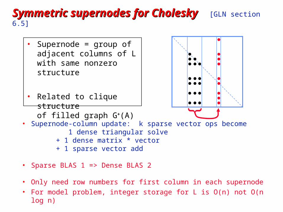
Symmetric supernodes for Cholesky Symmetric supernodes for Cholesky [GLN section 6.5]
• Supernode-column update: k sparse vector ops become 1 dense triangular solve+ 1 dense matrix * vector+ 1 sparse vector add
• Sparse BLAS 1 => Dense BLAS 2
• Only need row numbers for first column in each supernode• For model problem, integer storage for L is O(n) not O(n log n)
{
• Supernode = group of adjacent columns of L with same nonzero structure
• Related to clique structureof filled graph G+(A)
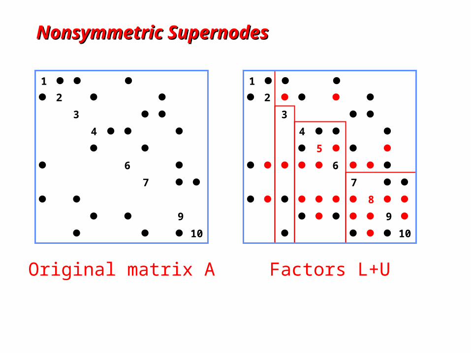
Nonsymmetric SupernodesNonsymmetric Supernodes
1
2
3
4
5
6
10
7
8
9
Original matrix A Factors L+U
1
2
3
4
5
6
10
7
8
9
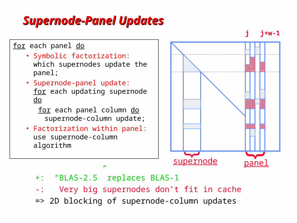
Supernode-Panel UpdatesSupernode-Panel Updates
for each panel do
• Symbolic factorization: which supernodes update the panel;
• Supernode-panel update: for each updating supernode do
for each panel column do supernode-column update;
• Factorization within panel: use supernode-column algorithm
+: “BLAS-2.5” replaces BLAS-1
-: Very big supernodes don’t fit in cache
=> 2D blocking of supernode-column updates
j j+w-1
supernode panel
} }
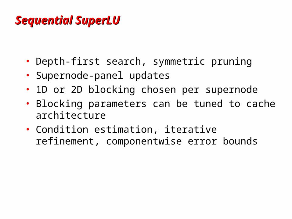
Sequential SuperLUSequential SuperLU
• Depth-first search, symmetric pruning• Supernode-panel updates• 1D or 2D blocking chosen per supernode• Blocking parameters can be tuned to cache architecture• Condition estimation, iterative refinement,
componentwise error bounds
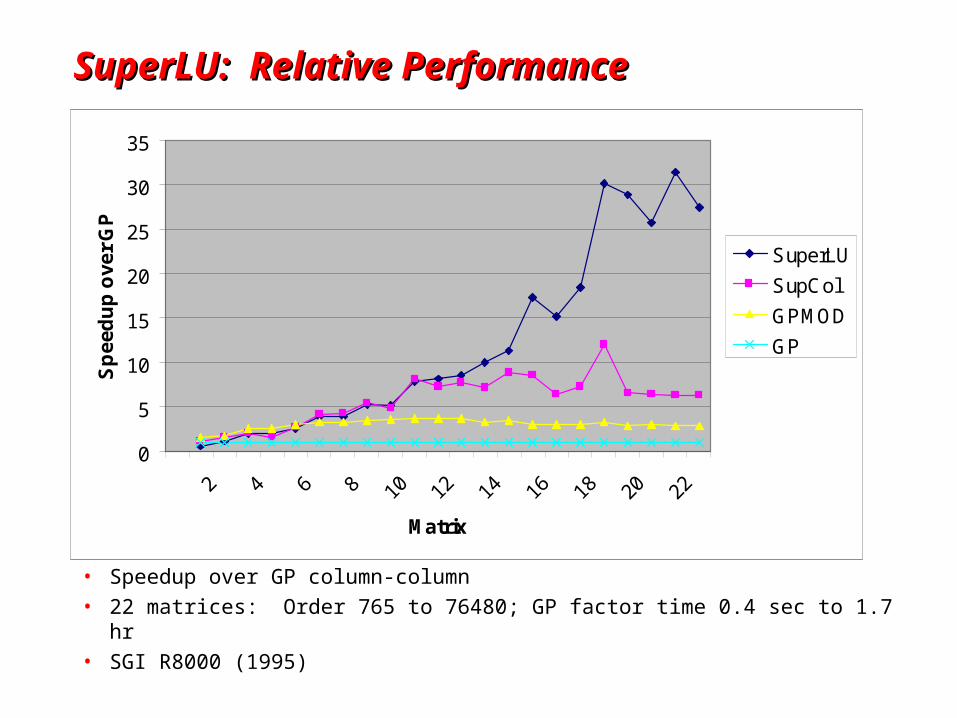
SuperLU: Relative PerformanceSuperLU: Relative Performance
• Speedup over GP column-column• 22 matrices: Order 765 to 76480; GP factor time 0.4 sec to 1.7 hr• SGI R8000 (1995)
0
5
10
15
20
25
30
35
Matrix
Sp
eed
up
ove
r G
P
SuperLU
SupCol
GPMOD
GP

Nonsymmetric Ax = b: Nonsymmetric Ax = b: Gaussian elimination with partial pivotingGaussian elimination with partial pivoting
• PA = LU• Sparse, nonsymmetric A• Rows permuted by partial pivoting• Columns may be preordered for sparsity
= xP
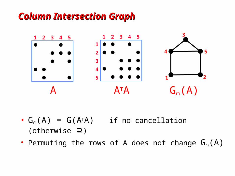
Column Intersection GraphColumn Intersection Graph
• G(A) = G(ATA) if no cancellation (otherwise )
• Permuting the rows of A does not change G(A)
1 52 3 4
1 2
3
4 5
1 52 3 4
1
5
2
3
4
A G(A) ATA
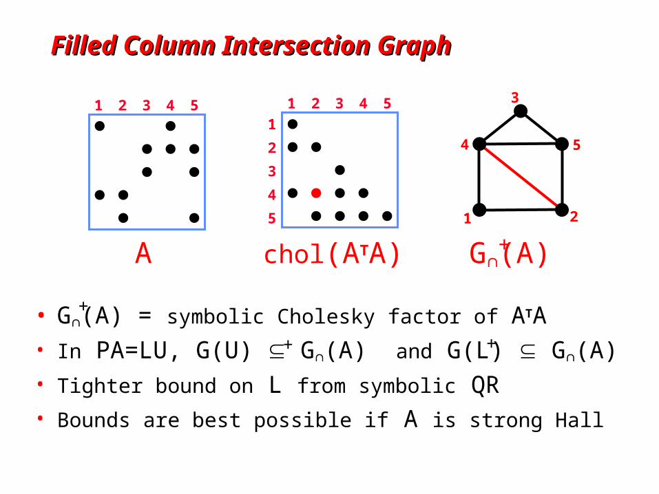
Filled Column Intersection GraphFilled Column Intersection Graph
• G(A) = symbolic Cholesky factor of ATA• In PA=LU, G(U) G(A) and G(L) G(A)• Tighter bound on L from symbolic QR • Bounds are best possible if A is strong Hall
1 52 3 4
1 2
3
4 5
A
1 52 3 4
1
5
2
3
4
chol(ATA) G(A) +
+
++
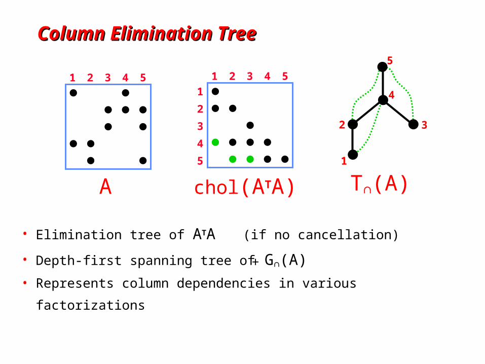
Column Elimination TreeColumn Elimination Tree
• Elimination tree of ATA (if no cancellation)
• Depth-first spanning tree of G(A)
• Represents column dependencies in various factorizations
1 52 3 4
1
5
4
2 3
A
1 52 3 4
1
5
2
3
4
chol(ATA) T(A)
+
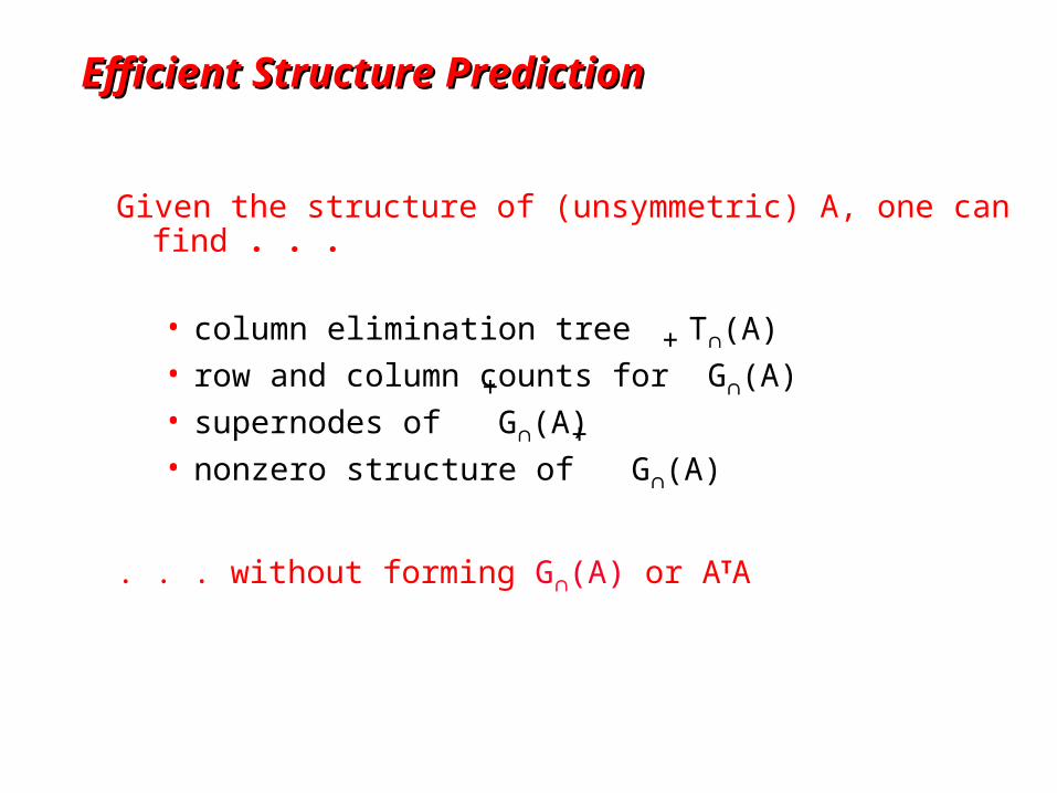
Efficient Structure PredictionEfficient Structure Prediction
Given the structure of (unsymmetric) A, one can find . . .
• column elimination tree T(A)• row and column counts for G(A)• supernodes of G(A)• nonzero structure of G(A)
. . . without forming G(A) or ATA
+
+
+
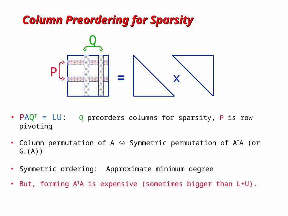
Column Preordering for SparsityColumn Preordering for Sparsity
• PAQT = LU: Q preorders columns for sparsity, P is row pivoting
• Column permutation of A Symmetric permutation of ATA (or G(A))
• Symmetric ordering: Approximate minimum degree
• But, forming ATA is expensive (sometimes bigger than L+U).
= xP
Q
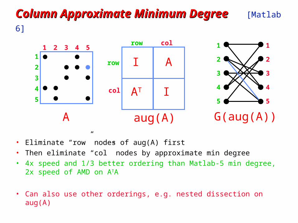
Column Approximate Minimum Degree Column Approximate Minimum Degree [Matlab 6]
• Eliminate “row” nodes of aug(A) first• Then eliminate “col” nodes by approximate min degree• 4x speed and 1/3 better ordering than Matlab-5 min degree,
2x speed of AMD on ATA
• Can also use other orderings, e.g. nested dissection on aug(A)
1 52 3 41
5
2
3
4
A
A
AT I
I
row
row
col
col
aug(A) G(aug(A))
1
5
2
3
4
1
5
2
3
4

Column Elimination TreeColumn Elimination Tree
• Elimination tree of ATA (if no cancellation)
• Depth-first spanning tree of G(A)
• Represents column dependencies in various factorizations
1 52 3 4
1
5
4
2 3
A
1 52 3 4
1
5
2
3
4
chol(ATA) T(A)
+
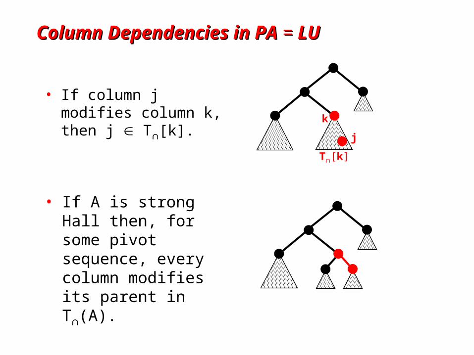
Column Dependencies in PA Column Dependencies in PA == LU LU
• If column j modifies column k, then j T[k].
k
j
T[k]
• If A is strong Hall then, for some pivot sequence, every column modifies its parent in T(A).
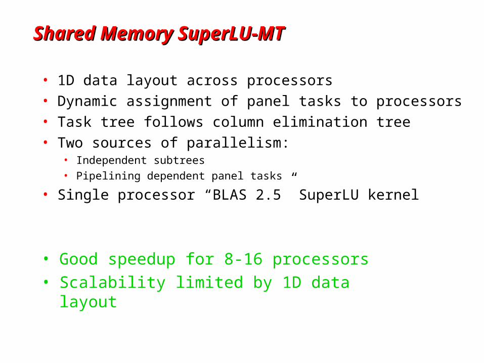
Shared Memory SuperLU-MTShared Memory SuperLU-MT
• 1D data layout across processors• Dynamic assignment of panel tasks to processors• Task tree follows column elimination tree• Two sources of parallelism:
• Independent subtrees
• Pipelining dependent panel tasks
• Single processor “BLAS 2.5” SuperLU kernel
• Good speedup for 8-16 processors• Scalability limited by 1D data layout
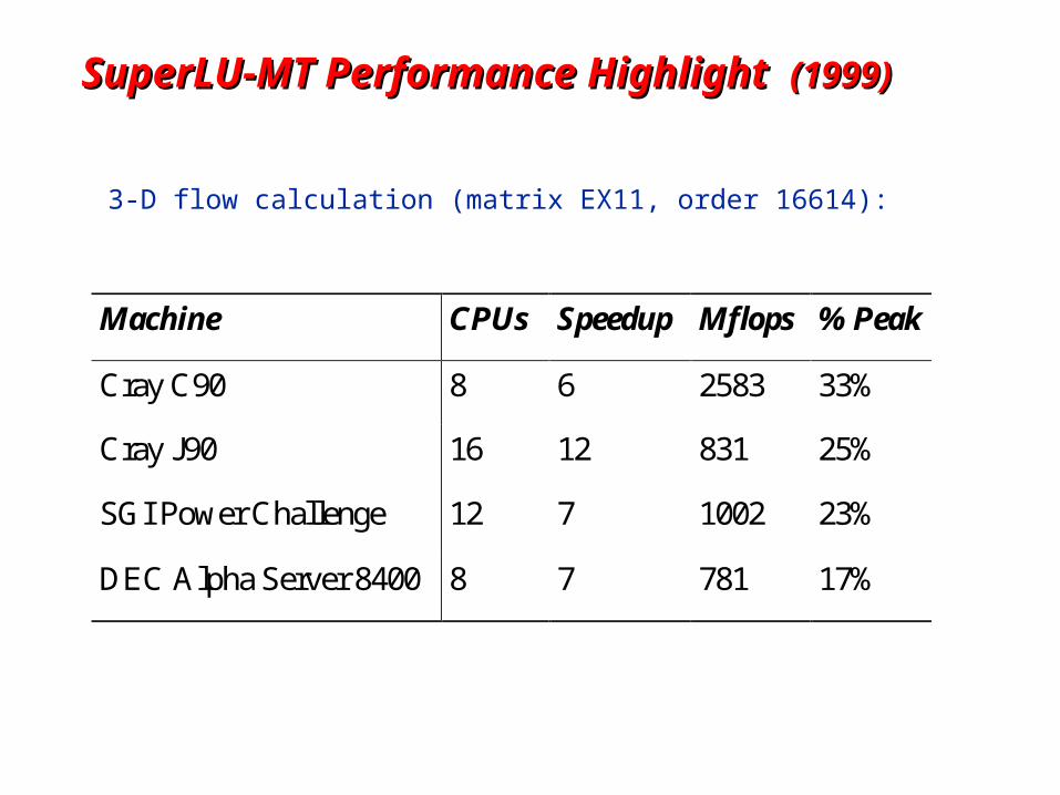
SuperLU-MT Performance Highlight SuperLU-MT Performance Highlight (1999)(1999)
3-D flow calculation (matrix EX11, order 16614):
Machine CPUs Speedup Mflops % Peak
Cray C90 8 6 2583 33%
Cray J90 16 12 831 25%
SGI Power Challenge 12 7 1002 23%
DEC Alpha Server 8400 8 7 781 17%
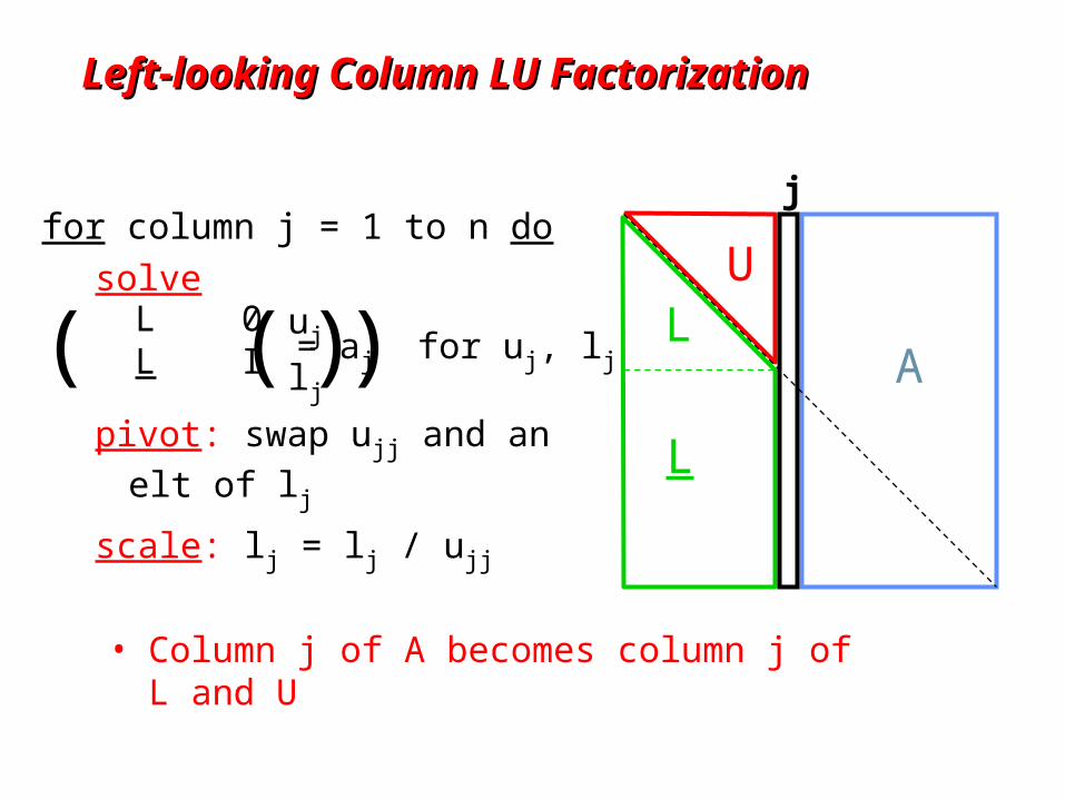
Left-looking Column LU FactorizationLeft-looking Column LU Factorization
for column j = 1 to n do
solve
pivot: swap ujj and an elt of lj
scale: lj = lj / ujj
• Column j of A becomes column j of L and U
L 0L I( ) uj
lj ( ) = aj for uj, lj
L
LU
A
j
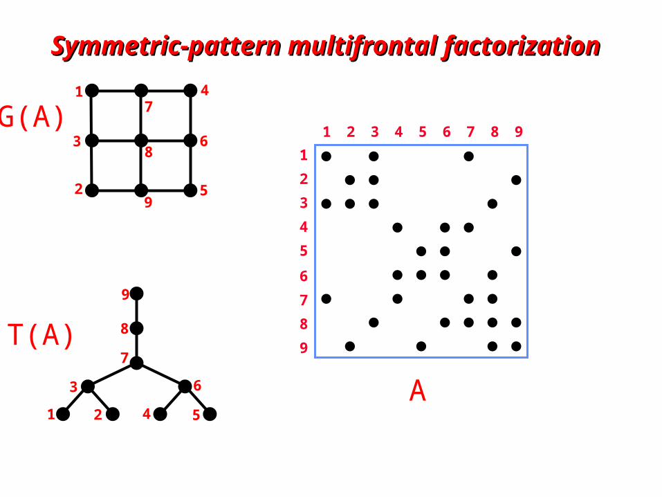
Symmetric-pattern multifrontal factorizationSymmetric-pattern multifrontal factorization
T(A)
1 2
3
4
6
7
8
9
5
5 96 7 81 2 3 4
1
5
2
3
4
9
6
7
8
A
9
1
2
3
4
6
7
8
5
G(A)
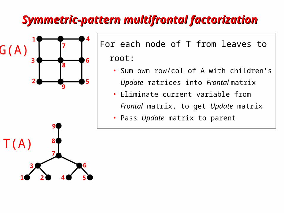
Symmetric-pattern multifrontal factorizationSymmetric-pattern multifrontal factorization
T(A)
1 2
3
4
6
7
8
9
5
For each node of T from leaves to root:• Sum own row/col of A with children’s
Update matrices into Frontal matrix
• Eliminate current variable from Frontal
matrix, to get Update matrix
• Pass Update matrix to parent
9
1
2
3
4
6
7
8
5
G(A)
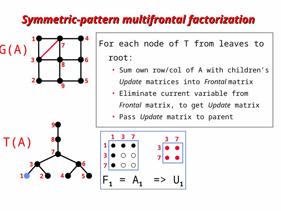
Symmetric-pattern multifrontal factorizationSymmetric-pattern multifrontal factorization
T(A)
1 2
3
4
6
7
8
9
5
1 3 71
3
7
3 73
7
F1 = A1 => U1
For each node of T from leaves to root:• Sum own row/col of A with children’s
Update matrices into Frontal matrix
• Eliminate current variable from Frontal
matrix, to get Update matrix
• Pass Update matrix to parent
9
1
2
3
4
6
7
8
5
G(A)
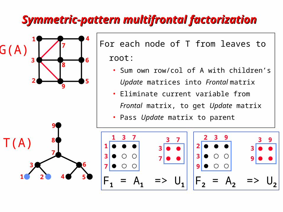
Symmetric-pattern multifrontal factorizationSymmetric-pattern multifrontal factorization
2 3 92
3
9
3 93
9
F2 = A2 => U2
1 3 71
3
7
3 73
7
F1 = A1 => U1
For each node of T from leaves to root:• Sum own row/col of A with children’s
Update matrices into Frontal matrix
• Eliminate current variable from Frontal
matrix, to get Update matrix
• Pass Update matrix to parent
T(A)
1 2
3
4
6
7
8
9
5
9
1
2
3
4
6
7
8
5
G(A)
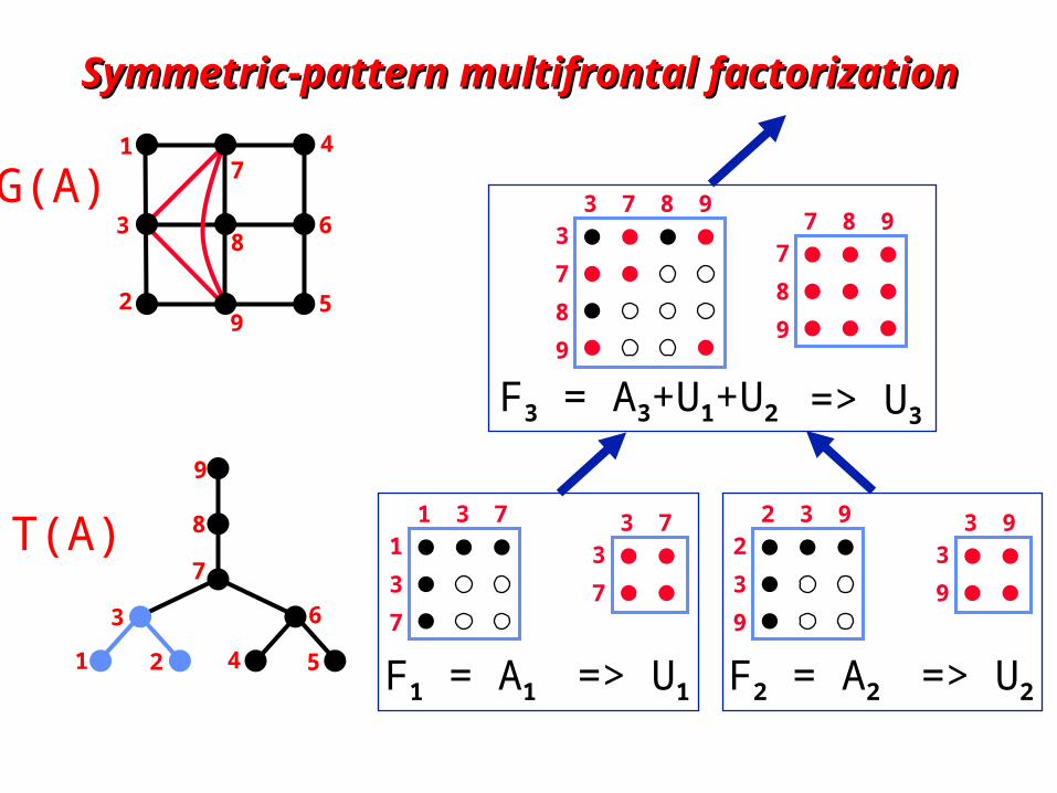
Symmetric-pattern multifrontal factorizationSymmetric-pattern multifrontal factorization
T(A) 2 3 9
2
3
9
3 93
9
F2 = A2 => U2
1 3 71
3
7
3 73
7
F1 = A1 => U1
3 7 8 93
7
8
9
7 8 97
8
9
F3 = A3+U1+U2 => U3
1 2
3
4
6
7
8
9
5
9
1
2
3
4
6
7
8
5
G(A)
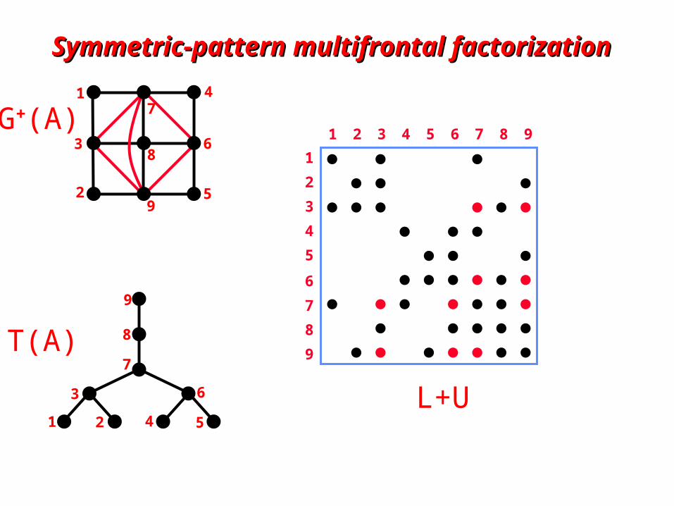
Symmetric-pattern multifrontal factorizationSymmetric-pattern multifrontal factorization
T(A)
1 2
3
4
6
7
8
9
5
5 96 7 81 2 3 4
1
5
2
3
4
9
6
7
8
L+U
9
1
2
3
4
6
7
8
5
G+(A)
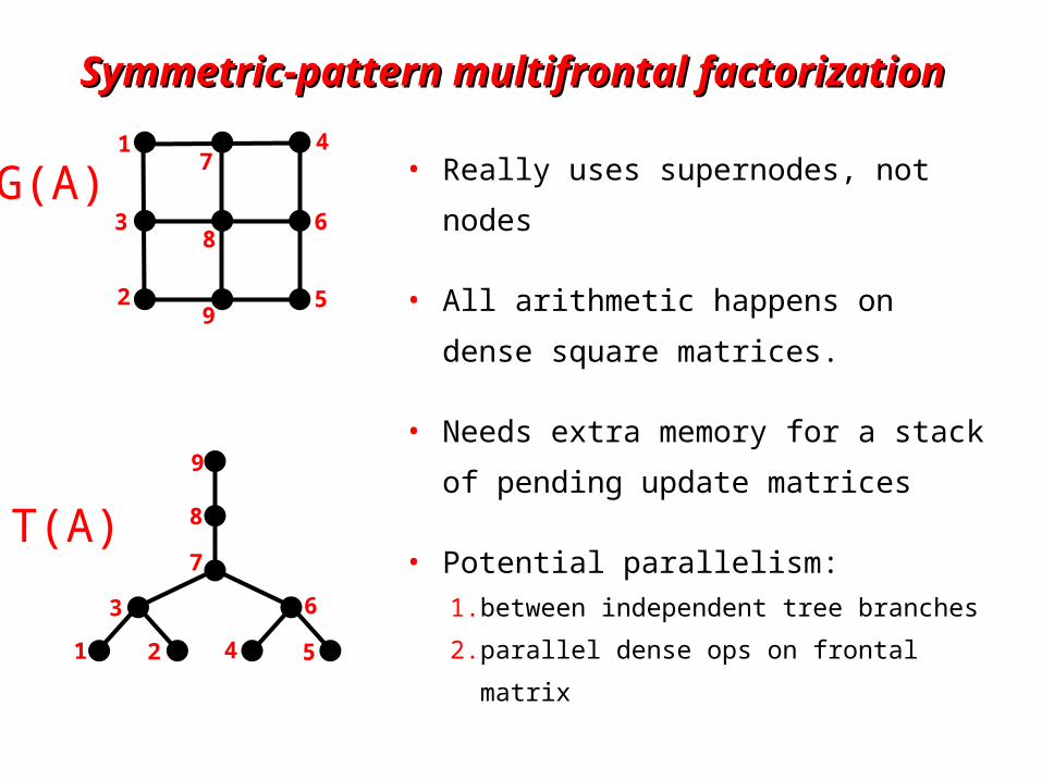
Symmetric-pattern multifrontal factorizationSymmetric-pattern multifrontal factorization
T(A)
1 2
3
4
6
7
8
9
5
1
2
3
4
6
7
8
95
G(A) • Really uses supernodes, not nodes
• All arithmetic happens on
dense square matrices.
• Needs extra memory for a stack of
pending update matrices
• Potential parallelism:
1. between independent tree branches
2. parallel dense ops on frontal matrix
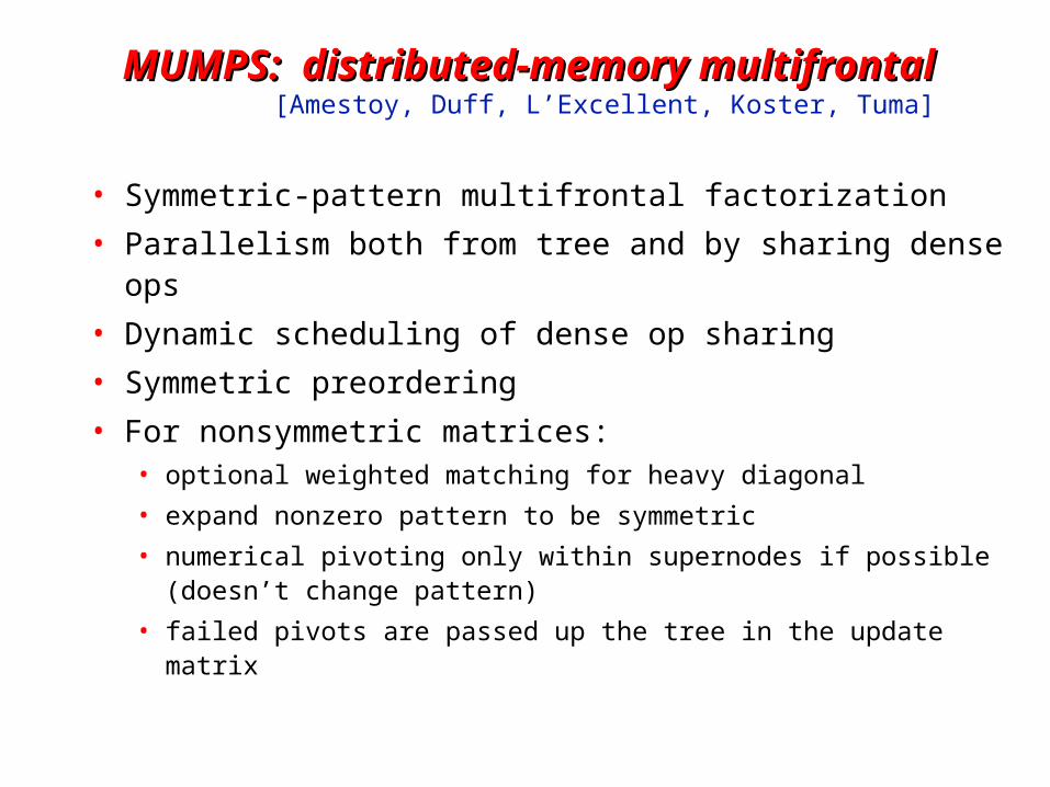
MUMPS: distributed-memory multifrontalMUMPS: distributed-memory multifrontal[Amestoy, Duff, L’Excellent, Koster, Tuma]
• Symmetric-pattern multifrontal factorization
• Parallelism both from tree and by sharing dense ops
• Dynamic scheduling of dense op sharing
• Symmetric preordering
• For nonsymmetric matrices:• optional weighted matching for heavy diagonal
• expand nonzero pattern to be symmetric
• numerical pivoting only within supernodes if possible (doesn’t change pattern)
• failed pivots are passed up the tree in the update matrix
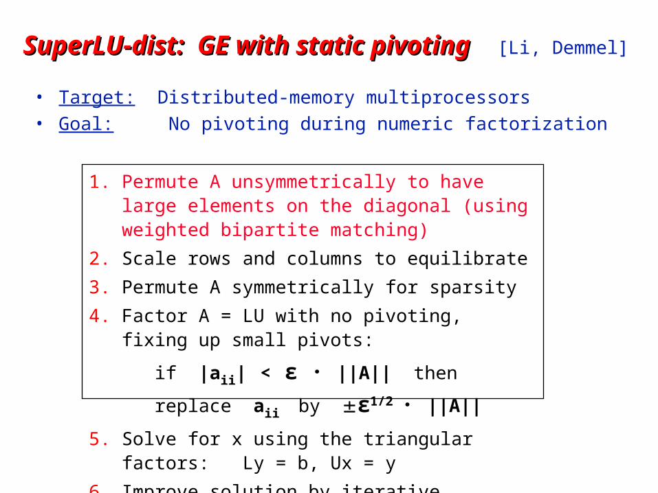
SuperLU-dist: GE with static pivoting SuperLU-dist: GE with static pivoting [Li, Demmel]
• Target: Distributed-memory multiprocessors
• Goal: No pivoting during numeric factorization
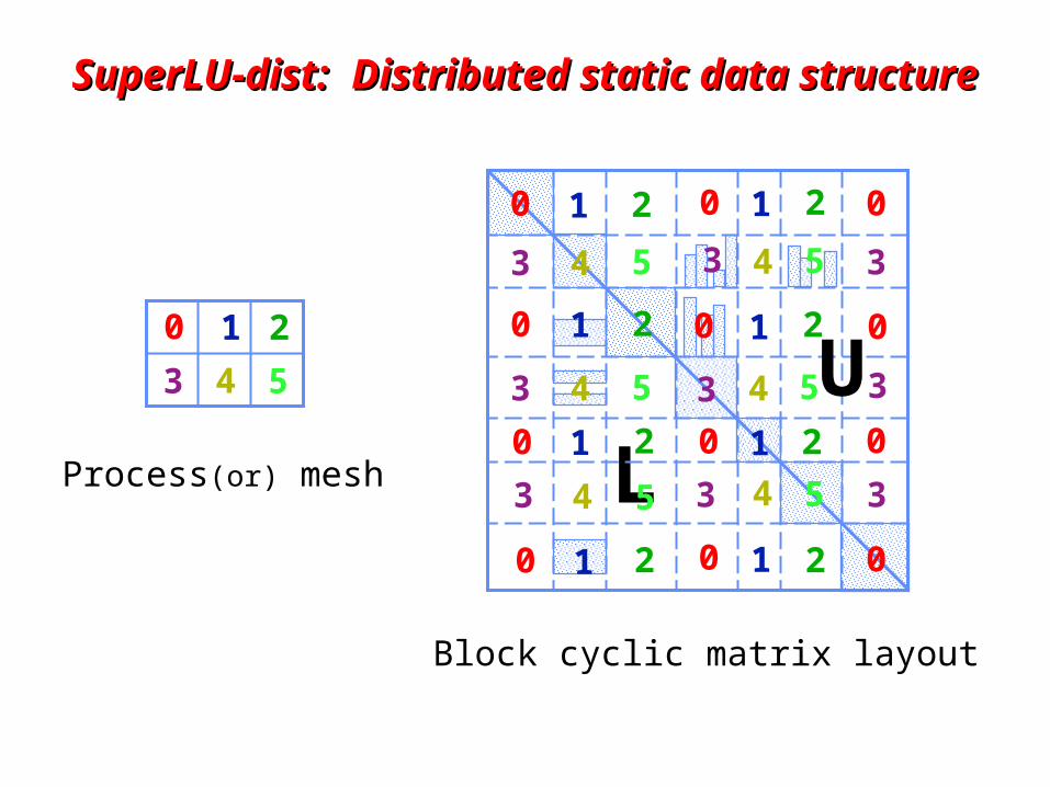
SuperLU-dist: SuperLU-dist: Distributed static data structureDistributed static data structure
Process(or) mesh
0 1 2
3 4 5
L0
0 1 2
3 4 5
0 1 2
3 4 5
0 1 2
3 4 5
0 1 2
3 4 5
0 1 2
3 4 5
0 1 2
0 1 2
3 4 5
0 1 2
0
3
0
3
0
3
U
Block cyclic matrix layout
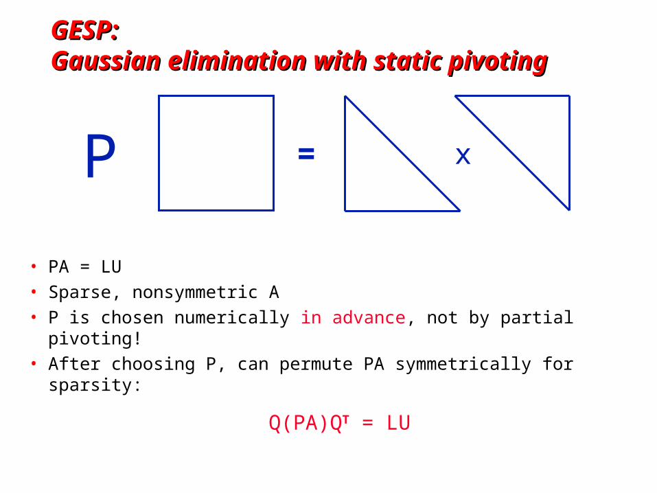
GESP: GESP: Gaussian elimination with static pivotingGaussian elimination with static pivoting
• PA = LU• Sparse, nonsymmetric A• P is chosen numerically in advance, not by partial pivoting!• After choosing P, can permute PA symmetrically for sparsity:
Q(PA)QT = LU
= xP
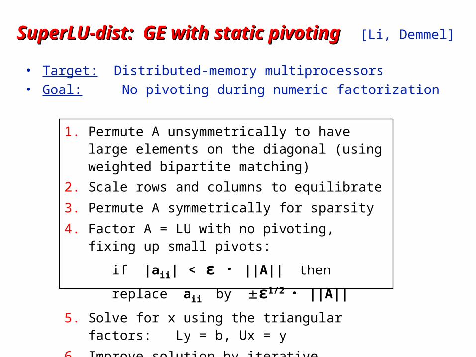
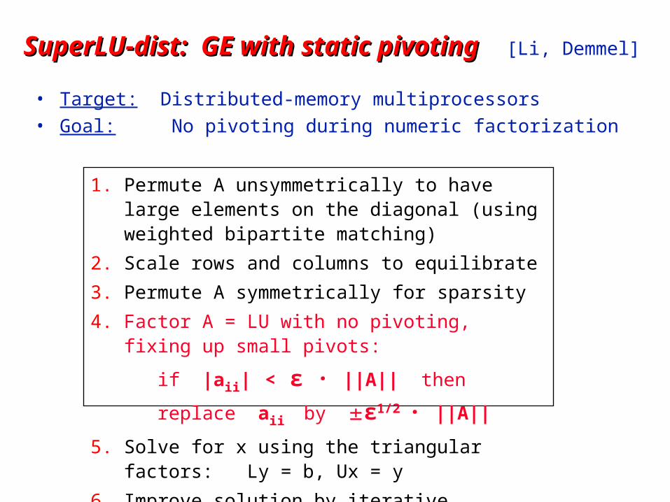
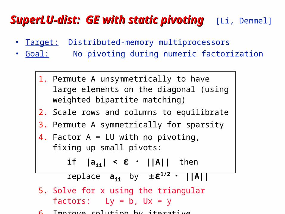
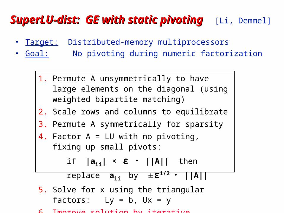
SuperLU-dist: GE with static pivoting SuperLU-dist: GE with static pivoting [Li, Demmel]
• Target: Distributed-memory multiprocessors• Goal: No pivoting during numeric factorization
1. Permute A unsymmetrically to have large elements on the diagonal (using weighted bipartite matching)
2. Scale rows and columns to equilibrate
3. Permute A symmetrically for sparsity
4. Factor A = LU with no pivoting, fixing up small pivots:
if |aii| < ε · ||A|| then replace aii by ε1/2 · ||A||
5. Solve for x using the triangular factors: Ly = b, Ux = y
6. Improve solution by iterative refinement
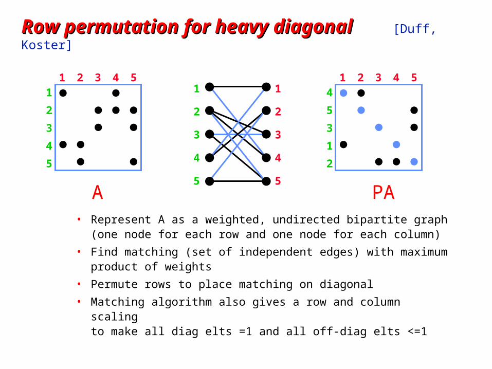
Row permutation for heavy diagonal Row permutation for heavy diagonal [Duff, Koster]
• Represent A as a weighted, undirected bipartite graph (one node for each row and one node for each column)
• Find matching (set of independent edges) with maximum product of weights
• Permute rows to place matching on diagonal
• Matching algorithm also gives a row and column scaling to make all diag elts =1 and all off-diag elts <=1
1 52 3 41
5
2
3
4
A
1
5
2
3
4
1
5
2
3
4
1 52 3 44
2
5
3
1
PA

SuperLU-dist: GE with static pivoting SuperLU-dist: GE with static pivoting [Li, Demmel]
• Target: Distributed-memory multiprocessors• Goal: No pivoting during numeric factorization
1. Permute A unsymmetrically to have large elements on the diagonal (using weighted bipartite matching)
2. Scale rows and columns to equilibrate
3. Permute A symmetrically for sparsity
4. Factor A = LU with no pivoting, fixing up small pivots:
if |aii| < ε · ||A|| then replace aii by ε1/2 · ||A||
5. Solve for x using the triangular factors: Ly = b, Ux = y
6. Improve solution by iterative refinement
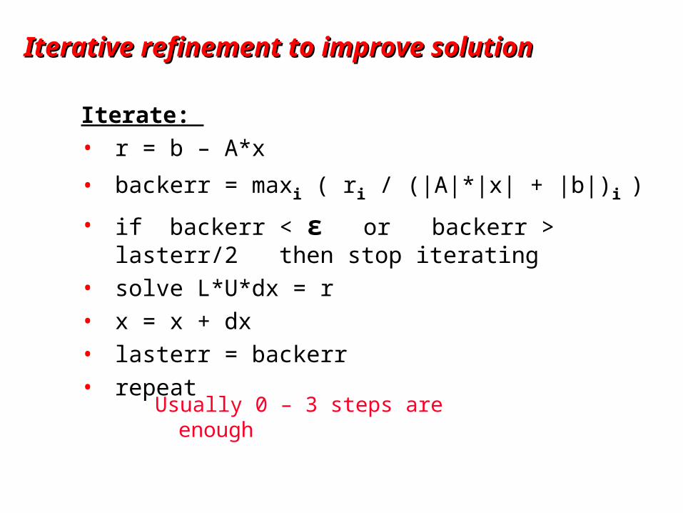
Iterative refinement to improve solutionIterative refinement to improve solution
Iterate:
• r = b – A*x
• backerr = maxi ( ri / (|A|*|x| + |b|)i )
• if backerr < ε or backerr > lasterr/2 then stop iterating
• solve L*U*dx = r
• x = x + dx
• lasterr = backerr
• repeat
Usually 0 – 3 steps are enough
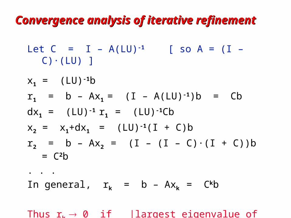
Convergence analysis of iterative refinementConvergence analysis of iterative refinement
Let C = I – A(LU)-1 [ so A = (I – C)·(LU) ]
x1 = (LU)-1b
r1 = b – Ax1 = (I – A(LU)-1)b = Cb
dx1 = (LU)-1 r1 = (LU)-1Cb
x2 = x1+dx1 = (LU)-1(I + C)b
r2 = b – Ax2 = (I – (I – C)·(I + C))b = C2b
. . .
In general, rk = b – Axk = Ckb
Thus rk 0 if |largest eigenvalue of C| < 1.
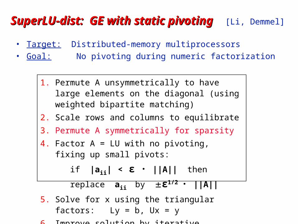
SuperLU-dist: GE with static pivoting SuperLU-dist: GE with static pivoting [Li, Demmel]
• Target: Distributed-memory multiprocessors• Goal: No pivoting during numeric factorization
1. Permute A unsymmetrically to have large elements on the diagonal (using weighted bipartite matching)
2. Scale rows and columns to equilibrate
3. Permute A symmetrically for sparsity
4. Factor A = LU with no pivoting, fixing up small pivots:
if |aii| < ε · ||A|| then replace aii by ε1/2 · ||A||
5. Solve for x using the triangular factors: Ly = b, Ux = y
6. Improve solution by iterative refinement
Directed graphDirected graph
• A is square, unsymmetric, nonzero diagonal
• Edges from rows to columns
• Symmetric permutations PAPT
1 2
3
4 7
6
5
A G(A)
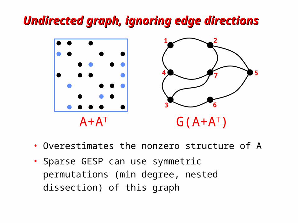
Undirected graph, ignoring edge directionsUndirected graph, ignoring edge directions
• Overestimates the nonzero structure of A
• Sparse GESP can use symmetric permutations
(min degree, nested dissection) of this graph
1 2
3
4 7
6
5
A+AT G(A+AT)
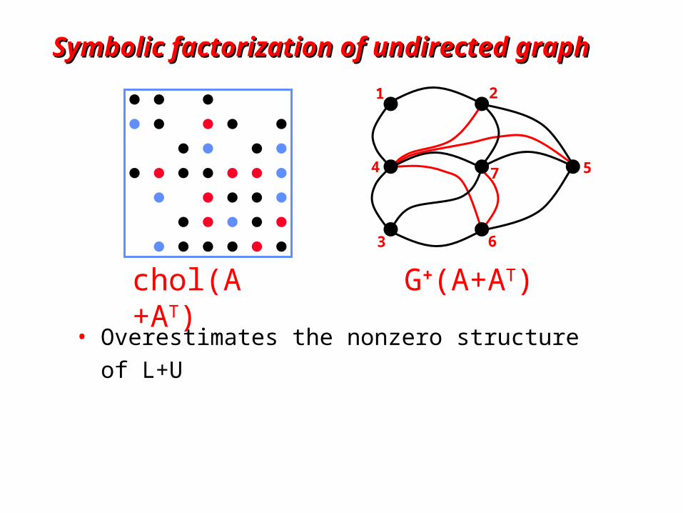
Symbolic factorization of undirected graphSymbolic factorization of undirected graph
• Overestimates the nonzero structure of L+U
chol(A +AT) G+(A+AT)
1 2
3
4 7
6
5

+
Symbolic factorization of directed graphSymbolic factorization of directed graph
• Add fill edge a -> b if there is a path from a to b
through lower-numbered vertices.
• Sparser than G+(A+AT) in general.
• But what’s a good ordering for G+(A)?
1 2
3
4 7
6
5
A G (A) L+U

Question: Preordering for GESPQuestion: Preordering for GESP
• Use directed graph model, less well understood than symmetric factorization
• Symmetric: bottom-up, top-down, hybrids• Nonsymmetric: mostly bottom-up
• Symmetric: best ordering is NP-complete, but approximation theory is based on graph partitioning (separators)
• Nonsymmetric: no approximation theory is known; partitioning is not the whole story
• Good approximations and efficient algorithms both remain to be discovered
Remarks on nonsymmetric GERemarks on nonsymmetric GE
• Multifrontal tends to be faster but use more memory
• Unsymmetric-pattern multifrontal• Lots more complicated, not simple elimination tree
• Sequential and SMP versions in UMFpack and WSMP (see web links)
• Distributed-memory unsymmetric-pattern multifrontal is a research topic
• Combinatorial preliminaries are important: ordering, etree, symbolic factorization, matching, scheduling• not well understood in many ways
• also, mostly not done in parallel
• Not mentioned: symmetric indefinite problems
• Direct-methods technology is also used in preconditioners for iterative methods
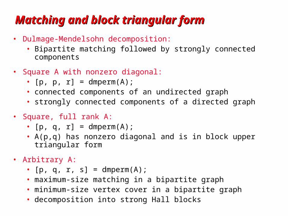
Matching and block triangular formMatching and block triangular form
• Dulmage-Mendelsohn decomposition:• Bipartite matching followed by strongly connected components
• Square A with nonzero diagonal:• [p, p, r] = dmperm(A);• connected components of an undirected graph• strongly connected components of a directed graph
• Square, full rank A:• [p, q, r] = dmperm(A);• A(p,q) has nonzero diagonal and is in block upper triangular form
• Arbitrary A:• [p, q, r, s] = dmperm(A);• maximum-size matching in a bipartite graph• minimum-size vertex cover in a bipartite graph• decomposition into strong Hall blocks
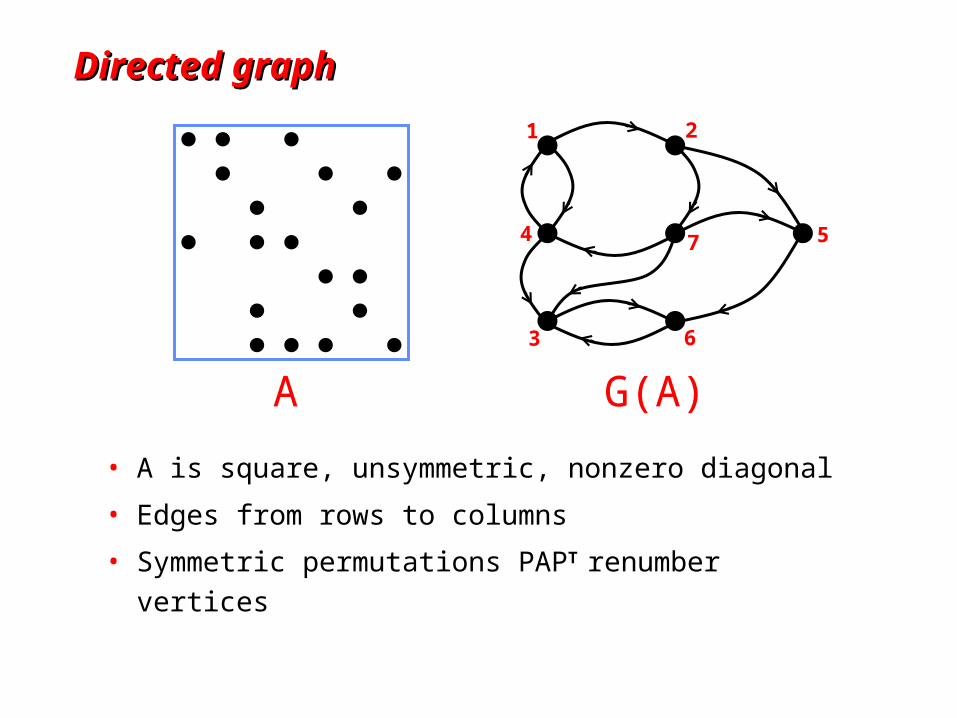
Directed graphDirected graph
• A is square, unsymmetric, nonzero diagonal
• Edges from rows to columns
• Symmetric permutations PAPT renumber vertices
1 2
3
4 7
6
5
A G(A)
1 52 4 7 3 61
5
2
4
7
3
6
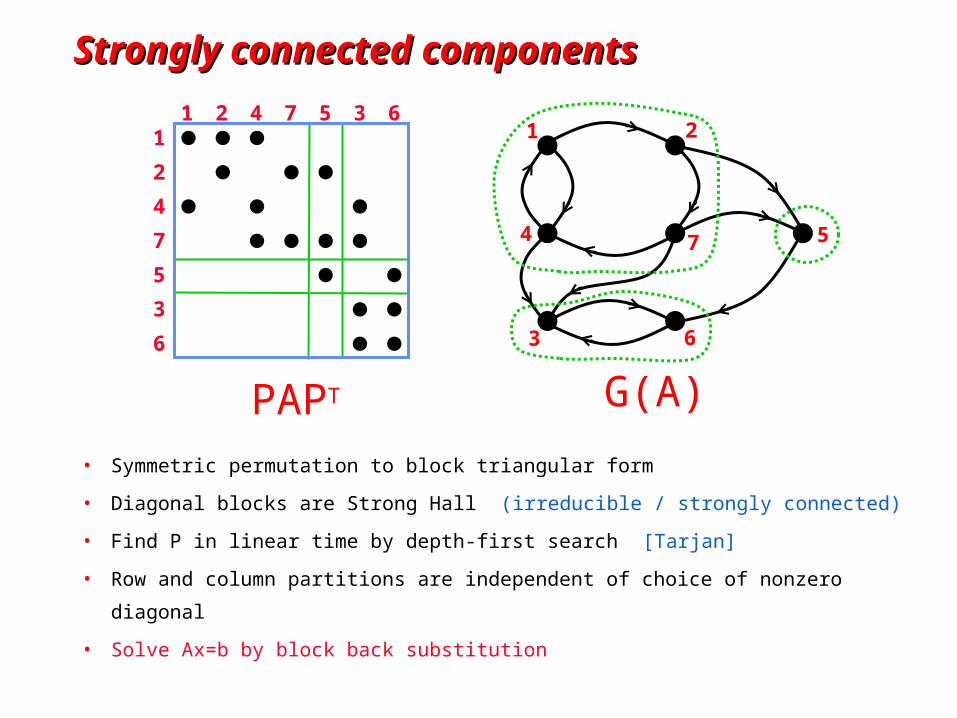
Strongly connected componentsStrongly connected components
• Symmetric permutation to block triangular form
• Diagonal blocks are Strong Hall (irreducible / strongly connected)
• Find P in linear time by depth-first search [Tarjan]
• Row and column partitions are independent of choice of nonzero diagonal
• Solve Ax=b by block back substitution
1 2
3
4 7
6
5
PAPT G(A)
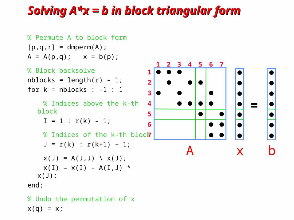
Solving A*x = b in block triangular formSolving A*x = b in block triangular form
% Permute A to block form
[p,q,r] = dmperm(A);
A = A(p,q); x = b(p);
% Block backsolve
nblocks = length(r) – 1;
for k = nblocks : –1 : 1
% Indices above the k-th block
I = 1 : r(k) – 1;
% Indices of the k-th block
J = r(k) : r(k+1) – 1;
x(J) = A(J,J) \ x(J);
x(I) = x(I) – A(I,J) * x(J);
end;
% Undo the permutation of x
x(q) = x;
1 52 3 4 6 71
5
2
3
4
6
7
=
A x b
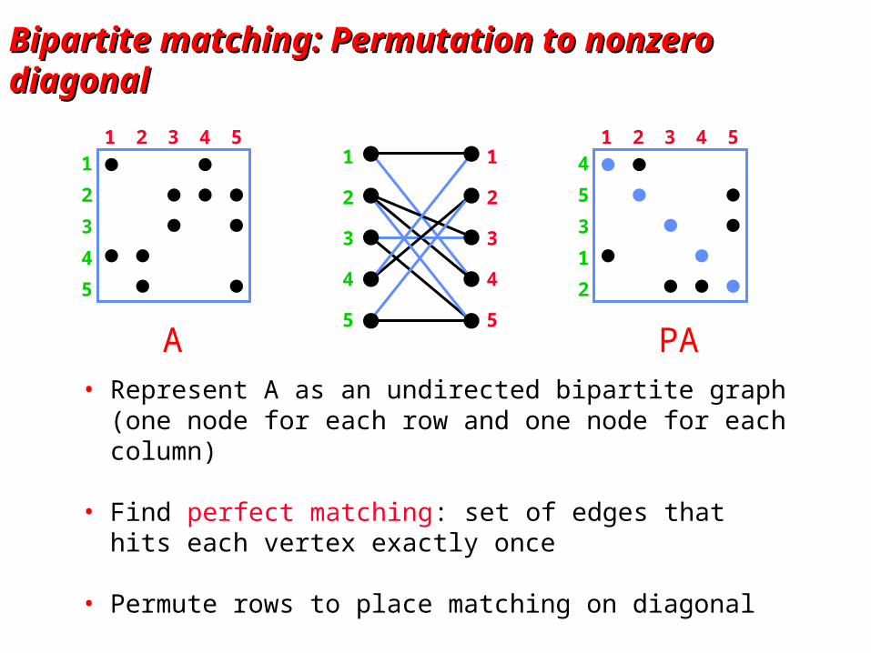
Bipartite matching: Permutation to nonzero diagonalBipartite matching: Permutation to nonzero diagonal
• Represent A as an undirected bipartite graph (one node for each row and one node for each column)
• Find perfect matching: set of edges that hits each vertex exactly once
• Permute rows to place matching on diagonal
1 52 3 41
5
2
3
4
A
1
5
2
3
4
1
5
2
3
4
1 52 3 44
2
5
3
1
PA
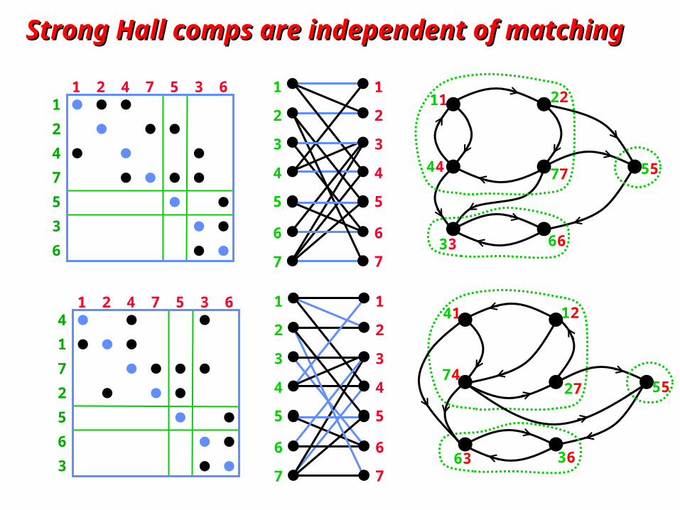
Strong Hall comps are independent of matchingStrong Hall comps are independent of matching
1 52 4 7 3 61
5
2
4
7
3
6
1 52 4 7 3 64
5
1
7
2
6
3
1
5
2
3
4
1
5
2
3
4
7
6
7
6
1
5
2
3
4
1
5
2
3
4
7
6
7
6
11 22
33
44 77
66
55
41 12
63
7427
36
55
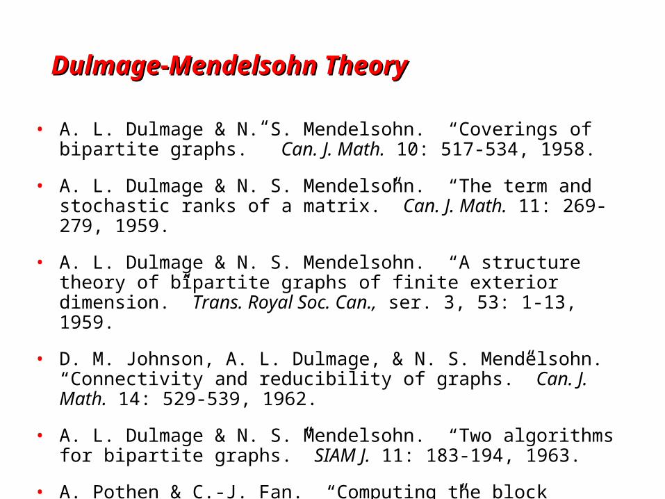
Dulmage-Mendelsohn TheoryDulmage-Mendelsohn Theory
• A. L. Dulmage & N. S. Mendelsohn. “Coverings of bipartite graphs.” Can. J. Math. 10: 517-534, 1958.
• A. L. Dulmage & N. S. Mendelsohn. “The term and stochastic ranks of a matrix.” Can. J. Math. 11: 269-279, 1959.
• A. L. Dulmage & N. S. Mendelsohn. “A structure theory of bipartite graphs of finite exterior dimension.” Trans. Royal Soc. Can., ser. 3, 53: 1-13, 1959.
• D. M. Johnson, A. L. Dulmage, & N. S. Mendelsohn. “Connectivity and reducibility of graphs.” Can. J. Math. 14: 529-539, 1962.
• A. L. Dulmage & N. S. Mendelsohn. “Two algorithms for bipartite graphs.” SIAM J. 11: 183-194, 1963.
• A. Pothen & C.-J. Fan. “Computing the block triangular form of a sparse matrix.” ACM Trans. Math. Software 16: 303-324, 1990.
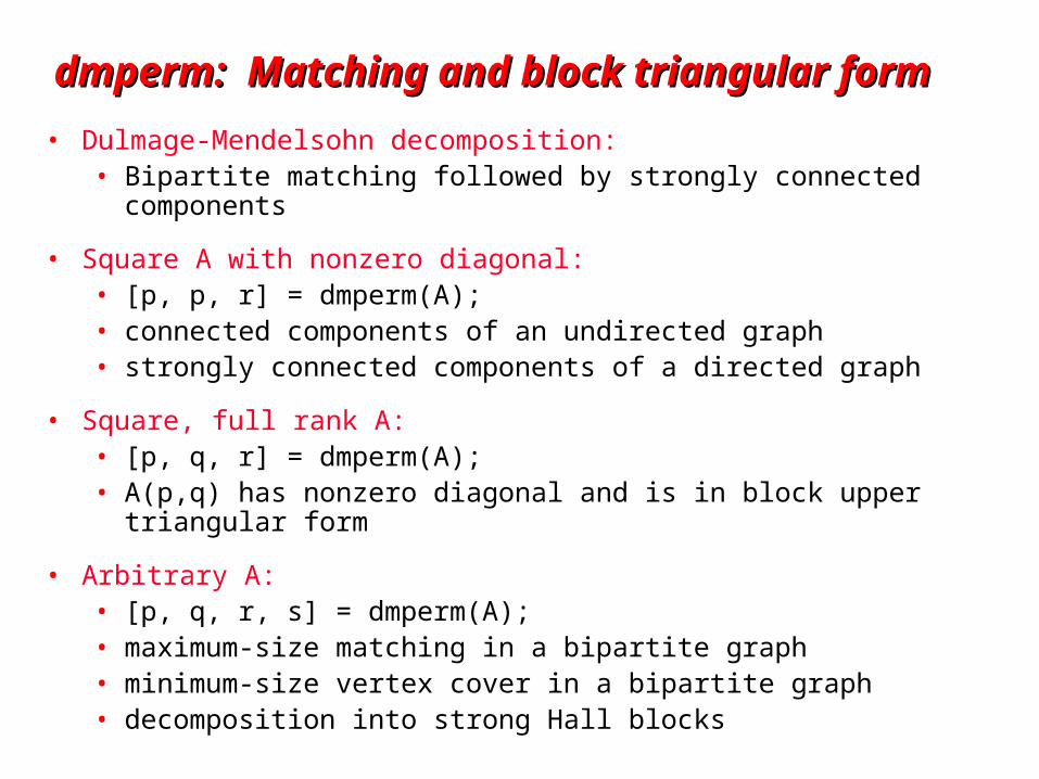
dmperm: Matching and block triangular formdmperm: Matching and block triangular form
• Dulmage-Mendelsohn decomposition:• Bipartite matching followed by strongly connected components
• Square A with nonzero diagonal:• [p, p, r] = dmperm(A);• connected components of an undirected graph• strongly connected components of a directed graph
• Square, full rank A:• [p, q, r] = dmperm(A);• A(p,q) has nonzero diagonal and is in block upper triangular form
• Arbitrary A:• [p, q, r, s] = dmperm(A);• maximum-size matching in a bipartite graph• minimum-size vertex cover in a bipartite graph• decomposition into strong Hall blocks
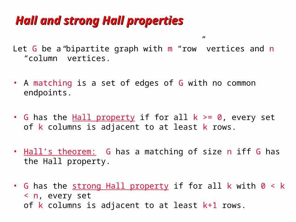
Hall and strong Hall propertiesHall and strong Hall properties
Let G be a bipartite graph with m “row” vertices and n “column” vertices.
• A matching is a set of edges of G with no common endpoints.
• G has the Hall property if for all k >= 0, every set of k columns is adjacent to at least k rows.
• Hall’s theorem: G has a matching of size n iff G has the Hall property.
• G has the strong Hall property if for all k with 0 < k < n, every set of k columns is adjacent to at least k+1 rows.
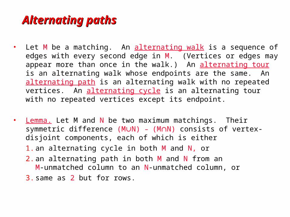
Alternating pathsAlternating paths
• Let M be a matching. An alternating walk is a sequence of edges with every second edge in M. (Vertices or edges may appear more than once in the walk.) An alternating tour is an alternating walk whose endpoints are the same. An alternating path is an alternating walk with no repeated vertices. An alternating cycle is an alternating tour with no repeated vertices except its endpoint.
• Lemma. Let M and N be two maximum matchings. Their symmetric difference (MN) – (MN) consists of vertex-disjoint components, each of which is either
1. an alternating cycle in both M and N, or
2. an alternating path in both M and N from an M-unmatched column to an N-unmatched column, or
3. same as 2 but for rows.
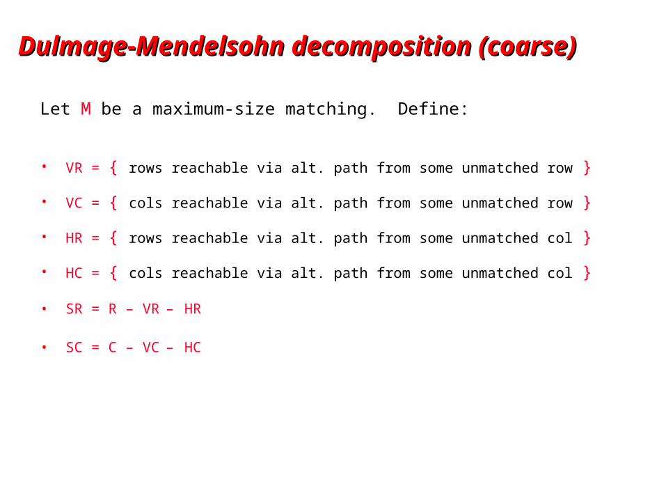
Dulmage-Mendelsohn decomposition (coarse)Dulmage-Mendelsohn decomposition (coarse)
Let M be a maximum-size matching. Define:
• VR = { rows reachable via alt. path from some unmatched row }
• VC = { cols reachable via alt. path from some unmatched row }
• HR = { rows reachable via alt. path from some unmatched col }
• HC = { cols reachable via alt. path from some unmatched col }
• SR = R – VR – HR
• SC = C – VC – HC
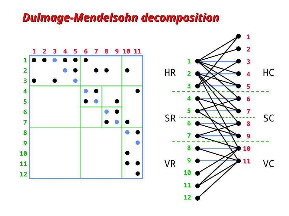
Dulmage-Mendelsohn decompositionDulmage-Mendelsohn decomposition
1
5
2
3
4
6
7
8
12
9
10
11
1 52 3 4 6 7 8 9 10 11
1
2
5
3
4
7
6
10
8
9
12
11
1
2
3
5
4
7
6
9
8
11
10
HR
SR
VR
HC
SC
VC
Dulmage-Mendelsohn theoryDulmage-Mendelsohn theory
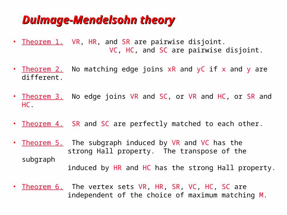
• Theorem 1. VR, HR, and SR are pairwise disjoint. VC, HC, and SC are pairwise disjoint.
• Theorem 2. No matching edge joins xR and yC if x and y are different.
• Theorem 3. No edge joins VR and SC, or VR and HC, or SR and HC.
• Theorem 4. SR and SC are perfectly matched to each other.
• Theorem 5. The subgraph induced by VR and VC has the strong Hall property. The transpose of the subgraph induced by HR and HC has the strong Hall property.
• Theorem 6. The vertex sets VR, HR, SR, VC, HC, SC are independent of the choice of maximum matching M.
Dulmage-Mendelsohn decomposition (fine)Dulmage-Mendelsohn decomposition (fine)
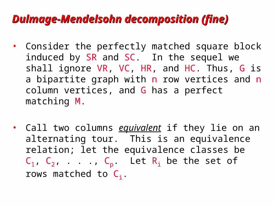
• Consider the perfectly matched square block induced by SR and SC. In the sequel we shall ignore VR, VC, HR, and HC. Thus, G is a bipartite graph with n row vertices and n column vertices, and G has a perfect matching M.
• Call two columns equivalent if they lie on an alternating tour. This is an equivalence relation; let the equivalence classes be C1, C2, . . ., Cp. Let Ri be the set of rows
matched to Ci.
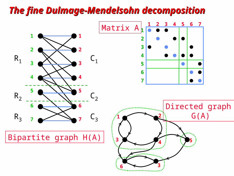
The fine Dulmage-Mendelsohn decompositionThe fine Dulmage-Mendelsohn decomposition1 52 3 4 6 7
1
5
2
3
4
6
7
1 2
6
3 4
3
5
1
5
2
3
4
1
5
2
3
4
7
6
7
6
C1R1
R2
R3
C2
C3
Matrix A
Bipartite graph H(A)
Directed graph G(A)
Dulmage-Mendelsohn theoryDulmage-Mendelsohn theory
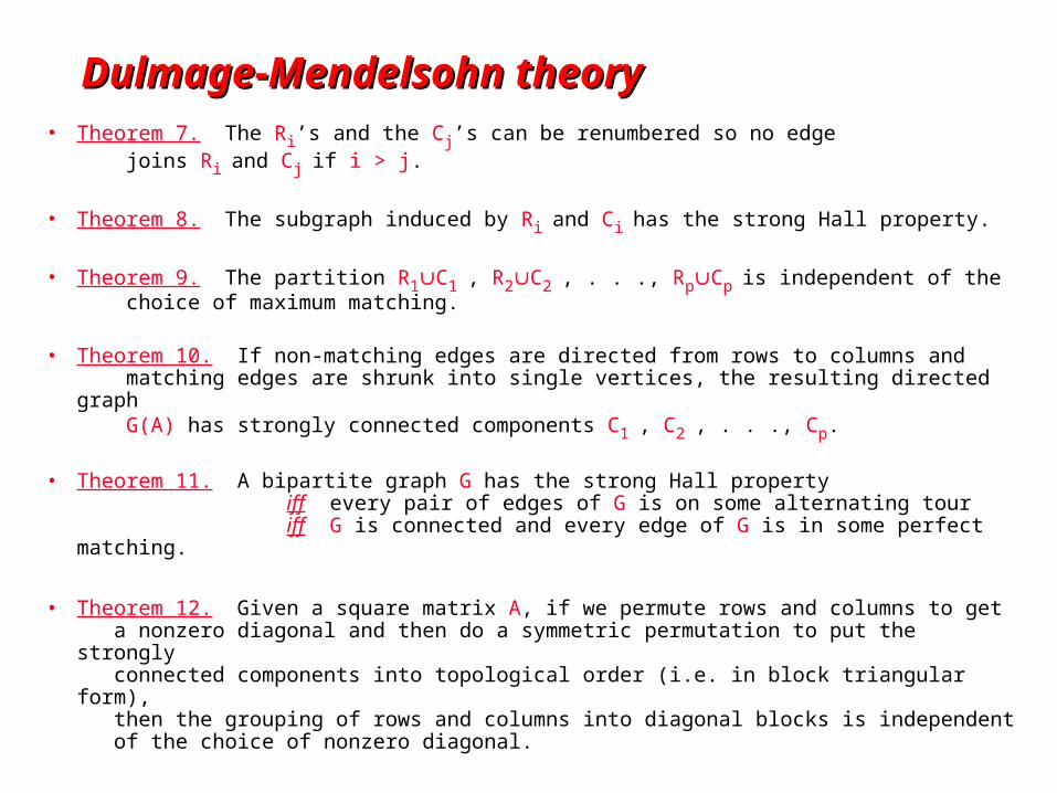
• Theorem 7. The Ri’s and the Cj’s can be renumbered so no edge joins Ri and Cj if i > j.
• Theorem 8. The subgraph induced by Ri and Ci has the strong Hall property.
• Theorem 9. The partition R1C1 , R2C2 , . . ., RpCp is independent of the choice of maximum matching.
• Theorem 10. If non-matching edges are directed from rows to columns and matching edges are shrunk into single vertices, the resulting directed graph G(A) has strongly connected components C1 , C2 , . . ., Cp.
• Theorem 11. A bipartite graph G has the strong Hall property iff every pair of edges of G is on some alternating tour iff G is connected and every edge of G is in some perfect matching.
• Theorem 12. Given a square matrix A, if we permute rows and columns to get a nonzero diagonal and then do a symmetric permutation to put the strongly connected components into topological order (i.e. in block triangular form), then the grouping of rows and columns into diagonal blocks is independent of the choice of nonzero diagonal.
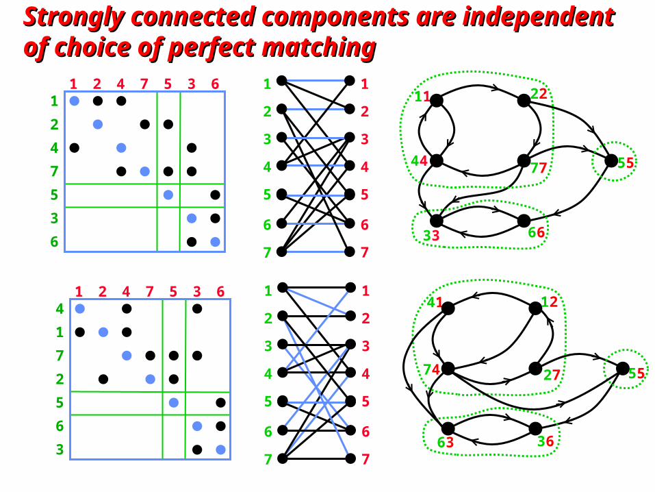
Strongly connected components are independent Strongly connected components are independent of choice of perfect matchingof choice of perfect matching
1 52 4 7 3 61
5
2
4
7
3
6
1 52 4 7 3 64
5
1
7
2
6
3
1
5
2
3
4
1
5
2
3
4
7
6
7
6
1
5
2
3
4
1
5
2
3
4
7
6
7
6
11 22
33
44 77
66
55
41 12
63
74 27
36
55
Matrix terminologyMatrix terminology
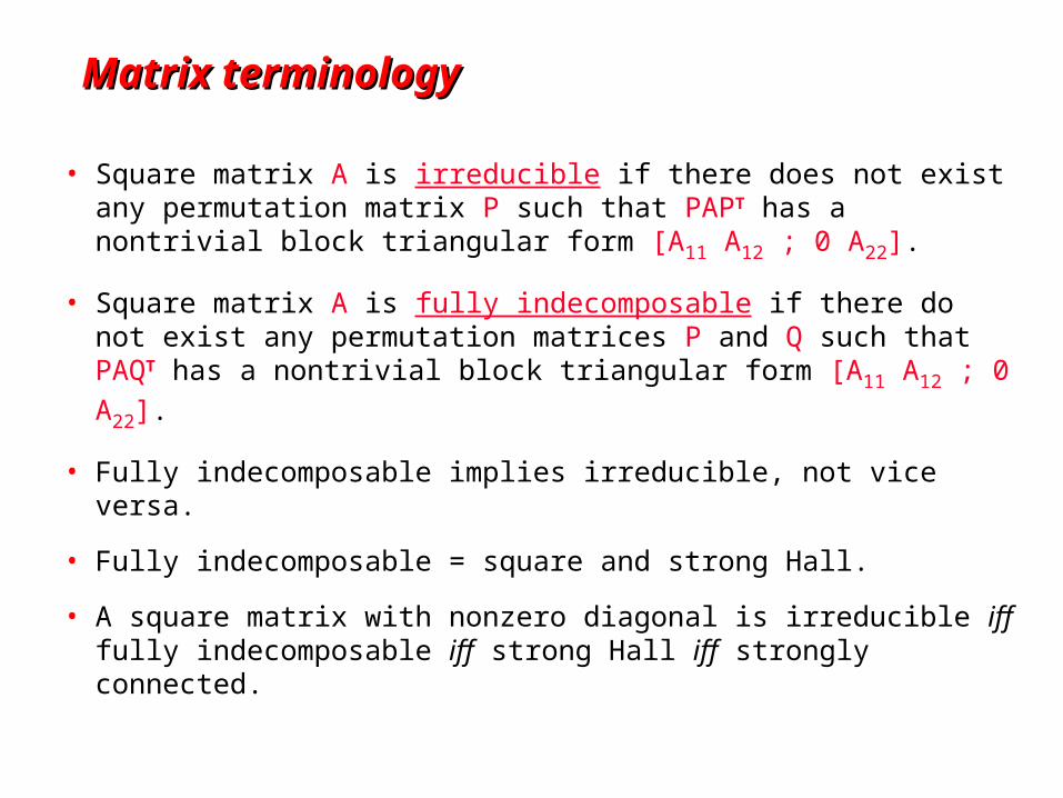
• Square matrix A is irreducible if there does not exist any permutation matrix P such that PAPT has a nontrivial block triangular form [A11 A12 ; 0 A22].
• Square matrix A is fully indecomposable if there do not exist any permutation matrices P and Q such that PAQT has a nontrivial block triangular form [A11 A12 ; 0 A22].
• Fully indecomposable implies irreducible, not vice versa.
• Fully indecomposable = square and strong Hall.
• A square matrix with nonzero diagonal is irreducible iff fully indecomposable iff strong Hall iff strongly connected.
Applications of D-M decompositionApplications of D-M decomposition
• Permutation to block triangular form for Ax=b
• Connected components of undirected graphs
• Strongly connected components of directed graphs
• Minimum-size vertex cover for bipartite graphs
• Extracting vertex separators from edge cuts for arbitrary graphs
• For strong Hall matrices, several upper bounds in nonzero structure prediction are best possible:• Column intersection graph factor is R in QR• Column intersection graph factor is tight bound on U in PA=LU• Row merge graph is tight bound on Lbar and U in PA=LU