147

Eric Ennifar (ed.), Nucleic Acid Crystallography: Methods and Protocols, Methods in Molecular Biology, vol. 1320,DOI 10.1007/978-1-4939-2763-0_10, © Springer Science+Business Media New York 2016

Chapter 10

Crystallographic Data and Model Quality

Kay Diederichs

Abstract

This article gives a consistent classification of sources of random and systematic errors in crystallographic data, and their influence on the averaged dataset obtained from a diffraction experiment. It discusses the relation between precision and accuracy and the crystallographic indicators used to estimate them, as well as topics like completeness and high-resolution cutoff. These concepts are applied in the context of pre-senting good practices for data processing with a widely used package, XDS. Recommendations are given for how to minimize the impact of several typical problems, like ice rings and shaded areas. Then, proce-dures for optimizing the processing parameters are explained. Finally, a simple graphical expression of some basic relations between data error and model error is suggested.

Key words X-ray crystallography, Accuracy, Precision, Random errors, Systematic errors, Merged data, Unmerged data, Indicators

1 Introduction

In the last decades, crystallography has been highly successful in delivering structural information about proteins, DNA, and RNA, the substrates of life on earth. The resolution of the method is good enough to discern the three dimensional structure of these macromolecules at the atomic level, which is essential to under-stand their diverse properties, functions and interactions. However, although it is easy to calculate the diffraction pattern for a given structure, the reverse task of deriving a molecular structure from just a single set of unique diffracted intensities is difficult, as the mathematical operation governing the former direction cannot be inverted in a unique way. To be solved experimentally, this “inverse problem,” or more specifically “phase problem,” requires more than just a single set of unique diffraction data. High quality of the data is a requirement for the experimental solution of the problem, but also for the refinement of the macromolecular struc-ture, as discussed in Subheading 4.

vincent.olieric@psi.ch

148

The correct biological interpretation requires the best possible model of the macromolecule. To obtain the best model, every step of the structure determination procedure has to be performed in a close-to-optimal way. This means that the purification of the mac-romolecule, its crystallization, crystal handling, measurement of diffraction data, processing of the resulting datasets, and down-stream steps such as structure solution, refinement, and validation each constitute scientific tasks that deserve specific attention, and have been undergoing continuous enhancements throughout the history of macromolecular crystallography.

Two kinds of numerical data are the result of a crystallographic experiment and usually deposited as such in the Protein Data Bank: the diffraction intensities as a reduced representation of the diffrac-tion experiment, and the atomic coordinates resulting from the visual inspection and interpretation of electron density maps, and subsequent refinement. A third kind of numerical data, the raw data (frames) obtained in the diffraction experiment, have so far not been usually deposited in long-term archives, mainly due to (disk) space concerns. This is unfortunate since archiving of raw data would enable reprocessing of incorrectly processed data as well as enabling and taking advantage of future improvements in methodology, like extracting the diffuse scattering information.

The discussion focuses on data that correspond to a single atomic model. This rules out all the complications that arise from merging of non-isomorphous datasets, where each individual data-set corresponds to a different model—in this situation, a merged dataset would represent something like an average model, which violates the physicochemical requirements, and may not be bio-logically meaningful.

This chapter first presents the principles and concepts that need to be understood in the context of the rather broadly used term “data quality”; similar presentations may be found for exam-ple in refs. [1–3]. Second, the application of these principles to data processing with the XDS program package [4, 5], which the author is most familiar with, is explained. Third, data and atomic model are related in a graphical way, which allows some important and nontrivial conclusions to be drawn about how the former influence the latter.

2 Errors and Crystallographic Indicators

The goal of a crystallographic experiment is to obtain accurate intensities I(hkl) for as many Bragg reflections hkl as possible. I discuss two kinds of errors, random and systematic error, which exist in any experiment. A major difference between them is that the relative error arising from the random component decreases with increasing intensity, whereas the relative error in intensity

Kay Diederichs

vincent.olieric@psi.ch

149

from the systematic component is (at least on average) constant, often in the range between 1 and 10 %. A more specific descrip-tion for systematic error would thus be “fractional error,” but this name is not in common use. Nonlinear errors also exist, but play a minor role.

A well-designed crystallographic experiment has to strike an appropriate compromise between the two kinds of error. For example, a reduction of random error (see below) can be obtained by longer or stronger exposure of the crystal, but this will inevita-bly increase the systematic error from radiation damage to the crystal. Ideally, the sum of both errors should be minimal, and programs, e.g., “BEST” [6], exist that suggest a compromise, in the form of a proposed “strategy” for the experiment. Fortunately, the gradient of the sum of both errors is close to zero at and near the optimal strategy, which means that small deviations from the optimal strategy do not substantially decrease data quality.

The discussion of errors has to take the distinction between precision and accuracy into account. The term “precision” refers to the reproducibility of an experiment, and to the internal consis-tency or relative deviation of the values obtained. For example, if the number e = 2.718… should be determined in an experiment, and two measurements would yield the values 3.217 and 3.219, then these measurements are considered precise, because they agree well with each other—their relative deviation is small. However, they are not close to the true value—the error (or inac-curacy) in their measurement amounts to about 0.5.

The term “accuracy,” on the other hand, refers to the devia-tion of measured values from the true values. In this example, if two measurements would yield the values 2.6 and 2.8, then the results from this experiment are more accurate than that from the previously mentioned experiment, although they are not as precise.

Optimizing an experiment for precision alone therefore does not ensure accuracy; rather, equating accuracy with precision also requires the absence of any kind of error that has not been taken into account in the precision estimate. To estimate accuracy, we thus need to quantify both the precision of the data, and the unde-tected error (which usually requires some knowledge about the true value obtained by other means). If both can be quantified, we can estimate the accuracy as the absolute or relative error of a measurement.

The crystallographic experiment measures the number of photons contributing to each detector pixel. These photons arise from Bragg reflections, but also from background scatter. The number of photons in each pixel is subject to random fluctuations. These are due to the quantum nature of photons; there exists a certain probability of emission of a given photon by the crystal into a given

2.1 Random Error

Data and Model Quality

vincent.olieric@psi.ch

150

pixel in a unit of time, and each photon’s emission into that pixel is independent from that of other photons. As a result, photon counts are governed by Poisson (counting) statistics, which math-ematically means that the variance of the photon number is equal to the photon number itself. Furthermore, a CCD detector may contribute a random component (“read-out noise”) to the total photon count (pixel detectors are almost noise-free), which is also due to quantum fluctuations in the detector hardware and may be considered as additional background.

Data processing software essentially adds the counts of the pix-els belonging to each reflection, and subtracts an estimate of the background in each pixel, to give I(hkl), the intensity of the Bragg reflection. The variance of I(hkl) may be calculated, using the rules of error propagation, from the known variances of each contribu-tion to I(hkl); its square root will be called σ0(hkl) in the following. For strong reflections, where the background is negligible, this procedure gives a precision, expressed as relative random error in I(hkl), of σ0(hkl)/I(hkl) ~ 1/√I(hkl).

The relative amount of the random error may be reduced by repeating the experiment, and averaging the results of the indi-vidual experiments. As the laws of error propagation show, the pre-cision of the estimate of the averaged intensity is improved by a factor of √n over that of an individual measurement, if n is the number of repeated experiments with independent errors. Thus, the precision of the averaged (also called “merged”) data may be high even if the precision of each individual observation is low.

The square root function appears both in the relative error of a photon count arising from Poisson statistics, and in the improve-ment of precision from averaging of multiple measurements. It is important to realize that the mathematical reasons for the occur-rence of the square root differ. Nevertheless, the fact that the square root occurs in both situations means that the relative error is in principle the same whether a reflection is measured ten times and averaged, or measured just once, but with ten times stronger exposure or ten times as long.

A high number (multiplicity, sometimes called redundancy) of observations of each unique reflection, together with low exposure of each observation, is therefore equivalent in terms of the preci-sion of the merged data, to an experiment in which each unique reflection is just measured once, but exposed proportionally stron-ger. Thus, if only random error is considered, there would be no reason to perform experiments with high multiplicity.

The term “systematic error” summarizes all types of error that are not purely random in nature, and these are due to macroscopic physical or technical properties of the experimental setup, the crys-tal, and the processing of its data. For instance, systematic errors may arise from imperfect spot shapes (split crystal), radiation

2.2 Systematic Error

Kay Diederichs

vincent.olieric@psi.ch

151

damage, absorption differences due to crystal shape and mounting, shutter synchronization problems, imperfect detector calibration and inhomogeneity of detector sensitivity, shadowed parts of the detector, nonlinear or overloaded detector, vibrations for example due to the cryo stream or fluctuations of the primary X-ray beam, imperfect or inaccurate assumptions about geometric parameters and computational models applied in the data processing step, and to other problems that may be significant for a given experiment.

Systematic error may appear to be random if its cause is unknown or cannot be fully described or modelled, but contrary to random counting error, the change of a reflection’s intensity is usually (at least on average) proportional to the intensity itself—thus the term “fractional error.” For example, a fluctuation in beam intensity changes all intensity values by the same percentage; absorption in the crystal or loop changes intensities in proportion to their original value; and using, during data processing, a mosaic-ity value that is too low, or a summation (integration) area that is too small, will chop off a certain fraction of the intensity.

Contrary to random error, the relative error of a single obser-vation is not decreased by higher flux or longer exposure. However, many kinds of systematic errors in a crystallographic experiment at least partially cancel out if multiple measurements are averaged. This is the case if the experiment samples the possible values of the error term multiple times, in an even (or at least random) and unbiased way. Examples are beam instability, shutter problems, and most aspects of detector non-ideality, except those that result in nonlinear response (e.g., overload). Their influence on the final averaged data is decreased by averaging of n independent observa-tions, and indeed the reduction of error then follows the same √n rule as applies to random error.

These kinds of systematic error may thus be considered as benign: their influence on the merged data may be mitigated by distributing the total experimental time and dose over many obser-vations, or by collecting multiple datasets [7]. It is therefore sys-tematic error, not random error, that mandates the collection of data over more than the absolute minimum of rotation range required for obtaining complete data. However, it is important to realize that after a full turn of the spindle, all those systematic errors that depend on the geometry of the experiment will be exactly repeated. It is thus highly advisable to change the crystal setting on the goniostat after at most 360°.

If all or most observations of a unique reflection are systemati-cally affected in the same or a similar way, their systematic errors are not independent, and averaging may not necessarily decrease the systematic difference between true and estimated intensity (the accuracy). Known or well understood effects may often be mod-elled by analytical or empirical formulas. If a model for the specific error type is available and appropriate, the systematic difference is

Data and Model Quality

vincent.olieric@psi.ch

152

accounted for, and any remaining difference between intensities may become a useful signal. In this way, a systematic effect may become a part of an extended description of the experiment, and does no longer contribute to the experimental error.

An example for this is absorption by the crystal and its environ-ment (loop, mother liquor)—if it can be properly modelled, its influence is compensated. However, in low-symmetry space groups, all symmetry-related reflections may systematically be weakened or strengthened in the same way. Since only those sys-tematic errors that lead to systematic differences can be corrected, no information about the proper absorption correction is available in this case. Therefore, at least one additional dataset should be measured in a different orientation of the crystal. The systematic absorption difference between the two resulting datasets may then be detected and corrected in software. It should be noted that even if absorption is not corrected in the data processing stage, it can be approximately compensated by an overall anisotropic overall dis-placement parameter in the refinement stage. This parameter then should not be interpreted as its name suggests, but rather as a com-pensation factor for an experimental property.

Importantly, for strong reflections (low resolution), systematic error is usually higher than random error; the converse is true for weak reflections (high resolution), where the signal-to-noise ratio is usually dominated by the random error term. However, radia-tion damage, the most devastating kind of systematic error, is an exception to this rule. Radiation damage, which changes (and ulti-mately destroys) the structure of the macromolecule during the measurement, induces a systematic error that is not mitigated by averaging of multiple observations, because it results in intensity measurements that do not scatter around a true value, but rather, with increasing dose, deviate further and further from the true value—the intensity at the beginning of the experiment.

The detrimental influence of radiation damage has to be avoided to a degree that depends on the kind of experiment, and its desired goal. In recent years, there has been some progress in describing the relation between dose and its footprint on the mac-romolecule [8, 9]. Furthermore, the influence of radiation damage may be partially compensated by zero-dose extrapolation, a com-putational technique [10]. However, it should be noted that the relative change of intensities by radiation damage is biggest at high resolution, where the signal may be so weak (i.e., the individual measurements so imprecise) that zero-dose extrapolation becomes inaccurate.

The error estimates σ0(hkl) obtained during integration of observa-tions, being only based on counting statistics, are lower than the actual differences between intensities of symmetry-related observa-tions, because the latter include the differences due to systematic

2.3 An Indicator for the Systematic Error

Kay Diederichs

vincent.olieric@psi.ch

153

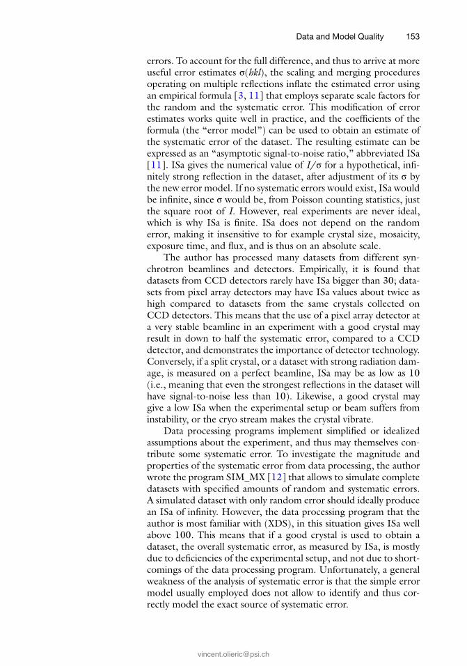
errors. To account for the full difference, and thus to arrive at more useful error estimates σ(hkl), the scaling and merging procedures operating on multiple reflections inflate the estimated error using an empirical formula [3, 11] that employs separate scale factors for the random and the systematic error. This modification of error estimates works quite well in practice, and the coefficients of the formula (the “error model”) can be used to obtain an estimate of the systematic error of the dataset. The resulting estimate can be expressed as an “asymptotic signal-to-noise ratio,” abbreviated ISa [11]. ISa gives the numerical value of I/σ for a hypothetical, infi-nitely strong reflection in the dataset, after adjustment of its σ by the new error model. If no systematic errors would exist, ISa would be infinite, since σ would be, from Poisson counting statistics, just the square root of I. However, real experiments are never ideal, which is why ISa is finite. ISa does not depend on the random error, making it insensitive to for example crystal size, mosaicity, exposure time, and flux, and is thus on an absolute scale.

The author has processed many datasets from different syn-chrotron beamlines and detectors. Empirically, it is found that datasets from CCD detectors rarely have ISa bigger than 30; data-sets from pixel array detectors may have ISa values about twice as high compared to datasets from the same crystals collected on CCD detectors. This means that the use of a pixel array detector at a very stable beamline in an experiment with a good crystal may result in down to half the systematic error, compared to a CCD detector, and demonstrates the importance of detector technology. Conversely, if a split crystal, or a dataset with strong radiation dam-age, is measured on a perfect beamline, ISa may be as low as 10 (i.e., meaning that even the strongest reflections in the dataset will have signal-to-noise less than 10). Likewise, a good crystal may give a low ISa when the experimental setup or beam suffers from instability, or the cryo stream makes the crystal vibrate.

Data processing programs implement simplified or idealized assumptions about the experiment, and thus may themselves con-tribute some systematic error. To investigate the magnitude and properties of the systematic error from data processing, the author wrote the program SIM_MX [12] that allows to simulate complete datasets with specified amounts of random and systematic errors. A simulated dataset with only random error should ideally produce an ISa of infinity. However, the data processing program that the author is most familiar with (XDS), in this situation gives ISa well above 100. This means that if a good crystal is used to obtain a dataset, the overall systematic error, as measured by ISa, is mostly due to deficiencies of the experimental setup, and not due to short-comings of the data processing program. Unfortunately, a general weakness of the analysis of systematic error is that the simple error model usually employed does not allow to identify and thus cor-rectly model the exact source of systematic error.

Data and Model Quality

vincent.olieric@psi.ch

154

Conceptually, it is almost always impossible to accurately measure the systematic error, since the true intensities are unknown and not measurable. Obviously, ISa underestimates the overall sys-tematic error, as only those systematic errors that lead to systematic differences enter its calculation. In my research group, we usually find that upon scaling two or more datasets together, the new error model for each dataset, which is calculated by the scaling program (XSCALE), almost always leads to a reduction of its ISa. This is due to the fact that only by comparing datasets can some system-atic errors be detected.

For isomorphous datasets (e.g., same crystal but different ori-entation) which are >90 % complete, have average multiplicity of 3 and more, and have higher symmetry than triclinic, we find that the reduction of ISa is usually less than 10 %. Therefore, the under-estimation of the systematic error by ISa is usually minor.

If non-isomorphous crystals are scaled and merged and the error model is recalculated, the newly determined ISa values have to account for the systematic differences arising from differences in unit-cell parameters and crystal contents, and may then be much reduced.

In crystallography, indicators to describe aggregated properties of the data are necessary because the number of reflections is so large that it is prohibitive to inspect individual reflections. The availabil-ity of multiple observations (called “multiplicity” or “redundancy”) allows their precision to be measured.

Historically, Rsym was proposed by Arndt [13] for analysis of data from the first electronic area detectors. At the time, his inter-est was to create an indicator for how reproducibly the data are measured with these devices. This lead him to use a formula simi-lar to the “R-factor,” which has been in use since before the mid-dle of last century (for example in [14]), and compares the experimental amplitudes with those derived from a model. His formula

R

I hkl I hkl

I hkl

i j

n

j

i j

n

j

i

isym =( ) - ( )

( )

åå

åå=

=

1

1

calculates the relative absolute deviation of intensity measurements from their mean value. Rsym has been in use since then, but renamed to Rmerge probably because the formula can also be applied when merging symmetry-equivalent observations obtained from one or more crystals. Rmerge measures the precision of the individual mea-surements (observations) of the intensities, and takes both the

2.4 Indicators for the Precision of Unmerged Data

Kay Diederichs

vincent.olieric@psi.ch

155

random and systematic error into account, in as far as the latter leads to differences in symmetry-related reflections.

It turned out that Rmerge, as originally defined, has the flaw that for low multiplicity datasets it makes the precision appear to be better than it really is (by up to a factor of √2; [15]). This can be

fixed by including a factor n

ni

i -1 in the numerator [15], and the

resulting precision indicator is called Rmeas (or Rr.i.m.; [16]). Even though it more accurately reflects the precision of the data, it has unfortunately not been fully adopted by the crystallographic com-munity; mainly, I assume, for the psychological reason that Rmeas has a higher numerical value than Rmerge.

Another measure of precision of intensities is the average I/σ ratio of the observations, ‹I/σ›obs. Rmeas and ‹I/σ›obs obey Rmeas ~ 0.8/‹I/σ›obs. This approximate relation is valid provided that the error model has been adjusted such that χ2, an indicator of the agreement between estimated and observed differences between symmetry-related observations, is near 1, and provided that ‹I/σ› is a good approximation of ‹I›/‹σ›. For a given dataset, these approximations are usually well fulfilled at high resolution. Nevertheless, the error models of different data processing pro-grams usually yield quite different estimates of the σ(hkl) and ‹I/σ›obs values [17].

A precision indicator like Rmeas or ‹I/σ›obs is only useful in com-parisons of datasets if the multiplicity of observations in the com-pared datasets is approximately the same. However, neither measure is useful for defining, for instance, a high-resolution cutoff since it does not take into account the obvious fact that multiple observations increase the precision.

The low-resolution Rmeas value of a strongly exposed crystal mainly measures detectable systematic error and may therefore be considered another indicator of systematic error. This may explain the historical popularity of the related (but less suitable) Rsym value for (broadly) characterizing the “quality” of a dataset.

With one exception [18], merged data are used in all crystallo-graphic calculations after the data processing step. Statistics refer-ring to merged data are thus much more important than those referring to unmerged data, and ignorance or misunderstanding of this fact has led to common misconceptions about for example the choice data collection strategy, the choice of dataset to refine against, the possibility of merging of datasets, and about a suitable high-resolution cutoff [19].

In 1997, Diederichs and Karplus [15] therefore introduced a specially defined R-value which takes the multiplicity of observa-tions into account, and calculates the precision of the merged data. This quantity, Rmrgd-I, measures the differences between merged

2.5 Indicators for the Precision of Merged Data

Data and Model Quality

vincent.olieric@psi.ch

156

intensities from two randomly selected subsets of the data. It is not in common use, but Rsplit,

RI I

I I

i

i

split

even odd

even odd

=-

+

å

å1

2 12

which is the same as Rmrgd-I except for a factor of 1/√2 and a sim-plified assignment of measurements to subsets, is in use by the Free Electron Laser community [20]. An equivalent quantity, Rp.i.m. (“precision indicating merging R-factor”; [16])

Rn

I hkl I hkl

I hkl

i i j

n

j

i j

n

j

i

ipim =-

( ) - ( )

( )

å å

åå

=

=

1

1 1

1

takes the √n improvement of precision directly into account, and has been shown to be useful when compared to Ranom which mea-sures the precision of the anomalous signal.

High-resolution R-values go to infinity when the signal van-ishes [19]. This is obvious from the fact that the mean intensity, in the denominator of the formula, approaches zero in this situation, whereas the numerator approaches a constant which is determined by the variance of the background. This prevents the aforemen-tioned data R-values from being useful for comparisons with model R-values at vanishing signal, where the latter approach a constant value [21]. As a consequence, data R-values are not suitable for defining a high-resolution cutoff, a little-known fact that has led to wrong conclusions for numerous datasets.

One of the oldest and more useful estimators of precision is ‹I/σ›mrgd (the subscript “mrgd“ is added here only to distinguish it from ‹I/σ›obs; the subscript is not in common use) of the averaged data, which most data processing programs print out. There exists a reciprocal relationship between ‹I/σ›mrgd and Rmrgd-I/Rsplit/Rp.i.m. similar to the relation between ‹I/σ›obs and Rmeas. Unfortunately, the value of ‹I/σ›mrgd depends on the error model, which usually varies significantly between different data processing programs [17]. Furthermore, for a given error model, ‹I/σ›mrgd rises monot-onously with higher multiplicity, even if the additional data are bad, e.g., in case of radiation damage. Nevertheless, historically a value of ‹I/σ›mrgd > 2 has been and continues to be used by many crystallographers as indicating the highest resolution shell that should be used for refinement [3, 22].

The latest, statistically justifiable and so far most useful addi-tion to the crystallographic data precision indicators is CC1/2, which is derived from mainstream statistics and measures the

Kay Diederichs

vincent.olieric@psi.ch

157

correlation coefficient between merged intensities obtained from two random subsets of the data. Its properties have been investi-gated recently [19, 23, 24]. It does not depend on estimated stan-dard deviations of intensities, and its value is not misleadingly increased by important types of systematic errors [23]. Being a correlation coefficient, its value can be assessed for significance by a t-test, and most importantly, it offers the possibility to define a high- resolution cutoff based on the question “where do the data still have significant signal.”

Furthermore, from CC1/2 we can calculate CC*, a quantity on the same scale as correlation coefficients between measured inten-sities and Fcalc

2 that are obtained from a model [19]. The latter, termed CCwork/CCfree, are defined for the “working” and the “free” set of reflections used in refinement, and should converge towards CC* in the course of model completion and correction.

Since the true intensity values are usually unknown and not mea-surable, in a strict sense it is impossible to estimate the accuracy of the merged intensity values, because undetected systematic error may be present which has to be added to the error estimate corre-sponding to the precision of the merged data.

As discussed, a few sources of systematic error remain poten-tially undetected; most notable are absorption, diffuse scattering and detector nonlinearity. Experience suggests that the undetected systematic error in the merged data may be on the order of a few percent for a good experiment; this is the relative difference between observed data and calculated intensities seen in small- molecule experiments where a complete and accurate model of the structure is available. A more quantitative, but still conserva-tive upper limit is the reciprocal of ISa: this estimate asserts that the undetected systematic error is unlikely to be higher than the detected systematic error.

It is important to realize that when adding independent errors or error estimates, error propagation tells us that we have to add their squares, and finally take the square root. To give an example: suppose we expect an undetected relative systematic error of 3 % (conservative upper limit at ISa = 33), and a detected relative sys-tematic error of 1.5 % (corresponding to ISa = 33 and fourfold multiplicity). In a low-resolution shell of a crystal, the random error in the merged data may amount to 2 %. We then have a rela-tive accuracy estimate of about 4 % (√(0.032 + 0.0152 + 0.022) = 0.039). In a resolution shell with 20 % relative random error in the merged data, we have a relative accuracy estimate of slightly more than 20 % (√(0.032 + 0.0152 + 0.202) = 0.203). Thus, in practice, the estimate of the undetected error dominates the accuracy esti-mate of the strong low-resolution data, whereas for weak high- resolution data, the accuracy estimate is determined mostly by the precision of the merged data.

2.6 Accuracy of the Merged Data

Data and Model Quality

vincent.olieric@psi.ch

158

All reflections in a dataset contribute to any place in the Fourier synthesis of the electron density. In principle, this means that the quality of the electron density map is compromised if not all reflec-tions are measured. Quantitatively, since the reflections contribute to the map in proportion to their amplitude, it is clear that the strongest reflections are most important. Strong reflections are found mainly at low resolution, where completeness fortunately is favoured by the geometry of the diffraction experiment, i.e., the low-resolution shells are usually more complete than the high- resolution shells. Then again, the strongest reflections are those that are most easily lost due to detector overload, which means that another dataset (“low resolution pass”) may be needed to fill in the missing (that is, saturated and thus inaccurate) reflections.

There exist no hard rules or studies about how incomplete data may be to be still useful. If non-crystallographic symmetry is present, averaging of the electron density maps of the copies of the molecule may be performed, which partly substitutes for missing completeness by virtue of redundancy in the unique dataset. If only a single copy of the molecule resides in the asymmetric unit, a low-resolution completeness of less than 75 % can be expected to lead to quite noticeable degradation (artifacts) of maps (for an example, see http://ucxray.berkeley.edu/~jamesh/movies/ completeness.mpeg); also, data missing systematically in a region of reciprocal space leads to more noticeable defects in the electron density than randomly missing data (http://www.ysbl.york.ac.uk/~cowtan/fourier/duck4.html). On the other hand, if the low resolution is almost complete, there is no reason to discard high- resolution shells just for lack of completeness. To the contrary: all measured reflections are valuable as they mitigate Fourier ripples, contribute to the fine details in the electron density map, and constitute use-ful restraints in refinement. The common practice of discarding high-resolution data if their completeness is not “high enough” is questionable, and has never been carefully tested.

3 How to Obtain the Best Data from XDS

The procedures for processing data with XDS have been described [4, 5] and are not repeated here. Instead, based on first hand expe-riences when processing datasets from my own group and helping others with their challenging datasets, I focus on those steps that are critical for data quality. For simplicity, we assume that a given dataset can be indexed in the correct space group.

The overarching rules for data processing, in the order of their importance, are that

(a) Sources of systematic error should be excluded if possible. (b) The impact of any remaining sources of systematic error on

the data should be minimized.

2.7 Completeness

Kay Diederichs

vincent.olieric@psi.ch

159

(c) The random error should be minimized. (d) The completeness of the data should be maximized.

Experience shows that goals (a), (b), and (c) are not conflict-ing, but can be met with the same set of processing parameters. Topic (d), however, requires a compromise. For instance, rejecting the final frames of a dataset, in order to minimize the impact of radiation damage, will reduce the completeness, or at least the multiplicity of the data. Likewise, too generous masking of shad-owed detector regions might lead to rejection of well-measured reflections.

Analysis of the information provided by XDS (see below) may lead to deeper insight about the data collection experiment itself. Designing and evaluating an experiment is a genuinely scientific approach and can and should not be left to automatic procedures.

The goal of data processing is to best parameterize the data collection experiment. If the data processing is repeated with changed parameters, the magnitude of the systematic error should be monitored, using ISa. By optimizing (maximizing) ISa, indica-tors of data precision are usually enhanced along the way, mainly because the location and shape of the reflections on the frames can be predicted more accurately. Generally, if the systematic error in the data is reduced, the noise associated with it is con-verted to signal. In case of doubt about any specific aspect of data processing, the parameter value that maximizes ISa is usually the correct one.

To discover problems associated with data processing, it is essential that in particular the files FRAME.cbf, INTEGRATE.LP, XDS_ASCII.HKL and CORRECT.LP are analyzed.

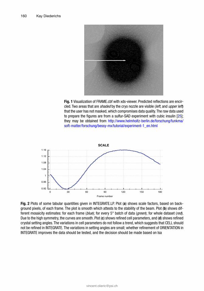
FRAME.cbf should be inspected (Fig. 1) to find out whether spot shapes are regular, or whether there is indication of splitting and multiple lattices. Irregular and split spots indicate problems in crystal growth or handling, and always compromise data quality due to higher random noise (because spots extend over more pix-els) and higher systematic error (because the reflection profiles dif-fer from the average). Furthermore, FRAME.cbf allows finding out if predicted and observed diffraction patterns match. If they do not, the space group or geometric parameters may be wrong which may either prevent data processing from giving useful data, or may lead to downstream problems in phasing and refinement. However, this is beyond the scope of this article. Finally, FRAME.cbf, which visualizes the last frame processed by INTEGRATE, should be checked for the presence of ice rings (see below).

The tables in INTEGRATE.LP should be inspected for jumps or large changes in frame-wise parameters like scale factors, mosa-icity, beam divergence, or refined parameters like unit cell param-eters, direct beam position, and distance (Fig. 2). Such changes

3.1 General Approach

Data and Model Quality

vincent.olieric@psi.ch

160

Fig. 1 Visualization of FRAME.cbf with xds-viewer. Predicted reflections are encir-cled. Two areas that are shaded by the cryo nozzle are visible (left, and upper left) that the user has not masked, which compromises data quality. The raw data used to prepare the figures are from a sulfur-SAD experiment with cubic insulin [25]; they may be obtained from http://www.helmholtz-berlin.de/forschung/funkma/soft-matter/forschung/bessy-mx/tutorial/experiment-1_en.html

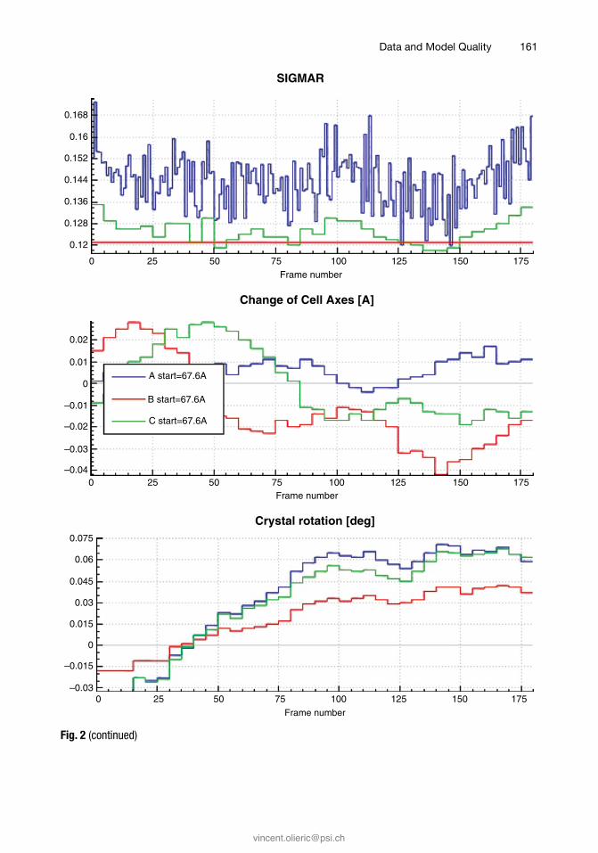
Fig. 2 Plots of some tabular quantities given in INTEGRATE.LP. Plot (a) shows scale factors, based on back-ground pixels, of each frame. The plot is smooth which attests to the stability of the beam. Plot (b) shows dif-ferent mosaicity estimates: for each frame (blue); for every 5° batch of data (green); for whole dataset (red). Due to the high symmetry, the curves are smooth. Plot (c) shows refined cell parameters, and (d) shows refined crystal setting angles. The variations in cell parameters do not follow a trend, which suggests that CELL should not be refined in INTEGRATE. The variations in setting angles are small; whether refinement of ORIENTATION in INTEGRATE improves the data should be tested, and the decision should be made based on Isa

3000.92

0.96

1

1.04

1.08

1.12

1.16

60 90 120 150 180

Frame number

SCALE

Kay Diederichs

vincent.olieric@psi.ch

161

0

0.12

0.128

0.136

0.144

0.152

0.16

0.168

25 50 75 100Frame number

SIGMAR

125 150 175

0–0.04

–0.03

–0.02

–0.01

0

0.01

0.02

C start=67.6A

B start=67.6A

A start=67.6A

5025 75 100Frame number

Change of Cell Axes [A]

125 150 175

0 5025 75 100Frame number

Crystal rotation [deg]

125 150 175–0.03

–0.015

0

0.015

0.03

0.045

0.06

0.075

Fig. 2 (continued)

Data and Model Quality

vincent.olieric@psi.ch

162

should be understood as indicating a potential source of systematic error. Scale factor jumps should be brought to the attention of the beamline manager; the other changes point to problems concern-ing the experiment parameterization, like crystal decay or slippage, and should trigger reprocessing after change of parameters like DATA_RANGE, DELPHI, and REFINE(INTEGRATE) until no further improvement can be obtained.

CORRECT.LP, among other statistics, reports on systematic error (ISa) and the precision of unmerged and merged intensities (Rmeas and CC1/2, respectively). It needs to be consulted to moni-tor the success of changes to parameters in XDS.INP, and of changes to the file XPARM.XDS describing the geometry of the experiment, which is used by INTEGRATE. It is useful to plot the quantities reported in CORRECT.LP as a function of resolution, and as a function of the upper frame range (Fig. 3).

XDSSTAT, a program that analyzes XDS_ASCII.HKL, should be run and its output diverted to XDSSTAT.LP, to be visualized with a plotting program. In addition, the control images written by XDSSTAT offer a graphical way to inspect the projection of several quantities on the detector surface, most notably R-values, scale factors, and misfits (outliers identified during scaling) (Fig. 4).

Better processing may lead to a lower number of reflections rejected during scaling. A guideline for the acceptable number of outliers is the following: provided that the average multiplicity is 2 or higher, up to 1 % of the observations (the default that XDS employs) may be rejected as outliers. If the percentage is higher, the reason for this should be investigated, first by inspecting “mis-fits.pck” as obtained from XDSSTAT. If “misfits.pck” shows con-centric rings of outliers, the high percentage appears justified, but the options for treating ice rings (see above) should be evaluated. Second, if specific frames have many outliers, as shown by XDSSTAT.LP, then these frames should possibly be omitted from processing, and the reason why they delivered outlier data should be investigated.

Several parameters have to be manually set before the inte-gration step of XDS to mask shaded detector areas. Since the keywords TRUSTED_REGION, UNTRUSTED_RECTANGLE, UNTRUSTED_ELLIPSE, and UNTRUSTED_QUADRILATERAL are not evaluated by the INTEGRATE and CORRECT steps, they have to be specified earlier, namely, for the INIT or DEFPIX steps. This requires graphical inspection of at least a single data frame.

The low resolution limit of the data should be set such that the shadow of the beam stop is completely excluded, using INCLUDE_RESOLUTION_RANGE. Contrary to the keywords mentioned before, this keyword can be specified at a later step (CORRECT). If the lower resolution limit is too optimistic (i.e., too low), many

3.2 Shaded Areas of the Detector

Kay Diederichs

vincent.olieric@psi.ch

163

Fig. 3 Plots of some tabular quantities given in CORRECT.LP. Plot (a) shows ‹I/σ›obs (blue) and ISa (red), (b) the number of rejected observations. Both quantities are given as a function of resolution. Rejections peak at high resolution, due to the user’s neglect of masking the shaded regions of the detector. The remaining plots show different quantities as a function of the number of frames, and thus of the multiplicity; the coloured curves (blue to red) correspond to different resolution ranges (low to high resolution): (c) completeness, (d) ‹I/σ›mrgd, (e) CC1/2, and (f) CCanom, the correlation coefficient between the anomalous signals obtained from half-datasets [26]

9

4.5

13.5

18

22.5

27

I/sigma (unmerged data)

RESOLUTION RANGE

39.046.058

4.1433.347

2.9382.609

2.3712.211

2.0611.847

1.7561.678

1.6181.556

1.937

39.046.058

4.1433.347

2.9382.609

2.3712.211

1.9371.847

1.7561.678

1.6181.556

2.061

40

RESOLUTION RANGE

REJECTED

80

120

160

200

240

1 to 2120

perc

enta

ge

30

40

50

60

70

80

90

100

1 to 41 1 to 61 1 to 81 1 to 100 1 to 1601 to 1401 to 120 1 to 180DATA_RANGE

COMPLETENESS OF DATA(Friedels counted separately)

Data and Model Quality

vincent.olieric@psi.ch

164

1 to 21 1 to 41 1 to 61 1 to 81 1 to 100 1 to 1601 to 1401 to 120 1 to 180

DATA_RANGE

I/sigma (merged data)

20

10

30

40

50

60

70

80

1 to 21

66

72

78

84

90

96

1 to 41 1 to 61 1 to 81 1 to 100

DATA_RANGE

1 to 1601 to 1401 to 120 1 to 180

CC(1/2)

1 to 21 1 to 41 1 to 61 1 to 81 1 to 100

DATA_RANGE

Anomal Corr

1 to 1601 to 1401 to 120 1 to 180

–20

0

20

40

60

80

Fig. 3 (continued)

Kay Diederichs

vincent.olieric@psi.ch

165

Fig. 4 Plots of some quantities obtained from XDSSTAT. Plot (a) shows a measure of radiation damage, Rd [27], revealing an increase in Rmeas from 5.0 to 5.8 %. This corresponds to a 3 % contribution by radiation damage for the final frames of the dataset (0.032 + 0.052 ~ 0.0582). Plot (b) shows the outliers projected on the detector; consistent with the high number of outliers revealed in Fig. 3b. Plot (c) displays Rmeas projected on the detector, which reveals high values (dark areas) in the shaded areas

00.048

0.052

0.056

0.06

0.064

0.068

0.072

25 50 75 100

R_d

125 150 175

Data and Model Quality

vincent.olieric@psi.ch

166

rejections and high χ2 values result in the low-resolution shell of the first statistics table available from CORRECT. If this is indeed observed, the lower resolution limit should be raised.

Single ice reflections, which fall onto a predicted spot position, are usually automatically excluded by the default outlier rejection mechanisms in CORRECT, either because their symmetry does not obey that of the macromolecular crystal, or because they are much stronger (“aliens” in CORRECT.LP) than the other reflec-tions in their resolution range. The positions of rejected reflections can be visualized by inspecting the file “misfits.pck” using XDS- Viewer or adxv.

Strong ice rings should be manually excluded using EXCLUDE_RESOLUTION_RANGE; weak ice rings should be left to the automatic mechanisms for outlier rejection, because that results in higher completeness. To decide whether an ice ring should be considered strong or weak, the user should inspect the first statistics table in CORRECT.LP (“STANDARD ERROR OF REFLECTION INTENSITIES AS FUNCTION OF RESOLUTION”); ice rings are easily identified by a large number of rejections at resolution values near those of ice reflec-tions (3.897, 3.669, 3.441, 2.671, 2.249, 2.072, 1.948, 1.918, 1.883, 1.721 Å for hexagonal ice, the form most often encoun-tered). If the χ2 and R-values in these resolution ranges are much higher than in the other ranges, the user should consider to reject the ice rings, using EXCLUDE_RESOLUTION_RANGE. This should also be done if the control image “scales.pck” (written by XDSSTAT) shows a significant deviation of scale factors from the value of 100 % at resolution values close to those of ice rings, or if “rf.pck” shows high R-values.

At very high resolution, in shells with mean intensity approach-ing zero, the “alien” identification algorithm sometimes rejects very many reflections when using its default value of REJECT_ALIEN = 20. If this happens, the default should be raised to, say, 100 to prevent this from happening.

Since the defaults in XDS.INP are carefully chosen and XDS has robust routines, very good data are usually obtained from a single processing run, in particular from good crystals. However, in case of difficult or very important datasets, the user may want to try and optimize the data processing parameters. This can be understood as minimizing or eliminating the impact of systematic errors intro-duced by the data processing step.

Three simple options should be tried:

(a) The globally optimized geometric parameter file GXPARM.XDS (obtained from CORRECT) may be used for another run of INTEGRATE and CORRECT. This operation may

3.3 Ice Rings, Ice Reflections, and “Aliens”

3.4 Specific Procedures for Optimizing Data Quality

Kay Diederichs

vincent.olieric@psi.ch

167

reduce the systematic error which arises due to inaccurate geometric parameters. It requires that the values of “STANDARD DEVIATION OF SPOT POSITION” and “STANDARD DEVIATION OF SPINDLE POSITION” in CORRECT.LP are about as high as the corresponding values printed out multiple times in INTEGRATE.LP, for each batch of frames. This option is particularly successful if the SPOT_RANGE for COLSPOT was chosen significantly smaller than the DATA_RANGE, because in that case the accuracy of geo-metric parameters from IDXREF may not be optimal.

(b) In XDS.INP, the averages of the refined profile-fitting param-eters as printed out in INTEGRATE.LP, may be specified for another run of INTEGRATE and CORRECT. Essentially, this option attempts to minimize the error associated with poorly determined spot profiles. This is most effective if there are few strong reflections and/or large frame-to-frame variations between estimates of SIGMAR (mosaicity) and SIGMAB (beam divergence) as listed in INTEGRATE.LP.

(c) In XDS.INP, one may specify the keyword REFINE (INTEGRATE) with fewer (e.g., only ORIENTATION) or no geometric parameters, instead of the default parameters DISTANCE BEAM ORIENTATION CELL. This approach, which also requires at least one more run of INTEGRATE and CORRECT, is most efficient if the refined parameters, as observed in previous INTEGRATE runs, vary randomly around a mean value. Of course, preventing refinement of a parameter is not the correct approach if its change is required to achieve a better fit between observed and predicted reflec-tion pattern. If removal of certain geometric parameters from geometry refinement in INTEGRATE indeed improves ISa, this indicates that the geometry refinement is not well enough determined to improve them beyond those obtained by the global refinement in IDXREF or CORRECT. This option thus reduces the systematic error due to poorly determined geometry. An alternative to switching refinement off is to specify a larger DELPHI than the default (5°).

Ideally, each of the three options (a–c) should be tried sepa-rately. Those options that improve ISa can then be tried in combination, and the optimization procedure may be iterated as long as there is significant improvement (of, say, a few percent) in ISa.

In my experience, optimization may lead to significantly better data, as shown by improved high-resolution CC1/2 and improved merging with other datasets, particularly for poor datasets with high mosaicity and/or strong anisotropy.

Data and Model Quality

vincent.olieric@psi.ch

168

Two possible ways of misusing XDS parameters should be mentioned.

First, it may be tempting to increase the number of outliers and thereby to “improve” (or rather “beautify”) the numerical val-ues of quality indicators. This could in principle be achieved by lowering the WFAC1 parameter below its default of 1. However, the goal of data processing is to produce an accurate set of intensi-ties for downstream calculations, not a set of statistical indicators that have been artificially “massaged.” Experience shows that reducing WFAC1 below its default almost always results in data with worse accuracy; conversely, raising WFAC1 may sometimes be a way to prevent too many observations to be rejected as outli-ers. Only if there is additional evidence for the validity of reducing WFAC1 should this quantity be lowered.

The second way to misuse XDS is to consider all the reflections listed as “aliens” in CORRECT.LP as outliers, and to place them into the file REMOVE.HKL to reject them in another CORRECT run. This is not appropriate; it should only be done if there is addi-tional evidence that these reflections are indeed outliers. Such evi-dence could be the fact that the “aliens” occur at resolution values corresponding to ice reflections (see above).

The correct choice of high-resolution cutoff need not be made just once, but can be made at various times during a crystallographic study. The first is during data processing, and the additional times are when the data are used for calculations such as molecular replacement or model refinement, or calculating anomalous differ-ence maps.

At the data processing stage, CC1/2 should be used as the sole indicator to determine a generous cutoff—one that avoids reject-ing potentially useful data. It appears prudent not to discard reso-lution shells with CC1/2 larger than, say, 10 %, and it would appear useful to deposit all of these data into the PDB, to enable later re- refinement with refinement programs that can extract more infor-mation from weak data.

For further crystallographic calculations, one must decide upon the best cutoff to use for each application. Sometimes, as for molecular replacement, all one desires is a successful solution and a variety of choices may all work well. During the final model refine-ment stage, when the goal is to get the most accurate model pos-sible, a recent suggestion is that one need not make this decision blindly, but that several high-resolution cutoffs can be compared using the “pairwise refinement technique” [19, 23], to find the high-resolution cutoff that delivers the best model under the given circumstances: data, starting model, refinement strategy, and refinement program.

3.5 Don’ts

3.6 High- Resolution Cutoff

Kay Diederichs

vincent.olieric@psi.ch

169

4 The Relation of Data and Model Errors

An atomic model of a macromolecule has to fulfil certain geometric restraints (bond lengths, angles, dihedrals, planes, van der Waals distances) because all macromolecules obey the same physico-chemical principles and consist of the same building blocks whose stereochemistry and physical properties are well known from high- resolution structures. Given a suitable starting model, these restraints leave several degrees of freedom that can be used, by a refinement program, to fit the experimental data.

Only recently has it been possible to connect data quality to model quality [19], which requires definition of suitable indica-tors, most notably CC*, CCwork, and CCfree (see Subheading 2.5). The advantage of using correlation coefficients on intensities to measure both, the agreement of the observed intensities with the (unmeasurable!) true (ideal) intensities using CC*, and the agree-ment of the observed intensities with the model intensities using CCwork and CCfree, lies in the fact that these correlation coefficients are comparable since they are defined in a consistent way—other than is the situation with Rwork/Rfree and (e.g.,) Rmeas or Rp.i.m..

Importantly, refinement should not result in CCwork being numerically higher than CC* since that would mean that the model intensities agree better with the measured intensities than the ideal (true) intensities do. Since the measured intensities differ from the true intensities by noise, that would mean that the model fits the noise in the data, a situation that is called “overfitting.”

Since refinement makes CCwork approach CC*, CC* is a mean-ingful upper limit for CCwork. Any improvement in the data (from better processing or a new experiment) that results in higher CC* allows obtaining a better model, with a higher CCwork (and of course better Rwork/Rfree).

In the following, we introduce a simple graphical representa-tion for the relation between experimental data, true data, and the data corresponding to several models. If n is the number of reflec-tions in a dataset, an n-dimensional space can represent all possible combinations of intensities. The set of true intensities T is repre-sented by a point in this space, and so is the set of starting model intensities M and the set of measured unique intensities D. The three points T, M, and D can be conveniently represented as points in a two-dimensional subspace (plane) of this n-dimensional space, and other datasets may be represented as projections on this plane. It is this two-dimensional plane which is shown in Fig. 5.

A possible distance measure in this space may be established by considering 1-CC (“Pearson distance”), where CC is the correlation coefficient between intensities of a pair of datasets. Any relevant value of CC yields a Pearson distance less than 1; values of CC lower than 0, giving a Pearson distance greater than 1, are not meaningful because they correspond to unrelated data and models.

Data and Model Quality

vincent.olieric@psi.ch

170

In principle, there are infinitely many atomic models which fulfil the geometric restraints and could be used to calculate inten-sities. This means that the density of points in the plane that cor-respond to potential model structure factors is high everywhere. However, there is no smooth transition path, like that produced by refinement, between all these points. Nevertheless, they create local minima of the target function in refinement because these models fulfil the physicochemical restraints. In contrast, the subset of these local minima that are actually biologically meaningful is low overall, but high near T.

Since CC* estimates the correlation of the data with the true intensities, we realize that all points on the circle with radius 1-CC* around D denote potential positions of the true intensities T. For the purposes of this discussion, one particular position of T at the lower edge of the circle has been marked. For the starting model M, a reasonable assumption is that the differences between M and D are not correlated with the error in D—after all, a model obtained by Molecular Replacement is oriented and translated based on the signal, not the error in D. Likewise, a map calculated from experi-mental phases is based on the signal in D; the error in D just pro-duces noise in the map. As represented in the Figure, this means that the vector from D to M is approximately at right angle to the vector between D and T.

If no or weak restraints were applied, refinement of the start-ing model M would produce the sequence of models N′, O′, and P′—in other words, the intensities of the model would almost linearly approach those that were measured. However, applying the proper restraints adds information to the refinement which biases the model towards the truth; thus instead of N′, O′, and P′ the model intensities are represented successively by (say) the local minima N, O, and P. The model, depending on the radius of con-vergence of the refinement protocol, needs to be manually adjusted to escape from these minima, and to progress towards T. Importantly, this only works if the starting model M is “close enough” to T; if it is not, manual adjustment becomes impossible

MN'O'D

T

NO

P

P'

Fig. 5 Sketch of the relation between the intensities of the experimental data (D), the true (unmeasurable) data T, and those corresponding to various models. Arrows indicate the progression from a first starting model (M) to a final model P′ (without restraints) or P (with restraints). Local minima of the refinement tar-get give rise to the intermediate models N′, O′ and N, O, respectively

Kay Diederichs

vincent.olieric@psi.ch

171

as the electron density maps are too poor, and at the same time there is too little biological meaning in the model to guide its manual improvement.

As soon as the circle around D is reached (near P) after manual corrections and restrained refinement, the desired change of model intensities further towards T is almost orthogonal to the direction towards D; thus, the model may easily become stuck in one of the many local minima on the arc, which fulfil the geometric restraints, are biologically meaningful, and represent similarly good CCwork values. This means that it becomes increasingly difficult to improve the model any further. After a few iterations without clear progress, crystallographers—subject to individual levels of experience and ambition—tend to abandon manual model correction and refine-ment. This explains why different crystallographers obtain differ-ent models from the same data. In any case, T is never reached, i.e., a residual error remains, but its amount depends on details of the refinement protocol and program, as well as on the amount of time and dedication that is invested into improvement of the model.

The following points are also noteworthy. First, if overfitting is avoided, the refined model P is outside or on the circle around D, because 1-CCwork ≥ 1-CC* due to CCwork ≤ CC*. If CCwork = CC*, P lies on the arc between P′ and T. One could argue that some overfitting could be tolerated as long as it reduces the distance between the refined model and T. Unfortunately, the latter dis-tance cannot be measured, which is why it appears prudent to accept only little overfitting.

Second, the length of the arc between P′ and T is proportional to 1-CC* which means that there are more local minima available for the refined model if the error in the data is higher. In reality, the space depicted as a one-dimensional arc in Figure N is a multidi-mensional one, and the number of local minima grows not only proportionally with 1-CC*, but rather with a large exponent. Thus, a large family of similar models with indistinguishable qual-ity may be obtained, simply by varying some refinement parame-ters, or displacing the coordinates a few tenths of an Angström during manual adjustment.

Third, larger random and systematic errors will lead to a larger radius of the circle. The average distance between T and those points on the circle that correspond to refined models depends linearly on the radius, which emphasizes that better data produce better models. Undetected systematic errors may lead to T being outside the circle, which means that refinement will not be able to push the model as close to T as when T is on the circle, demon-strating that it is important to detect and minimize systematic errors.

Fourth, the refined model P can be closer to T than to D which means that—somewhat counter intuitively at first!—the final model is actually better than the data. This is trivially true if the starting

Data and Model Quality

vincent.olieric@psi.ch

172

model M happens to be close to T, but actually it is even the expected result, because judicious refinement and manual adjust-ment of a model takes sources of information beyond the mere experimental data restraints into account.

These considerations may illuminate the relation between data and model, and demonstrate that understanding and eliminating the sources of errors in the data helps in improving the atomic models on which our biological insight relies.

Acknowledgement

The author wishes to thank P. Andrew Karplus and Bernhard Rupp for critically reading and commenting on the manuscript.

References

1. Borek D, Minor W, Otwinowski Z (2003) Measurement errors and their consequences in protein crystallography. Acta Crystallogr D 59:2031–2038

2. Evans PR (2006) Scaling and assessment of data quality. Acta Crystallogr D 62:72–82

3. Evans PR (2011) An introduction to data reduction: space-group determination, scaling and intensity statistics. Acta Crystallogr D 67:282–292

4. Kabsch W (2010) Integration, scaling, space- group assignment and post-refinement. Acta Crystallogr D 66:133–144

5. Kabsch W (2010) XDS. Acta Crystallogr D 66:125–132

6. Bourenkov GP, Popov AN (2010) Optimization of data collection taking radiation damage into account. Acta Crystallogr D 66:409–419

7. Liu Z-J, Chen L, Wu D, Ding W, Zhang H, Zhou W, Fu Z-Q, Wang B-C (2011) A multi- dataset data-collection strategy produces better diffraction data. Acta Crystallogr A 67: 544–549

8. Ravelli RBG, McSweeney SM (2000) The ‘fin-gerprint’ that X-rays can leave on structures. Structure 8:315–328

9. Burmeister WP (2000) Structural changes in a cryo-cooled protein crystal owing to radiation damage. Acta Crystallogr D 56:328–341

10. Diederichs K, McSweeney S, Ravelli RBG (2003) Zero-dose extrapolation as part of mac-romolecular synchrotron data reduction. Acta Crystallogr D 59:903–909

11. Diederichs K (2010) Quantifying instrument errors in macromolecular X-ray data sets. Acta Crystallogr D 66:733–740

12. Diederichs K (2009) Simulation of X-ray frames from macromolecular crystals using a ray-tracing approach. Acta Crystallogr D 65: 535–542

13. Arndt UW, Crowther RA, Mallett JFW (1968) A computer-linked cathode-ray tube micro-densitometer for x-ray crystallography. J Phys E Sci Instrum 1:510–516

14. Wilson AJC (1950) Largest likely values for the reliability index. Acta Crystallogr 3:397–398

15. Diederichs K, Karplus PA (1997) Improved R-factors for diffraction data analysis in macro-molecular crystallography. Nat Struct Biol 4:269–274

16. Weiss MS (2001) Global indicators of X-ray data quality. J Appl Crystallogr 34:130–135

17. Krojer T, von Delft F (2011) Assessment of radiation damage behaviour in a large collec-tion of empirically optimized datasets high-lights the importance of unmeasured complicating effects. J Synch Rad 18:387–397

18. Schiltz M, Dumas P, Ennifar E, Flensburg C, Paciorek W, Vonrhein C, Bricogne G (2004) Phasing in the presence of severe site-specific radiation damage through dose-dependent modelling of heavy atoms. Acta Crystallogr D 60:1024–1031

19. Karplus PA, Diederichs K (2012) Linking Crystallographic Model and Data Quality. Science 336:1030–1033

20. White TW, Barty A, Stellato F, Holton JM, Kirian RA, Zatsepin NA, Chapman HN (2013) Crystallographic data processing for free- electron laser sources. Acta Crystallogr D69:1231–1240

21. Murshudov GN (2011) Some properties of crystallographic reliability index – Rfactor:

Kay Diederichs

vincent.olieric@psi.ch

173

effects of twinning. Appl Comput Math 10:250–261

22. Wlodawer A, Minor W, Dauter Z, Jaskolski M (2008) Protein crystallography for non- crystallographers, or how to get the best (but not more) from published macromolecular structures. FEBS J 275:1–21

23. Diederichs K, Karplus PA (2013) Better mod-els by discarding data? Acta Crystallogr D 69:1215–1222

24. Evans PR, Murshudov GN (2013) How good are my data and what is the resolution? Acta Crystallogr D 69:1204–1214

25. Faust A, Puehringer S, Darowski N, Panjikar S, Diederichs K, Mueller U, Weiss MS (2010) Update on the tutorial for learning and teach-ing macromolecular crystallography. J Appl Crystallogr 43:1230–1237

26. Schneider TR, Sheldrick GM (2002) Substructure solution with SHELXD. Acta Crystallogr D 58:1772–1779

27. Diederichs K (2006) Some aspects of quantita-tive analysis and correction of radiation dam-age. Acta Crystallogr D 62:96–101

Data and Model Quality

vincent.olieric@psi.ch