Crystal Nucleation of Poorly Soluble Drugs II...
111
Crystal Nucleation of Poorly Soluble Drugs II. Experimental results and new knowledge Alexandra Franzén Supervisor: Lennart Lindfors, Medicines Evaluation, Astra Zeneca, Mölndal Examiner: Ulf Olsson, Department of Physical Chemistry, Lund University Master of Science Thesis, 30hp, 2011
Transcript of Crystal Nucleation of Poorly Soluble Drugs II...
Crystal Nucleation of Poorly Soluble Drugs
II. Experimental results and new knowledge
Alexandra Franzén
Supervisor: Lennart Lindfors, Medicines Evaluation, Astra Zeneca, Mölndal
Examiner: Ulf Olsson, Department of Physical Chemistry, Lund University
Master of Science Thesis, 30hp, 2011
2 | P a g e
Abstract
This report is a continuation of the report, Crystal nucleation of poorly soluble drugs, I
Method development and initial results. [1]
The aim of the studies was to experimentally investigate the crystallization process. The focus
has been on crystal growth, crystal dissolution and primary nucleation.
For three model substances, Bicalutamide, Linaprazan and Felodipine, experiments have been
carried out. The experimental results have been compared to existing theoretical models to see
how well the models can describe these processes.
For crystal growth and dissolution, a surface integration/disintegrationconstant, λ, can be
used to try to describe the processes. The dissolution experiments could be well described by
this model, while growth could not. The model does however work better at high
supersaturations than low ones, concerning growth.
The Hillig- Nielsen, polynuclear surface nucleation model was also used to evaluate the
growth experiments. The model was able to describe the growth process better.
Obretenov interpolation, a model where both mono- and polynuclear growth are included,
was also used to try to describe crystal growth. This model gave the best agreement between
experimental results and theory so far.
Nucleation experiments were also conducted, and from the experiments the interfacial tension
was to be determined. The development of this experimental method has been an important
part of this work.

3 | P a g e

4 | P a g e
Table of Contents
Abstract ...................................................................................................................................... 2
Table of Contents ....................................................................................................................... 4
1. Introduction ......................................................................................................................... 7
2. Theory ............................................................................................................................... 10
2.1 Nucleation ....................................................................................................................... 10
2.3 Crystal Growth ............................................................................................................... 13
2.3.1 Surface integration model ........................................................................................ 13
2.3.2 Surface nucleation .................................................................................................... 15
2.3.3 Obretenov interpolation ........................................................................................... 18
2.4 Secondary nucleation ...................................................................................................... 19
2.5 Crystal dissolution .......................................................................................................... 20
3. Experiments ...................................................................................................................... 21
3.1 Substances ...................................................................................................................... 21
3.1.1 Characteristics .......................................................................................................... 21
3.2 General procedures ......................................................................................................... 21
3.3 pH adjustment ................................................................................................................. 22
3.4 Preparation of substance solutions ................................................................................. 22
3.5 Filtration ......................................................................................................................... 22
3.6 Nanoparticles .................................................................................................................. 23
3.6.1 Theoretical considerations ....................................................................................... 23
3.6.2 Preparation of nanoparticles .................................................................................... 24
3.6.3 Size measurements ................................................................................................... 24
3.7 Fluorescence ................................................................................................................... 25
3.7.1 Theoretical considerations ....................................................................................... 25
3.7.2 Fluorescence measurements ..................................................................................... 26
3.8 Liquid Chromatography .............................................................................................. 26
3.9 Crystal growth experiments ............................................................................................ 27

5 | P a g e
3.9.1 Starting point ............................................................................................................ 27
3.9.2 Growth experiments ................................................................................................. 28
3.9.3 Metastable zone for growth ..................................................................................... 28
3.10 Crystal Dissolution experiments ................................................................................... 28
3.10.1 Starting point .......................................................................................................... 28
3.10.2 Crystal Dissolution ................................................................................................. 28
3.11 Crystal nucleation experiments .................................................................................... 29
3.11.1 Starting point .......................................................................................................... 29
3.11.2 Growth solutions .................................................................................................... 29
3.11.3 Antivibration table ................................................................................................. 30
3.11.4 Metastable zone experiments ................................................................................. 30
3.11.5 Coating of vials ...................................................................................................... 30
3.11.6 Coating of plates .................................................................................................... 30
3.11.7 Crystal nucleation experiments .............................................................................. 31
3.11.8 Evaluation of nucleation experiments .................................................................... 31
4. Results and discussion ......................................................................................................... 33
4.1 General results ................................................................................................................ 33
4.1.1 Effect of filters used to filter supersaturated solutions ............................................ 33
4.1.2 Loss of material from filtration ................................................................................ 33
4.2 Crystal growth and dissolution experiments .................................................................. 35
4.2.1 Preparation of nanocrystals ...................................................................................... 35
4.2.2 Fluorescence scan .................................................................................................... 36
4.2.3 Crystal dissolution ....................................................................................................... 36
4.2.4 Growth experiments ................................................................................................. 39
4.4.5. Growth experiments with different amount of stabilization ................................... 52
4.3 Crystal Nucleation .......................................................................................................... 54
4.3.1 Metastable zone experiments ................................................................................... 54
6 | P a g e
4.3.3 Crystal nucleation experiments ................................................................................ 62
5. Conclusions .......................................................................................................................... 66
6. Future Work ...................................................................................................................... 68
7. Acknowledgements ........................................................................................................... 69
8. Definitions ............................................................................................................................ 70
9. References ............................................................................................................................ 73
Appendix 1 ............................................................................................................................... 76
Appendix 2 ............................................................................................................................... 77
Appendix 3 ............................................................................................................................... 78
Appendix 4 ............................................................................................................................... 79
Appendix 5 ............................................................................................................................... 80
Appendix 6 ............................................................................................................................... 81
Appendix 7 ............................................................................................................................... 82
Appendix 8 ............................................................................................................................... 83
Appendix 9 ............................................................................................................................... 84
Appendix 10 ............................................................................................................................. 85
Appendix 11 ............................................................................................................................. 86
Appendix 12 ............................................................................................................................. 88
Appendix 13 ............................................................................................................................. 90
Appendix 14 ............................................................................................................................. 91
Appendix 15 ............................................................................................................................. 92
Appendix 16 ............................................................................................................................. 93
Appendix 17 ............................................................................................................................. 94
Appendix 18 ............................................................................................................................. 95
Appendix 19 ............................................................................................................................. 96
Appendix 20 ............................................................................................................................. 97
Appendix 21 ............................................................................................................................. 99
Appendix 22 ........................................................................................................................... 101
Appendix 23 ........................................................................................................................... 103
Appendix 24 ........................................................................................................................... 105
Appendix 25 ........................................................................................................................... 107
Appendix 26 ........................................................................................................................... 109
Appendix 27 ........................................................................................................................... 110
7 | P a g e
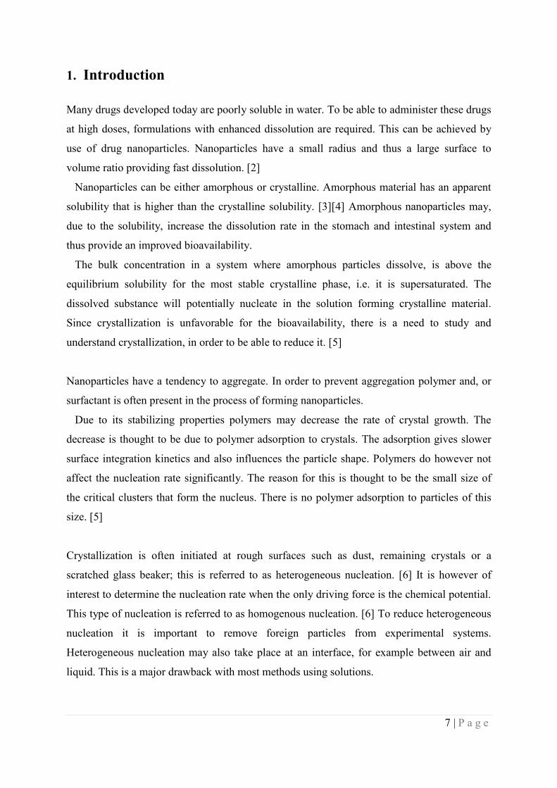
1. Introduction
Many drugs developed today are poorly soluble in water. To be able to administer these drugs
at high doses, formulations with enhanced dissolution are required. This can be achieved by
use of drug nanoparticles. Nanoparticles have a small radius and thus a large surface to
volume ratio providing fast dissolution. [2]
Nanoparticles can be either amorphous or crystalline. Amorphous material has an apparent
solubility that is higher than the crystalline solubility. [3][4] Amorphous nanoparticles may,
due to the solubility, increase the dissolution rate in the stomach and intestinal system and
thus provide an improved bioavailability.
The bulk concentration in a system where amorphous particles dissolve, is above the
equilibrium solubility for the most stable crystalline phase, i.e. it is supersaturated. The
dissolved substance will potentially nucleate in the solution forming crystalline material.
Since crystallization is unfavorable for the bioavailability, there is a need to study and
understand crystallization, in order to be able to reduce it. [5]
Nanoparticles have a tendency to aggregate. In order to prevent aggregation polymer and, or
surfactant is often present in the process of forming nanoparticles.
Due to its stabilizing properties polymers may decrease the rate of crystal growth. The
decrease is thought to be due to polymer adsorption to crystals. The adsorption gives slower
surface integration kinetics and also influences the particle shape. Polymers do however not
affect the nucleation rate significantly. The reason for this is thought to be the small size of
the critical clusters that form the nucleus. There is no polymer adsorption to particles of this
size. [5]
Crystallization is often initiated at rough surfaces such as dust, remaining crystals or a
scratched glass beaker; this is referred to as heterogeneous nucleation. [6] It is however of
interest to determine the nucleation rate when the only driving force is the chemical potential.
This type of nucleation is referred to as homogenous nucleation. [6] To reduce heterogeneous
nucleation it is important to remove foreign particles from experimental systems.
Heterogeneous nucleation may also take place at an interface, for example between air and
liquid. This is a major drawback with most methods using solutions.
8 | P a g e
Crystallization consists of two different processes, nucleation and crystal growth, usually
occurring simultaneously in a supersaturated solution. [5]
In classic nucleation theory, the main parameter of interest is the interfacial tension between
the crystal and the surrounding solution, γsl. The interfacial tension can be interpreted as the
free energy cost required creating a new surface between a solid and a liquid (per area unit).
When the supersaturation in a solution is high so is the crystallization rate. When lowering the
supersaturation, it will eventually reach a concentration where nucleation ceases but crystal
growth continues. The concentration range between this limit and the equilibrium solubility is
called the metastable zone. [5]
Attempts to determine the nucleation rate have previously been done for proteins,
pharmaceutical substances and different inorganic materials, using methods involving
nucleation in the vapor-liquid phase or measurements of the induction time, the time required
for formation of detectable crystals in liquids. [7][8][9]
Lately, attempts have been made to separate nucleation from crystal growth for proteins.
[10][11][12][13] Galkin and Vekilov used temperature to control the degree of
supersaturation during the nucleation process. In such experiments a supersaturated solution is
generated. After a predetermined time, the nucleation time, the temperature is lowered to
decrease the supersaturation into the metastable zone. This method has the advantage of
allowing a large number of experiments to be performed simultaneously with identical
conditions. The results can therefore be statistically evaluated, which is important since
nucleation is a stochastic process. [14]
Other attempts to determine the nucleation rate have also been made for the substance
Bicalutamide. [5] Lindfors et al. used dilution with a substance saturated solution to lower the
concentration into the metastable zone.
In this paper the methods developed by Galkin, Vekilov and Lindfors et al. has been
modified further in order to get more understanding of the nucleation process and to be able to
determine the nucleation rate with higher accuracy. This would convey information about the
interfacial tension and correspondence between experimental results and theory.
Crystal growth in supersaturated solutions has been studied previously by use of fluorescence.
[4][5] The same is valid in this paper, but different supersaturations are to be investigated.

9 | P a g e
The way of stabilizing the initial nanoparticles have also been altered in order to see how the
stabilization affects crystal growth in the experimental system. [5]
The experimental result gives information about the surface integration kinetics. Three
different theories have been used to evaluate the experimental results.
The -model describes growth as incorporation of monomers. The rate of incorporation can
be described by the surface integration factor, .
The other theoretical models describe crystal growth as a surface nucleation process. The
Hillig-Nielsen theory uses a polynuclear model to describe the growth from a supersaturated
solution. [15] The Obretenov interpolation model describes crystal growth by interpolating
mono- and poly nuclear growth mechanisms in a continuous mode. [16]
Crystal dissolution in water has previously been investigated by Lindfors et. al. [4] Here, the
same has been done for a range of undersaturations. The aim was to determine that previous
results indicating that the dissolution process is diffusion controlled, i.e. =0, were correct
and applying for all tested substances, regardless of the concentration in the solution.

10 | P a g e
2. Theory
Knowledge of the crystallization process is rather poor regarding the nucleation and crystal
growth separately since the two processes normally occur simultaneously.
The theory below is based on classic nucleation theory and spherical symmetry.
2.1 Nucleation
In a supersaturated solution crystals will eventually form in order to minimize the free energy
in the system. Clusters are formed when free monomers, M, by diffusion meet and form
dimers, M2. Dimers can then either grow by addition of further monomers giving trimers, M3,
or they can dissolve to free monomers again. The formation of clusters can be described by
the following equation:
(1)
The nucleation process has an energy barrier. Before the cluster reaches the critical size, R*, it
is a subcritical cluster with larger probability to dissolve since its existence is
thermodynamically unfavorable. When the size exceeds the critical radius, it becomes
supercritical and then it is thermodynamically favorable for the cluster to continue to grow.
A critical cluster has equal probability to grow and dissolve.
Nucleation from a liquid phase can be described by considering the free energy change of
forming a solid sphere of radius, R.
(2)
where ΔG is the free energy change, nc is the number of aggregating molecules, kB is the
Boltzmann constant, T is the temperature in Kelvin, C is the molar concentration, S0 is the
intrinsic solubility, and γsl is the interfacial tension, between a solution and a crystal.
11 | P a g e
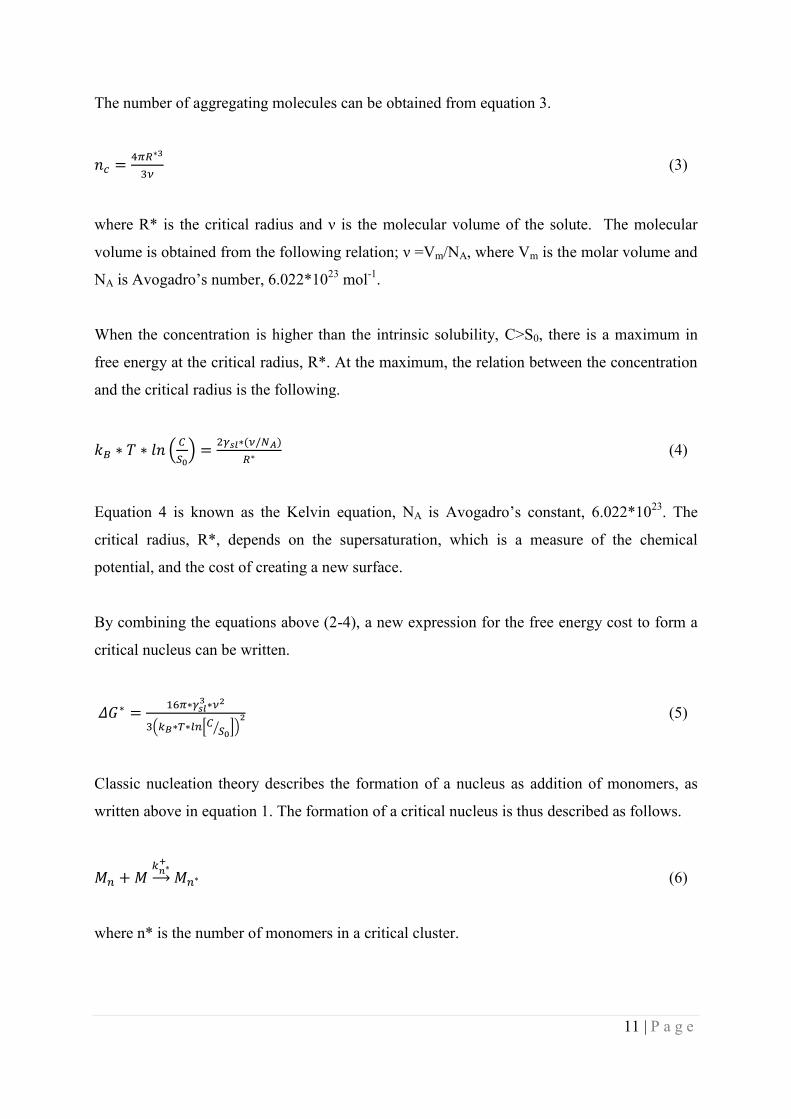
The number of aggregating molecules can be obtained from equation 3.
(3)
where R* is the critical radius and ν is the molecular volume of the solute. The molecular
volume is obtained from the following relation; ν =Vm/NA, where Vm is the molar volume and
NA is Avogadro’s number, 6.022*1023
mol-1
.
When the concentration is higher than the intrinsic solubility, C>S0, there is a maximum in
free energy at the critical radius, R*. At the maximum, the relation between the concentration
and the critical radius is the following.
(4)
Equation 4 is known as the Kelvin equation, NA is Avogadro’s constant, 6.022*1023
. The
critical radius, R*, depends on the supersaturation, which is a measure of the chemical
potential, and the cost of creating a new surface.
By combining the equations above (2-4), a new expression for the free energy cost to form a
critical nucleus can be written.
(5)
Classic nucleation theory describes the formation of a nucleus as addition of monomers, as
written above in equation 1. The formation of a critical nucleus is thus described as follows.
(6)
where n* is the number of monomers in a critical cluster.
12 | P a g e
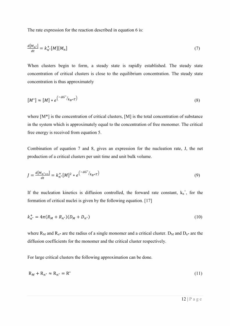
The rate expression for the reaction described in equation 6 is:
(7)
When clusters begin to form, a steady state is rapidly established. The steady state
concentration of critical clusters is close to the equilibrium concentration. The steady state
concentration is thus approximately
(8)
where [M*] is the concentration of critical clusters, [M] is the total concentration of substance
in the system which is approximately equal to the concentration of free monomer. The critical
free energy is received from equation 5.
Combination of equation 7 and 8, gives an expression for the nucleation rate, J, the net
production of a critical clusters per unit time and unit bulk volume.
(9)
If the nucleation kinetics is diffusion controlled, the forward rate constant, kn+, for the
formation of critical nuclei is given by the following equation. [17]
(10)
where RM and Rn* are the radius of a single monomer and a critical cluster. DM and Dn* are the
diffusion coefficients for the monomer and the critical cluster respectively.
For large critical clusters the following approximation can be done.
(11)

13 | P a g e
The diffusion of monomers is much larger than diffusion of clusters, DM>>Dn*, from this
relation and equation 11, equation 10 can be simplified.
(12)
When combining equation 4, 5, 9 and 12, the expression for the nucleation rate is the
following:
(13)
As can be seen in this equation, the nucleation rate strongly depends on the interfacial tension
of the solid/liquid interface.
2.3 Crystal Growth
2.3.1 Surface integration model
In a supersaturated solution the transport of monomers to a particle surface is diffusion
controlled. This is true even with moderate stirring since there is a stagnant layer closest to the
particle surface. Through this layer only diffusion is possible.
It is assumed in the theory below that the clusters are spherical and that the monomers are of
negligible size compared to the clusters.
The concentration gradient in the steady-state diffusion field around a particle can be
described as the concentration difference between the bulk, Cb, and the surface of a thin
boundary layer outside the particle, divided by the radius of the particle, (Cb-C')/R*
To determine concentration at the surface of the crystal the following equation can be used.
(14)

14 | P a g e
Where S0 is the intrinsic solubility and
(15)
in equation 15 is a surface integration factor.
The chemical potential difference between the crystal surface and the solution is the driving
force for crystal growth. The chemical potential difference can be received from the following
equation:
(16)
Where ΔμSurface is the difference in chemical potential between the bulk and the crystal
surface.
Fick’s first law can describe the flow of material into the crystal. The process is diffusion
controlled and in one dimension, this law is given by:
(17)
JD is the flow of monomers, D0 is the intrinsic diffusion coefficient for monomers and dC/dx is
the concentration gradient.
In three dimensions and with the assumption that C’ is equal to the solubility on the surface of
the particle this law becomes
where dM/dt is the molar flow of monomers to the particle surface, A is the surface area,
C(R) is the concentration gradient as a function of distance from the center of the particle,
and S(R) is the concentration at the surface of the particle, that is equal to the solubility, S0.

15 | P a g e
Crystal growth is not entirely controlled by diffusion. When a monomer reaches the crystal
surface it has to find a suitable site for attachment and create or break bonds. This is known as
surface integration and modeled as a thin boundary layer through which monomers must pass,
resulting in a slower net flow of monomers to the surface.
The transport through the imagined layer can be said to be proportional to a surface
integration factor, k+, and the area of the layer. By defining the surface integration constant
λ=D0/k+, equation 18 can be rewritten:
(19)
Where, ψ=r/(λ+R).
Equation 19 can be further reformulated into
(20)
If R>>λ, the growth process is controlled by diffusion and if, and if λ>>R the growth will be
limited by surface integration.
2.3.2 Surface nucleation
Another approach to the mechanisms behind crystal growth is the Hillig-Nielsen theory.
According to this theory the growth of crystals occur by two-dimensional nucleation, so
called surface nucleation. [6]
Surface nucleation occurs through nucleation and growth of layers on the crystal surface
and can be compared to surface condensation events. [18] The growth occurs by formation of
two-dimensional nuclei on the existing crystal surface and lateral spreading of the new crystal
layer. According to the Hillig-Nielsen theory, multinuclear growth takes place. This means
that several nuclei can be formed simultaneously, and that one layer does not have to be
entirely covered before new nuclei are formed. [19]

16 | P a g e
To model crystal growth by multilayer 2D-nucleation, the flow of monomers to the surface
has to be considered at first. The flow was derived in section 2.3 and is be described by
equation 17.
Gibbs free energy for surface nucleation is described by:
(21)
The first term corresponds to the edge work of increasing the 2D nucleus circumference, the
second term is the free energy gained by incorporating a monomer in to the 2D nuclei.
The free energy for creation of a critical two dimensional cluster can be derived from the
equation above.
(22)
The number of monomers in the critical 2D nuclei is thus
(23)
Equation 22 can by use of equation 23 and the relation n=R2/a
2 be reformulated into
(24)
Further, equation 24 can be reformulated into the following
(25)
The total rate of crystal growth is also dependent of the rate of lateral spreading of the 2D
nuclei.

17 | P a g e
Kink positions, positions where the surface energy is the same if a monomer is added or
removed are the positions where monomers are incorporated into a crystal. According to the
Hillig-Nielsen theory, the net flow of monomers to kink positions is:
(26)
Where νin is the frequency by which molecules are incorporated into the crystal. Assuming
that kink positions are found at the edge of formed 2D nuclei, at an average distance χ0 from
one another, the probability that a 2D nuclei of radius R will gain a monomer is the following.
(27)
The average distance between the kink positions can be described by the equation below.
(28)
By inserting equation 28 into equation 27, the following expression for the rate of monomer
integration is derived.
(29)
By combining the lateral spreading rate and the rate of 2D nucleation, the total rate of crystal
growth can be described according to equation, 30.
(30)
There are two parameters in the equation that are to be determined for each substance; sl is
the apparent surface tension and νin is the integration frequency (Hz). [15]

18 | P a g e
The complete derivation can be found in Generalized Hillig-Nielsen Theory, for crystalline
nanoparticles, by Rasmus Persson, see reference 19.
2.3.3 Obretenov interpolation
Obretenov describes crystal growth by 2D nucleation as a process that can occur either by
mono- or multinuclear growth, depending on the supersaturation of the solution. The growth
rate is described by a unified expression that combines known equations for mono- and
multinuclear growth. [16]
The growth rate for mononuclear crystal growth is described by equation 31.
(31)
Where 2R is the monolayer height for spheres constructing a layer, J2D is the rate of 2D
nucleation and a is the crystal face area.
For the polynuclear growth mechanism the statistical theory of Kolmogorov-Avrami-Evans is
incorporated in the theory. Due to the statistics used, the multinuclear growth expression is
only valid for a sufficiently large number of nuclei per monolayer. The general form of the
growth rate expression is:
(32)
Where w is the spreading velocity of the monoatomic step and is a constant numerical
factor close to unity, 0.97, when polynuclear growth described by Hillig-Nielsen is used. [16]
In the middle region of the crystal growth curve, between mononuclear growth (beginning)
and polynuclear growth (the end), each monolayer will be formed by several nuclei. The
growth rate can thus be described by equation 33.
(33)

19 | P a g e
Where n is the average number of nuclei taking part in the formation of one monolayer.
n can be determined by the following equation.
(34)
The steady state growth rate for combined mono- and multinuclear growth can thus be
describes by the following equation. [16]
(35)
2.4 Secondary nucleation
Classic nucleation theory does not take into account the effects of existing crystals in the
solution, so called secondary nucleation. [20] Large crystals are thought to stabilize small
unstable clusters of monomers by van der Waals interactions when in close proximity and
thus facilitate nucleation. [21]
Van der Waals forces between particles of the same material have stabilizing effects. Large
crystals are thus thought to have stabilizing effects on subcritical nuclei, lowering the ΔG*
and increasing the rate of forming supercritical nuclei. This secondary nucleation effect is
given by
(36)
where A121 is the Hamaker constant and l is the distance between the surface of the large
crystal and the cluster. [21]
For a large crystal to stabilize a subcritical nucleus the distance between them has to be very
small. Taking the short distance into account, the effect of surface integration on
concentration profiles outside crystals becomes very important. Diffusion controlled growth
of a particles means that the concentration very close to the surface of the large crystal is
equal to the intrinsic solubility. This conveys that only monomers can exist in the solution
20 | P a g e
close to the surface and thus the effect of secondary nucleation would not be possible. If on
the other hand, crystal growth is controlled by surface integration, the concentration profile is
altered. The concentration very close to the crystal surface is then no longer equal to the
intrinsic solubility, but higher. Subcritical nuclei will be able to come in close proximity of
the large crystal and thus they can be stabilized for further growth. [21]
The stabilization of one subcritical nucleus results in more crystals formed that in turn can
stabilize further subcritical nuclei resulting in a chain reaction. The effects of the stabilization
on the critical radius, R*, depends on the distance to the large crystal. [21]
Other theories exist as well. Molecular build-up on the surface of the parent crystal that has
not been well incorporated in the crystal lattice might be removed into the supersaturated
solution where it will have the opportunity to grow. Diffusion effects or the shearing action of
a stirred solution might apply force enough to remove the layer.
The parent crystal might also grow in a way, with dendrites, that the shearing action of the
solution can tear off small clusters from the crystal surface and these can then develop in the
supersaturated solution. [20]
2.5 Crystal dissolution
The process of crystal dissolution is in theoretical terms described the same way as the crystal
growth. Since it is the reverse of crystal growth, the diversion from diffusion controlled
dissolution rate is modeled by a surface disintegration step where the detachment rate
constant, k- is included. [4]
21 | P a g e
3. Experiments
3.1 Substances
Three model substances were used in the performed experimental studies. Bicalutamide,
Linaprazan and Felodipine were provided from Astra Zeneca and used without any further
purification.
3.1.1 Characteristics
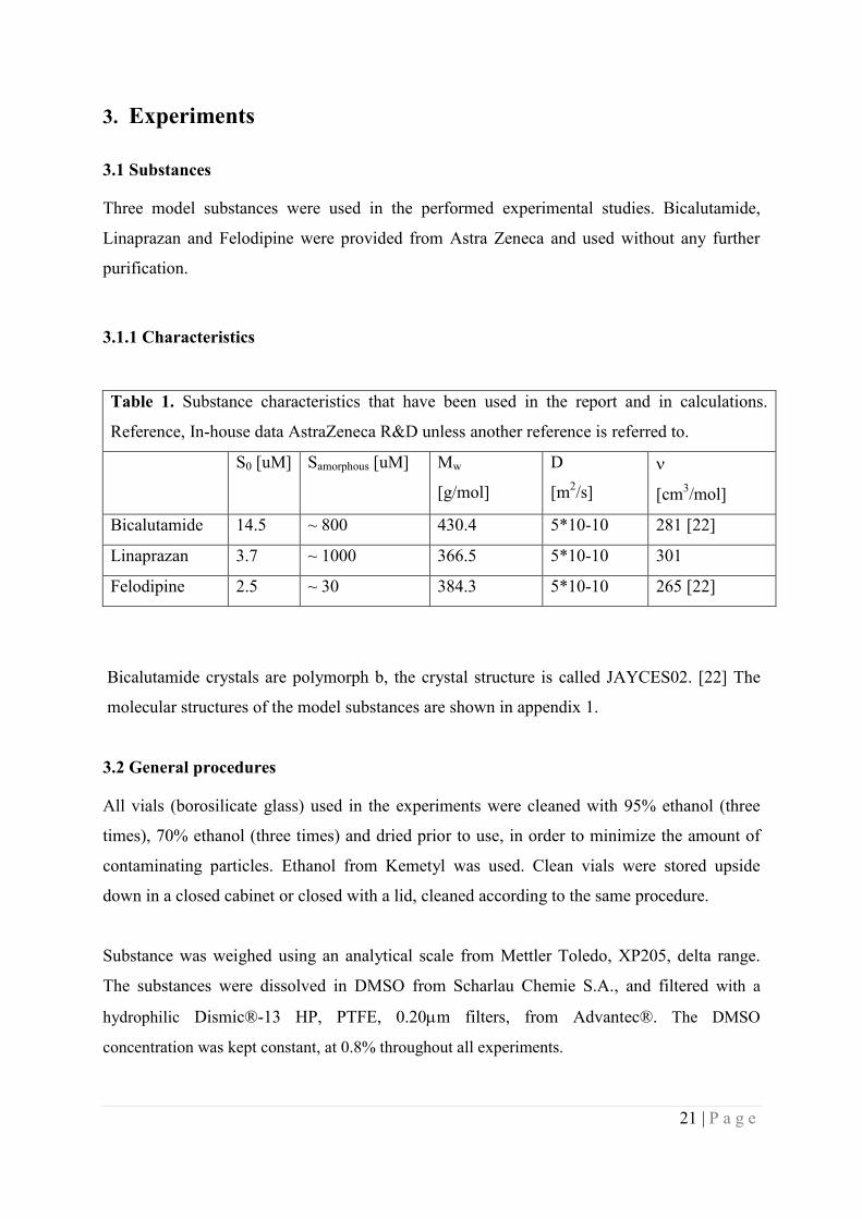
Bicalutamide crystals are polymorph b, the crystal structure is called JAYCES02. [22] The
molecular structures of the model substances are shown in appendix 1.
3.2 General procedures
All vials (borosilicate glass) used in the experiments were cleaned with 95% ethanol (three
times), 70% ethanol (three times) and dried prior to use, in order to minimize the amount of
contaminating particles. Ethanol from Kemetyl was used. Clean vials were stored upside
down in a closed cabinet or closed with a lid, cleaned according to the same procedure.
Substance was weighed using an analytical scale from Mettler Toledo, XP205, delta range.
The substances were dissolved in DMSO from Scharlau Chemie S.A., and filtered with a
hydrophilic Dismic®-13 HP, PTFE, 0.20m filters, from Advantec®. The DMSO
concentration was kept constant, at 0.8% throughout all experiments.
Table 1. Substance characteristics that have been used in the report and in calculations.
Reference, In-house data AstraZeneca R&D unless another reference is referred to.
S0 [uM] Samorphous [uM] Mw
[g/mol]
D
[m2/s]
[cm3/mol]
Bicalutamide 14.5 ~ 800 430.4 5*10-10 281 [22]
Linaprazan 3.7 ~ 1000 366.5 5*10-10 301
Felodipine 2.5 ~ 30 384.3 5*10-10 265 [22]

22 | P a g e
MilliQ water, from the Elix 3 system from Millipore, was used in the experiments and filtered
with hydrophilic Dismic®-13 HP, PTFE, 0.20m filters from Advantec® prior to use.
Pipettes from the Eppendorf Reference Series were used for all pipetting.
All experiments were performed at room temperature, without stirring and in darkness at
elevated experimental times.
3.3 pH adjustment
All experiments performed on Linaprazan contained 1M NaOH, from Sigma Aldrich. This
was done to keep the pH above the pKa of the molecule, to be certain that the molecule was
uncharged. [1] The experimental pKa is 6.1. [23]
3.4 Preparation of substance solutions
This procedure applies for supersaturated solutions, growth solutions and undersaturated
solutions.
The drug dissolved in DMSO was calmly added to water in a 10ml vial. Gentle mixing was
performed by turning the closed vessel three times, giving a solution with a final DMSO
concentration of 0.8(v/v) % and four milliliter supersaturated solution.
After creating the substance solution it was filtered to eliminate any solid material, such as
initial crystals. As written above, 0.2m hydrophilic PTFE filters were used for all
substances.
3.5 Filtration
The choice of filters was investigated by use of fluorescence.
Experiments were carried out in the same way as crystal growth experiments; see section
3.3.5, to see if the filter used had any affect. Different amount of water was filtered with two
different filters, PTFE and Millex- filters. Unfiltered water was used as reference.
23 | P a g e
3.6 Nanoparticles
3.6.1 Theoretical considerations
Crystalline nanoparticles, can effectively be prepared by use of precipitation-ultrasonication
method [24] or by wet milling. [25]
Precipitation means that the drug is solved, often an organic solvent. The solution is rapidly
added into a miscible non-solvent, usually an aqueous solution. [26] Use of ultrasound has
proved to be an efficient way to control the nucleation and crystallization process. The
mechanisms are thought to be cavitations and acoustic streaming. [24]
Milling is an attrition based way of making nanoparticles. The drug is dispersed in an
aqueous solution with suitable stabilizators. The dispersion is mixed with beads of for
example zirconium. The mixture is then milled and the procedure generates enough energy to
convert the drug crystals into nanoparticles. [25]
To prevent aggregation and have stable crystalline particles, stabilization is needed. This can
be received by steric hindrance and, or electrostatic stabilization.
Polymers are often used for steric stabilization, while surfactants often are used for
electrostatic stabilization. If both types are used simultaneously, it is called electrosterical
stabilization.
The stabilization, both type and specific species, that is suitable, depends on properties of
the substance that should crystallize. Charge, pKa, and hydrophilicity, logP, are the most
important properties to consider. [27] The stabilizer must of course have sufficient affinity for
the particles surface and it must also have a rather high diffusion rate in order to cover the
generated surface rapidly. [28]
A highly charged surface can often be properly stabilized by use of a polymer, while surfaces
with low charge might need a mixture of a polymer and a surfactant. [27]
Polymers are known to decrease crystal growth rate when stabilizing crystalline particles. The
decrease is thought to be due to polymer adsorption to the crystal giving slower surface
integration kinetics and it is thought to influence the particle shape too. Thus, when
experimentally investigating crystal growth it is important not to have polymers present
stabilizing the particles. [5] It is however not yet known how surfactants impact the growth
rate.

24 | P a g e
3.6.2 Preparation of nanoparticles
Several details in the process of making nanocrystals by use of the precipitation method and
ultrasound were evaluated in the previous work, Crystal nucleation of poorly soluble drugs, I.
Method development and initial experimental results. [1]
For Bicalutamide and Felodipine the ultrasonic treatment was performed in Biotage
microwave vials 2-5ml with an S2 from Covaris for the ultrasonic treatment.
Bicalutamide nanoparticles were prepared by addition of drug dissolved in DMSO to the
stabilizer solution, giving a final concentration of 1mM of Bicalutamide, 0,8% (v/v) of
DMSO and 0.1% (w/w) AOT, Dioctyl sulfosuccinate, Mw= 444.6g/mol. The drug was
rapidly added into the stabilizer solution when the ultrasonic treatment was just started.
Felodipine nanoparticles were prepared by addition of drug dissolved in DMSO, to a final
concentration of 0.5mM of Felodipine, 0.8% (v/v) DMSO and 0.1 % (w/w) AOT. The drug
was rapidly added to the stabilizer solution on an ultrasonic bath, Transsonic T460 from
Elma®, with fresh and degassed water. The solution was then rapidly transferred to the
Covaris S2 for ultrasonic treatment.
The protocols are attached, see appendix 2 and 4.
Linaprazan nanosuspension was prepared by wet milling. The substance was suspended in a
stabilizer solution giving 1.33 (w/w) % PVP (K30) and 0.067% (w/w) AOT and 10 (w/w) %
substance. The suspension was milled according to the procedure in appendix 3.
The substance concentration in the milled nanosuspension was determined to 101mM by
use of LC.
3.6.3 Size measurements
Size measurements were performed in the Mastersizer 2000, from Malvern, where the entire
particle size distribution is received. The refractive index was set to 1.59.
For Bicalutamide and Felodipine 18ml, 125M solution was injected and for Linaprazan
20L of high concentration, 101mM, was added to water in the sample cell.

25 | P a g e
If the nanoparticles were not freshly prepared, gentle mixing and ultrasonic treatment (30
seconds) was applied prior to the size measurement. This was done to disperse any aggregates
and receive a homogeneous sample.
3.7 Fluorescence
3.7.1 Theoretical considerations
When a molecule absorbs light or electromagnetic radiation it can be excited to a higher
energy level. As the molecule returns to its ground state light is emitted. The emitted light
normally has less energy than the excited light and thus it has a longer wavelength, according
to the equation below.
hchfE (37)
where h is Planck´s constant, f is the frequency, c is the speed of light and is the
wavelength.
At low concentration the intensity of the fluorescence light is generally proportional to the
concentration. This relation can be used when performing quantitative measurements on
fluorescent substances.
(38)
I is the fluorescence intensity, and [S] is the concentration of substance in the sample.
Due to quenching molecules in solution have lower fluorescence than molecules incorporated
in crystals. In favorable cases the intensity from the supersaturated solution can be neglected
and the intensity from the sample is thus proportional to the fluorescence of the crystals.
(39)
26 | P a g e
3.7.2 Fluorescence measurements
The experiments that have been carried out and are described in this report have its foundation
in experiments and method development that was presented in Nucleation of poorly soluble
drugs, I. Method development and initial experimental results. [1]
All fluorescence measurements were performed in quarts cuvette from Hellma, prior to use
washed thoroughly with 99.5% ethanol (shaking with fresh ethanol ten times), dried with
nitrogen gas and left upside down when stored.
The measurements were performed on two milliliter samples using the LS 55 Luminescence
Spectrometer from Perkin Elmer™ Instruments.
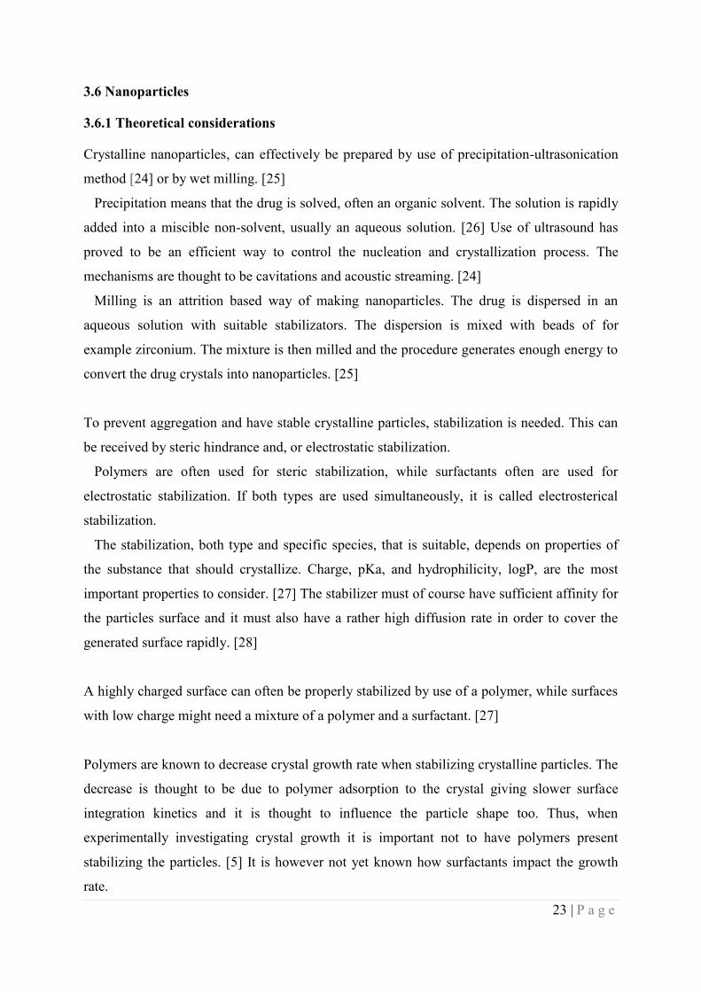
Information about excitation and emission wavelengths for the substances was already
known for Bicalutamide and Felodipine. [1] For Linaprazan absorbance measurements and
emission and excitation scans were performed to find wavelengths where the concentration
dependence is linear for crystals and the influence of substance in solution is small enough to
be neglected.
Table 2. Settings for growth fluorescence measurements of the studied substances.
Excitation
nm
Excitation
slit width,
Growth
experiments
[nm]
Excitation
slit width,
Dissolution
experiments
[nm]
Emission
[nm]
Emission
slit width,
Growth
experiments
[nm]
Emission
slit width,
Dissolution
experiments
[nm]
Bicalutamide 234 5 323 2.5
Linaprazan 300 5 378 2.5
Felodipine 370 2.5 430 2.5
3.8 Liquid Chromatography
Liquid chromatography, at a Waters system 2695 Separations module with a Waters 2998
Photodiode Array Detector, was used to perform quantitative measurements of the
concentration of substance in samples in 1.5ml LC-vials from Waters.
27 | P a g e
For Bicalutamide an XTerra RP8 column with a particle size of 3.5M and column
dimensions 3.9*100mm was used. The mobile phase used was 56% H2O, 44% AcN,
Acetonitrile, from Fisher Scientific and 10mM formic acid, from Merck, with a flow rate of
0.8ml/min.
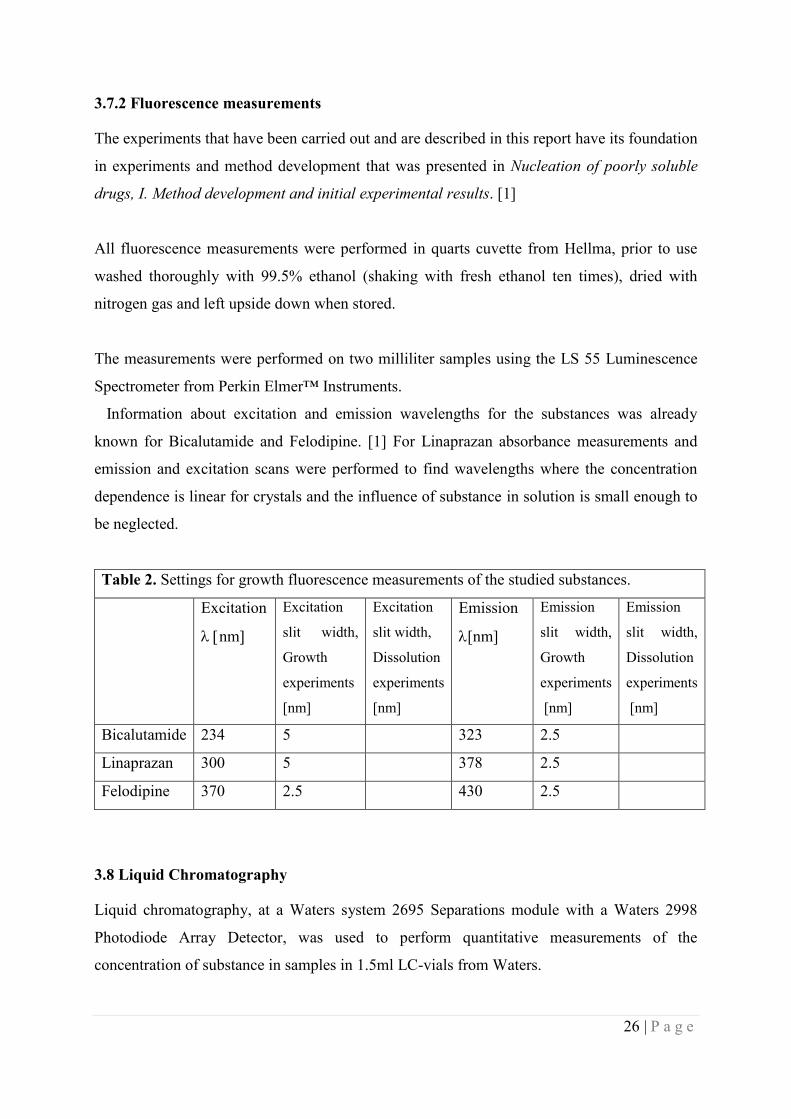
For Linaprazan an XTerra RP8 column with a particle size of 3.5M and column dimensions
3.9*100mm was used. The mobile phase had the following components; A: 80% 0.1M
sodium phosphate buffer at pH 6, from Sigma Aldrich and 20% AcN, and B contained 100%
AcN. The flow rate was 0.8ml/minute and the gradient in table 3 was used.
Table 3. Gradient used for liquid chromatography of Linaprazan. The flow rate was
0.8ml/min. Mobile phase A contains 80% 0.1M sodium phosphate buffer pH 6, and 20%
AcN. Mobile phase B contains 100% AcN.
Time [minute] / component A [%] B [%]
0 90 10
4 60 40
5 40 60
6 90 10
For Felodipine an XBridge C18 column with a particle size of 3.5M and column dimensions
3.0*100mm was used. The mobile phase used was 55% AcN, 45% H2O and 0.025% trifluoric
acid, TFA, from Merck, with a flow rate of 1.0 ml/min.
3.9 Crystal growth experiments
3.9.1 Starting point
Crystal growth experiments have been performed previously by Lindfors et al [4] and in the
previous thesis work. [1] The experiments were performed by addition of a supersaturated
solution to pre-formed nanocrystals.
The same method has been used here, but with PTFE-filters and also for Linaprazan.
28 | P a g e
3.9.2 Growth experiments
Growth experiments were performed by addition of nanocrystals, to the bottom of the rinsed
quarts cuvette from Hellma, giving 10% (mol/mol) crystalline material in the final solution
for Bicalutamide and Felodipine and 7.1% (mol/mol) for Linaprazan.
Solution of a certain supersaturation was added rapidly and the fluorescence measurement
was then performed.
The settings used for each substance are shown in table 2. The protocols for the growth
experiments are attached see appendix 5, 6 and 7.
3.9.3 Metastable zone for growth
As for crystal nucleation there is a metastable zone for crystal growth. To determine the
metastable zone, growth experiments with solutions of low concentration was conducted for
the chosen time range (3 hours). Where no increase in intensity was seen during this time, the
limit of the metastable zone was determined.
3.10 Crystal Dissolution experiments
3.10.1 Starting point
Dissolution experiments have been performed previously on Felodipine by Lindfors et al. [4]
The experiments were performed by addition of an under-saturated solution to pre-formed
nanocrystals in a quarts cuvette, measuring the fluorescence.
3.10.2 Crystal Dissolution
The crystal dissolution experiments were performed by addition of nanocrystals to the bottom
of the rinsed quarts cuvette from Hellma. Solutions with substance concentration below
saturation were added rapidly to the running fluorescence measurements.
The total substance concentration varied between 3 and 90% of the solubility, with constant
crystal concentration in all experiments.
The settings used for each substance are shown in table 2. The protocols for the dissolution
experiments are attached see appendix 8, 9 and 10.
29 | P a g e
3.11 Crystal nucleation experiments
3.11.1 Starting point
As written above, the Vekilov and Galkin method, modified by Lindfors et al and further in
the previous thesis work, has been the starting point for these experiments. The aim was to
develop the method and to investigate more substances and supersaturations.
The method developed in the previous thesis work, was in a simplified way, the following
for Bicalutamide. A supersaturated solution was created as described above. The
supersaturated solution was filtered into a PVP coated polystyrene reagent reservoir. The
solution was left ambient at room temperature during the nucleation time, after which the
solution was transferred to a 96 microwell plate pre-filled with a substance saturated solution
to lower the concentration into the metastable zone. In the metastable zone crystals were
allowed to grow to detectable size (72 hours).
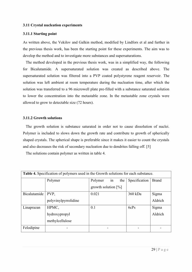
3.11.2 Growth solutions
The growth solution is substance saturated in order not to cause dissolution of nuclei.
Polymer is included to slows down the growth rate and contribute to growth of spherically
shaped crystals. The spherical shape is preferable since it makes it easier to count the crystals
and also decreases the risk of secondary nucleation due to dendrites falling off. [5]
The solutions contain polymer as written in table 4.
Table 4. Specification of polymers used in the Growth solutions for each substance.
Polymer Polymer in the
growth solution [%]
Specification Brand
Bicalutamide PVP,
polyvinylpyrrolidine
0.021 360 kDa Sigma
Aldrich
Linaprazan HPMC,
hydroxypropyl
methylcellulose
0.1 6cPs Sigma
Aldrich
Felodipine - - - -

30 | P a g e
3.11.3 Antivibration table
All nucleation experiments and metastable zone experiments have been performed on an
antivibration table, from Technical Manufacturing Corporation, to decrease disturbance. [2]
3.11.4 Metastable zone experiments
Supersaturated solutions of different concentrations were prepared as described above. After
filtration, the solutions were left for a certain time, 72 hours, in four milliliter vials. The
solutions were stored in dark on the anti-vibration table.
After the nucleation time, the solutions were filtered to remove crystals and the
concentration of the solution was determined by use of LC.
For Felodipine the metastable zone experiments were performed with nucleation time from
three days to 21 days. Three different types of vials were tested. Borosilicate glass,
borosilicate glass coated with substance from nanosuspension and silanized glass.
3.11.5 Coating of vials
Felodipine nanosuspension was prepared as written above. The suspension was diluted to
25M with water. The solution was added to clean 4 ml vials, 3.5 ml per vial, and they were
put on a shaking table for five days and turned upside down daily.
After the coating process the vials were washed thoroughly with water and dried prior to
use.
3.11.6 Coating of plates
All polystyrene material was coated with polymer. This was done in order to minimize
interactions with the material, and thus reduce possibilities of heterogeneous nucleation and
absorption of substance to the polystyrene. [1] PVP was used for experiments performed on
Bicalutamide and HPMC was used for experiments with Linaprazan.
The 96 microwell plates, from NuncTM
Brand Products, were coated according to the
following procedures. For plates used for Bicalutamide 1% (w/w) PVP, 360kDa, was used
31 | P a g e
and for plates where Linaprazan was used 1% HPMC (6 cPs) was used. The protocols for
these procedures are attached, see appendix 11 and 12.
3.11.7 Crystal nucleation experiments
Supersaturated solutions were prepared as described above and filtered into 4 ml vials where
the solution was left for the decided nucleation time. The nucleation was terminated by
moving a certain amount of the supersaturated solution to wells on a 96-well plate, by use of a
manual pipette. The plate was pre-filled with growth solution used to dilute the sample into
the metastable zone.
The supersaturated solution was handled carefully and added in a controlled manner, followed
by careful mixing by use of the pipette.
The samples were after dilution left in dark on the anti-vibration table for the growth time
when the crystals grew to detectable size. The protocol for the experiment is attached, see
appendix 11 and 12.
Results have to this point been received for one concentration for Bicalutamide and initial
experiments have been conducted on Linaprazan.
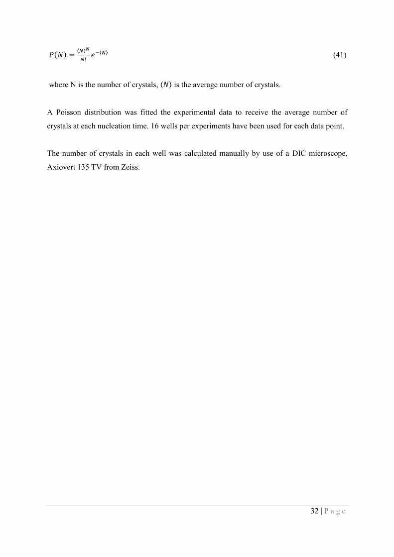
3.11.8 Evaluation of nucleation experiments
The nucleation rate, J, can experimentally be calculated by the following equation
(40)
where V is the volume of the initial supersaturated solution prior to dilution, and Δt is the
nucleation time. For short nucleation times the nucleation rate can be determined for a certain
supersaturation, assuming that the nuclei that are formed do not change the bulk
concentration significantly. Assuming that the nucleation of each crystal is independent of
other crystals, the stochastic nucleation process can be described by a Poisson distribution.
[5]
32 | P a g e
(41)
where N is the number of crystals, is the average number of crystals.
A Poisson distribution was fitted the experimental data to receive the average number of
crystals at each nucleation time. 16 wells per experiments have been used for each data point.
The number of crystals in each well was calculated manually by use of a DIC microscope,
Axiovert 135 TV from Zeiss.
33 | P a g e
Time [sec.]
0 10 20 30 40
Inte
nsity
0
100
200
300
400
500
600
4. Results and discussion
4.1 General results
4.1.1 Effect of filters used to filter supersaturated solutions
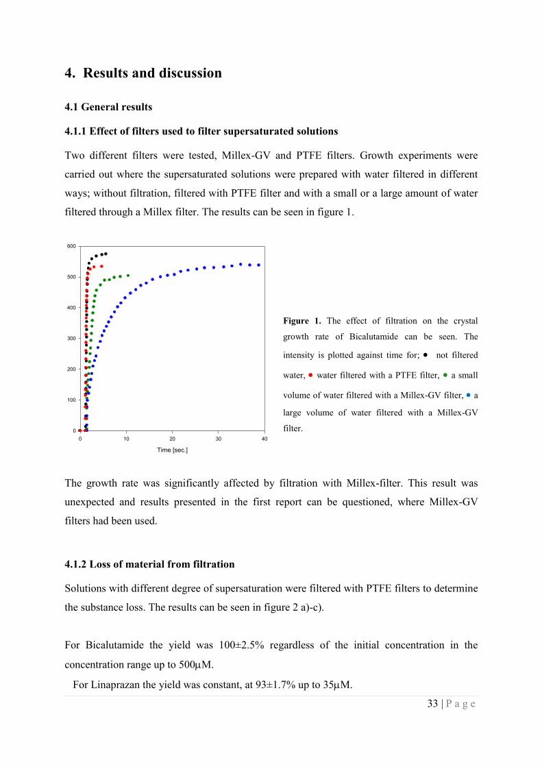
Two different filters were tested, Millex-GV and PTFE filters. Growth experiments were
carried out where the supersaturated solutions were prepared with water filtered in different
ways; without filtration, filtered with PTFE filter and with a small or a large amount of water
filtered through a Millex filter. The results can be seen in figure 1.
Figure 1. The effect of filtration on the crystal
growth rate of Bicalutamide can be seen. The
intensity is plotted against time for; not filtered
water, water filtered with a PTFE filter, a small
volume of water filtered with a Millex-GV filter, a
large volume of water filtered with a Millex-GV
filter.
The growth rate was significantly affected by filtration with Millex-filter. This result was
unexpected and results presented in the first report can be questioned, where Millex-GV
filters had been used.
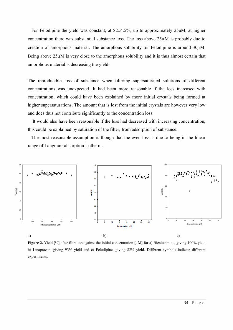
4.1.2 Loss of material from filtration
Solutions with different degree of supersaturation were filtered with PTFE filters to determine
the substance loss. The results can be seen in figure 2 a)-c).
For Bicalutamide the yield was 100±2.5% regardless of the initial concentration in the
concentration range up to 500M.
For Linaprazan the yield was constant, at 93±1.7% up to 35M.
34 | P a g e
For Felodipine the yield was constant, at 82±4.5%, up to approximately 25uM, at higher
concentration there was substantial substance loss. The loss above 25M is probably due to
creation of amorphous material. The amorphous solubility for Felodipine is around 30M.
Being above 25M is very close to the amorphous solubility and it is thus almost certain that
amorphous material is decreasing the yield.
The reproducible loss of substance when filtering supersaturated solutions of different
concentrations was unexpected. It had been more reasonable if the loss increased with
concentration, which could have been explained by more initial crystals being formed at
higher supersaturations. The amount that is lost from the initial crystals are however very low
and does thus not contribute significantly to the concentration loss.
It would also have been reasonable if the loss had decreased with increasing concentration,
this could be explained by saturation of the filter, from adsorption of substance.
The most reasonable assumption is though that the even loss is due to being in the linear
range of Langmuir absorption isotherm.
a) b) c)
Figure 2. Yield [%] after filtration against the initial concentration [M] for a) Bicalutamide, giving 100% yield
b) Linaprazan, giving 93% yield and c) Felodipine, giving 82% yield. Different symbols indicate different
experiments.
Concentration [M]
0 5 10 15 20 25 30
Yie
ld [
%]
0
20
40
60
80
100
Initial concentration [M]
0 100 200 300 400 500
Yie
ld [
%]
0
20
40
60
80
100
120

35 | P a g e
4.2 Crystal growth and dissolution experiments
4.2.1 Preparation of nanocrystals
To obtain good experimental data that can be compared with theory, the experimental systems
were designed to be as unaffected by additives as possible. One way of achieving this was to
try to produce nanoparticles that had reasonable stability, without polymeric stabilizer present.
This was achieved for Bicalutamide and Felodipine, but to prepare nanoparticles of
Linaprazan without polymer became quite a challenge.
For unknown reasons it was not possible to measure growth on Linaprazan particles
stabilized only with surfactant, even though they seemed to be of reasonable size and stability.
Milling was thus used to get Linaprazan nanoparticles, stabilized with both surfactant and
polymer. The concentration of stabilizer is however reasonably low.
Nanocrystals were evaluated with focus on size and stability. The particle size and size
distribution were measured several times after the production to make sure that the particles
were of reasonable size and stability.
Particles with intensity mean size up to 300 nm was accepted in these experiments.
The Bicalutamide particles had good stability for at least 14 days. The volume weighted mean
diameter was 137nm, and the entire distribution can be seen in appendix 13.
The measurement data has been edited, due to a small signal at larger size. The results
before the edit can be seen in appendix 14.
Milled Linaprazan particles had very good stability. The volume weighted mean diameter was
156nm, and the entire distribution can be seen in appendix 15.
The measurement data has been edited, due to a small signal at larger size. The results
before the edit can be seen in appendix 16. The editing was justified since nothing was
expected to be seen at the size, air bubbles might be a reasonable explanation.
Felodipine particles were stable up to between 24 and 48 hours. The volume weighted mean
diameter was 181nm, and the size distribution can be seen in appendix 17.
The measurement data has been edited, due to a small signal at larger size. The results from
before the edit can be seen in appendix 18.

36 | P a g e
2 4 6 8 10 12 14 16 18 20
0
100
200
300
400
500
600
Concentration [m]
Inte
nsity
The editing was justified since nothing was expected to be seen at the size. A reasonable
explanation might be air bubbles or contamination. The latter is strengthened since the
unexpected larger size particles are seen for all substances.
4.2.2 Fluorescence scan
The excitation wavelength for Linaprazan was chosen by looking at the absorbance curve
showing a maximum at 300nm, thus it is certain that it is the correct substance that is being
looked at in the experiments. Then an emission scan was performed, see appendix 19, from
this data the graph below was constructed.
Figure 3. Result from fluorescence measurements on
Linaprazan. The intensity is plotted against the sample
concentration for supersaturated solutions ■ and crystals
♦. Excitation at 300 nm and measuring the emission at 378
nm.
The fluorescence measurements on Linaprazan gave linearity for the crystals and low
influence from solution when excitation took place at 300 nm (5nm slit width) and the
emission was measured at 378 nm (2.5 nm slit width).
Similar, linear results have previously been obtained for Bicalutamide and Felodipine. [1]
4.2.3 Crystal dissolution
The crystal dissolution experiments were performed as described in section 3.10.2. The results
were normalized and display fraction of crystalline material as a function of time.
All results are shown in appendix 20, 21 and 22. The results and calculations for the highest
and lowest concentrations are presented for all substances below.
37 | P a g e
Time [seconds]
0 20 40 60 80 100 120
Fra
ctio
n c
rysta
lline
mate
rial
0.00
0.02
0.04
0.06
0.08
0.10
0.12
Time [minutes]
0 20 40 60 80 100 120
Fra
ctio
n c
rysta
lline
mate
rial
0.0
0.2
0.4
0.6
0.8
1.0
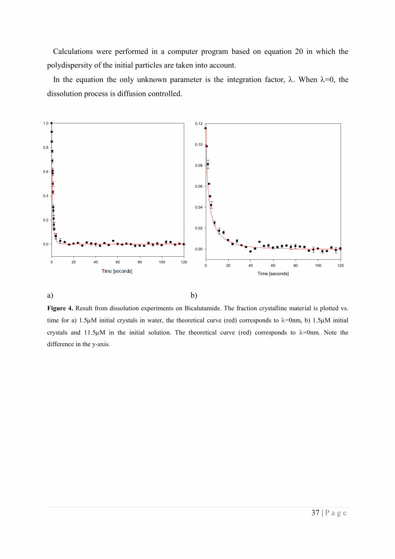
Calculations were performed in a computer program based on equation 20 in which the
polydispersity of the initial particles are taken into account.
In the equation the only unknown parameter is the integration factor, . When =0, the
dissolution process is diffusion controlled.
a) b)
Figure 4. Result from dissolution experiments on Bicalutamide. The fraction crystalline material is plotted vs.
time for a) 1.5M initial crystals in water, the theoretical curve (red) corresponds to =0nm, b) 1.5M initial
crystals and 11.5M in the initial solution. The theoretical curve (red) corresponds to =0nm. Note the
difference in the y-axis.

38 | P a g e
a) b)
Figure 5. Result from dissolution experiments on Linaprazan. The fraction crystalline material is plotted vs. time
for a) 0.1M initial crystals in water, the theoretical curve (red) corresponds to =0nm and (blue) m, b)
0.1M initial crystals and 1.15M in the initial solution. The theoretical curve (red) corresponds to =0nm and
(blue) m. Note the difference in the y-axis.
a) b)
Figure 6. Result from dissolution experiments on Felodipine. The fraction crystalline material is plotted vs. time
for a) 0.2M initial crystals in water, the theoretical curve (red) corresponds to =0nm, b) 0.2M initial crystals
and 1.6M in the initial solution. The theoretical curve (red) corresponds to =0nm. Note the difference in the
y-axis.
0 20 40 60 80 100 120 140 160
0.00
0.02
0.04
0.06
0.08
0.10
0.12
Time [seconds]
Fra
ctio
n c
rysta
lline
mate
rial
Time [seconds]
0 20 40 60 80 100 120 140 160
Fra
ction c
rysta
lline m
ate
rial
0.0
0.2
0.4
0.6
0.8
1.0
Time [seconds]
0 20 40 60 80 100 120 140
Fra
ctio
n c
rysta
llin
e m
ate
ria
l
0.0
0.2
0.4
0.6
0.8
1.0
0 20 40 60 80 100 120 140
0.00
0.02
0.04
0.06
0.08
Time [seconds]
Fra
ction c
rysta
lline m
ate
rial

39 | P a g e
The results agree well with theory. Deviation between experimental results and theoretical
results are mainly seen for Linaprazan. This is likely due to stabilization with polymer, and
perhaps also a small error in the solubility. The solubility of Linaprazan was investigated; the
previously determined solubility gave experimental dissolution that was faster than diffusion
controlled dissolution. Since this is impossible, the solubility was questioned and thus
measured in-house to get reliable data. The solubility of Linaprazan was determined to
3.7M, compared to 1.5M from previous data.
The same was also seen for Felodipine, but the solubility that made the experiments concur
with the theory was within the margin of error of the known solubility and the edited value
has thus been used throughout the entire report. The previous value was 2.1±0.5M, when
evaluating the dissolution data from Felodipine it became clear that the rate of dissolution
corresponded to a higher solubility. The solubility that gave the best agreement was 2.5M,
and since this is within the margin of error this value was accepted as the correct.
4.2.4 Growth experiments
Growth experiments were performed as described in section 3.3.5. The results were
normalized and display fraction of crystalline material as a function of time.
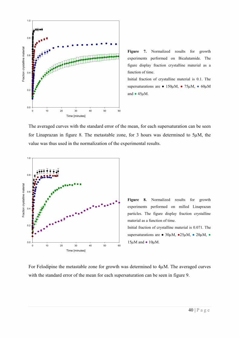
Normalized average curves with the standard error of the mean are to be seen for
Bicalutamide in figure 7. The metastable zone, the concentration range where no increase in
fluorescence was detected for 3 hours, was investigated. It was concluded that 17M was the
limit for Bicalutamide. This value was thus used in the normalization of the experimental
results.
It can clearly be seen in the figure that the rate of growth decreases with lower
supersaturations.
40 | P a g e
Figure 7. Normalized results for growth
experiments performed on Bicalutamide. The
figure display fraction crystalline material as a
function of time.
Initial fraction of crystalline material is 0.1. The
supersaturations are ● 150M, ● 75M, ● 60M
and ● 45M.
The averaged curves with the standard error of the mean, for each supersaturation can be seen
for Linaprazan in figure 8. The metastable zone, for 3 hours was determined to 5M, the
value was thus used in the normalization of the experimental results.
Figure 8. Normalized results for growth
experiments performed on milled Linaprazan
particles. The figure display fraction crystalline
material as a function of time.
Initial fraction of crystalline material is 0.071. The
supersaturations are ● 30M, ●25M, ● 20M, ●
15M and ● 10M.
For Felodipine the metastable zone for growth was determined to 4M. The averaged curves
with the standard error of the mean for each supersaturation can be seen in figure 9.
Time [minutes]
0 10 20 30 40 50 60
Fra
ction c
rysta
lline m
ate
rial
0.0
0.2
0.4
0.6
0.8
1.0
Time [minutes]
0 10 20 30 40 50 60
Fra
ction c
rysta
lline m
ate
rial
0.0
0.2
0.4
0.6
0.8
1.0
41 | P a g e
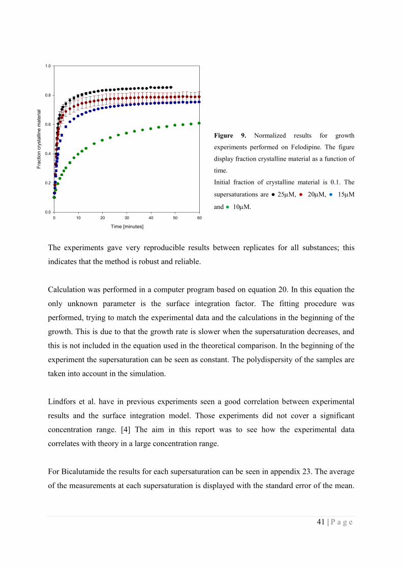
Figure 9. Normalized results for growth
experiments performed on Felodipine. The figure
display fraction crystalline material as a function of
time.
Initial fraction of crystalline material is 0.1. The
supersaturations are ● 25M, ● 20M, ● 15M
and ● 10M.
The experiments gave very reproducible results between replicates for all substances; this
indicates that the method is robust and reliable.
Calculation was performed in a computer program based on equation 20. In this equation the
only unknown parameter is the surface integration factor. The fitting procedure was
performed, trying to match the experimental data and the calculations in the beginning of the
growth. This is due to that the growth rate is slower when the supersaturation decreases, and
this is not included in the equation used in the theoretical comparison. In the beginning of the
experiment the supersaturation can be seen as constant. The polydispersity of the samples are
taken into account in the simulation.
Lindfors et al. have in previous experiments seen a good correlation between experimental
results and the surface integration model. Those experiments did not cover a significant
concentration range. [4] The aim in this report was to see how the experimental data
correlates with theory in a large concentration range.
For Bicalutamide the results for each supersaturation can be seen in appendix 23. The average
of the measurements at each supersaturation is displayed with the standard error of the mean.
Time [minutes]
0 10 20 30 40 50 60
Fra
ctio
n c
rysta
llin
e m
ate
ria
l
0.0
0.2
0.4
0.6
0.8
1.0
42 | P a g e
Time [minutes]
0.0 0.5 1.0 1.5 2.0 2.5 3.0
Fra
ction c
rysta
lline m
ate
rial
0.0
0.2
0.4
0.6
0.8
1.0
=2.5 m
0 20 40 60 80
0.0
0.2
0.4
0.6
0.8
1.0
Time [minutes]
Fra
ction c
rysta
lline m
ate
rial
=30 m
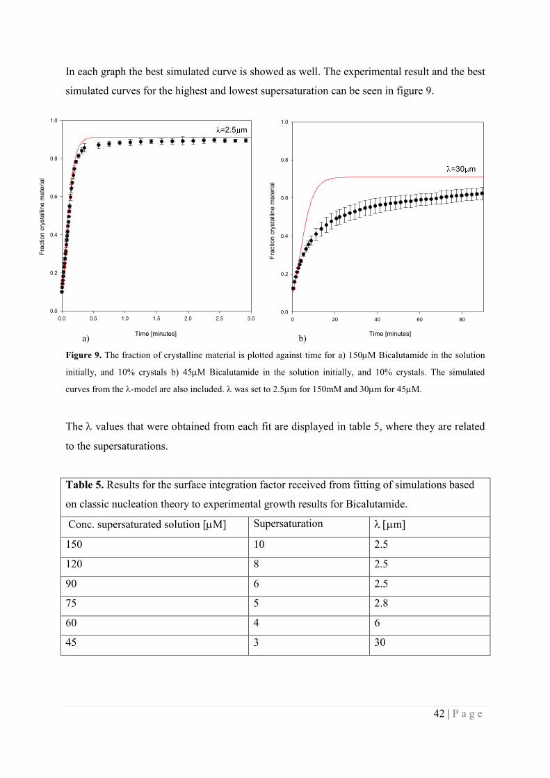
In each graph the best simulated curve is showed as well. The experimental result and the best
simulated curves for the highest and lowest supersaturation can be seen in figure 9.
a) b)
Figure 9. The fraction of crystalline material is plotted against time for a) 150M Bicalutamide in the solution
initially, and 10% crystals b) 45M Bicalutamide in the solution initially, and 10% crystals. The simulated
curves from the -model are also included. was set to 2.5m for 150mM and 30m for 45M.
The values that were obtained from each fit are displayed in table 5, where they are related
to the supersaturations.
Table 5. Results for the surface integration factor received from fitting of simulations based
on classic nucleation theory to experimental growth results for Bicalutamide.
Conc. supersaturated solution [M] Supersaturation m
150 10 2.5
120 8 2.5
90 6 2.5
75 5 2.8
60 4 6
45 3 30
43 | P a g e
The values increases with decreasing supersaturation. This is expected and at concentrations
near the solubility the value approaches infinity. It is expected, but does also show that the
model does not describe crystal growth in a good way. If the agreement had been good, the
theoretical model should be able to describe the growth at all initial concentrations and the
entire growth curves. This is not valid here.
Since the surface integration model seem to work reasonable for high supersaturations, i.e.
the -value is constant, the lowest value that is obtained from the simulations are thus used
in the simulations for the crystal nucleation experiments, where higher supersaturations are
used, see below.
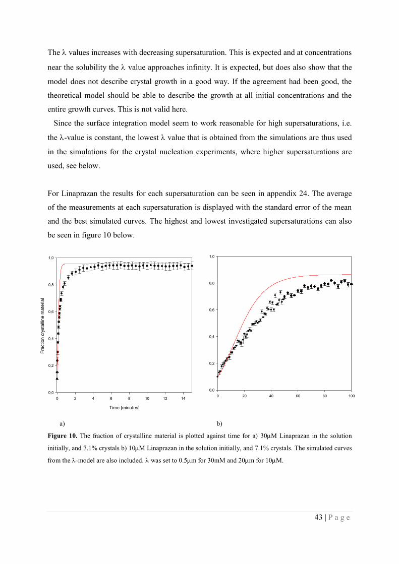
For Linaprazan the results for each supersaturation can be seen in appendix 24. The average
of the measurements at each supersaturation is displayed with the standard error of the mean
and the best simulated curves. The highest and lowest investigated supersaturations can also
be seen in figure 10 below.
a) b)
Figure 10. The fraction of crystalline material is plotted against time for a) 30M Linaprazan in the solution
initially, and 7.1% crystals b) 10M Linaprazan in the solution initially, and 7.1% crystals. The simulated curves
from the -model are also included. was set to 0.5m for 30mM and 20m for 10M.
Time [minutes]
0 2 4 6 8 10 12 14
Fra
ctio
n c
rysta
lline
ma
terial
0,0
0,2
0,4
0,6
0,8
1,0
0 20 40 60 80 100
0,0
0,2
0,4
0,6
0,8
1,0
44 | P a g e
The values that were obtained from each fit are displayed in table 6. The values are quite
stable at high supersaturations, C/S0≥ 5.4. At lower supersaturations the values begin to
increase.
Table 6. Results for the surface integration factor received from fitting of simulations based
on classic nucleation theory to experimental growth results for Linaprazan.
Conc. supersaturated solution [M] Supersaturation m
30 8.1 0.5
25 6.8 0.5
20 5.4 0.6
15 4.1 1.6
10 2.7 20
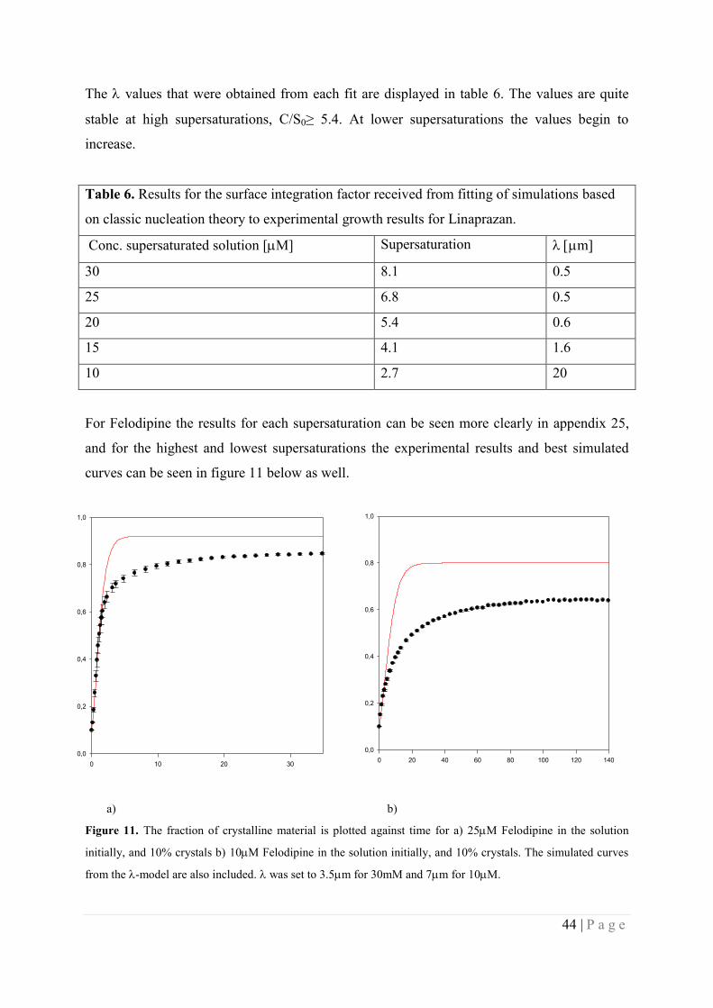
For Felodipine the results for each supersaturation can be seen more clearly in appendix 25,
and for the highest and lowest supersaturations the experimental results and best simulated
curves can be seen in figure 11 below as well.
a) b)
Figure 11. The fraction of crystalline material is plotted against time for a) 25M Felodipine in the solution
initially, and 10% crystals b) 10M Felodipine in the solution initially, and 10% crystals. The simulated curves
from the -model are also included. was set to 3.5m for 30mM and 7m for 10M.
0 10 20 30
0,0
0,2
0,4
0,6
0,8
1,0
0 20 40 60 80 100 120 140
0,0
0,2
0,4
0,6
0,8
1,0

45 | P a g e
The values that were obtained from each fit are displayed in table 7. The results deviate
some and do not show a significant increase in l at the lowest supersaturation. This might
however be due not investigating at as low supersaturations as for the other two substances.
Table 7. Results for the surface integration factor received from fitting of simulations based
on classic nucleation theory to experimental growth results for Felodipine.
Conc. supersaturated solution [M] Supersaturation m
25 10 3.5
20 8 2.8
15 6 3.0
10 4 7
The trend, that the values are low at the highest supersaturation and increases with lower
supersaturation, can be seen for all three substances. This indicates that there is a barrier for
crystal growth, the same way as for crystal nucleation. This does in turn indicate that growth
as well might be a nucleation based process. Here the nucleation would be two dimensional
surface nucleation. For nucleation the barrier decreases with increasing supersaturation, and
this would for crystal growth be related to the faster rate at higher supersaturations.
The-model can describe dissolution properly, but not growth. This might be due to that
when a crystal dissolves; the shape goes from a characteristic, for example cubic to more and
more spherical. This indicates that the dissolution will be a faster process that is diffusion
controlled. The growth on the other hand, has a more complex mechanism. [29]
Due to the poor agreement with the -model, comparison between experimental results and
polynuclear surface nucleation theory as described by Hillig and Nielsen has also been done.
This comparison gives a frequency in and an interfacial tension, 3D, see equation 30. The
frequency is thought to reflect the incorporation of monomer and the sl is the apparent three
dimensional interfacial tension for crystal growth.
46 | P a g e
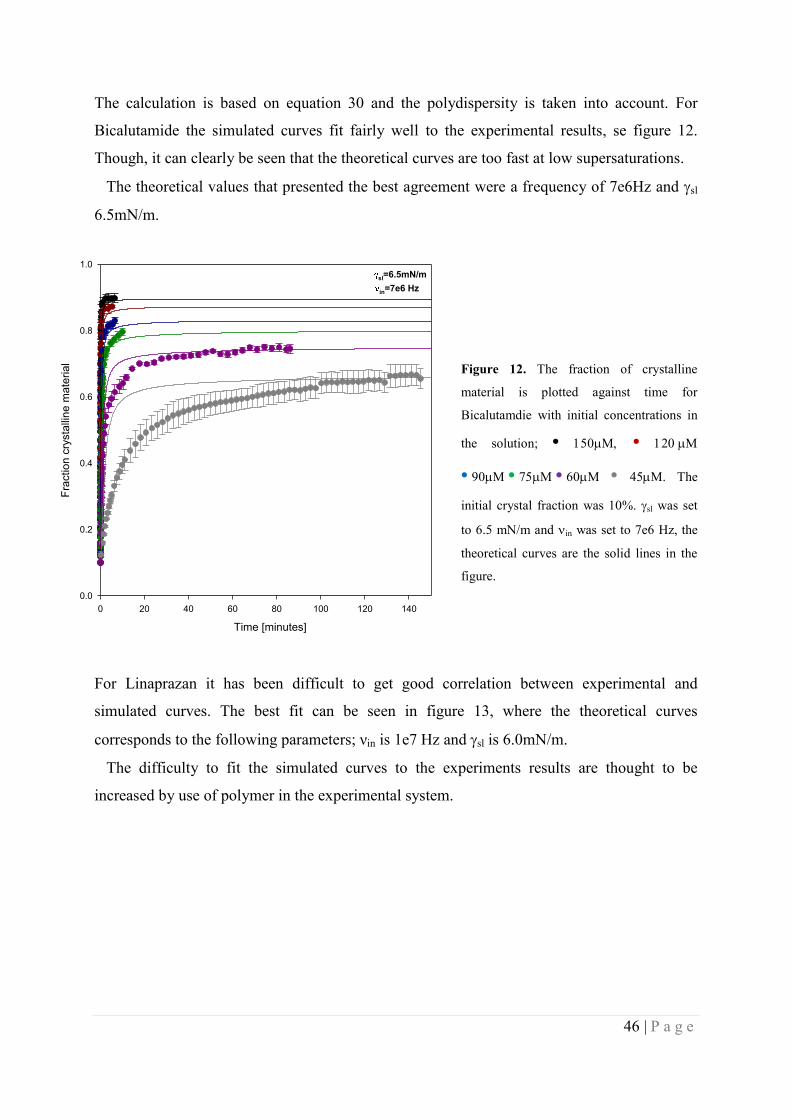
The calculation is based on equation 30 and the polydispersity is taken into account. For
Bicalutamide the simulated curves fit fairly well to the experimental results, se figure 12.
Though, it can clearly be seen that the theoretical curves are too fast at low supersaturations.
The theoretical values that presented the best agreement were a frequency of 7e6Hz and sl
6.5mN/m.
Figure 12. The fraction of crystalline
material is plotted against time for
Bicalutamdie with initial concentrations in
the solution; • •
•••M • 45M. The
initial crystal fraction was 10%. sl was set
to 6.5 mN/m and in was set to 7e6 Hz, the
theoretical curves are the solid lines in the
figure.
For Linaprazan it has been difficult to get good correlation between experimental and
simulated curves. The best fit can be seen in figure 13, where the theoretical curves
corresponds to the following parameters; νin is 1e7 Hz and sl is 6.0mN/m.
The difficulty to fit the simulated curves to the experiments results are thought to be
increased by use of polymer in the experimental system.
Time [minutes]
0 20 40 60 80 100 120 140
Fra
ctio
n c
rysta
llin
e m
ate
ria
l
0.0
0.2
0.4
0.6
0.8
1.0
sl=6.5mN/m
in=7e6 Hz

47 | P a g e
Figure 13. The fraction of crystalline material
is plotted against time for Linaprazan with
initial concentrations in the solution; •
• •••M. The
initial crystal fraction was 7.1%. sl was set to
6.0 mN/m and in was set to 1e7 Hz, the
theoretical curves are the solid lines in the
figure.
For Felodipine the calculated results and the experimental data agree very well. This is very
encouraging and is hopefully and indication that 2D nucleation is the right track regarding
crystal growth theories.
The fit between experimental data and simulated curves can be seen in figure 14, νin is 6e7
Hz and sl is 10.4 mN/m.
Figure 14. The fraction of crystalline
material is plotted against time for Felodipine
with initial concentrations in the solution;
• • ••. The
initial crystal fraction was 10%. sl was set to
10.4mN/m and in was set to 6e7 Hz, the
theoretical curves are the solid lines in the
figure.
Time [minutes]
0 20 40 60 80 100 120 140
Fra
ctio
n c
rysta
llin
e m
ate
ria
l
0.0
0.2
0.4
0.6
0.8
1.0
sl=10.4mN/m
in=6e7 Hz
Time [minutes]
0 20 40 60 80 100
Fra
ctio
n c
rysta
llin
e m
ate
ria
l
0.0
0.2
0.4
0.6
0.8
1.0
sl=6.0mN/m
in=1e7 Hz

48 | P a g e
To summarize the results above, nanocrystal growth for Felodpine can be described nicely by
the Hillig-Nielsen theory, Bicalutamide and Linaprazan does however not coincide entirely
with theoretical calculations.
It can be seen that the simulated curves cannot describe all supersaturations with the same
values of sl and in. This might be due to this model being based on poly nuclear growth. This
mechanism is thought to be true for high supersaturations, but probably is not valid at low
supersaturations. The Hillig-Nielsen model will thus give theoretical curves that go to fast at
low supersaturations.
It can however be seen that the model is better, and also that it takes into consideration the
decrease in concentration of the supersaturated solution. The simulated curves do not continue
to solubility, it continues to the metastable zone for growth. This should when the parameters
are set properly also coincide with the experimentally received values.
Due to the observations above, that the Hillig-Nielsen model works well at high
supersaturations, but is too fast at low supersaturations, might indicate a different mechanism
depending on the supersaturation. The theoretical Obretenov interpolation model, which
combines both poly and mono nuclear growth was used in calculations. The results for all
substances and supersaturations are to be seen below. The Obretenov interpolation model can
be simulated by equation 35 and the polydispersity is taken into account.
For Bicalutamide sl was determined to 4mN/m and υin was determined to 1e6 Hz. The curves
do coincide fairly well, se figure 15. It can be seen that the model can describe the growth at
high supersaturations in a much better way than at low ones. It can also be seen that the
agreement is better here, than for the Hillig-Nielsen model.
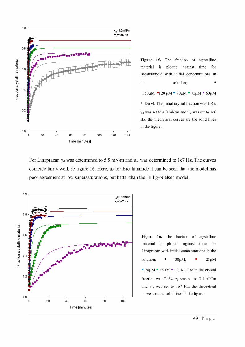
49 | P a g e
Figure 15. The fraction of crystalline
material is plotted against time for
Bicalutamdie with initial concentrations in
the solution; •
••••M
• 45M. The initial crystal fraction was 10%.
sl was set to 4.0 mN/m and in was set to 1e6
Hz, the theoretical curves are the solid lines
in the figure.
For Linaprazan sl was determined to 5.5 mN/m and υin was determined to 1e7 Hz. The curves
coincide fairly well, se figure 16. Here, as for Bicalutamide it can be seen that the model has
poor agreement at low supersaturations, but better than the Hillig-Nielsen model.
Figure 16. The fraction of crystalline
material is plotted against time for
Linaprazan with initial concentrations in the
solution; • •
•••M. The initial crystal
fraction was 7.1%. sl was set to 5.5 mN/m
and in was set to 1e7 Hz, the theoretical
curves are the solid lines in the figure.
Time [minutes]
0 20 40 60 80 100 120 140
Fra
ctio
n c
rysta
llin
e m
ate
ria
l
0.0
0.2
0.4
0.6
0.8
1.0
sl=4.0mN/m
in=1e6 Hz
Time [minutes]
0 20 40 60 80 100
Fra
ctio
n c
rysta
llin
e m
ate
ria
l
0.0
0.2
0.4
0.6
0.8
1.0
sl=5.5mN/m
in=1e7 Hz
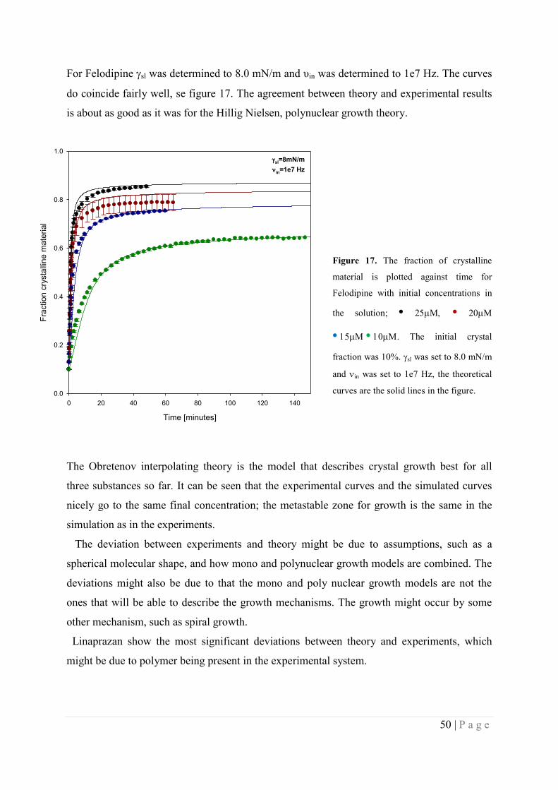
50 | P a g e
For Felodipine sl was determined to 8.0 mN/m and υin was determined to 1e7 Hz. The curves
do coincide fairly well, se figure 17. The agreement between theory and experimental results
is about as good as it was for the Hillig Nielsen, polynuclear growth theory.
Figure 17. The fraction of crystalline
material is plotted against time for
Felodipine with initial concentrations in
the solution; • •
••. The initial crystal
fraction was 10%. sl was set to 8.0 mN/m
and in was set to 1e7 Hz, the theoretical
curves are the solid lines in the figure.
The Obretenov interpolating theory is the model that describes crystal growth best for all
three substances so far. It can be seen that the experimental curves and the simulated curves
nicely go to the same final concentration; the metastable zone for growth is the same in the
simulation as in the experiments.
The deviation between experiments and theory might be due to assumptions, such as a
spherical molecular shape, and how mono and polynuclear growth models are combined. The
deviations might also be due to that the mono and poly nuclear growth models are not the
ones that will be able to describe the growth mechanisms. The growth might occur by some
other mechanism, such as spiral growth.
Linaprazan show the most significant deviations between theory and experiments, which
might be due to polymer being present in the experimental system.
Time [minutes]
0 20 40 60 80 100 120 140
Fra
ctio
n c
rysta
llin
e m
ate
ria
l
0.0
0.2
0.4
0.6
0.8
1.0
sl=8mN/m
in=1e7 Hz
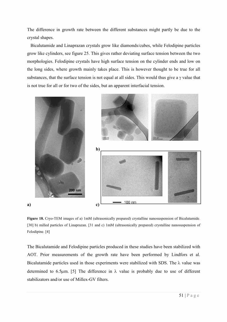
51 | P a g e
The difference in growth rate between the different substances might partly be due to the
crystal shapes.
Bicalutamide and Linaprazan crystals grow like diamonds/cubes, while Felodipine particles
grow like cylinders, see figure 25. This gives rather deviating surface tension between the two
morphologies. Felodipine crystals have high surface tension on the cylinder ends and low on
the long sides, where growth mainly takes place. This is however thought to be true for all
substances, that the surface tension is not equal at all sides. This would thus give a value that
is not true for all or for two of the sides, but an apparent interfacial tension.
b)
a) c)
Figure 18. Cryo-TEM images of a) 1mM (ultrasonically prepared) crystalline nanosuspension of Bicalutamide.
[30] b) milled particles of Linaprazan. [31 and c) 1mM (ultrasonically prepared) crystalline nanosuspension of
Felodipine. [4]
The Bicalutamide and Felodipine particles produced in these studies have been stabilized with
AOT. Prior measurements of the growth rate have been performed by Lindfors et al.
Bicalutamide particles used in those experiments were stabilized with SDS. The value was
determined to 6.5m. [5] The difference in value is probably due to use of different
stabilizators and/or use of Millex-GV filters.

52 | P a g e
For Felodipine previous growth experiments have been performed by Lindfors et al. The
value was 2.5m for particles ultrasonically prepared with 0.2% (w/w) PVP and 0.25mM
SDS as stabilization. [4] The value determined in this study was 3m. The difference here is
probably due to different stabilization. Previously, Felodipine particles have been milled as
well, with PVP/AOT, this gave = 4m. The difference between these experiments also
indicates that the stabilization affects the growth rate to some extent.
For Linaprazan prior measurements have been performed by Lindfors et al. on milled
particles that were stabilized with 1.33 % (w/w) PVP (K30) and 0.067 % (w/w) AOT. The
value for these particles was determined to 2m. [32] The same has been done here, due to
problems when trying to perform the experiments on ultrasonically prepared particles. From
the performed experiments the value was determined to 0.5m. The difference is probably
due to use of different filters.
Interesting experimental observations were made during growth experiments on Linaprazan.
When at the end of an experiment, the final intensity should be measured; the vessel was
turned gently once. The turn resulted in lower intensity then before. If the procedure was
repeated and the more violent the turning was made, the lower the final intensity was.
This result might be an indication that the growing dendrites that falls of easily when the
vessel is turned.
The particles used in these studies showed rather different stabilities. For example
Bicalutamide particles were stable for several weeks while Felodipine was only stable for 2
days.
The growth rate for Bicalutamide was significantly faster compared to results presented by
Lindfors et al [5]. The value determined in that paper was 6.5 m compared to 2.5 in this
studie. This is partly due to the filtration performed by Lindfors et al was performed with
Millex-GV filters.
4.4.5. Growth experiments with different amount of stabilization
Growth experiments with different stabilization were performed the same way as the growth
experiments above. The experiments were performed to see how the stabilization affects the
growth rate.
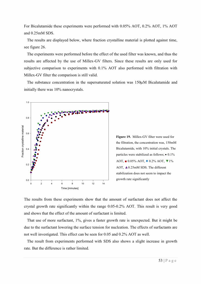
53 | P a g e
For Bicalutamide these experiments were performed with 0.05% AOT, 0.2% AOT, 1% AOT
and 0.25mM SDS.
The results are displayed below, where fraction crystalline material is plotted against time,
see figure 26.
The experiments were performed before the effect of the used filter was known, and thus the
results are affected by the use of Millex-GV filters. Since these results are only used for
subjective comparison to experiments with 0.1% AOT also performed with filtration with
Millex-GV filter the comparison is still valid.
The substance concentration in the supersaturated solution was 150M Bicalutamide and
initially there was 10% nanocrystals.
Figure 19. Millex-GV filter were used for
the filtration, the concentration was, 150mM
Bicalutamide, with 10% initial crystals. The
particles were stabilized as follows; 0.1%
AOT, ■ 0.05% AOT, ♦ 0.2% AOT, ▼1%
AOT, ▲0.25mM SDS. The different
stabilization does not seem to impact the
growth rate significantly
The results from these experiments show that the amount of surfactant does not affect the
crystal growth rate significantly within the range 0.05-0.2% AOT. This result is very good
and shows that the effect of the amount of surfactant is limited.
That use of more surfactant, 1%, gives a faster growth rate is unexpected. But it might be
due to the surfactant lowering the surface tension for nucleation. The effects of surfactants are
not well investigated. This effect can be seen for 0.05 and 0.2% AOT as well.
The result from experiments performed with SDS also shows a slight increase in growth
rate. But the difference is rather limited.
Time [minutes]
0 2 4 6 8 10 12 14
Fra
ctio
n c
rysta
llin
e m
ate
ria
l
0.0
0.2
0.4
0.6
0.8
1.0
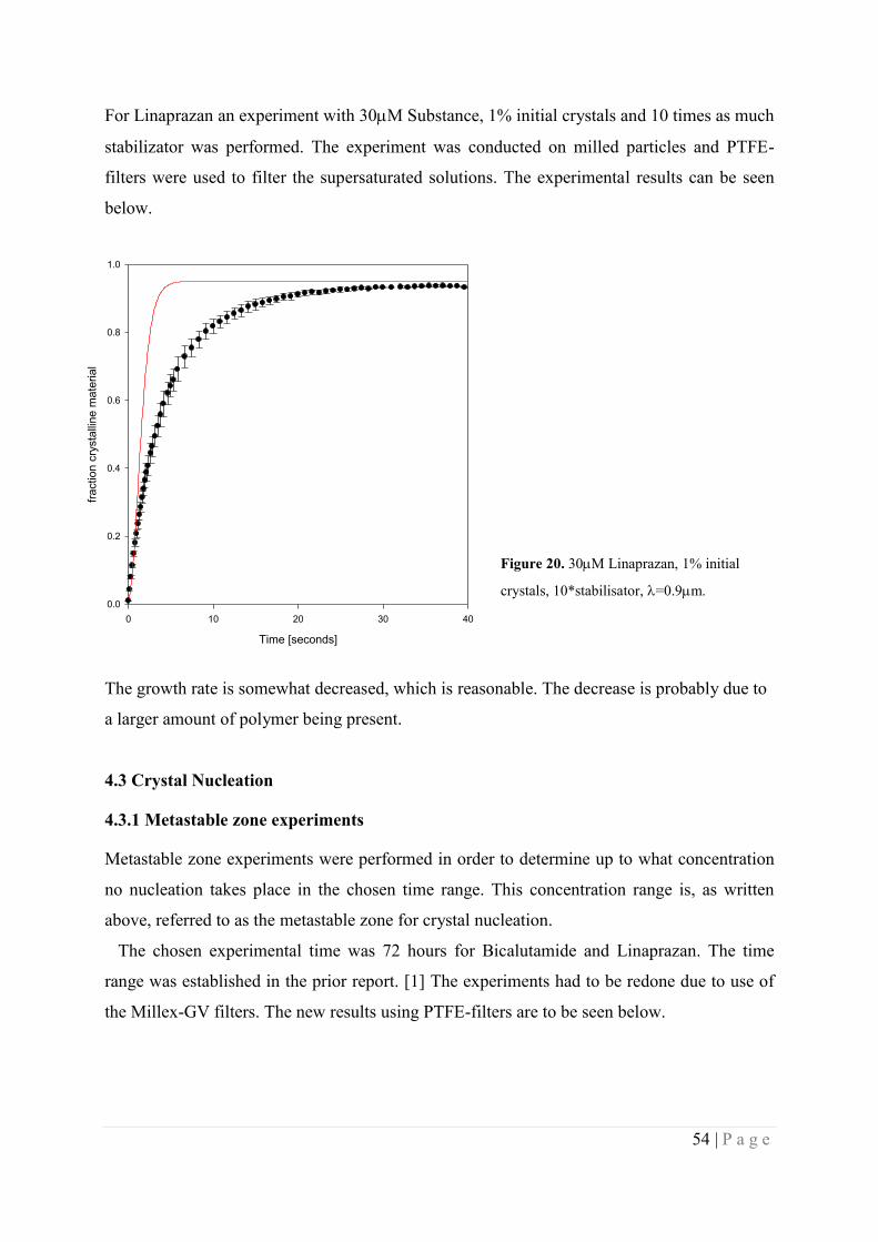
54 | P a g e
For Linaprazan an experiment with 30M Substance, 1% initial crystals and 10 times as much
stabilizator was performed. The experiment was conducted on milled particles and PTFE-
filters were used to filter the supersaturated solutions. The experimental results can be seen
below.
Figure 20. 30M Linaprazan, 1% initial
crystals, 10*stabilisator, =0.9m.
The growth rate is somewhat decreased, which is reasonable. The decrease is probably due to
a larger amount of polymer being present.
4.3 Crystal Nucleation
4.3.1 Metastable zone experiments
Metastable zone experiments were performed in order to determine up to what concentration
no nucleation takes place in the chosen time range. This concentration range is, as written
above, referred to as the metastable zone for crystal nucleation.
The chosen experimental time was 72 hours for Bicalutamide and Linaprazan. The time
range was established in the prior report. [1] The experiments had to be redone due to use of
the Millex-GV filters. The new results using PTFE-filters are to be seen below.
Time [seconds]
0 10 20 30 40
fraction c
rysta
lline m
ate
rial
0.0
0.2
0.4
0.6
0.8
1.0

55 | P a g e
Figure 21. Result for metastable zone
experiments for Bicalutamide, the
concentration after 72 hours (the nucleation
time) is plotted against the initial
concentration. The final concentrations have
been compensated for loss by filtration. The
solid line is a guide to the eye. Different
symbols indicate different occasions.
The metastable zone reaches up to about 220M for 72 hours. It can also be seen in the figure
that above 200M there are almost no symbols in the middle region. All samples, but few,
have either the same concentration as initially or a low concentration, about 25M. This
“birfucation” might indicate that the crystallization process for Bicalutamide is affected by
secondary nucleation.
If the primary nucleation takes place, secondary nucleation follows and rapidly gives a large
amount of crystals. This phenomenon is not well understood theoretically, but might be due to
existing nuclei stabilizing the formation of new nuclei, or that pieces of larger crystals falls of
giving new nuclei that can continue to grow. What is known is however that secondary
nucleation can exist and that it gives a cascade reaction in terms of amount of crystals.
For Linaprazan the metastable zone reaches up to slightly above 20M with initial filtration.
At higher concentrations the amount after 72 hours is lower than the initial, see figure 22.
Initial concentration [M]
0 100 200 300 400 500
Co
nce
ntr
atio
n a
fte
r 7
2 h
ou
rs [
M]
0
100
200
300
400
500
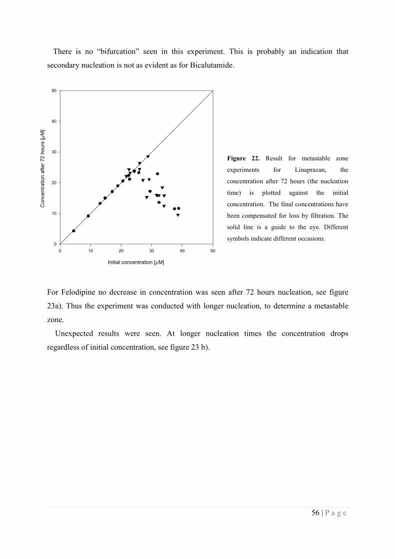
56 | P a g e
There is no “bifurcation” seen in this experiment. This is probably an indication that
secondary nucleation is not as evident as for Bicalutamide.
Figure 22. Result for metastable zone
experiments for Linaprazan, the
concentration after 72 hours (the nucleation
time) is plotted against the initial
concentration. The final concentrations have
been compensated for loss by filtration. The
solid line is a guide to the eye. Different
symbols indicate different occasions.
For Felodipine no decrease in concentration was seen after 72 hours nucleation, see figure
23a). Thus the experiment was conducted with longer nucleation, to determine a metastable
zone.
Unexpected results were seen. At longer nucleation times the concentration drops
regardless of initial concentration, see figure 23 b).
0 10 20 30 40 50
0
10
20
30
40
50
Initial concentration [M]
Co
nce
ntr
atio
n a
fte
r 7
2 h
ou
rs [
M]
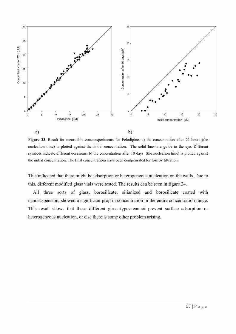
57 | P a g e
a) b)
Figure 23. Result for metastable zone experiments for Felodipine. a) the concentration after 72 hours (the
nucleation time) is plotted against the initial concentration. The solid line is a guide to the eye. Different
symbols indicate different occasions. b) the concentration after 10 days (the nucleation time) is plotted against
the initial concentration. The final concentrations have been compensated for loss by filtration.
This indicated that there might be adsorption or heterogeneous nucleation on the walls. Due to
this, different modified glass vials were tested. The results can be seen in figure 24.
All three sorts of glass, borosilicate, silianized and borosilicate coated with
nanosuspension, showed a significant prop in concentration in the entire concentration range.
This result shows that these different glass types cannot prevent surface adsorption or
heterogeneous nucleation, or else there is some other problem arising.
0 5 10 15 20 25 30
0
5
10
15
20
25
30
Initial conc. [uM]
Concentr
ation a
fter
72 h
[uM
]
0 5 10 15 20 25
0
5
10
15
20
25
Initial concentration [M]C
oncentr
ation a
fter
10 d
ays [M
]

58 | P a g e
Figure 24. Result for metastable zone
experiments for Felodipine performed in different
glass vials. ● represents ordinary borosilicate
vials, ▲ vials coated with nanosuspension and ♦,
silanized vials. The final concentrations have
been compensated for loss by filtration.
It was thought that there might be something that affects the samples when they are standing
on the anti-vibration table, and thus experiments were conducted simultaneously on the anti-
vibration table and an ordinary table, both situated in the same room. The experiment were
performed in ordinary glass vials, and the loss was for some reason not as significant as
before, but still there is some loss and no clear drop, see figure 25 below.
Figure 25. Result for metastable zone
experiments for Felodipine performed on
different tables. ● represents samples that
nucleated on the anti-vibration table, ■ are
samples that nucleated on the ordinary table.
The final concentrations have been
compensated for loss by filtration.
0 5 10 15 20 25 30
0
5
10
15
20
25
30
Initial concentration [M]
Concnentr
ation a
fter
10 d
ays [
]
Initial concentration after filtration [M]
0 5 10 15 20 25 30
Concentr
ation a
fter
14 d
ays [M
]
0
5
10
15
20
25
30
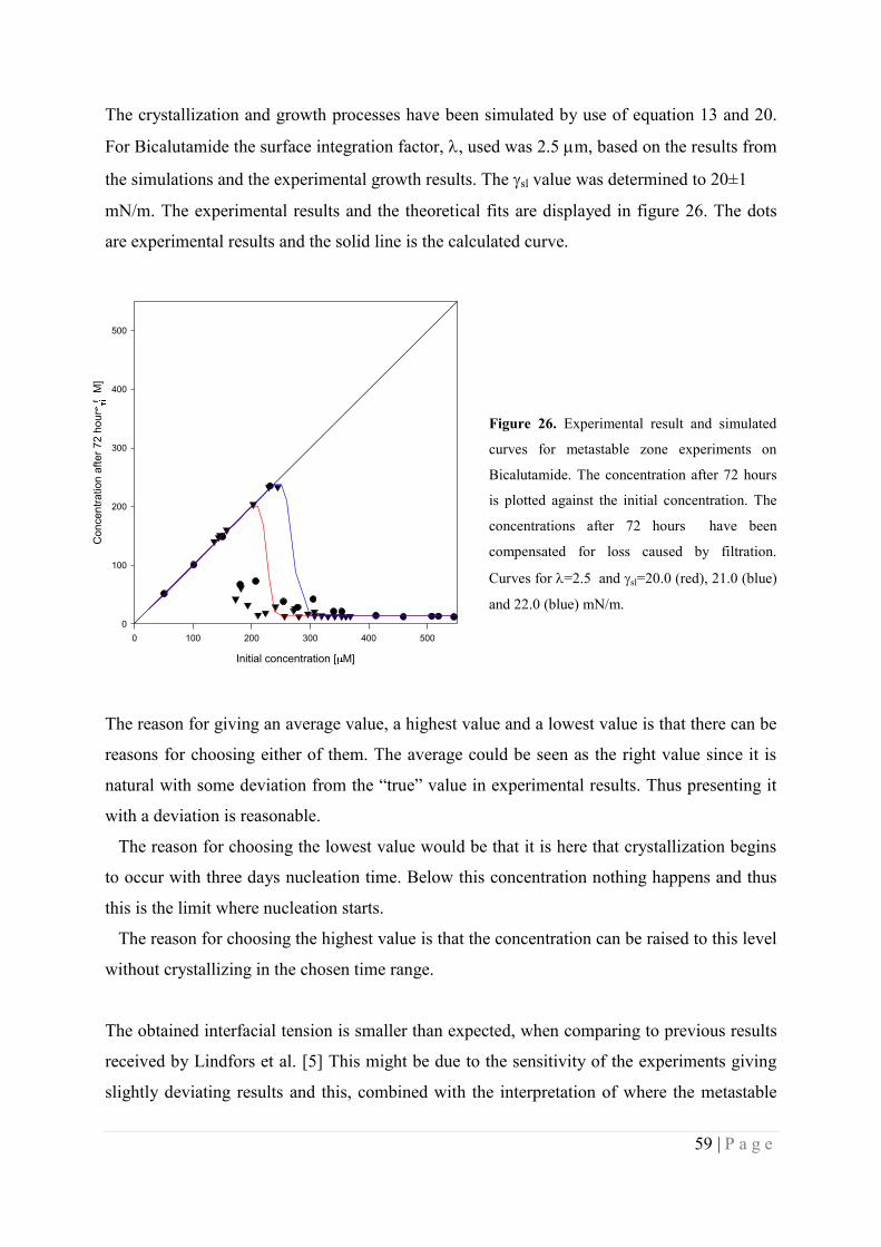
59 | P a g e
The crystallization and growth processes have been simulated by use of equation 13 and 20.
For Bicalutamide the surface integration factor, , used was 2.5 m, based on the results from
the simulations and the experimental growth results. The sl value was determined to 20±1
mN/m. The experimental results and the theoretical fits are displayed in figure 26. The dots
are experimental results and the solid line is the calculated curve.
Figure 26. Experimental result and simulated
curves for metastable zone experiments on
Bicalutamide. The concentration after 72 hours
is plotted against the initial concentration. The
concentrations after 72 hours have been
compensated for loss caused by filtration.
Curves for =2.5 and sl=20.0 (red), 21.0 (blue)
and 22.0 (blue) mN/m.
The reason for giving an average value, a highest value and a lowest value is that there can be
reasons for choosing either of them. The average could be seen as the right value since it is
natural with some deviation from the “true” value in experimental results. Thus presenting it
with a deviation is reasonable.
The reason for choosing the lowest value would be that it is here that crystallization begins
to occur with three days nucleation time. Below this concentration nothing happens and thus
this is the limit where nucleation starts.
The reason for choosing the highest value is that the concentration can be raised to this level
without crystallizing in the chosen time range.
The obtained interfacial tension is smaller than expected, when comparing to previous results
received by Lindfors et al. [5] This might be due to the sensitivity of the experiments giving
slightly deviating results and this, combined with the interpretation of where the metastable
Initial concentration [ M]
0 100 200 300 400 500
Co
nce
ntr
atio
n a
fte
r 7
2 h
ou
rs [
M]
0
100
200
300
400
500
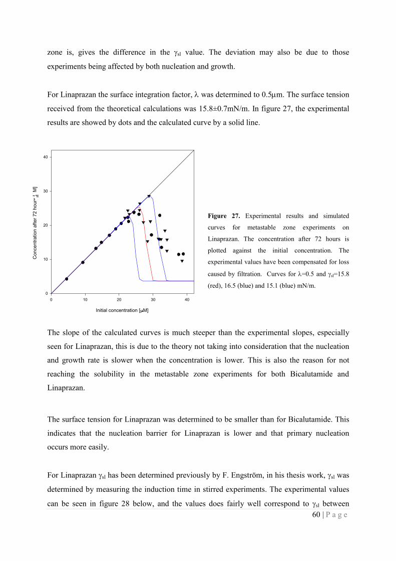
60 | P a g e
zone is, gives the difference in the sl value. The deviation may also be due to those
experiments being affected by both nucleation and growth.
For Linaprazan the surface integration factor, was determined to 0.5m. The surface tension
received from the theoretical calculations was 15.8±0.7mN/m. In figure 27, the experimental
results are showed by dots and the calculated curve by a solid line.
Figure 27. Experimental results and simulated
curves for metastable zone experiments on
Linaprazan. The concentration after 72 hours is
plotted against the initial concentration. The
experimental values have been compensated for loss
caused by filtration. Curves for =0.5 and sl=15.8
(red), 16.5 (blue) and 15.1 (blue) mN/m.
The slope of the calculated curves is much steeper than the experimental slopes, especially
seen for Linaprazan, this is due to the theory not taking into consideration that the nucleation
and growth rate is slower when the concentration is lower. This is also the reason for not
reaching the solubility in the metastable zone experiments for both Bicalutamide and
Linaprazan.
The surface tension for Linaprazan was determined to be smaller than for Bicalutamide. This
indicates that the nucleation barrier for Linaprazan is lower and that primary nucleation
occurs more easily.
For Linaprazan sl has been determined previously by F. Engström, in his thesis work, sl was
determined by measuring the induction time in stirred experiments. The experimental values
can be seen in figure 28 below, and the values does fairly well correspond to sl between
0 10 20 30 40
0
10
20
30
40
Initial concentration [ M]
Co
nce
ntr
atio
n a
fte
r 7
2 h
ou
rs [
M]

61 | P a g e
15.7mN/m and 16.0mN/m, compared to 15.8mN/m in this report. The values of the surface
tension has been received by using =0.5m, as found in this report.
These values are very similar and do thus indicated that the value is in the correct region.
Figure 28. Experimental values for the
induction time for Linaprazan are plotted in
the figure. The dotted lines are theoretical
curves, corresponding to ····· =0.5mm
and sl=15.7mN/m and ····· =0.5mm and
sl=16.0 mN/m.
For Felodipine the correct metastable zone has been difficult to determine. There has been
substantial substance loss in the experiments, regardless of which method was used to
eliminate large particles in the beginning of the experiment. The loss was difficult to get an
understanding of. The main problem is most likely due to surface adsorption and/or
heterogeneous nucleation. It was however surprising that change of glass vessels did not
impact the results in a positive direction. The silanized vials were thought to minimize
interactions, but no change was seen in the results.
Since no well established metastable zone has been determined, the sl value is instead
presented as a “lowest value”. The metastable zone seems to reach higher than what can be
detected in the experiments and the values presented below are thus detecting the limit where
no nucleation has begun in the chosen time range.
16 (Vm/N
A)2 / [3(kT)
3ln
2(C/S
0)]
8.0e+6 9.0e+6 1.0e+7 1.1e+7 1.2e+7 1.3e+7 1.4e+7
t ind
(s)
1
10
100
1000
10000
30µM
40µM
sl=16.0 mN/m
=0.5 m
sl=15.7 mN/m
=0.5 m

62 | P a g e
The result below presents both 72 hours nucleation time, figure 29 a) and 14 days
nucleation time, figure 29 b).
a) b)
Figure 29. Experimental results and simulated curves for metastable zone experiments on felodipine. The
concentration after the nucleation time is plotted against the initial concentration. The experimental values have
been compensated for loss caused by filtration. a) nucleation time=72 hours, = 2.8m gave sl=18.5mN/m, b)
nucleation time=14days, = 2.8m gave sl=18.0mN/m.
The values differ slightly, but when looking at the experimental results it can be seen that the
experiment that has been conducted for 14 days have more deviation from the expected line.
These results are thus more uncertain. It is easier to evaluate the results from the experiment
that has been conducted for 72 hours. It can thus be concluded that the sl value for Felodipine
is at the lowest 18.5mN/m.
4.3.3 Crystal nucleation experiments
Crystal nucleation experiments have been performed on Bicalutamide for one nucleation
concentration, 440M. The experiments have been performed according to the procedure in
section 3.11.7 and evaluated according to section 3.11.8.
The nucleation times ranged from zero minutes (metastable zone) to one hour and fifteen
minutes. The concentration during the growth was 175M, which is within the determined
0 5 10 15 20 25 30
0
5
10
15
20
25
30
Initial conc. [uM]
Concentr
ation a
fter
72 h
[uM
]
Initial concentration [m]
0 5 10 15 20 25 30
Concentr
ation a
fter
14 d
ays [m
]
0
5
10
15
20
25
30
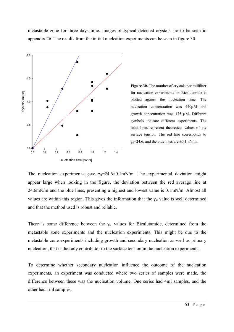
63 | P a g e
metastable zone for three days time. Images of typical detected crystals are to be seen in
appendix 26. The results from the initial nucleation experiments can be seen in figure 30.
Figure 30. The number of crystals per milliliter
for nucleation experiments on Bicalutamide is
plotted against the nucleation time. The
nucleation concentration was 440M and
growth concentration was 175 M. Different
symbols indicate different experiments. The
solid lines represent theoretical values of the
surface tension. The red line corresponds to
sl=24.6, and the blue lines are ±0.1mN/m.
The nucleation experiments gave sl=24.6±0.1mN/m. The experimental deviation might
appear large when looking in the figure, the deviation between the red average line at
24.6mN/m and the blue lines, presenting a highest and lowest value is 0.1mN/m. Almost all
values are within this region. This gives the information that the sl value is well determined
and that the method used is robust and reliable.
There is some difference between the sl values for Bicalutamide, determined from the
metastable zone experiments and the nucleation experiments. This might be due to the
metastable zone experiments including growth and secondary nucleation as well as primary
nucleation, that is the only contributor to the surface tension in the nucleation experiments.
To determine whether secondary nucleation influence the outcome of the nucleation
experiments, an experiment was conducted where two series of samples were made, the
difference between these was the nucleation volume. One series had 4ml samples, and the
other had 1ml samples.
nucteation time [hours]
0.0 0.2 0.4 0.6 0.8 1.0 1.2 1.4
cry
sta
ls/
ml [s
t]
0.0
0.5
1.0
1.5
2.0
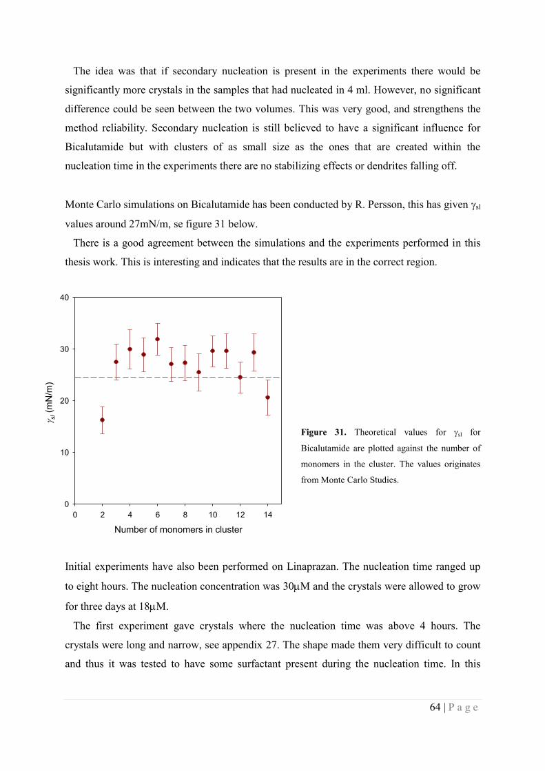
64 | P a g e
The idea was that if secondary nucleation is present in the experiments there would be
significantly more crystals in the samples that had nucleated in 4 ml. However, no significant
difference could be seen between the two volumes. This was very good, and strengthens the
method reliability. Secondary nucleation is still believed to have a significant influence for
Bicalutamide but with clusters of as small size as the ones that are created within the
nucleation time in the experiments there are no stabilizing effects or dendrites falling off.
Monte Carlo simulations on Bicalutamide has been conducted by R. Persson, this has given sl
values around 27mN/m, se figure 31 below.
There is a good agreement between the simulations and the experiments performed in this
thesis work. This is interesting and indicates that the results are in the correct region.
Figure 31. Theoretical values for sl for
Bicalutamide are plotted against the number of
monomers in the cluster. The values originates
from Monte Carlo Studies.
Initial experiments have also been performed on Linaprazan. The nucleation time ranged up
to eight hours. The nucleation concentration was 30M and the crystals were allowed to grow
for three days at 18M.
The first experiment gave crystals where the nucleation time was above 4 hours. The
crystals were long and narrow, see appendix 27. The shape made them very difficult to count
and thus it was tested to have some surfactant present during the nucleation time. In this
Number of monomers in cluster
0 2 4 6 8 10 12 14
sl (
mN
/m)
0
10
20
30
40
65 | P a g e
experiment no crystals were seen and thus the initial experiment was repeated, this time no
crystals were to be seen.
These initial experiments have only given the information that Linaprazan crystals can be
detected.
The new nucleation method presented above, with its initial results is believed to be a good
method.
The experiments are fairly easy to perform. The results seem to be reliable and robust. The
method does also present many opportunities to perform these experiments with some
modifications to receive a lot of new information. The experimental setup can be used with
different additives in the supersaturated solutions, to see how nucleation is affected. It is also
possible to introduce a single crystal into the solution at t=0, to see how this affects the
crystallization rate, i.e. the effect of secondary nucleation.

66 | P a g e
5. Conclusions
Experimental method development has been an important part of this thesis work. The result
is several experimental setups that feel reliable and very informative.
The crystal nucleation experimental setup seems reliable and the experiment is relatively
easy to perform. From this experiment the surface tension can be determined.
The growth and dissolution experiments give concurring results between different
experiments and do thus seem reliable. These experiments give information about the surface
integration kinetics.
The metastable zone experiments gave valuable information about the limit of nucleation
for a certain time and thus the surface tension.
The surface tension was determined to 20±1mN/m for Bicalutamide from the metastable zone
experiments. From the nucleation experiments the value was determined to 24.6±0.1mN/m.
These values do not agree and this might be due to secondary nucleation.
Nucleation of Bicalutamide seems to be largely influenced by secondary nucleation. This is
seen in the metastable zone experiments where a bifurcation clearly is seen. It has however
successfully been determined that secondary nucleation is not present when the crystals are
very small. This has given a solid base for the crystal nucleation experiments that has been
carried out.
Agreement between the nucleation results and performed Monte Carlo simulations do also
indicate that the results are reliable.
The surface tension for Linaprazan was determined to 15.8±0.7 mN/m. This indicates that the
barrier for nucleation is slightly lower for Linaprazan than for Bicalutamide.
Felodipine results indicate a barrier for nucleation that is above 18.5mN/m. The true value has
been very difficult to find. The reason for this is partially due to the low amorphous solubility.
This makes it difficult to make solutions of high supersaturation.
67 | P a g e
The growth experiments have given significantly lower values in this thesis work than in the
prior. This is thought to mainly be due to working with more unaffected systems and avoiding
Millex GV-filters.
The understanding of the filters large impact on the nucleation related processes was an
important finding in this report.
The values that have been determined are 2.5m for Bicalutamide, 0.5m for Linaprazan
and 2.8m for Felodipine. The surface integration model is not able to describe growth in a
satisfactory way, especially not at low supersaturations.
The Hillig Nielsen, polynuclear model, had better agreement, and gave sl 6.5 mN/m and
7*106 Hz for Bicalutamide. For Linaprazan the corresponding values were 6.0 mN/m and
1*107 Hz. For Felodipine the frequency was 6*10
7 Hz and the surface tension was 10.4mN/m.
The model was able to describe all growth curves well for Felodipine and fairly well for
Linaprazan and Bicalutamide.
The Obretenov interpolation model, where both mono- and polynuclear growth are included
gave sl 4.0mN/m and 1*106 Hz for Bicalutamide. For Linaprazan the corresponding values
were 5.5 mN/m and 1*107 Hz. For Felodipine the frequency was 1*10
7 Hz and the surface
tension was 8.0mN/m. The Obretenov interpolation model was the best at describing all
growth curves well for all substances.
The difference between the three substances might be due to different shapes of the crystals
when growing.
It was very interesting to find that within reasonable limits, the growth is unaffected by the
amount of stabilizator and only slightly affected by the type used.
The crystal dissolution experiments have showed that the process is diffusion controlled. This
is probably due to no shape maintenance during the dissolution.

68 | P a g e
6. Future Work
More crystal nucleation experiments need to be performed, primarily on more substances and
also on different nucleation concentrations for each of these substances.
Further, secondary nucleation experiments are an interesting extension that would be
possible to continue with. A crystal would then be added to the supersaturated solution at t=0,
and removed at t=tnuc, and the solution would then be diluted into the metastable zone.
This type of experiment would give information about secondary nucleation. And the
experiment could be performed with and without mixing, to determine the influence of mass
transfer.
With a well-functioning method where the rate of nucleation can be measured the opportunity
to investigate the effects of additives arises, so this is also a natural following step.
Growth and dissolution has been fairly well investigated. It might be of interest to compare
milled particles of Bicalutamide and Felodipine with the results from the ultrasonically
prepared particles used in this report.
It would also be of great interest to further investigate why it was impossible to work with
ultrasonically prepared nanoparticles of Linprazan. This could preferably be done by trying to
determine the polymorph of the ulrasonically prepared particles to make sure that the
polymorph is the one that is expected, and also that the particles are crystalline.

69 | P a g e
7. Acknowledgements
Lennart, thanks for all help and support. Your enthusiasm and true interest has been inspiring.
Your holistic perspective, great knowledge and critical review of my work has thought me a
lot, not only on crystal nucleation and crystal growth but on structured lab work and the
importance of keeping notes (if you can’t keep everything in mind, and I can’t.)
Pia, thanks for time, knowledge and space that you have given me. Your support, input and
help in the lab and regarding experiments has been very valuable to me. I have learned a lot
about how to think, plan and work in a good way in a lab. Don’t think that I could have had a
better teacher.
Everyone else on Astra Zeneca that I have met, you have been very helpful and welcoming.
Ulf, thanks for giving me a good start by the reading course and for helping me to find a place
to do my diploma work by talking to Lennart.
Jonathan, thanks for your support and patience during this time. It has meant a lot to me to be
able to talk to you about my work, the problems everything else going on. Thank you.

70 | P a g e
8. Definitions
A surface area
A121 Hammaker constant
a cross sectional area of a molecule
C concentration, in molar
Cb bulk concentration
C’ concentration at the boundary layer outside a crystal
c speed of light
D diffusion coefficient
D0 diffusion coefficient for monomers in water
Dn* diffusion coefficient for a cluster of critical size
DM diffusion coefficient of monomers in water
dC/dX concentration gradient
dM/dt molar flow of monomers to the particle surface
E energy
f frequency
GL Line energy
h Planck’s constant
I0 incident intensity
J nucleation rate
JD flow of monomers
J2D rate of 2D nucleation
JD∞ net flow of monomers to the crystal
kB Boltzmann coefficient
k+ surface integration factor
kn*+
forward rate for the formation of a cluster of critical size
l distance between a nucleus and a crystal
logP a measure of the hydrophobicity of a molecule
M monomer
M* the critical number of monomers
Mn n monomers
Mn* the number of monomers in a critical cluster

71 | P a g e
Mn*+1 the number of molecules in a supercritical cluster
m ratio between the refractive index of the particle and the solvent
Mw molecular weight
N number of crystals
average number of crystal
Ntot total number of crystals or nuclei
n number of molecules
n* number of molecules in a cluster of critical size
nc number of aggregating molecules
np refractive index of the particle
ns refractive index of the solvent
P Poisson distribution
pKa a measure of the charge of a molecule
R molar gas constant
R radius of particle
R* radius of a nucleus of critical size
Rn* radius of a cluster of critical size
RM radius of a monomer
[S] concentration of substance
[S]crystalconcentration of crystalline substance
Samorphous apparent solubility of amorphous state
S(r) the concentration at the surface of the particle
S0 intrinsic solubility
T temperature in Kelvin
V volume
w spreading velocity of a monoatomic step during 2D nucleation and lateral spreading
β numerical constant, regarding Obretenov interpolated growth, that is 0.97 when using
Hillig-Nielsen for the polynuclear growth
ν molar volume
νin the frequency by which molecules attach to a 2D nuclei
dX/dt flow of substance
72 | P a g e
xc equilibrium solubility of the substance
average distance between kink positions at the edge of a 2D nuclei
G difference in free energy
Gsurfnuc difference in free energy for 2D nucleation
G* free energy barrier
interfacial tension
sl interfacial tension, surface free energy between the solid and liquid phase
viscosity
surface integration constant
line tension
wavelength
contact angle
C(r) gradient concentration as a function of distance from the center of a spherical particle
[] concentration of
ψ r/(λ+r)
0 standard chemical potential in the crystalline state
* standard chemical potential in solution
n chemical potential of n molecules in the condensed layer
1 chemical potential of n molecules in solution

73 | P a g e
9. References
[1] A.Franzén, Crystal nucleation of poorly soluble drugs, I Method development and initial
results, 2011
[2] R.H. Müller, C. Jacobs, O. Kayser, Nanosuspensions as particulate drug formulations in
therapy Rationale for development and what we can expect from the future, Elsevier, 2001
[3] B.C. Hancock, M. Parks, What is the true Solubility Advantage for amorphous
Pharmacuticals?, Pharmaceutical Research, vol 17, no 4, 2000
[4] L. Lindfors, P. Skantze, U. Skantze, J. Westergren, U.Olsson, Amorphous Drug
Nanosuspensions. 3. Particle Dissolution and Crystal Growth, Langmuir, vol. 23, 2007, 9866
[5] L. Lindfors, S. Forssén, J. Westergren, U. Olsson, Nucleation and crystal growth in
supersaturated solutions of a model drug, Journal of Colloid and Interface Science, vol. 325,
2008, 404-413
[6] I. V Markov, Crystal growth for beginners, Fundamentals of Nucleation, crystal Growth
and epitaxy, 2:nd edt, 2008, World Scientific Publishing Co. Pte. Ltd., Singapore
[7] R.A. Granberg, C. Ducreux, S. Gracin et al. Primary nucleation of paracetamol in
acetone-water mixtures. Chemical Enginering. Sci. vol. 56, 2001, 2305-2313
[8] B.A. Hendriksen, DJW Grant, The effect of structurally related substances on the
nucleation kinetics of paracetamol (acetaminophen), Journal of Crystal Growth, vol. 156,
1995, 252-260
[9] AM Kulkarni, CF Zukoski, Nanoparticle crystal nucleation: Influence of solution
conditions, Langmuir, vol. 18, 2002, 3090-3099
[10] O Galkin, PG Vekilov. Are nucleation kinetics of protein crystals similar to those of
liquid
droplets? J. Am. Chem. Soc. vol 122, 2000, 156-163
[11] O Galkin, PG Vekilov. Direct determination of the nucleation rates of protein crystals, J.

74 | P a g e
Phys. Chem. B, vol. 103, 1999, 10965-10971
[12] O Galkin, PG Vekilov. Nucleation of protein crystals: critical nuclei, phase behavior,
and control pathways, J. Crystal Growth vol. 232, 2001, 63-76
[13] PG Vekilov, O Galkin. On the methods of determination of homogeous nucleation rates
of protein crystals. Colloids and Surfaces A: Physiochem. Eng. Aspects 00, 2002, 1-6
[14] T. Koop, B. Luo, A. Tsias, T. Peter, Water activity as the determinant for homogeneous
ice nucleation in aqueous solutions, Letters to Nature, vol. 406, 2000, 611-614
[15] A.E. Nielsen, Electrolyte crystal growth mechanism, J. of Crystal Growth 67, 1984, 289-
310
[16] W. Obretenov, D. Kashchiev, V. Bostanov, Unified description of the rate of nucleation-
mediated crystal growth, J. of Crystal Growth 96, 1989, 843-848
[17] J. Park, V. Privman, E. Matejevic, Model of Formation of Monodisperse Colloids, J.
Phys Chem. vol. 105, 2001, 11630-11635
[18] U.Olsson, Surface nucleation – a simple model of layer-by-layer crystal growth, Lund
University
[19] R. Persson, Generalized Hillig-Nielsen Theory for crystalline nanoparticel growth, 2008
[20] T.P Melia, W.P. Moffit, Secondary nucleation from aqueous solution, I&EC
Fundamentals, vol. 3, no. 4, 1964, 313-317
[21] S.V. Amel'kin, The role of van der Waals Forces in the Kinetics of Mass Crystallization,
Colloid Journal, vol. 63, no. 3, 2001, 263-269
[22] Astra Zeneca, In-house data report
[23] G.Ruecroft, D.Hippkiss, T. Ly, N. Maxted, P.W. Cains, Sonocrystallization: The use of
ultrasound for improved industrial crystallization, Organic Process Research & Development,
vol. 9, 2005, 923-932
75 | P a g e
[24] V. Kharb, M. Bhatia, H. Dureja, D. Kaushik, Nanoparticle technology for the delivery of
poorly water-soluble drugs, feb 2006, Pharmtech.com
[25] L.Gao, D. Zhang, M. Chen, Drug nanocrystals for the formulation of poorly soluble
drugs and its application as a potential drug delivery system, J. Nanopart. Res. Vol. 10, 2008,
845-862
[26] R. Fossheim, Crystal Structure of the Dihydropyridine Ca2+ Antagonist Felodipine.
Dihydropyridine Binding Prerequisites Assessed from Crystallographic Data, J. Med. Chem.
vol. 29, 1986, 305-307
[27] P.Skantze, U.Skantze, Nanosuspensions and early phase formulation-a practical guide,
version 2, in-house report Astra Zeneca Mölndal, 2008
[28] D. Xia, P. Quan, H. Piao, S. Sun, Y. Yin, F. Cui, Preparation of stable nitrendipine
nanosuspensions using the precipitation-ultrasonication method for enhancement of
dissolution and oral bioavailability, European Journal of Pharmaceutical Sciences, vol. 40,
2010, 325-334
[29] R. Snyder, S. Veesler, M. F. Doherty, The Evolution of Crystal Shape During
Dissolution, Predictions and Experiments, Crystal Growth & Design, vol. 8, no. 4, 2008,
1100-1101
[30] Astra Zeneca, In-house Cryo-TEM pictures, L. Lindfors
[31] Astra Zeneca and U. Olsson, Cryo-TEM images of particles milled in-House, and the
Cryo-Tem was performed at Lund University by help from U. Olsson.
[32] S. Carlert, “Predicting Intestinal Precipitation-A case Example for Basic BCS Class II
Drug”, Pharm Res, 2010
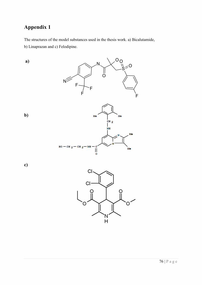
76 | P a g e
Appendix 1
The structures of the model substances used in the thesis work. a) Bicalutamide,
b) Linaprazan and c) Felodipine.
a)
b)
c)
FF
F
N
N
O
O
SO
O
F

77 | P a g e
Appendix 2
Nanocrystals of Bicalutamide
Preparations
Fill the water bath belonging to the S2 from Covaris with fresh MilliQ-water
Start the degas on the S2, at least 30 minutes prior to use
Prepare the stabilizer solution, 0.1(w/w) % AOT
Add 9 ml of MilliQ-water to a vial
Add one ml of 1(w/w) % AOT, wash the tip five times
Stir for 10 minutes
Filtrate the solution with a PTFE filter, 0.2m
Make the nanocrystals, 1mM Bicalutamide, 0.1(w/w) % AOT, 0.8(w/w) % DMSO
Add 1982L 0.1(w/w) % AOT solution to a Biotage microwave vial
Close the vial with parafilm
Put it in the S2
Prepare the addition of the stock solution, use a Hamilton syringe with a tall needle
Pull up the stock solution in the syringe, 16L 125mM Bicalutamide in DMSO
Draw some air into the needle
Dry the needle with Kleenex
Start the ”Ultrasonic” treatment
Rapidly add the stock solution
Put more parafilm on top of the vial
Put the lid on
When the run is finished measure the size

78 | P a g e
Appendix 3
Nanocrystals of Linaprazan
Preparations
Milling vessels, 1.2ml
Weigh in substance (~57mg)
o Add thawed vehicle, 1.33 (w/w) % PVP (K30), 0.067% (w/w) AOT to give 10
(w/w) % substance (~570mg)
o Add a magnet and let it stir over night
Weigh in 0.6-0.8mm zirconium beads (2*2.4g)
Milling
Add the “slurry” that has been stirred over night (or water) to the milling vessel (510mL)
Add the beads
Put the lid on
Put on parafilm to ensure tight closure of the vessles
Put the vessles in to the mill, Fritsch, Pulverisette, and attach them thoroughly
Start the Milling procedure
o 700rpm
o 4*30 minutes
o 15 minute brakes in-between
When finished, pull out the nanosuspension with a syringe and needle
Clean the beads with water; 3*1/2 volume (3*250L) to get as much compound as
possible
Use LC to determine the batch concentration
Measure the particle size

79 | P a g e
Appendix 4
Nanocrystals of Felodipine
Preparations
Fill the water bath belonging to the S2 from Covaris with fresh MilliQ-water
Start the degas on the S2, at least 30 minutes prior to use
Fill an ordinary ultrasound water bath with fresh MilliQ-water
Run for 5 minutes
Prepare the stabilizer solution, 0.1(w/w) % AOT
Add 9 ml of MilliQ-water to a vial
Add one ml of 1(w/w) % AOT, wash the tip five times
Mix it on a magnetic stirrer for 10 minutes
Filtrate the solution with a PTFE filter, 0.2m
Make the nanocrystals, 0.5mM Felodipine, 0.1(w/w) % AOT, 0.8(w/w) %DMSO
Add 1984L stabilizer solution to a Biotage microwave vial
Put the Biotage microwave vial in the ordinary ultrasonic bath, start it
Prepare the addition of the stock solution
Use a Hamilton syringe
Pull up the stock solution in the syringe, 16L 62.5mM Felodipine in DMSO
Draw some air into the needle
Dry the needle with Kleenex
Rapidly add the 16 L to the Biotage microwave vial
Put the lid on
Stop the ultrasound
Rapidly move it to the S2
Start the ”Ultrasonic” treatment
Put the lid on
When the run is finished measure the size
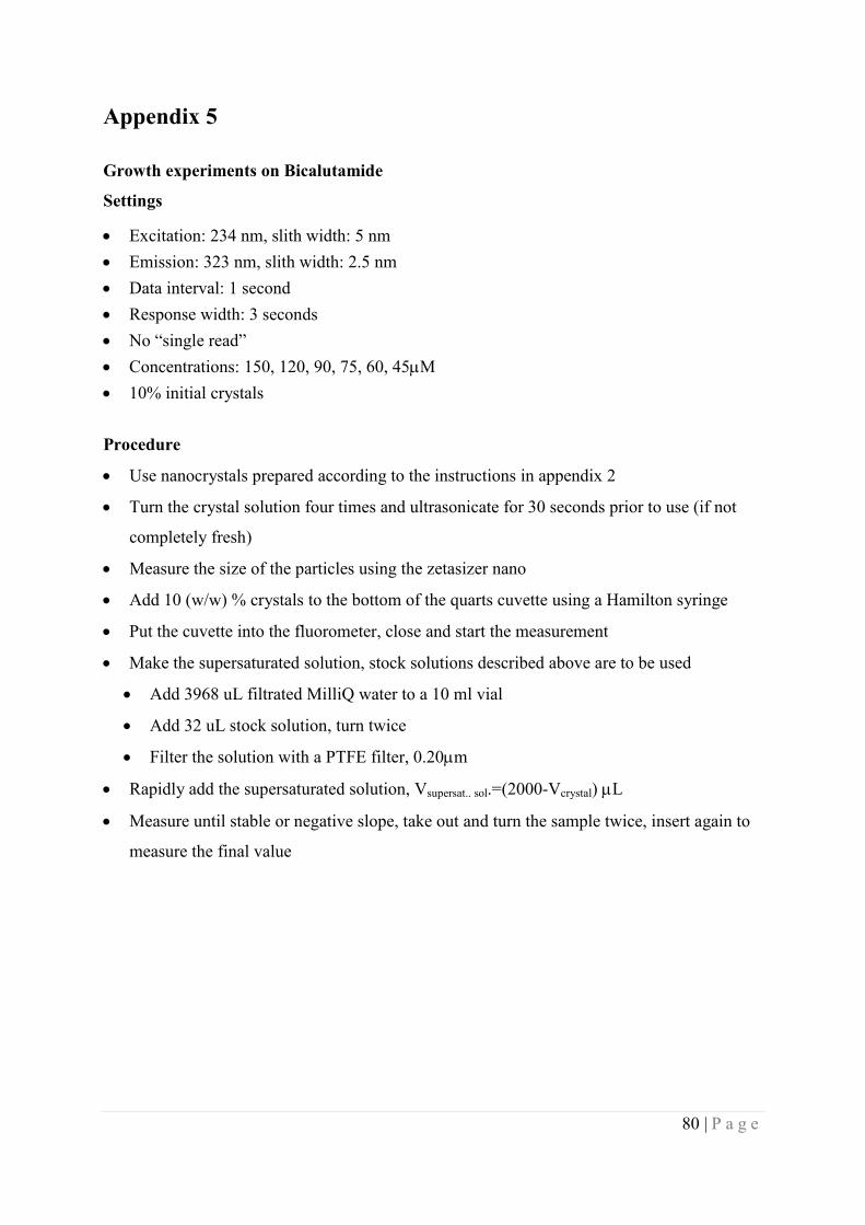
80 | P a g e
Appendix 5
Growth experiments on Bicalutamide
Settings
Excitation: 234 nm, slith width: 5 nm
Emission: 323 nm, slith width: 2.5 nm
Data interval: 1 second
Response width: 3 seconds
No “single read”
Concentrations: 150, 120, 90, 75, 60, 45M
10% initial crystals
Procedure
Use nanocrystals prepared according to the instructions in appendix 2
Turn the crystal solution four times and ultrasonicate for 30 seconds prior to use (if not
completely fresh)
Measure the size of the particles using the zetasizer nano
Add 10 (w/w) % crystals to the bottom of the quarts cuvette using a Hamilton syringe
Put the cuvette into the fluorometer, close and start the measurement
Make the supersaturated solution, stock solutions described above are to be used
Add 3968 uL filtrated MilliQ water to a 10 ml vial
Add 32 uL stock solution, turn twice
Filter the solution with a PTFE filter, 0.20m
Rapidly add the supersaturated solution, Vsupersat.. sol.=(2000-Vcrystal) L
Measure until stable or negative slope, take out and turn the sample twice, insert again to
measure the final value
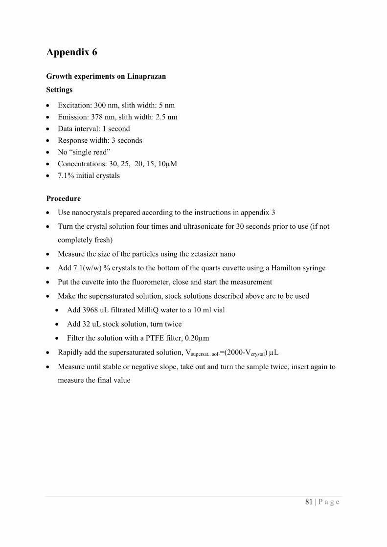
81 | P a g e
Appendix 6
Growth experiments on Linaprazan
Settings
Excitation: 300 nm, slith width: 5 nm
Emission: 378 nm, slith width: 2.5 nm
Data interval: 1 second
Response width: 3 seconds
No “single read”
Concentrations: 30, 25, 20, 15, 10M
7.1% initial crystals
Procedure
Use nanocrystals prepared according to the instructions in appendix 3
Turn the crystal solution four times and ultrasonicate for 30 seconds prior to use (if not
completely fresh)
Measure the size of the particles using the zetasizer nano
Add 7.1(w/w) % crystals to the bottom of the quarts cuvette using a Hamilton syringe
Put the cuvette into the fluorometer, close and start the measurement
Make the supersaturated solution, stock solutions described above are to be used
Add 3968 uL filtrated MilliQ water to a 10 ml vial
Add 32 uL stock solution, turn twice
Filter the solution with a PTFE filter, 0.20m
Rapidly add the supersaturated solution, Vsupersat.. sol.=(2000-Vcrystal) L
Measure until stable or negative slope, take out and turn the sample twice, insert again to
measure the final value
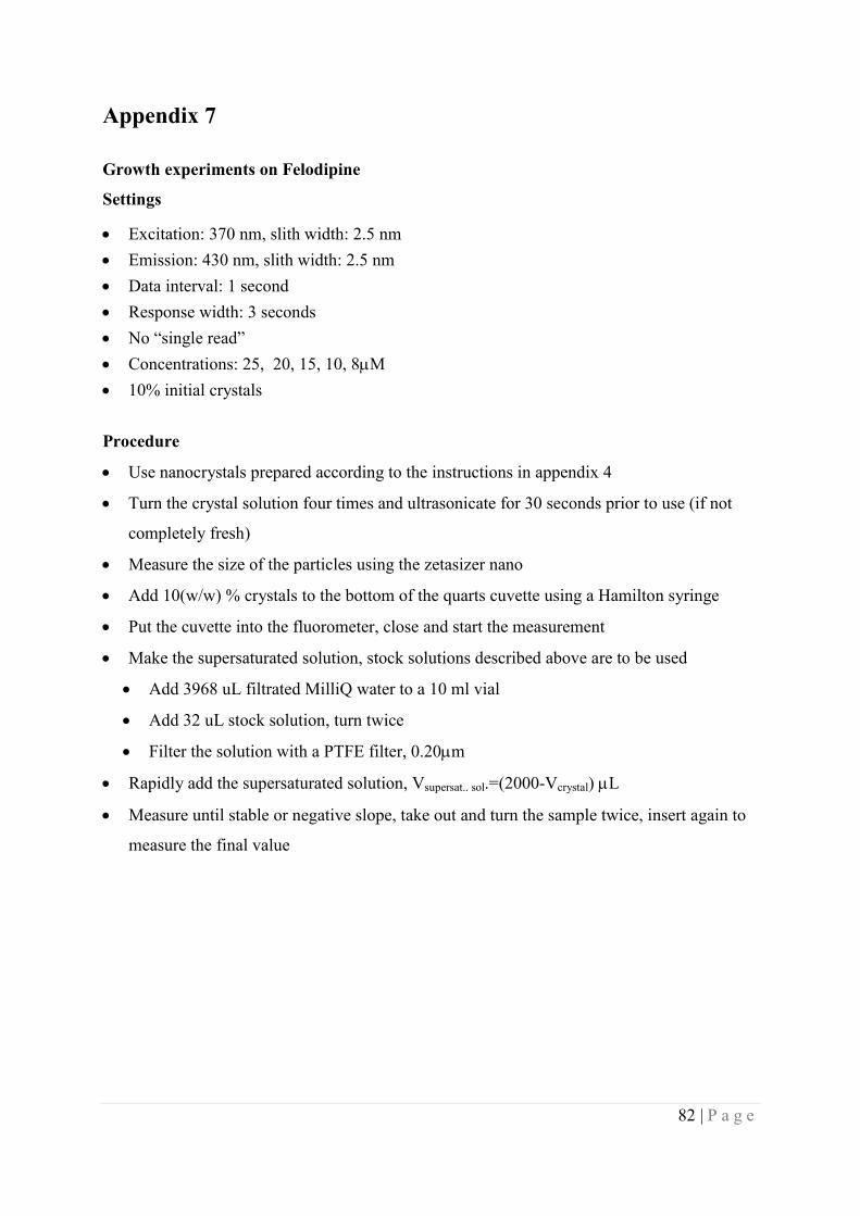
82 | P a g e
Appendix 7
Growth experiments on Felodipine
Settings
Excitation: 370 nm, slith width: 2.5 nm
Emission: 430 nm, slith width: 2.5 nm
Data interval: 1 second
Response width: 3 seconds
No “single read”
Concentrations: 25, 20, 15, 10, 8M
10% initial crystals
Procedure
Use nanocrystals prepared according to the instructions in appendix 4
Turn the crystal solution four times and ultrasonicate for 30 seconds prior to use (if not
completely fresh)
Measure the size of the particles using the zetasizer nano
Add 10(w/w) % crystals to the bottom of the quarts cuvette using a Hamilton syringe
Put the cuvette into the fluorometer, close and start the measurement
Make the supersaturated solution, stock solutions described above are to be used
Add 3968 uL filtrated MilliQ water to a 10 ml vial
Add 32 uL stock solution, turn twice
Filter the solution with a PTFE filter, 0.20m
Rapidly add the supersaturated solution, Vsupersat.. sol.=(2000-Vcrystal) L
Measure until stable or negative slope, take out and turn the sample twice, insert again to
measure the final value

83 | P a g e
Appendix 8
Dissolution experiments on Bicalutamide
Settings
Excitation: 234 nm, slith width: 5 nm
Emission: 323 nm, slith width: 5 nm
Data interval: 0.02 seconds
Response width: 0.06 seconds
No “single read”
Concentrations: 11.5, 8.5, 5.5, 2.5, 0M in the solution
1.5M initial crystals
Procedure
Use nanocrystals prepared according to the instructions in appendix 2
Turn the crystal solution four times and ultrasonicate for 30 seconds prior to use (if not
completely fresh)
Measure the size of the particles using the mastersizer
Add 1.5M crystals to the bottom of the quarts cuvette using a Hamilton syringe
Put the cuvette into the fluorometer, close and start the measurement
Make the undersaturated solution
Add 3968 uL filtrated MilliQ water to a 10 ml vial
Add 32 uL stock solution, turn twice
Filter the solution with a PTFE filter, 0.20m
Rapidly add the supersaturated solution to a total of 2ml
Measure until there is no slope

84 | P a g e
Appendix 9
Dissolution experiments on Linaprazan
Settings
Excitation: 300 nm, slith width: 5 nm
Emission: 378 nm, slith width: 5 nm
Data interval: 0.02 seconds
Response width: 0.06 seconds
No “single read”
Concentrations: 1.15, 0.85, 0.55, 0.35, 0.1, 0M in the solution
0.1M initial crystals
Procedure
Use nanocrystals prepared according to the instructions in appendix 3
Turn the crystal solution four times and ultrasonicate for 30 seconds prior to use (if not
completely fresh)
Measure the size of the particles using the mastersizer
Add 0.15M crystals to the bottom of the quarts cuvette using a Hamilton syringe
Put the cuvette into the fluorometer, close and start the measurement
Make the undersaturated solution
Add 3968 uL filtrated MilliQ water to a 10 ml vial
Add 32 uL stock solution, turn twice
Filter the solution with a PTFE filter, 0.20m
Rapidly add the supersaturated solution to a total of 2ml
Measure until there is no slope

85 | P a g e
Appendix 10
Dissolution experiments on Felodipine
Settings
Excitation: 370 nm, slith width: 5 nm
Emission: 430 nm, slith width: 5 nm
Data interval: 0.02 seconds
Response width: 0,06 seconds
No “single read”
Concentrations: 1.6, 1.2, 0.8, 0.4, 0.2, 0M in the solution
0.2M initial crystals
Procedure
Use nanocrystals prepared according to the instructions in appendix 4
Turn the crystal solution four times and ultrasonicate for 30 seconds prior to use (if not
completely fresh)
Measure the size of the particles using the mastersizer
Add 0.2M crystals to the bottom of the quarts cuvette using a Hamilton syringe
Put the cuvette into the fluorometer, close and start the measurement
Make the undersaturated solution
Add 3968 uL filtrated MilliQ water to a 10 ml vial
Add 32 uL stock solution, turn twice
Filter the solution with a PTFE filter, 0.20m
Rapidly add the supersaturated solution to a total of 2ml
Measure until there is no slope
86 | P a g e
Appendix 11
Crystal nucleation experiments on Bicalutamide – 440M /175M
Coat the plate
Prepare 1 (w/w) % (w/w) PVP solution (360 kDa), stir for a couple of hours
Filter with PTFE filter, 0,2m
Add 400µL to each well on the 96 microwell plate
Leave for two hours
Rinse ten times with tap-water
Rinse 5 times with MilliQ water
Put on a shaking table in a MilliQ water bath for a couple of hours
Rinse 5 times with MilliQ water
Dry the wells with nitrogen gas
Dry the plate in vacuum over night
Store upside down
Prepare the growth solution
Add 17.84 mL MilliQ water to a 20ml vial
Add 2000uL 0,21(w/w) % PVP (360 kDa), wash the tip five times
Carefully add 160 L 1.825mM Bicalutamide, turn twice
Filter with a PTFE filter, 0.2m
14.6M Bicalutamide, 0.021(w/w) % PVP 360kDa, 0.8(w/w) % DMSO
Nucleation experiment, nucleation at 440µM, growth at 175m, to be performed on
antivibration table
Check the plate, using the microscope
Add 193.1L of growth solution to each well by use of a manual pipette
Make supersaturated solutions, 440M
3968L filtered MilliQ water in a 10ml vial
Carefully add 32L, 55mM Bicalutamide, mix gently three times
Filter with a PTFE filter, 0.2m, in to a 4ml vial
tnuc

87 | P a g e
Transfer the solution to the plate
Calmly pull up the supersaturated solution, 116.9L, with a manual pipette
Put the solution down into a well, against the wall, calm and decisive. Pull up from the
bottom and down again against the wall
16 wells per nucleation time, 4 wells from each batch.
Growth time, 72 hours ( film+ cover + tinfoil)
6 series/ plate 0 min (reference), 15min, 30 min, 45 min, 60 min och 75 min.
Harvest the nucleation experiment
72 hours after the nucleation was terminated
Look at the wells by use of a light microscope, count the crystals and take photos of each
well
Evaluate using Sigma Plot and the Poisson distribution

88 | P a g e
Appendix 12
Crystal nucleation experiments on Linprazan – 30M /18M
Coat the plate
Prepare 1 (w/w) % HPMC solution (6 cPs), stir for a couple of hours
Filter with PTFE filter, 0,2m
Add 400µL to each well on the 96 microwell plate
Leave for two hours
Rinse ten times with tap-water
Rinse 5 times with MilliQ water
Put on a shaking table in a MilliQ water bath for a couple of hours
Rinse 5 times with MilliQ water
Dry the wells with nitrogen gas
Dry the plate in vacuum over night
Store upside down
Prepare the growth solution
Add 19.22 mL 1M NaOH to a 20ml vial
Add 500uL, 4(w/w) % HPMC (6 cPs), wash the tip five times
Carefully add 160 L 0.20mM Linprazan, turn twice
Filter with a PTFE filter, 0.2m
1.5M Linaprazan, 0.1(w/w) % HPMC (6cPs), 0.8(w/w) % DMSO, 1M NaOH
Nucleation experiment, nucleation at 30µM, growth at 18m, to be performed on
antivibration table
Check the plate, using the microscope
Add 130.5L of growth solution to each well by use of a manual pipette
Make supersaturated solutions, 30M
3968L filtered 1M NaOH in a 10ml vial
Carefully add 32L, 4mM Linaprazan, mix gently three times
Filter with a PTFE filter, 0.2m, in to a 4ml vial
tnuc

89 | P a g e
Transfer the solution to the plate
Calmly pull up the supersaturated solution, 179.5L, with a manual pipette
Put the solution down into a well, against the wall, calm and decisive. Pull up from the
bottom and down again against the wall
16 wells per nucleation time, 4 wells from each batch.
Growth time, 72 hours ( film+ cover + tinfoil)
6 series/ plate 0 min (reference), 1, 2, 4, 6 and 8 hours.
Harvest the nucleation experiment
72 hours after the nucleation was terminated
Look at the wells by use of a light microscope, count the crystals and take photos of each
well
Evaluate using Sigma Plot and the Poisson distribution

90 | P a g e
Appendix 13
Result from the mastersizer measurement on Bicalutamide nanoparticles- after editing.
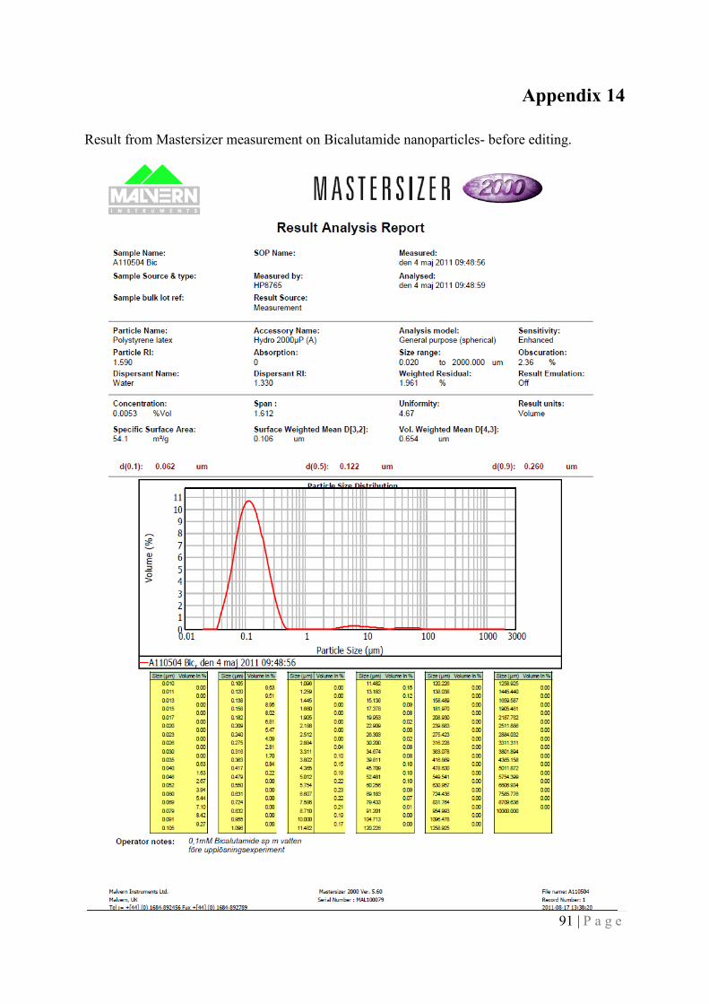
91 | P a g e
Appendix 14
Result from Mastersizer measurement on Bicalutamide nanoparticles- before editing.

92 | P a g e
Appendix 15
Result from the mastersizer measurement on Linaprazan nanoparticles- after editing.

93 | P a g e
Appendix 16
Result from the mastersizer measurement on Linaprazan nanoparticles- before editing.

94 | P a g e
Appendix 17
Result from the mastersizer measurement on Felodipine nanoparticles- after editing.

95 | P a g e
Appendix 18
Result from the mastersizer measurement on Felodipine nanoparticles- before editing.
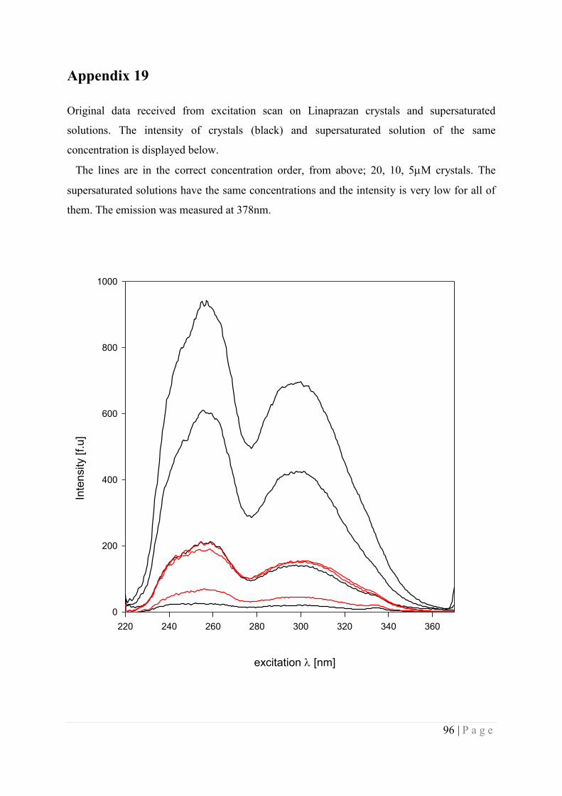
96 | P a g e
Appendix 19
Original data received from excitation scan on Linaprazan crystals and supersaturated
solutions. The intensity of crystals (black) and supersaturated solution of the same
concentration is displayed below.
The lines are in the correct concentration order, from above; 20, 10, 5M crystals. The
supersaturated solutions have the same concentrations and the intensity is very low for all of
them. The emission was measured at 378nm.
220 240 260 280 300 320 340 360
0
200
400
600
800
1000
excitation [nm]
Inte
nsity [
f.u
]

97 | P a g e
Appendix 20
Results from the comparison between the crystal dissolution experiments on Bicalutamide
and classic nucleation theory. The mean value is displayed along with the standard error of
the mean. The solid lines are the simulated curves. Note the difference in scale of the y-axis.
a) b)
c) d)
Time [seconds]
0 10 20 30 40 50 60
Fra
ction c
rysta
lline m
ate
rial
0.00
0.02
0.04
0.06
0.08
0.10
0.12
0 10 20 30 40 50 60
0.00
0.02
0.04
0.06
0.08
0.10
0.12
0.14
Time [seconds]
Fra
ction c
rysta
lline m
ate
rial
0 10 20 30 40 50 60
0.00
0.05
0.10
0.15
0.20
Time [seconds]
Fra
ctio
n c
rysta
llin
e m
ate
ria
l
0 10 20 30 40 50 60
0.0
0.1
0.2
0.3
0.4
Time [seconds]
Fra
ctio
n c
rysta
llin
e m
ate
ria
l

98 | P a g e
e)
a) 11.5M Bicalutamide in the solution and 1.5M initial crystals,=0m
b) 8.5M Bicalutamide in the solution and 1.5M initial crystals,=0m
c) 5.5M Bicalutamide in the solution and 1.5M initial crystals,=0m
d) 2.5M Bicalutamide in the solution and 1.5M initial crystals,=0m
e) 0M Bicalutamide in the solution and 1.5M initial crystals,=0m
Time [seconds]
0 10 20 30 40 50 60
Fra
ction c
rysta
lline m
ate
rial
0.0
0.2
0.4
0.6
0.8
1.0
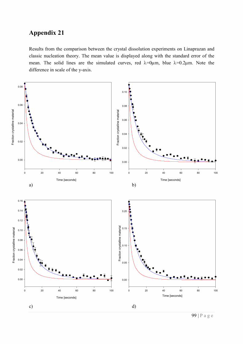
99 | P a g e
Appendix 21
Results from the comparison between the crystal dissolution experiments on Linaprazan and
classic nucleation theory. The mean value is displayed along with the standard error of the
mean. The solid lines are the simulated curves, red =0m, blue =0.2m. Note the
difference in scale of the y-axis.
a) b)
c) d)
0 20 40 60 80 100
0.00
0.02
0.04
0.06
0.08
Time [seconds]
Fra
ction c
rysta
lline m
ate
rial
0 20 40 60 80 100
0.00
0.02
0.04
0.06
0.08
0.10
Time [seconds]
Fra
ction
cry
sta
lline
mate
rial
0 20 40 60 80 100
0.00
0.02
0.04
0.06
0.08
0.10
0.12
0.14
0.16
Time [seconds]
Fra
ction
cry
sta
lline
mate
rial
0 20 40 60 80 100
0.00
0.05
0.10
0.15
0.20
Time [seconds]
Fra
ction c
rysta
lline m
ate
rial
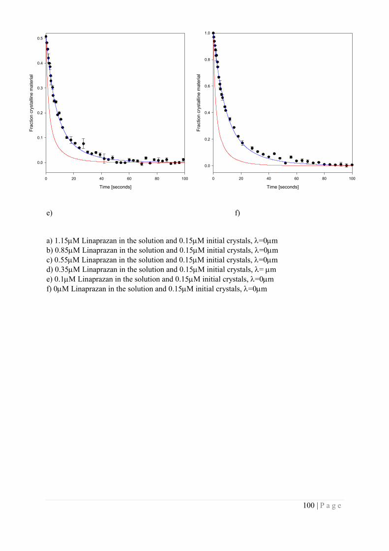
100 | P a g e
e) f)
a) 1.15M Linaprazan in the solution and 0.15M initial crystals,=0m
b) 0.85M Linaprazan in the solution and 0.15M initial crystals,=0m
c) 0.55M Linaprazan in the solution and 0.15M initial crystals,=0m
d) 0.35M Linaprazan in the solution and 0.15M initial crystals,=m
e) 0.1M Linaprazan in the solution and 0.15M initial crystals,=0m
f) 0M Linaprazan in the solution and 0.15M initial crystals,=0m
0 20 40 60 80 100
0.0
0.1
0.2
0.3
0.4
0.5
Time [seconds]
Fra
ction
cry
sta
lline
mate
rial
Time [seconds]
0 20 40 60 80 100
Fra
ctio
n c
rysta
llin
e m
ate
ria
l
0.0
0.2
0.4
0.6
0.8
1.0

101 | P a g e
0 20 40 60 80 100 120
0.00
0.05
0.10
0.15
0.20
0.25
Time [seconds]
Fra
ctio
n c
rysta
llin
e m
ate
ria
l
0 20 40 60 80 100 120
0.0
0.1
0.2
0.3
Time [seconds]
Fra
ction c
rysta
lline m
ate
rial
Appendix 22
Results from the comparison between the crystal dissolution experiments on Linaprazan and
classic nucleation theory. The mean value is displayed along with the standard error of the
mean. The solid lines are the simulated curves. Note the difference in scale of the x and y-axis.
a) b)
b) d)
0 20 40 60 80 100 120 140 160
0.00
0.02
0.04
0.06
0.08
0.10
0.12
0.14
0.16
Time [seconds]
Fra
ctio
n c
rysta
llin
e m
ate
ria
l
0 20 40 60 80 100 120 140 160
0.00
0.02
0.04
0.06
0.08
0.10
0.12
Time [seconds]
Fra
ctio
n c
rysta
lline
mate
rial
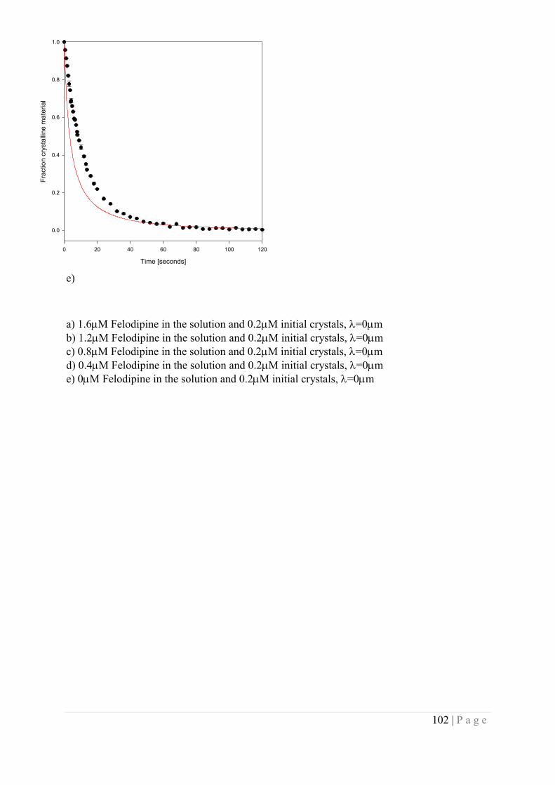
102 | P a g e
e)
a) 1.6M Felodipine in the solution and 0.2M initial crystals,=0m
b) 1.2M Felodipine in the solution and 0.2M initial crystals,=0m
c) 0.8M Felodipine in the solution and 0.2M initial crystals,=0m
d) 0.4M Felodipine in the solution and 0.2M initial crystals,=0m
e) 0M Felodipine in the solution and 0.2M initial crystals,=0m
Time [seconds]
0 20 40 60 80 100 120
Fra
ctio
n c
rysta
llin
e m
ate
ria
l
0.0
0.2
0.4
0.6
0.8
1.0
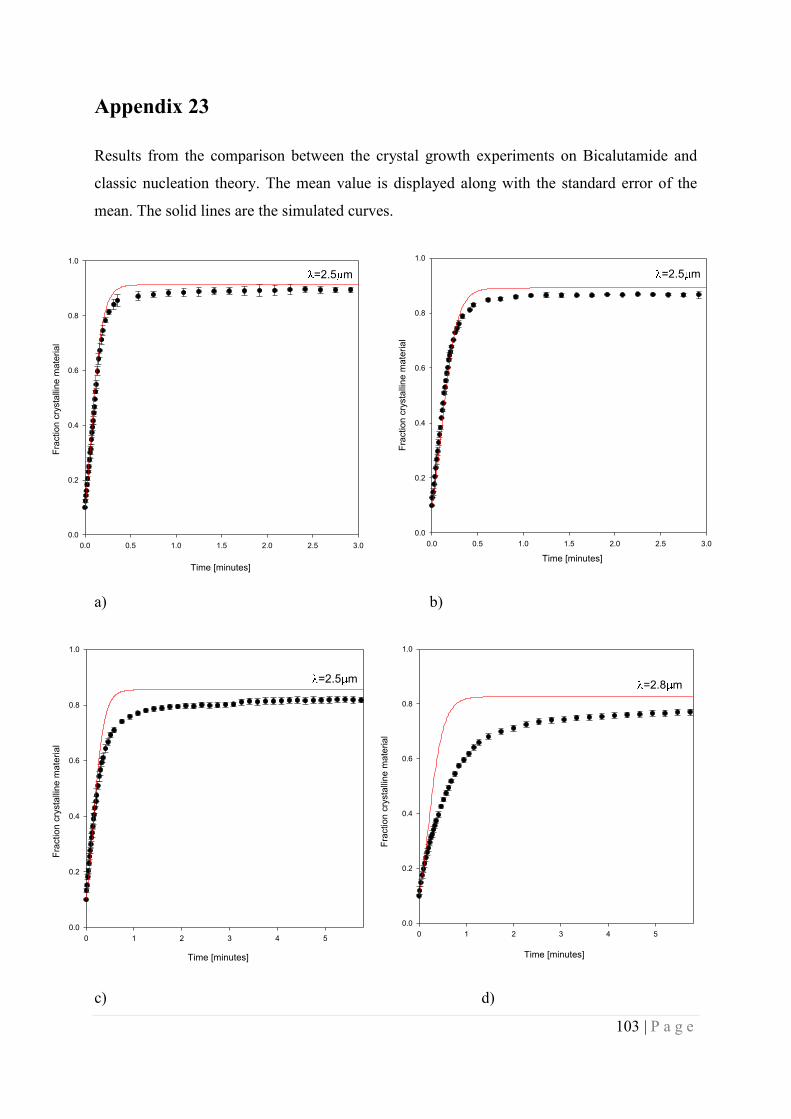
103 | P a g e
Appendix 23
Results from the comparison between the crystal growth experiments on Bicalutamide and
classic nucleation theory. The mean value is displayed along with the standard error of the
mean. The solid lines are the simulated curves.
a) b)
c) d)
Time [minutes]
0.0 0.5 1.0 1.5 2.0 2.5 3.0
Fra
ction c
rysta
lline m
ate
rial
0.0
0.2
0.4
0.6
0.8
1.0
=2.5 m
0.0 0.5 1.0 1.5 2.0 2.5 3.0
0.0
0.2
0.4
0.6
0.8
1.0
Time [minutes]
Fra
ctio
n c
rysta
llin
e m
ate
ria
l
=2.5 m
0 1 2 3 4 5
0.0
0.2
0.4
0.6
0.8
1.0
Time [minutes]
Fra
ctio
n c
rysta
llin
e m
ate
ria
l
=2.5 m
0 1 2 3 4 5
0.0
0.2
0.4
0.6
0.8
1.0
Time [minutes]
Fra
ctio
n c
rysta
llin
e m
ate
ria
l
=2.8 m

104 | P a g e
e) f)
a) 150M supersaturated solution with 10% initial crystalline material, =2.5m
b) 120M supersaturated solution with 10% initial crystalline material, =2.5m
c) 90 M supersaturated solution with 10% initial crystalline material, =2.5m
d) 75M supersaturated solution with 10% initial crystalline material, =2.5m
e) 60M supersaturated solution with 10% initial crystalline material, =6m
f) 45M supersaturated solution with 10% initial crystalline material, =30m.
0 20 40 60 80
0.0
0.2
0.4
0.6
0.8
1.0
Time [minutes]
Fra
ctio
n c
rysta
llin
e m
ate
ria
l
=6.0 m
0 20 40 60 80
0.0
0.2
0.4
0.6
0.8
1.0
Time [minutes]
Fra
ctio
n c
rysta
llin
e m
ate
ria
l
=30 m
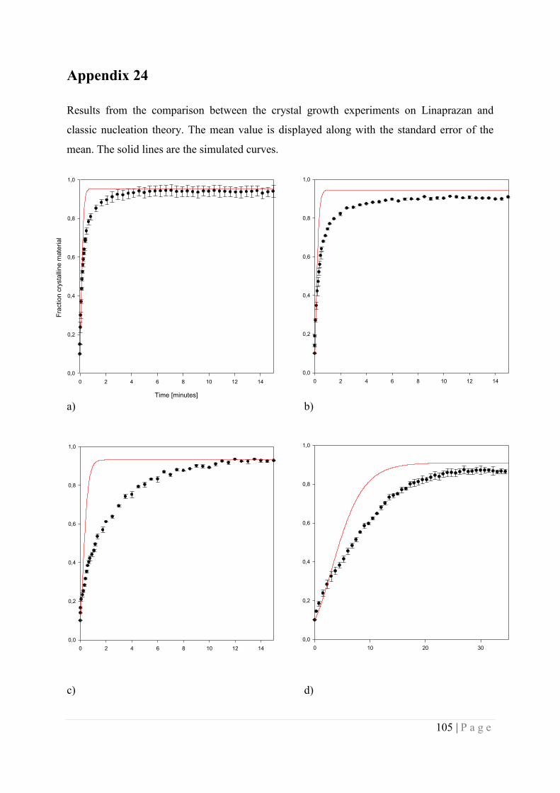
105 | P a g e
Appendix 24
Results from the comparison between the crystal growth experiments on Linaprazan and
classic nucleation theory. The mean value is displayed along with the standard error of the
mean. The solid lines are the simulated curves.
a) b)
c) d)
Time [minutes]
0 2 4 6 8 10 12 14
Fra
ction c
rysta
lline m
ate
rial
0,0
0,2
0,4
0,6
0,8
1,0
0 2 4 6 8 10 12 14
0,0
0,2
0,4
0,6
0,8
1,0
0 2 4 6 8 10 12 14
0,0
0,2
0,4
0,6
0,8
1,0
0 10 20 30
0,0
0,2
0,4
0,6
0,8
1,0
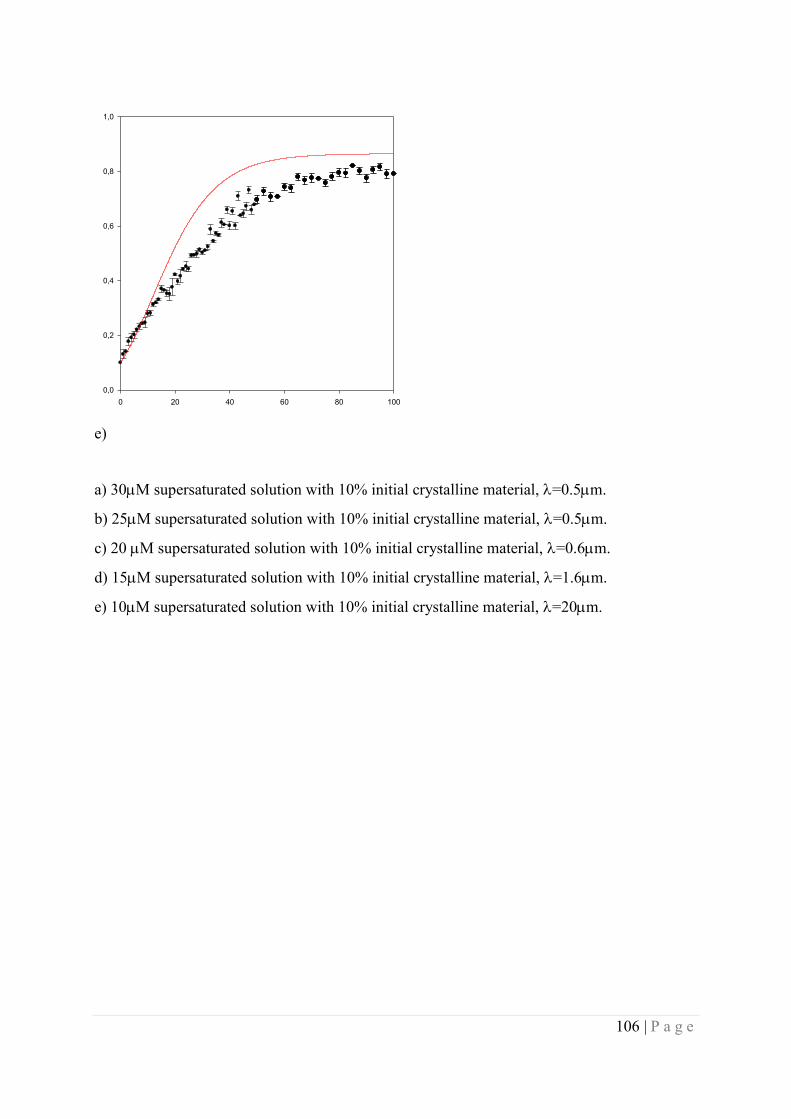
106 | P a g e
e)
a) 30M supersaturated solution with 10% initial crystalline material, =0.5m.
b) 25M supersaturated solution with 10% initial crystalline material, =0.5m.
c) 20 M supersaturated solution with 10% initial crystalline material,=0.6m.
d) 15M supersaturated solution with 10% initial crystalline material,=1.6m.
e) 10M supersaturated solution with 10% initial crystalline material,=20m.
0 20 40 60 80 100
0,0
0,2
0,4
0,6
0,8
1,0

107 | P a g e
Appendix 25
Results from the comparison between the crystal growth experiments on Felodipine and
classic nucleation theory. The mean value is displayed along with the standard error of the
mean. The solid lines are the simulated curves.
a) b)
c) d)
0 10 20 30
0,0
0,2
0,4
0,6
0,8
1,0
0 10 20 30
0,0
0,2
0,4
0,6
0,8
1,0
0 10 20 30 40
0,0
0,2
0,4
0,6
0,8
1,0
0 20 40 60 80 100 120 140
0,0
0,2
0,4
0,6
0,8
1,0
108 | P a g e
a) 25M supersaturated solution with 10% initial crystalline material, =3.5m.
b) 20M supersaturated solution with 10% initial crystalline material, =2.8m.
c) 15 M supersaturated solution with 10% initial crystalline material, =3.0m.
d) 10M supersaturated solution with 10% initial crystalline material, =7m.
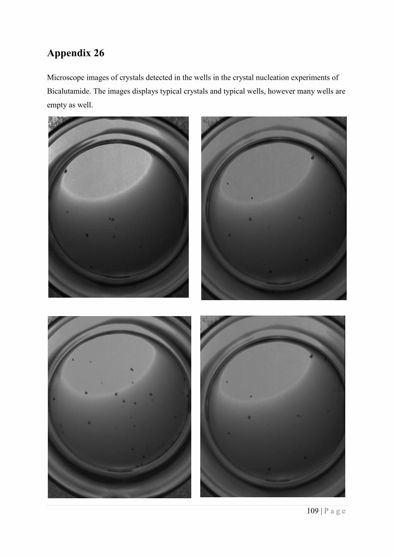
109 | P a g e
Appendix 26
Microscope images of crystals detected in the wells in the crystal nucleation experiments of
Bicalutamide. The images displays typical crystals and typical wells, however many wells are
empty as well.

110 | P a g e
Appendix 27
Microscope images of crystals detected in the wells in the crystal nucleation experiments of
Linaprazan. The images displays typical crystals and typical wells, however many wells are
empty as well.

111 | P a g e

![REVIEW ON SOLUBILITY ENHANCEMENT TECHNIQUES...absorption of poorly water-soluble drugs. [8,9] In solid dispersion a poorly soluble drug is dispersed in a highly soluble solid hydrophilic](https://static.fdocuments.net/doc/165x107/5fab6e219a0b2d27a86e8e9a/review-on-solubility-enhancement-techniques-absorption-of-poorly-water-soluble.jpg)