Cryptocurrencies, gold, and WTI crude oil market ...

Cryptocurrencies, gold, and WTI crude oil market efficiency: a dynamic analysis based on the adaptive market hypothesisMajid Mirzaee Ghazani* and Mohammad Ali Jafari

IntroductionThe substantial growth of cryptocurrencies has attracted considerable attention from investors and policymakers in recent years. As of June 5, 2019, this growth topped 2216 cryptocurrencies in market capitalization and volume of trade, and the top three coins, Bitcoin, Ethereum, and Ripple, together accounted for more than 70 percent of the mar-ket share (Cryptocurrency Market Capitalizations 2019).

One of the critical issues yet to be analyzed is whether the dynamic behavior of crypto-currencies is predictable, which would be inconsistent with the efficient market hypoth-esis (EMH), according to which prices should follow a random walk (see Fama 1970). Long-memory techniques can be applied for this purpose. In the meantime, numerous studies have provided evidence of the persistent behavior of asset prices (see Caporale et al. 2016)1 and have also found that this behavior varies over time, but few studies have focused on the cryptocurrency market. One of the few exceptions is the work of Bouri et al. (2016), who discovered long memory properties in the volatility of Bitcoin.

Abstract

This study examined the evolving oil market efficiency by applying daily historical data to the three benchmark cryptocurrencies (Bitcoin, Ethereum, and Ripple), gold, and West Texas Intermediate (WTI) crude oil. The data coverage of daily returns was from August 2015 to April 2019. We applied two alternative tests to examine linear and nonlinear dependency, i.e., automatic portmanteau and generalized spectral tests. The analysis of observed results validated the adaptive market hypothesis (AMH) in all markets, but the degree of adaptability between the data was different. In this study, we also analyzed the existence of evolutionary behavior in the market. To achieve this goal, we checked the results by applying the rolling-window method with three differ-ent window lengths (50, 100, and 150 days) on the test statistics, which was consistent with the findings of AMH.

Keywords: Adaptive market hypothesis, Market efficiency, Cryptocurrency, Evolutionary, Rolling windows

Open Access

© The Author(s), 2021. Open Access This article is licensed under a Creative Commons Attribution 4.0 International License, which permits use, sharing, adaptation, distribution and reproduction in any medium or format, as long as you give appropriate credit to the original author(s) and the source, provide a link to the Creative Commons licence, and indicate if changes were made. The images or other third party material in this article are included in the article’s Creative Commons licence, unless indicated otherwise in a credit line to the mate-rial. If material is not included in the article’s Creative Commons licence and your intended use is not permitted by statutory regulation or exceeds the permitted use, you will need to obtain permission directly from the copyright holder. To view a copy of this licence, visit http:// creat iveco mmons. org/ licen ses/ by/4. 0/.

RESEARCH

Ghazani and Jafari Financ Innov (2021) 7:29 https://doi.org/10.1186/s40854-021-00246-0 Financial Innovation

*Correspondence: [email protected] Department of Industrial Engineering, K. N. Toosi University of Technology, Tehran, Iran

1 In this regard, we refer to some studies that have analyzed the financial markets through different aspects and meth-ods (e.g., Kou et al. 2014, 2019; Chao et al. 2019).

http://orcid.org/0000-0002-7606-9464

http://creativecommons.org/licenses/by/4.0/

http://creativecommons.org/licenses/by/4.0/

http://crossmark.crossref.org/dialog/?doi=10.1186/s40854-021-00246-0&domain=pdf

of 26Ghazani and Jafari Financ Innov (2021) 7:29

Most of the existing studies concerning market efficiency in financial assets have accepted weak-form efficiencies (see Fama 1970). The notion of efficient financial mar-kets is a well-established topic in finance and economics. The concept of market effi-ciency was discussed over the past five decades since Fama (1970) first introduced the renowned EMH concept. In earlier years of analyzing the market efficiency; it focused on stochastic processes of asset price fluctuations. The reasoning behind market effi-ciency was that asset prices in an efficient market should follow a random-walk pro-cess because all available information about the prices was already mirrored in the asset price. Therefore, asset prices could not be forecasted based on a recent series of data. Thus, gathering information in an efficient market would not be effective because new information would immediately change its price. Grossman and Stiglitz (1980) argued that a perfect market is unfeasible because if prices expressed all available information, traders would have no incentive to obtain costly information. In other words, if a market shows weak-form efficiency, then returns are not forecastable and must be independent of each other (Fama 1970). In contrast, if prices are forecastable and dependent, traders can utilize them to obtain abnormal profits.

Several papers have shown that asset prices do not accompany random walks and that price fluctuations are forecastable (Fama and French 1988). Diverse trading strategies can be utilized based on these forecasted variances in returns (Jegadeesh and Titman 1993). This finding has caused a burgeoning of literature to scrutinize the viability of the EMH notion in different countries (see Opong et al. 1999; Borges 2010). These studies have applied statistical tests to assess whether a market is efficient over some predeter-mined periods with the result that market efficiency can be used under all-or-nothing circumstances. A dispute exists between recent literature and EMH because studies have found that market oddities do exist as returns have a dependent feature (see Shahid and Mehmood 2015). These studies have demonstrated that the stock exchanges have some abnormal profits. A theoretical approach has confirmed this dispute, as Grossman and Stiglitz (1980) debated that it is impracticable for a capital market to be perfectly effi-cient because investors would have no advantage to obtain costly information if markets were efficient and profit-making opportunities were not available. Regarding the aspect of the impossibility of a perfectly efficient market, Campbell et al. (1997) suggested rela-tive efficiency rather than perfect efficiency, which causes an oscillation from testing the market’s efficiency from an all-or-nothing condition to evaluate it over the period.

Moreover, these findings and recently developed empirical literature have indicated that market efficiency changes over time (see Lim and Brooks 2011). These studies have challenged the viability of the EMH and suggest that it does not regularly hold.

This continued debate about the EMH has been furthered by reasoning from behavio-ral finance specialists about the central assumption of the EMH (the rationality perspec-tive of investors).

Furthermore, Lo (2004) expanded on behavioral biases based on Simon’s (1955) concept of bounded rationality. Bearing in mind the sociological attitude of the EMH argument, an alternative approach may be required rather than the standard deductive method of neoclassical economics, which is bounded by rationality. A new approach was suggested by Farmer and Lo (1999), and Farmer (2002) applied evolutionary concepts to financial markets. Lo (2005) disputed that moving to a state of equilibrium was neither


likely to happen nor assured at any point in the future periods. Undoubtedly, it is errone-ous to assume that the market has to adjust its position toward a stable equilibrium state or a perfect efficiency. Alternatively, the new paradigm (suggested in follows), offers more sophisticated market dynamics, such as cycles, crashes, trends, bubbles, and other developments in the financial market, resulting in market inefficiency (Lo 2005).

On this subject, Lo (2004) proposed the concept of the adaptive market hypothesis (AMH) to assert that market efficiency and inefficiencies coexist in a reasonably consist-ent manner. Moreover, the AMH permits market efficiency to oscillate over time and does not suggest an all-or-nothing arrangement.

The AMH borrows from the notion of evolution in biology and bounded rational-ity (Simon 2000) and debates that, by rational entities, the processes of competition, learning, and natural selection push prices to approach their efficient values. As market participants adjust to an evolving environment, they count on heuristics to build their investment choices.

The AMH offers an essential theoretical foundation to bring together behavioral models with EMH to explain the anomalies. Note that numerous examples indicate the breaches of rationality that conflict with market efficiency (e.g., overconfidence, loss aversion, mental accounting, overreaction, and other behavioral biases). As long as there may be arbitrage opportunities in the market, these anomalies would disappear as they are detected and used by the market participants, and new opportunities may arise. These conducts are consistent with an evolutionary model of individuals adapting to a changing environment through simple heuristics. In addition, the occurrences that alter financial market situations (e.g., crashes, bubbles) influence participants’ psycho-logical process in the market through which they absorb the new information into prices (Charles et al. 2012).

Considering these arguments, in this study, we assessed the market efficiency’s evo-lutionary behavior in regard to selected cryptocurrencies, gold, and West Texas Inter-mediate (WTI) oil prices in the AMH framework. We selected gold and WTI crude oil along with cryptocurrencies for the following reasons: In the finance literature, differ-ent roles have been expressed for gold, including a surrogate currency, a hedging tool against inflation, and a safe-haven asset, as well as its use in achieving greater risk diver-sification in investors’ portfolios. These factors have received increased attention from policymakers, portfolio investors, and risk managers. Another asset that investors are usually interested in is crude oil, which is an essential commodity that also has been commonly used to hedge against economic risks. The rise of commodity financializa-tion since 2005 (Lei et al. 2019; Chen et al. 2018; Tang and Xiong 2012) and the impact of oil price changes on the real economy and financial markets have been investigated extensively in the literature (Hamilton 1996; Jones and Kaul 1996; Kilian and Park 2009). In addition, WTI crude oil is a benchmark in this area and is also a critical component in most energy and commodity indices in financial markets.

Literature reviewA critical implication of the AMH is that individual preferences adjust over time, and accordingly, the risk premia are likewise time-varying. This phenomenon brings in a testable hypothesis that the autocorrelation in return series has a time-varying structure


and is conditioned to the financial market’s circumstance (Kim et al. 2011; Baur et al. 2012). Identical results for the AMH are expressed in the framework of other asset mar-kets, such as energy derivatives (Hall et al. 2017), foreign exchange (Charles et al. 2012), and real estate investment trust (REIT; Zhou and Lee 2013).

Noda (2016) analyzed the AMH in Japanese stock markets (TOPIX and TSE2) and measured the degree of market efficiency by applying a time-varying model. The obtained results showed that (1) the degree of market efficiency changed over time in the two markets, (2) the level of market efficiency of the TSE2 was lower than that of the TOPIX in most periods, and (3) the evolving behavior was recognizable in the market efficiency of the TOPIX index, but that of the TSE2 was not. Finally, the findings backed the AMH for the more qualified stock market (TOPIX) in Japan.

Numapau Gyamfi (2018) analyzed the return predictability of two stock indices (the GSEFSII and the GSEALSH) on the Ghana stock market. This study analyzed results from a return series in 2011–2015 by applying the generalized spectral (GS) test, the wild-bootstrapped automatic variance ratio test, and the automatic portmanteau (AP) Box–Pierce test. The obtained results showed that the GSEALSH index was more fore-seeable than the GSEFSII index in all of the tests. Moreover, the author concluded that his findings were consistent with the AMH.

Some of the recent research has focused on analyzing the market efficiency of cryp-tocurrencies, and benchmark financial assets and interconnections have been stated. Urquhart (2016) studied the Bitcoin market from its beginnings in 2010 to mid-2016 and suggested that the market was inefficient, but it moved closer toward efficiency in time. Nadarajah and Chu (2017) disputed these results and concluded that the market was, in fact, efficient. Bariviera (2017) applied the detrended fluctuation analysis (DFA) method to check dependence properties of the Bitcoin price and found a trend toward efficiency and that the volatility of Bitcoin had long-term memory throughout the sample period.

Wei (2018) evaluated the connection between liquidity and market efficiency in 456 different cryptocurrencies. His work showed that Bitcoin returns showed signs of effi-ciency, but several cryptocurrencies still displayed inefficiency in their prices. Moreover, the results of this study indicated that liquidity played a vital role in the market efficiency and return predictability of new cryptocurrencies.

Caporale et al. (2018) examined the market efficiency in the cryptocurrency market by checking data persistence. They applied the four leading cryptocurrencies (Bitcoin, Lite-coin, Ripple, and Dash) over the sample period, i.e., 2013–2017. Their findings suggested that this market showed persistence and that its degree fluctuated over time. Therefore, based on the predictability of data, they inferred that the market was inefficient, and traders could attain abnormal profits in this situation.

Khuntia and Pattanayak (2018) evaluated the AMH and return predictability in the Bitcoin market. They applied two different methods to capture time-varying linear and nonlinear dependence in Bitcoin returns. Their finding was that the market efficiency changed with time and confirmed the AMH in the Bitcoin market.

Kristoufek (2018) examined the efficiency of two Bitcoin markets and their evolving behavior over time. They applied the efficiency index of Kristoufek and Vosvrda (2013), which involved numerous types of (in)efficiency measures. Their study’s notable finding was that there was strong evidence of both Bitcoin markets remaining mostly inefficient


between 2010 and 2017 with the exceptions of several periods (after the observation of a bubble-like price increase).

Zhang et al. (2018) verified the issue of informational efficiency in the cryptocurrency market by evaluating nine forms of cryptocurrencies (i.e., Bitcoin, Ripple, Ethereum, NEM, Stellar, Litecoin, Dash, Monero, and Verge) according to efficiency tests. The empirical results in their study exhibited inefficiency in all of these cryptocurrencies markets.

Corbet et al. (2018) examined the interactions between three well-known cryptocur-rencies and various other financial assets. They found evidence of the relative isolation of these assets from the financial and economic assets. In addition, their results showed that cryptocurrencies may offer diversification benefits for investors with short invest-ment horizons and that time variation in the linkages reflect external economic and financial shocks.

Gajardo et al. (2018) applied multifractal adjusted detrended cross-correlation analy-sis (MF-ADCCA) to investigate the presence and asymmetry of the cross-correlations among the major currencies and Bitcoin, the Dow Jones Industrial Average (DJIA), the price of gold, and the crude oil market. They observed that multifractality existed in every cross-correlation studied and that there was an asymmetry in the cross-correla-tion exponents in the data. Bitcoin showed more significant multifractal spectra than the other currencies on its cross-correlation with the WTI, gold, and the DJIA. The authors concluded that Bitcoin had a different relationship with stock market indices and com-modities, which should be considered when investing.

Ghazani and Ebrahimi (2019) investigated the existence of the AMH by utilizing daily returns from 2003 to 2018 for three crude oils: Brent, WTI, and Organization of the Petroleum Exporting Countries (OPEC) basket. The findings indicated that the WTI and the Brent oil markets had the topmost efficiency levels. OPEC basket behavior demon-strated that by moving toward longer window lengths, the extent of compliance with AMH decreased.

Jin et al. (2019) argued that in a system containing three commonly used hedging assets (i.e., Bitcoin, gold, and crude oil), they would be able to recognize which one was more informative in clarifying price oscillations. Three different methods, multifractal detrended cross-correlation analysis (MF-DCCA), information share (IS) analysis, and multivariate GARCH (MVGARCH), were utilized to reach this goal. The results illus-trated that (1) the MF-DCCA suggested that multifractality existed in the cross-correla-tions among the three hedging assets, and Bitcoin was more prone to price fluctuations than gold and crude oil markets. (2) The dynamic correlations between gold and crude oil markets were almost positive, whereas those between Bitcoin and gold and between Bitcoin and oil markets were nearly negative.

Kang et al. (2019) utilized wavelet coherence and dynamic conditional correlations (DCCs) to analyze the hedging and diversification properties of Bitcoin prices in regard to gold futures. They examined whether the bubble patterns in gold futures prices could be utilized to hedge against the same behavior in the Bitcoin market in the short-term, and vice versa. They also examined whether each could be employed to manage and hedge the overall market and the sector downside risk of the other asset or commodity. The wavelet coherence results indicated a relatively high degree of comovement across


the 8- to 16-week frequency band between Bitcoin and gold futures prices for the 2012–2015 time period.

Noda (2020) investigated whether the market efficiency of selected cryptocurren-cies (Bitcoin and Ethereum) changed over time based on the AMH. He measured the extent of market efficiency by applying a time-varying model that did not have any type of dependency upon sample size, unlike prior studies that utilized common approaches. The empirical findings indicated that (1) the extent of market efficiency fluctuated with time in the markets, (2) the level of Bitcoin’s market efficiency was higher than that of Ethereum over most of the periods, and (3) a market with high market liquidity was evolving. Generally, the findings supported the AMH for the most well-established cryp-tocurrency market.

Tran and Leirvik (2020) applied a method to quantify the level of market efficiency, the so-called adjusted market inefficiency magnitude (AMIM; see Tran and Leirvik 2019). They showed that the level of market efficiency in the five largest cryptocurrencies was highly time-varying. Their study noted two reasons for this phenomenon. First, by applying a longer sample than previous studies and, second, by implementing a robust measure of efficiency, they were able to determine directly whether the efficiency was significant. They concluded that Litecoin was the most efficient cryptocurrency, and Ripple was the least efficient one.

Tripathi et al. (2020) investigated the AMH for 21 major global market indices for 1998–2018. They employed quantile-regression methodology to scrutinize the market efficiency of 16 financial markets. The findings showed that the returns in higher quan-tiles were negatively autocorrelated, and those in lower quantiles were positively auto-correlated. In general, market efficiency seemed to be time-varying and conditioned to the state of the market. Moreover, the analysis suggested significant evidence supporting the AMH for a considerable number of financial markets.

Varghese and Madhavan (2020) investigated the long memory dynamics in crude oil markets from an AMH perspective. In doing so, they selected the three benchmark crude oils, namely, WTI, Brent, and Dubai crude prices, for a rolling Hurst exponent analysis. Their findings showed the WTI market to be the most efficient, followed by the Brent and Dubai markets. Furthermore, by applying an extensive dataset of more than 36 years, they realized crude oil markets to be efficient most of the time and to be inter-posed only with transitory and short-lived periods of market inefficiency.

This study’s main contributions are as follows: First, we tested the AMH on bench-mark cryptocurrencies and gold and WTI crude oil to analyze the return predictability of the data by employing well-known linear and nonlinear statistical techniques. These techniques could distinguish any time-varying serial dependence in the conditional mean, support an unidentified form of conditional heteroskedasticity, and confirm the fluctuating conduct of efficiency. Second, we implemented a "rolling sample" approach with different window lengths of time instead of an appointed event approach (which is usually faced with criticism).

The remainder of this study is organized as follows: “Methodology” section cites the methodology of the study. “Data and summary statistics” section shows the data and rel-evant descriptive analysis. The analysis of the research results is given in “Analysis of the empirical results” section, and finally, “Conclusion” section concludes the study.


MethodologyThe generalized spectral test

The GS test (Escanciano and Velasco 2006) is a nonparametric test used to detect the presence of linear and nonlinear dependencies in a stationary time series.

The GS test contemplates dependence at all lags; this test statistic is robust to condi-tional heteroscedasticity and is also reconcilable against a family of uncorrelated non-martingale series. Some analysts, such as Charles et al. (2012), have conducted Monte Carlo tests to analyze contrasts among small sample properties of other tests follow-ing the martingale difference hypothesis (MDH). They concluded that the GS test showed greater power under nonlinear dependence and had more empirical power than other tests; therefore, the GS test is a powerful test for returns predictability.

We pursued the GS test as applied in Lazăr et al. (2012): Let Yt be a stationary return time series. According to the MDH, returns are not forecastable. Hence, Yt is a martingale difference sequence when we cannot forecast its value in the future. We examined the null hypothesis of a martingale difference sequence of the return series against the alternative hypothesis by applying a pairwise method:

Let ϕθ(

y)

= E[

(Yt − µ)eixYt−θ]

be a nonlinear gauge of conditional mean depend-ence, where y ∈ R . The exponential weighting function is utilized to determine the conditional mean dependence in a nonlinear time series. Consequently, the previous null hypothesis is consistent with ϕθ

(

y)

= 0 for all θ ≥ 1.Escanciano and Velasco (2006) applied the following GS distribution function:

The sample estimate of H turns into

where ϕθ = (n− θ)−1∑n

t=1+θ

(

Yt − Y n−θ

)

eixYt−θ and √(1− θ/n) is a sample finite cor-

rection factor. Therefore, the GS distribution function under the null of MDH evolves into H

(

ψ , y)

= ϕ0(

y)

ψ . This test emanated from the difference between H(

ψ , y)

and H0

(

ψ , y)

= ϕ0(

y)

ψ , as follows:

We applied the Cramer-von Mises norm in Eq. (4) to examine the distance of Sn(

ψ , y)

to zero for all potential values of ψ and y:

H0 : mθ

(

y)

= 0 for all θ ≥ 1; mθ

(

y)

= E[Yt − µ]

H1 : P(

mθ

(

yt−θ

))

�= 0 > 0 for some θ ≥ 1.

(1)H(

ψ , y)

= ϕ0(

y)

ψ + 2

∞∑

θ=1

ϕθ(

y)

[sin(θπψ)/θπ ]; ψ ∈ [0, 1].

(2)H(

ψ , y)

= ϕ0(

y)

ψ + 2

n−1∑

θ=1

√

(1− θ/n)ϕθ(

y) sin (θπψ)

θπ,

(3)Sn(

ψ , y)

=√

n/

2

[

H(

ψ , y)

− H0

(

ψ , y)

]

=n−1∑

θ=1

√

(n− θ)ϕθ(

y)

√2 sin (θπψ)

θπ,


where the weighting function W (·) fulfills any moderate conditions.If the standard normal cumulative distribution function is considered to be a weight-

ing function, the following test statistic D2n results:

The null hypothesis of the martingale difference hypothesis is rejected when the values of D2

n are substantial. The p values of the test statistic D2n are captured by the procedure

presented in Escanciano and Velasco (2006). Accordingly, the p value of the test statis-tic is estimated as the proportion of D∗2

n , which is higher than D2n . This test statistic is a

bootstrap approximation of D2n , which is specified in the work of Escanciano and Velasco

(2006).

Automatic portmanteau test

To adapt to the conditional heteroscedasticity generally exhibited by financial returns, Lobato et al. (2001) altered the AP test developed by Box and Pierce (1970) as follows:

Yt represents the returns of financial time series, and τ 2θ = 1

n−θ

∑nt=1+θ

(

Yt − Y)2(Yt−θ − Y )2 is the autocovariance of Yt . Furthermore, k is

the optimal lag order endorsed based on the Akaike information criterion (AIC) and the Bayesian information criterion (BIC). The AP test is characterized as follows:

The AP is a data-dependent test that selects the optimal lag (through information cri-teria) and is robust to heteroscedasticity; its usage requires no wild bootstrap. The auto-matic portmanteau (AQ) statistic asymptotically trails the Chi-square distribution with one degree of freedom under the null hypothesis of no return predictability.

Data and summary statisticsWe conducted a statistical analysis of the data. The data included daily prices for three benchmark cryptocurrencies (i.e., Bitcoin, Ethereum, and Ripple) as well as data for one of the benchmark crude oils (WTI) and gold prices. The information for cryptocurren-cies was acquired from Coinmetrics.io, and the data spanned the period from August 7, 2015, to April 23, 2019. Additionally, the daily returns were determined as percentages according to a logarithmic difference in prices: rt = (lnpt − lnpt−1) ∗ 100.

(4)D2n = ∫

R

1∫0

∣

∣Sn(

ψ , y)∣

∣

2W

(

dy)

dψ =n−1∑

θ=1

(n− θ)1

(θπ)2∫R

∣

∣ϕθ(

y)∣

∣

2W

(

dy)

,

(5)

D2n =

n−1∑

θ=1

(n− θ)

(θπ)2

n∑

t=θ+1

n∑

s=θ+1

(Yt − Y n−θ )(

Ys − Y n−θ

)

exp

[

−1

2(Yt−θ − Ys−θ )

2

]

.

(6)Q∗k = n

k∑

θ=1

ρ2θ ; ρ2

θ = γ 2θ

/

τ 2θ.

(7)AQ∗k= n

k∑

θ=1

ρ2θ


The summary statistics of returns are shown in Table 1. All of the data displayed positive skewness and negative Bitcoin returns. In this case, the skewness of Ripple was noticeable and indicated its marked difference from the other cryptocurrencies. Moreover, kurtosis was significant for all of the data and indicated a leptokurtic manner; however, it was abso-lutely meaningful for Ripple, which confirmed excess kurtosis. This information showed that the return series were distributed far from normal and the significance of the Jarque–Bera test statistics confirmed this finding (which also was recognizable for the Ripple data). The values of the Ljung–Box test statistics for returns and squared returns presented by Q(·) and Q2(·) , respectively, revealed that the serial correlation was significant for all of the data.

The results of the unit root tests for the data are depicted in Table 2. All of the calculated numbers for the augmented Dickey–Fuller (ADF) and Phillips–Perron (PP) test statistics presented stationarity at the 1% significance level. To test for the evolution of market effi-ciency, we applied a rolling-window technique. The rolling window technique is a useful approach that can test the robustness of empirical results, which is essential for time-series models (Swanson 1998). In this study, we selected three different window lengths: 50, 100, and 150 days.

Table 1 Summary statistics of returns

*Represent the result is significant at the 1% level. Q(n) and Q2(n) denote the quantity of the Ljung–Box test statistics for returns and squared returns, respectively, distributed as χ2 with n degrees of freedom, where n is the number of lags used.

Bitcoin (BTC) Ethereum (ETH) Ripple (XRP) Gold WTI

Mean 0.0009 0.0017 0.0011 6.45E−05 0.0002

Median 0.0010 − 0.0003 − 0.0013 5.83E−05 0.0005

Maximum 0.0971 0.1752 0.4391 0.0203 0.0491

Minimum − 0.0877 − 0.1389 − 0.2613 − 0.0147 − 0.0351

Std. Dev 0.0168 0.0287 0.0317 0.0032 0.0102

Skewness − 0.1401 0.4561 3.0383 0.3524 0.2688

Kurtosis 7.8487 7.4705 42.4475 6.2588 5.3591

Jarque–Bera 1331.780* 1174.454* 89,940.09* 468.7668* 226.3693*

Q(5) 4.6100 13.076 33.345 4.8267 5.1512

Q(10) 14.885 16.568 52.000 20.872 9.1836

Q2(5) 133.33 195.93 188.63 26.530 219.74

Q2(10) 194.73 229.16 211.44 35.624 347.43

Table 2 Results of unit root tests for return values

*Significant at 1% levela Augmented Dickey–Fuller test statisticsb Phillips–Perron test statistics

Test statistic Bitcoin (BTC) Ethereum (ETH) Ripple (XRP) Gold WTI

ADFa − 36.454* − 34.545* − 22.688* − 32.371* − 31.401*

PPb − 36.484* − 34.749* − 38.301* − 32.369* − 31.417*


Analysis of the empirical resultsWe next examined the status of changing market conditions in terms of efficiency. The number of observations rejected2 the test’s null hypothesis, as shown in Table 3. The evaluation of the obtained results and the comparison of the behavior of data concerning market efficiency for each of the variables was essential according to two aspects: First, we could identify and monitor the behavior of market efficiency through the changing window lengths for the data (from 50 to 150 days), which in some ways expressed the evolutionary approach to the concept of efficiency. Second, we could compare the data and analyze market efficiency based on the two different methods (linear and nonlinear) mentioned in the study.

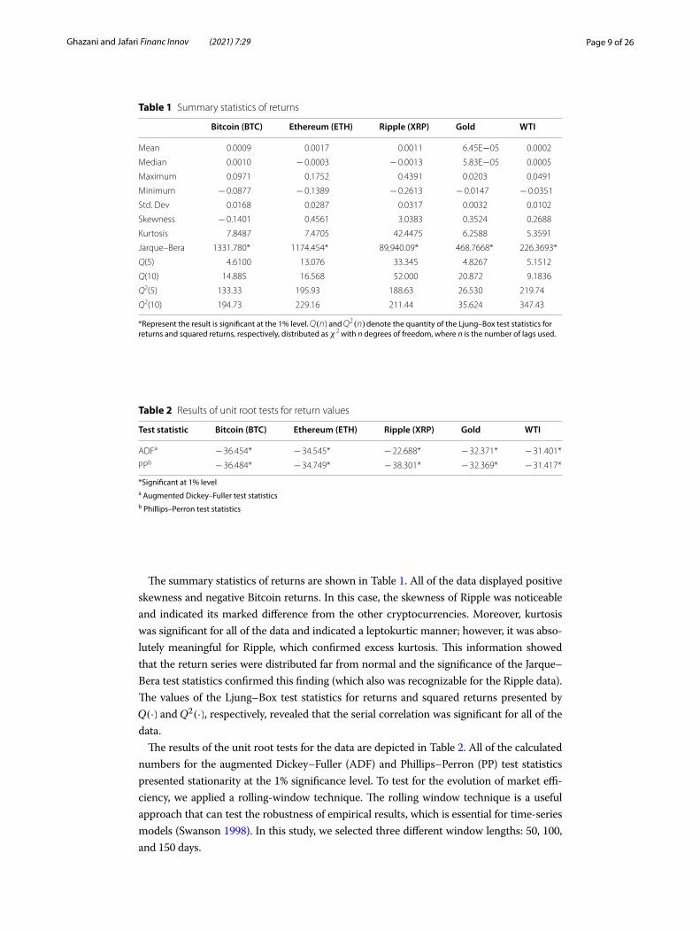
Accordingly, the following figures show each of the variables’ behaviors in terms of market efficiency. Figure 1 expresses the variation in the number of observations,3 and the results showed the market’s inefficiency. As the figure reveals, some data, such as Bitcoin, Ripple, and WTI, moved along with the increasing window length toward an improved market efficiency situation. This phenomenon was evident in Bitcoin. For the other data (including Ethereum and gold), we found a declining trend in market effi-ciency, which was specifically noticeable as the study’s time window increased from 100 to 150 days.

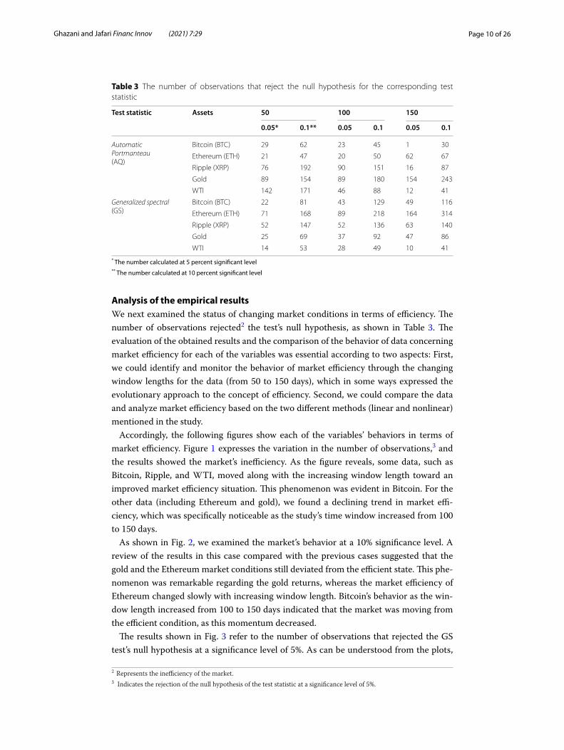
As shown in Fig. 2, we examined the market’s behavior at a 10% significance level. A review of the results in this case compared with the previous cases suggested that the gold and the Ethereum market conditions still deviated from the efficient state. This phe-nomenon was remarkable regarding the gold returns, whereas the market efficiency of Ethereum changed slowly with increasing window length. Bitcoin’s behavior as the win-dow length increased from 100 to 150 days indicated that the market was moving from the efficient condition, as this momentum decreased.

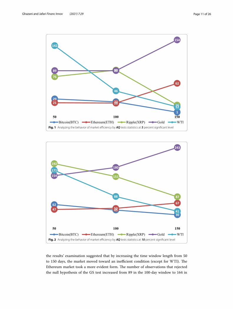
The results shown in Fig. 3 refer to the number of observations that rejected the GS test’s null hypothesis at a significance level of 5%. As can be understood from the plots,

Table 3 The number of observations that reject the null hypothesis for the corresponding test statistic

* The number calculated at 5 percent significant level** The number calculated at 10 percent significant level

Test statistic Assets 50 100 150

0.05* 0.1** 0.05 0.1 0.05 0.1

AutomaticPortmanteau(AQ)

Bitcoin (BTC) 29 62 23 45 1 30

Ethereum (ETH) 21 47 20 50 62 67

Ripple (XRP) 76 192 90 151 16 87

Gold 89 154 89 180 154 243

WTI 142 171 46 88 12 41

Generalized spectral(GS)

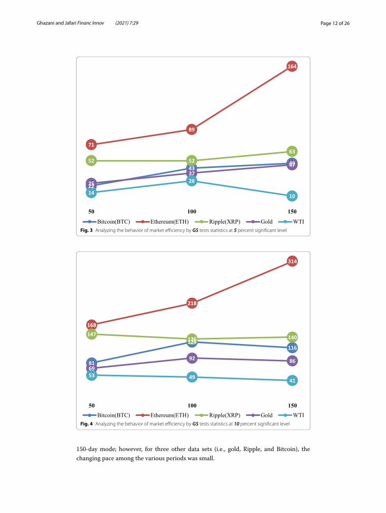
Bitcoin (BTC) 22 81 43 129 49 116

Ethereum (ETH) 71 168 89 218 164 314

Ripple (XRP) 52 147 52 136 63 140

Gold 25 69 37 92 47 86

WTI 14 53 28 49 10 41

2 Represents the inefficiency of the market.3 Indicates the rejection of the null hypothesis of the test statistic at a significance level of 5%.


the results’ examination suggested that by increasing the time window length from 50 to 150 days, the market moved toward an inefficient condition (except for WTI). The Ethereum market took a more evident form. The number of observations that rejected the null hypothesis of the GS test increased from 89 in the 100-day window to 164 in

2923

1

21 20

62

76

90

16

89 89

154142

46

12

50 100 150Bitcoin(BTC) Ethereum(ETH) Ripple(XRP) Gold WTI

Fig. 1 Analyzing the behavior of market efficiency by AQ tests statistics at 5 percent significant level

6245

3047 50

67

192

151

87

154

180

243

171

88

41

50 100 150

Bitcoin(BTC) Ethereum(ETH) Ripple(XRP) Gold WTIFig. 2 Analyzing the behavior of market efficiency by AQ tests statistics at 10 percent significant level


150-day mode; however, for three other data sets (i.e., gold, Ripple, and Bitcoin), the changing pace among the various periods was small.

22

4349

71

89

164

52 5263

25

3747

14

28

10

50 100 150

Bitcoin(BTC) Ethereum(ETH) Ripple(XRP) Gold WTIFig. 3 Analyzing the behavior of market efficiency by GS tests statistics at 5 percent significant level

81

129116

168

218

314

147136 140

69

92 86

53 49 41

50 100 150Bitcoin(BTC) Ethereum(ETH) Ripple(XRP) Gold WTI

Fig. 4 Analyzing the behavior of market efficiency by GS tests statistics at 10 percent significant level


Figure 4 illustrates the GS test’s relevant results at a significance level of 10%. The behavior of the market varied over two different periods (50–100 and 100–150 days) and pertained to two series of data (gold and Bitcoin). Therefore, in the period from 50 to 100 days, we found the related market distances from the efficient condition. With an increase in the time window from 100 to 150 days, however, the situation slightly improved. Ethereum, in this case, as before, also encountered a reduction in its market efficiency.

Analysis of the evolving behavior of market efficiency

This section evaluated the study results based on the two different methods (AQ and GS test statistics). The results were investigated in various time windows (50–150 days) to measure the degree of conformity of these results with the AMH. Additionally, by comparing the results of each study’s data, we can better understand the relevance of the relationship between markets and their alignment. The evolutionary behavior of the data with respect to market efficiency and in different periods has been studied based on this idea. We first analyzed the results based on the AQ method.

Evaluation of the results based on the AQ method

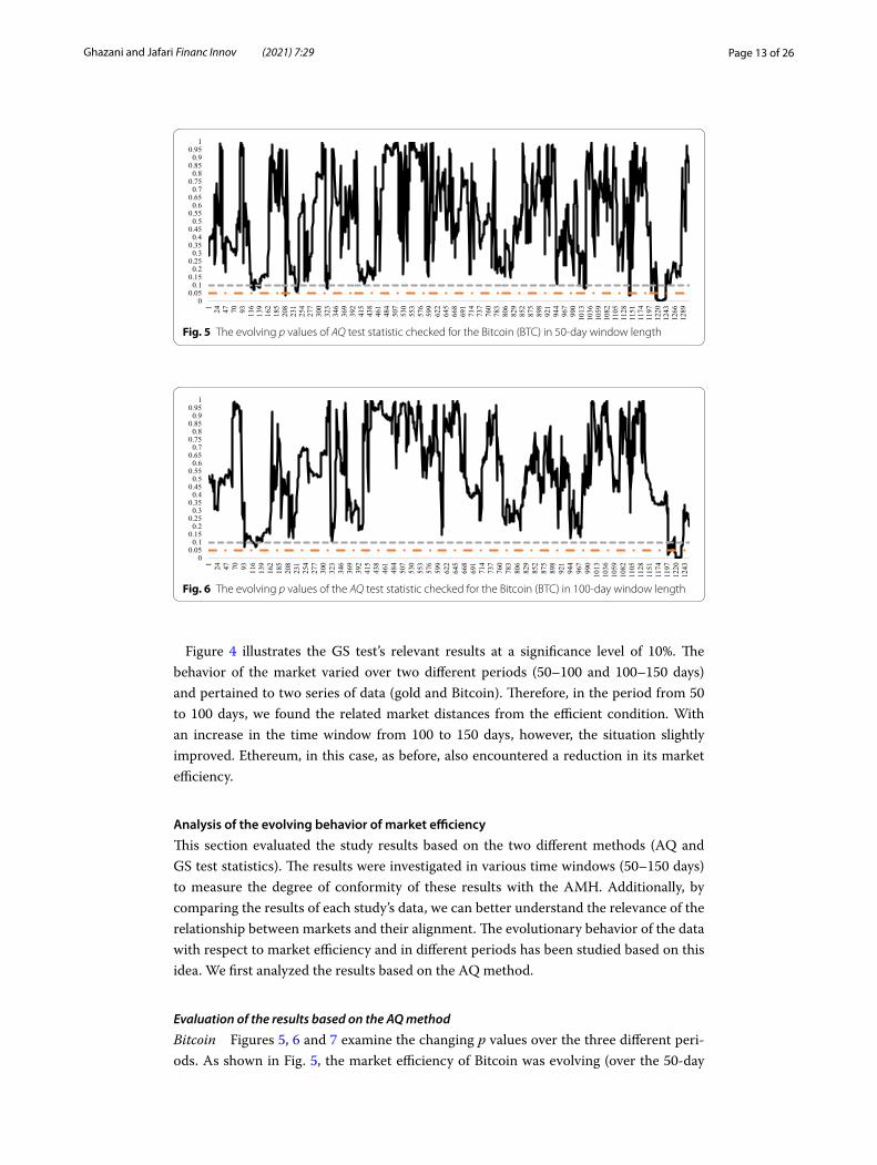
Bitcoin Figures 5, 6 and 7 examine the changing p values over the three different peri-ods. As shown in Fig. 5, the market efficiency of Bitcoin was evolving (over the 50-day

00.050.10.150.20.250.30.350.40.450.50.550.60.650.70.750.80.850.90.95

1

1 24 47 70 93 116

139

162

185

208

231

254

277

300

323

346

369

392

415

438

461

484

507

530

553

576

599

622

645

668

691

714

737

760

783

806

829

852

875

898

921

944

967

990

1013

1036

1059

1082

1105

1128

1151

1174

1197

1220

1243

1266

1289

Fig. 5 The evolving p values of AQ test statistic checked for the Bitcoin (BTC) in 50-day window length

00.050.1

0.150.2

0.250.3

0.350.4

0.450.5

0.550.6

0.650.7

0.750.8

0.850.9

0.951

1 24 47 70 93 116

139

162

185

208

231

254

277

300

323

346

369

392

415

438

461

484

507

530

553

576

599

622

645

668

691

714

737

760

783

806

829

852

875

898

921

944

967

990

1013

1036

1059

1082

1105

1128

1151

1174

1197

1220

1243

Fig. 6 The evolving p values of the AQ test statistic checked for the Bitcoin (BTC) in 100-day window length


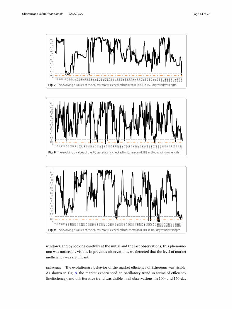
window), and by looking carefully at the initial and the last observations, this phenome-non was noticeably visible. In previous observations, we detected that the level of market inefficiency was significant.

Ethereum The evolutionary behavior of the market efficiency of Ethereum was visible. As shown in Fig. 8, the market experienced an oscillatory trend in terms of efficiency (inefficiency), and this iterative trend was visible in all observations. In 100- and 150-day

00.050.1

0.150.2

0.250.3

0.350.4

0.450.5

0.550.6

0.650.7

0.750.8

0.850.9

0.951

1 20 39 58 77 96 115

134

153

172

191

210

229

248

267

286

305

324

343

362

381

400

419

438

457

476

495

514

533

552

571

590

609

628

647

666

685

704

723

742

761

780

799

818

837

856

875

894

913

932

951

970

989

1008

1027

1046

1065

1084

1103

1122

1141

1160

1179

1198

Fig. 7 The evolving p values of the AQ test statistic checked for Bitcoin (BTC) in 150-day window length

00.050.1

0.150.2

0.250.3

0.350.4

0.450.5

0.550.6

0.650.7

0.750.8

0.850.9

0.951

1 24 47 70 93 116

139

162

185

208

231

254

277

300

323

346

369

392

415

438

461

484

507

530

553

576

599

622

645

668

691

714

737

760

783

806

829

852

875

898

921

944

967

990

1013

1036

1059

1082

1105

1128

1151

1174

1197

1220

1243

1266

1289

Fig. 8 The evolving p values of the AQ test statistic checked for Ethereum (ETH) in 50-day window length

00.050.1

0.150.2

0.250.3

0.350.4

0.450.5

0.550.6

0.650.7

0.750.8

0.850.9

0.951

1 23 45 67 89 111

133

155

177

199

221

243

265

287

309

331

353

375

397

419

441

463

485

507

529

551

573

595

617

639

661

683

705

727

749

771

793

815

837

859

881

903

925

947

969

991

1013

1035

1057

1079

1101

1123

1145

1167

1189

1211

1233

Fig. 9 The evolving p values of the AQ test statistic checked for Ethereum (ETH) in 100-day window length


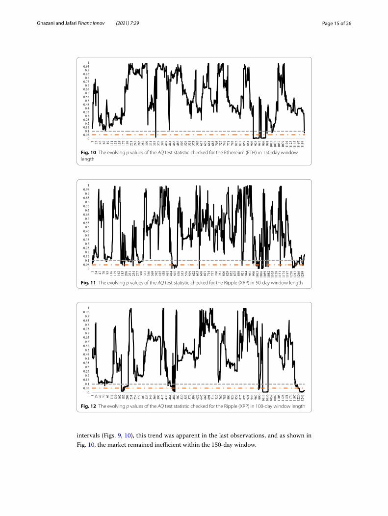
intervals (Figs. 9, 10), this trend was apparent in the last observations, and as shown in Fig. 10, the market remained inefficient within the 150-day window.

00.050.1

0.150.2

0.250.3

0.350.4

0.450.5

0.550.6

0.650.7

0.750.8

0.850.9

0.951

1 23 45 67 89 111

133

155

177

199

221

243

265

287

309

331

353

375

397

419

441

463

485

507

529

551

573

595

617

639

661

683

705

727

749

771

793

815

837

859

881

903

925

947

969

991

1013

1035

1057

1079

1101

1123

1145

1167

1189

Fig. 10 The evolving p values of the AQ test statistic checked for the Ethereum (ETH) in 150-day window length

00.050.1

0.150.2

0.250.3

0.350.4

0.450.5

0.550.6

0.650.7

0.750.8

0.850.9

0.951

1 24 47 70 93 116

139

162

185

208

231

254

277

300

323

346

369

392

415

438

461

484

507

530

553

576

599

622

645

668

691

714

737

760

783

806

829

852

875

898

921

944

967

990

1013

1036

1059

1082

1105

1128

1151

1174

1197

1220

1243

1266

1289

Fig. 11 The evolving p values of the AQ test statistic checked for the Ripple (XRP) in 50-day window length

00.050.1

0.150.2

0.250.3

0.350.4

0.450.5

0.550.6

0.650.7

0.750.8

0.850.9

0.951

1 24 47 70 93 116

139

162

185

208

231

254

277

300

323

346

369

392

415

438

461

484

507

530

553

576

599

622

645

668

691

714

737

760

783

806

829

852

875

898

921

944

967

990

1013

1036

1059

1082

1105

1128

1151

1174

1197

1220

1243



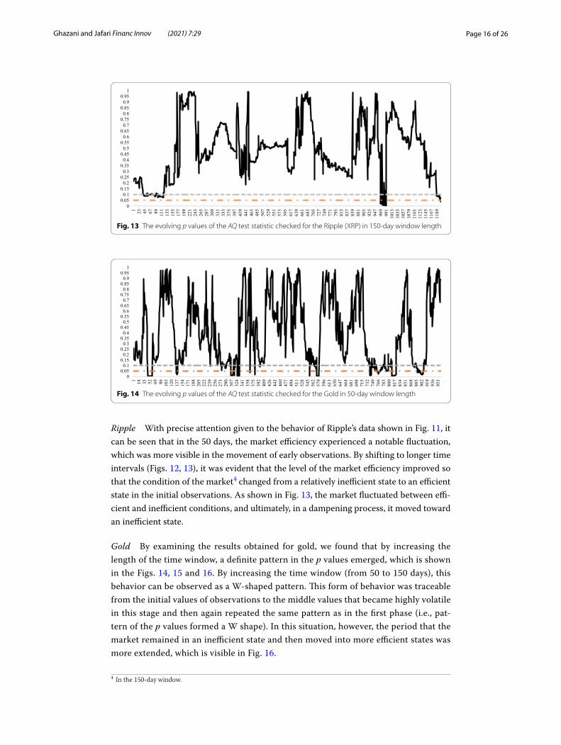
Ripple With precise attention given to the behavior of Ripple’s data shown in Fig. 11, it can be seen that in the 50 days, the market efficiency experienced a notable fluctuation, which was more visible in the movement of early observations. By shifting to longer time intervals (Figs. 12, 13), it was evident that the level of the market efficiency improved so that the condition of the market4 changed from a relatively inefficient state to an efficient state in the initial observations. As shown in Fig. 13, the market fluctuated between effi-cient and inefficient conditions, and ultimately, in a dampening process, it moved toward an inefficient state.

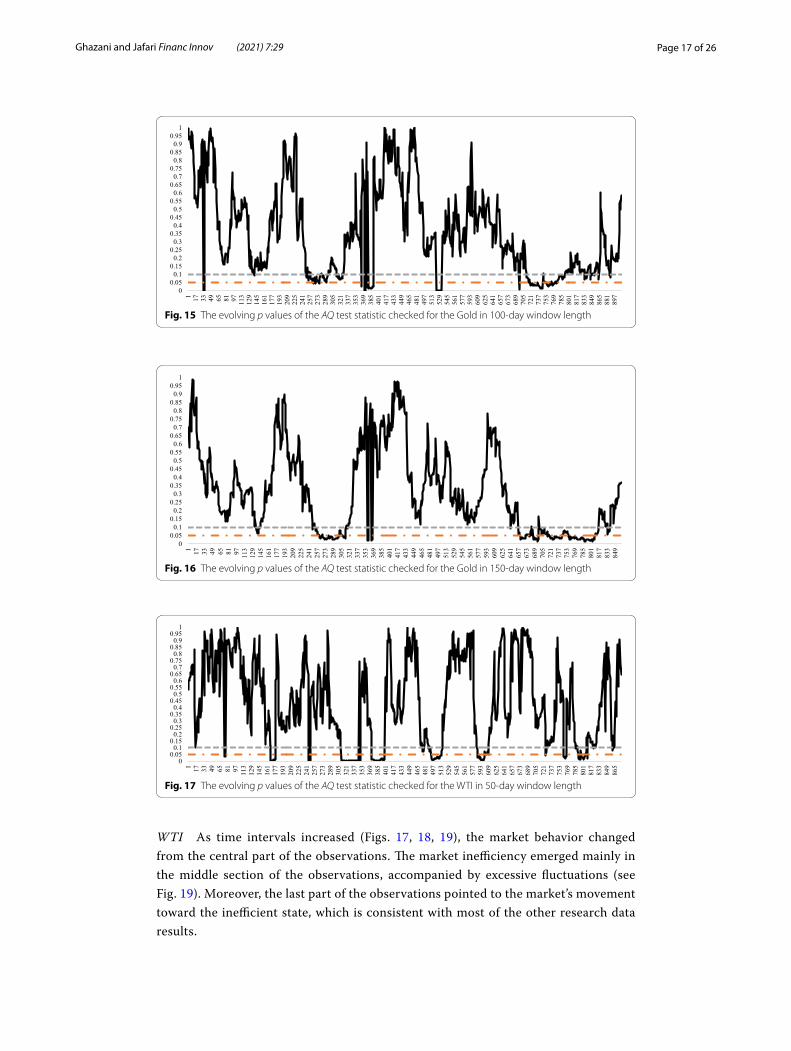
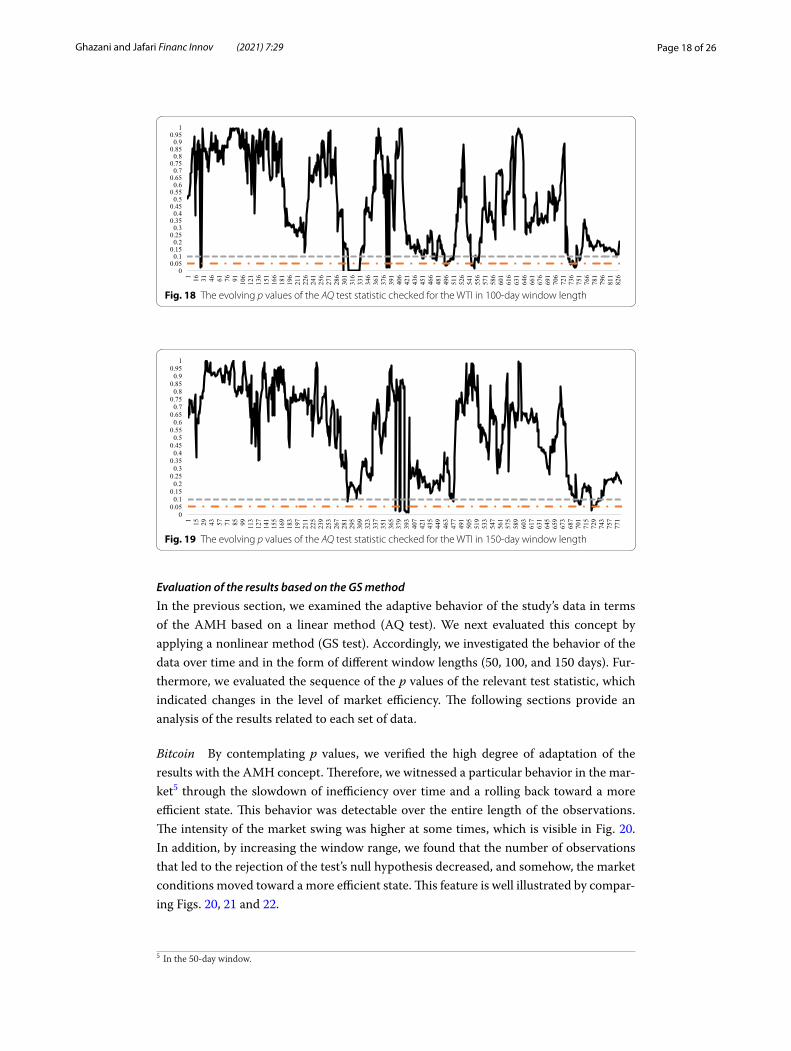
Gold By examining the results obtained for gold, we found that by increasing the length of the time window, a definite pattern in the p values emerged, which is shown in the Figs. 14, 15 and 16. By increasing the time window (from 50 to 150 days), this behavior can be observed as a W-shaped pattern. This form of behavior was traceable from the initial values of observations to the middle values that became highly volatile in this stage and then again repeated the same pattern as in the first phase (i.e., pat-tern of the p values formed a W shape). In this situation, however, the period that the market remained in an inefficient state and then moved into more efficient states was more extended, which is visible in Fig. 16.

00.050.1

0.150.2

0.250.3

0.350.4

0.450.5

0.550.6

0.650.7

0.750.8

0.850.9

0.951

1 23 45 67 89 111

133

155

177

199

221

243

265

287

309

331

353

375

397

419

441

463

485

507

529

551

573

595

617

639

661

683

705

727

749

771

793

815

837

859

881

903

925

947

969

991

1013

1035

1057

1079

1101

1123

1145

1167

1189


00.050.1

0.150.2

0.250.3

0.350.4

0.450.5

0.550.6

0.650.7

0.750.8

0.850.9

0.951

1 18 35 52 69 86 103

120

137

154

171

188

205

222

239

256

273

290

307

324

341

358

375

392

409

426

443

460

477

494

511

528

545

562

579

596

613

630

647

664

681

698

715

732

749

766

783

800

817

834

851

868

885

902

919

936

953

Fig. 14 The evolving p values of the AQ test statistic checked for the Gold in 50-day window length

4 In the 150-day window.


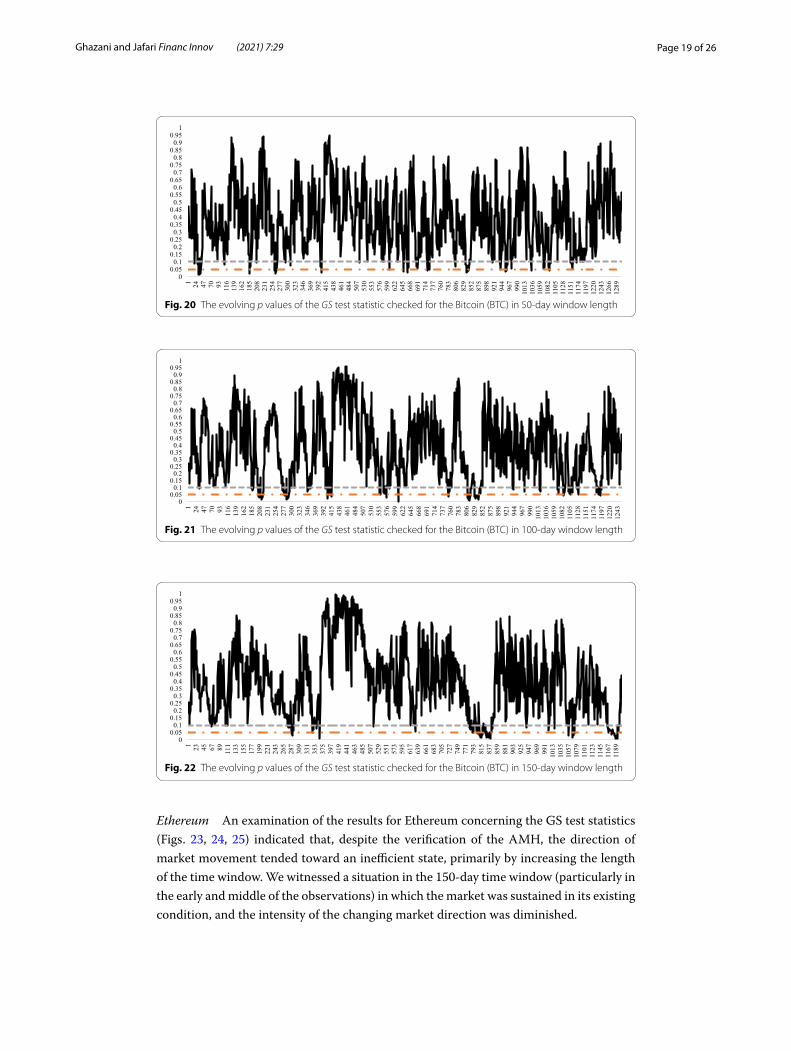
WTI As time intervals increased (Figs. 17, 18, 19), the market behavior changed from the central part of the observations. The market inefficiency emerged mainly in the middle section of the observations, accompanied by excessive fluctuations (see Fig. 19). Moreover, the last part of the observations pointed to the market’s movement toward the inefficient state, which is consistent with most of the other research data results.

00.050.1

0.150.2

0.250.3

0.350.4

0.450.5

0.550.6

0.650.7

0.750.8

0.850.9

0.951

1 17 33 49 65 81 97 113

129

145

161

177

193

209

225

241

257

273

289

305

321

337

353

369

385

401

417

433

449

465

481

497

513

529

545

561

577

593

609

625

641

657

673

689

705

721

737

753

769

785

801

817

833

849

865

881

897


00.050.1

0.150.2

0.250.3

0.350.4

0.450.5

0.550.6

0.650.7

0.750.8

0.850.9

0.951

1 17 33 49 65 81 97 113

129

145

161

177

193

209

225

241

257

273

289

305

321

337

353

369

385

401

417

433

449

465

481

497

513

529

545

561

577

593

609

625

641

657

673

689

705

721

737

753

769

785

801

817

833

849


00.050.1

0.150.2

0.250.3

0.350.4

0.450.5

0.550.6

0.650.7

0.750.8

0.850.9

0.951

1 17 33 49 65 81 97 113

129

145

161

177

193

209

225

241

257

273

289

305

321

337

353

369

385

401

417

433

449

465

481

497

513

529

545

561

577

593

609

625

641

657

673

689

705

721

737

753

769

785

801

817

833

849

865

Fig. 17 The evolving p values of the AQ test statistic checked for the WTI in 50-day window length


Evaluation of the results based on the GS method

In the previous section, we examined the adaptive behavior of the study’s data in terms of the AMH based on a linear method (AQ test). We next evaluated this concept by applying a nonlinear method (GS test). Accordingly, we investigated the behavior of the data over time and in the form of different window lengths (50, 100, and 150 days). Fur-thermore, we evaluated the sequence of the p values of the relevant test statistic, which indicated changes in the level of market efficiency. The following sections provide an analysis of the results related to each set of data.

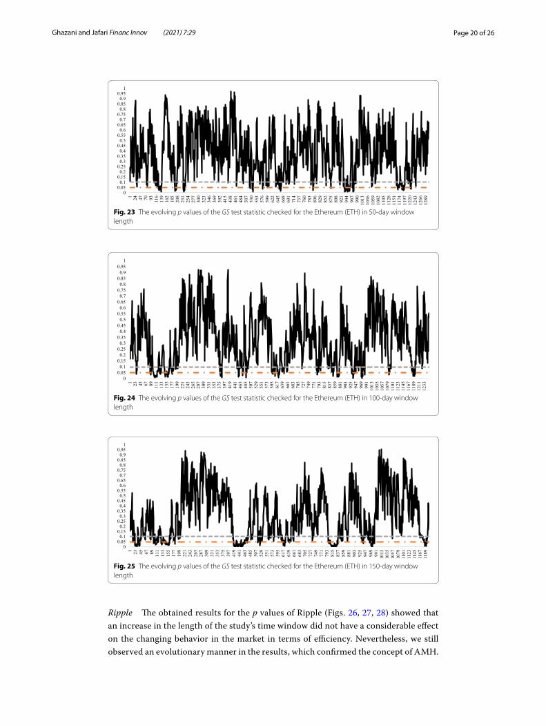
Bitcoin By contemplating p values, we verified the high degree of adaptation of the results with the AMH concept. Therefore, we witnessed a particular behavior in the mar-ket5 through the slowdown of inefficiency over time and a rolling back toward a more efficient state. This behavior was detectable over the entire length of the observations. The intensity of the market swing was higher at some times, which is visible in Fig. 20. In addition, by increasing the window range, we found that the number of observations that led to the rejection of the test’s null hypothesis decreased, and somehow, the market conditions moved toward a more efficient state. This feature is well illustrated by compar-ing Figs. 20, 21 and 22.

00.050.1

0.150.2

0.250.3

0.350.4

0.450.5

0.550.6

0.650.7

0.750.8

0.850.9

0.951

1 16 31 46 61 76 91 106

121

136

151

166

181

196

211

226

241

256

271

286

301

316

331

346

361

376

391

406

421

436

451

466

481

496

511

526

541

556

571

586

601

616

631

646

661

676

691

706

721

736

751

766

781

796

811

826


00.050.1

0.150.2

0.250.3

0.350.4

0.450.5

0.550.6

0.650.7

0.750.8

0.850.9

0.951

1 15 29 43 57 71 85 99 113

127

141

155

169

183

197

211

225

239

253

267

281

295

309

323

337

351

365

379

393

407

421

435

449

463

477

491

505

519

533

547

561

575

589

603

617

631

645

659

673

687

701

715

729

743

757

771


5 In the 50-day window.


Ethereum An examination of the results for Ethereum concerning the GS test statistics (Figs. 23, 24, 25) indicated that, despite the verification of the AMH, the direction of market movement tended toward an inefficient state, primarily by increasing the length of the time window. We witnessed a situation in the 150-day time window (particularly in the early and middle of the observations) in which the market was sustained in its existing condition, and the intensity of the changing market direction was diminished.

00.050.1

0.150.2

0.250.3

0.350.4

0.450.5

0.550.6

0.650.7

0.750.8

0.850.9

0.951

1 24 47 70 93 116

139

162

185

208

231

254

277

300

323

346

369

392

415

438

461

484

507

530

553

576

599

622

645

668

691

714

737

760

783

806

829

852

875

898

921

944

967

990

1013

1036

1059

1082

1105

1128

1151

1174

1197

1220

1243

1266

1289

Fig. 20 The evolving p values of the GS test statistic checked for the Bitcoin (BTC) in 50-day window length

00.050.1

0.150.2

0.250.3

0.350.4

0.450.5

0.550.6

0.650.7

0.750.8

0.850.9

0.951

1 24 47 70 93 116

139

162

185

208

231

254

277

300

323

346

369

392

415

438

461

484

507

530

553

576

599

622

645

668

691

714

737

760

783

806

829

852

875

898

921

944

967

990

1013

1036

1059

1082

1105

1128

1151

1174

1197

1220

1243


00.050.1

0.150.2

0.250.3

0.350.4

0.450.5

0.550.6

0.650.7

0.750.8

0.850.9

0.951

1 23 45 67 89 111

133

155

177

199

221

243

265

287

309

331

353

375

397

419

441

463

485

507

529

551

573

595

617

639

661

683

705

727

749

771

793

815

837

859

881

903

925

947

969

991

1013

1035

1057

1079

1101

1123

1145

1167

1189



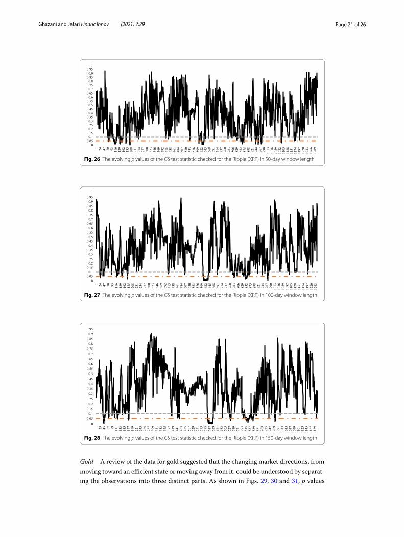
Ripple The obtained results for the p values of Ripple (Figs. 26, 27, 28) showed that an increase in the length of the study’s time window did not have a considerable effect on the changing behavior in the market in terms of efficiency. Nevertheless, we still observed an evolutionary manner in the results, which confirmed the concept of AMH.

00.050.1

0.150.2

0.250.3

0.350.4

0.450.5

0.550.6

0.650.7

0.750.8

0.850.9

0.951

1 24 47 70 93 116

139

162

185

208

231

254

277

300

323

346

369

392

415

438

461

484

507

530

553

576

599

622

645

668

691

714

737

760

783

806

829

852

875

898

921

944

967

990

1013

1036

1059

1082

1105

1128

1151

1174

1197

1220

1243

1266

1289

Fig. 23 The evolving p values of the GS test statistic checked for the Ethereum (ETH) in 50-day window length

00.050.1

0.150.2

0.250.3

0.350.4

0.450.5

0.550.6

0.650.7

0.750.8

0.850.9

0.951

1 23 45 67 89 111

133

155

177

199

221

243

265

287

309

331

353

375

397

419

441

463

485

507

529

551

573

595

617

639

661

683

705

727

749

771

793

815

837

859

881

903

925

947

969

991

1013

1035

1057

1079

1101

1123

1145

1167

1189

1211

1233


00.050.1

0.150.2

0.250.3

0.350.4

0.450.5

0.550.6

0.650.7

0.750.8

0.850.9

0.951

1 23 45 67 89 111

133

155

177

199

221

243

265

287

309

331

353

375

397

419

441

463

485

507

529

551

573

595

617

639

661

683

705

727

749

771

793

815

837

859

881

903

925

947

969

991

1013

1035

1057

1079

1101

1123

1145

1167

1189



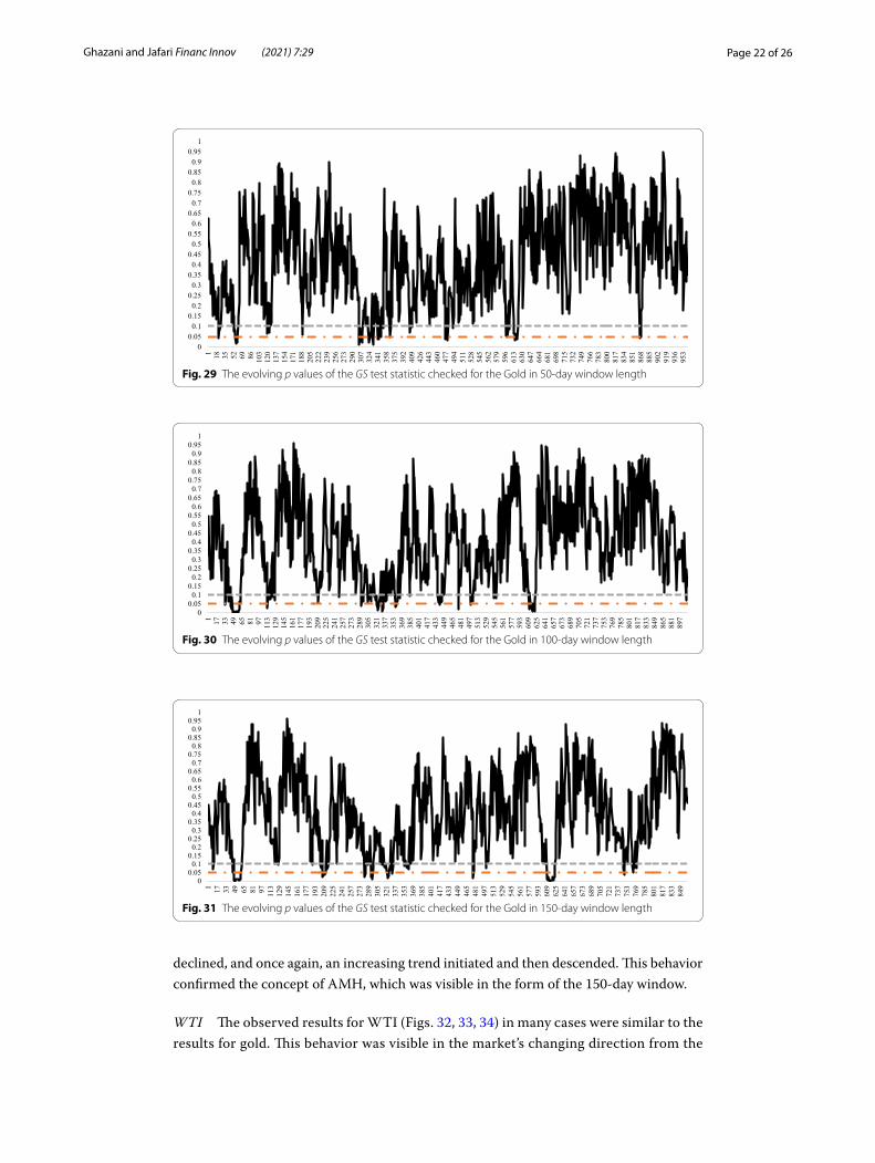
Gold A review of the data for gold suggested that the changing market directions, from moving toward an efficient state or moving away from it, could be understood by separat-ing the observations into three distinct parts. As shown in Figs. 29, 30 and 31, p values

00.050.1

0.150.2

0.250.3

0.350.4

0.450.5

0.550.6

0.650.7

0.750.8

0.850.9

0.951

1 24 47 70 93 116

139

162

185

208

231

254

277

300

323

346

369

392

415

438

461

484

507

530

553

576

599

622

645

668

691

714

737

760

783

806

829

852

875

898

921

944

967

990

1013

1036

1059

1082

1105

1128

1151

1174

1197

1220

1243

1266

1289

Fig. 26 The evolving p values of the GS test statistic checked for the Ripple (XRP) in 50-day window length

00.050.1

0.150.2

0.250.3

0.350.4

0.450.5

0.550.6

0.650.7

0.750.8

0.850.9

0.951

1 24 47 70 93 116

139

162

185

208

231

254

277

300

323

346

369

392

415

438

461

484

507

530

553

576

599

622

645

668

691

714

737

760

783

806

829

852

875

898

921

944

967

990

1013

1036

1059

1082

1105

1128

1151

1174

1197

1220

1243


00.050.1

0.150.2

0.250.3

0.350.4

0.450.5

0.550.6

0.650.7

0.750.8

0.850.9

0.95

1 23 45 67 89 111

133

155

177

199

221

243

265

287

309

331

353

375

397

419

441

463

485

507

529

551

573

595

617

639

661

683

705

727

749

771

793

815

837

859

881

903

925

947

969

991

1013

1035

1057

1079

1101

1123

1145

1167

1189



declined, and once again, an increasing trend initiated and then descended. This behavior confirmed the concept of AMH, which was visible in the form of the 150-day window.

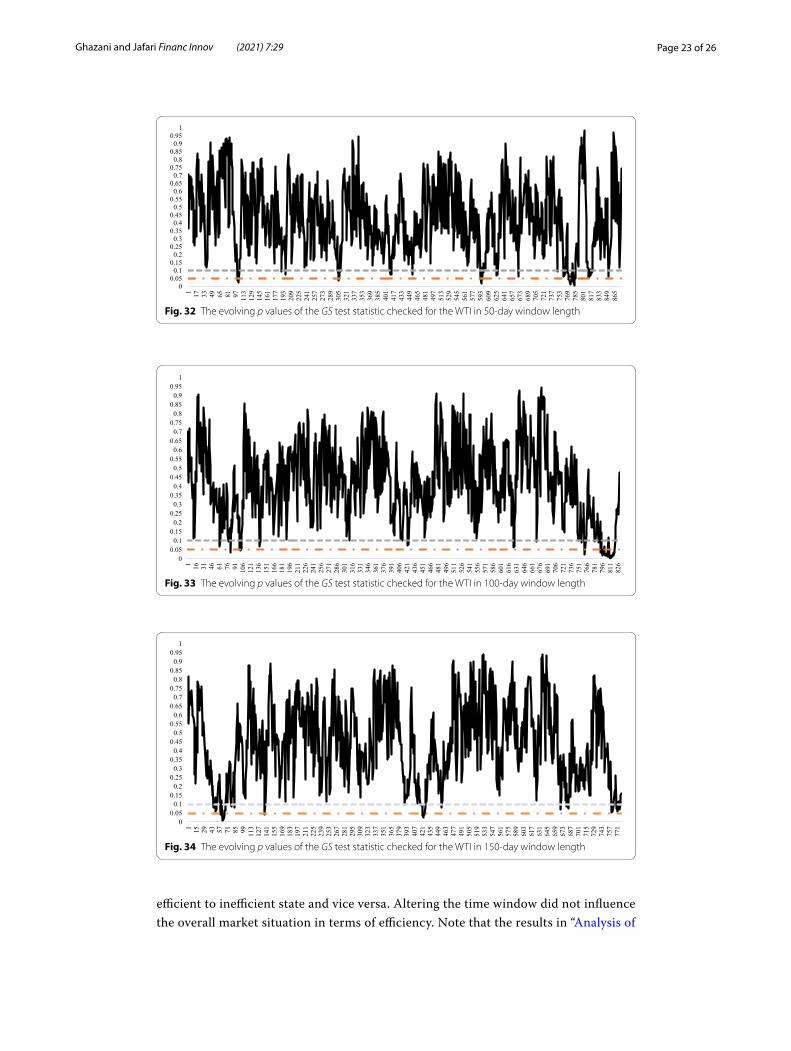
WTI The observed results for WTI (Figs. 32, 33, 34) in many cases were similar to the results for gold. This behavior was visible in the market’s changing direction from the

00.050.1

0.150.2

0.250.3

0.350.4

0.450.5

0.550.6

0.650.7

0.750.8

0.850.9

0.951

1 18 35 52 69 86 103

120

137

154

171

188

205

222

239

256

273

290

307

324

341

358

375

392

409

426

443

460

477

494

511

528

545

562

579

596

613

630

647

664

681

698

715

732

749

766

783

800

817

834

851

868

885

902

919

936

953

Fig. 29 The evolving p values of the GS test statistic checked for the Gold in 50-day window length

00.050.1

0.150.2

0.250.3

0.350.4

0.450.5

0.550.6

0.650.7

0.750.8

0.850.9

0.951

1 17 33 49 65 81 97 113

129

145

161

177

193

209

225

241

257

273

289

305

321

337

353

369

385

401

417

433

449

465

481

497

513

529

545

561

577

593

609

625

641

657

673

689

705

721

737

753

769

785

801

817

833

849

865

881

897


00.050.1

0.150.2

0.250.3

0.350.4

0.450.5

0.550.6

0.650.7

0.750.8

0.850.9

0.951

1 17 33 49 65 81 97 113

129

145

161

177

193

209

225

241

257

273

289

305

321

337

353

369

385

401

417

433

449

465

481

497

513

529

545

561

577

593

609

625

641

657

673

689

705

721

737

753

769

785

801

817

833

849



efficient to inefficient state and vice versa. Altering the time window did not influence the overall market situation in terms of efficiency. Note that the results in “Analysis of

00.050.1

0.150.2

0.250.3

0.350.4

0.450.5

0.550.6

0.650.7

0.750.8

0.850.9

0.951

1 17 33 49 65 81 97 113

129

145

161

177

193

209

225

241

257

273

289

305

321

337

353

369

385

401

417

433

449

465

481

497

513

529

545

561

577

593

609

625

641

657

673

689

705

721

737

753

769

785

801

817

833

849

865

Fig. 32 The evolving p values of the GS test statistic checked for the WTI in 50-day window length

00.050.1

0.150.2

0.250.3

0.350.4

0.450.5

0.550.6

0.650.7

0.750.8

0.850.9

0.951

1 16 31 46 61 76 91 106

121

136

151

166

181

196

211

226

241

256

271

286

301

316

331

346

361

376

391

406

421

436

451

466

481

496

511

526

541

556

571

586

601

616

631

646

661

676

691

706

721

736

751

766

781

796

811

826


00.050.1

0.150.2

0.250.3

0.350.4

0.450.5

0.550.6

0.650.7

0.750.8

0.850.9

0.951

1 15 29 43 57 71 85 99 113

127

141

155

169

183

197

211

225

239

253

267

281

295

309

323

337

351

365

379

393

407

421

435

449

463

477

491

505

519

533

547

561

575

589

603

617

631

645

659

673

687

701

715

729

743

757

771



the empirical results” section, in which the number of p values that rejected the null hypothesis was computed, confirmed this finding.

ConclusionThis study scrutinized the evolving efficiency by utilizing daily historical data for the three benchmark cryptocurrencies (Bitcoin, Ethereum, and Ripple), gold, and WTI crude oil. To assess any variation in market efficiency and check the market’s evolv-ing behavior over time, we applied a rolling-sample technique with diverse window lengths that was consistent with AMH implications. We applied two alternative tests to examine linear and nonlinear dependency, which included AQ and GS. We ana-lyzed the obtained results from two aspects: First, we focused on each market’s over-all condition in terms of efficiency and degree of conformity with the AMH. Second, we examined the evolving behavior of each market by moving toward longer window lengths (e.g., from 50 to 150 days).

Considering these results, the observed behavior in all markets indicated verifica-tion of the AMH, but the degree of adaptability of the data was different. According to the AQ test statistic, which was a linear method, we observed that the degree of adaptation of Bitcoin with respect to the AMH concept was relatively trivial (in other words, the change in market direction from an efficient state to an inefficient state and vice versa was insignificant). Gold returns, however, represented a greater degree of conformity with the AMH. Furthermore, concerning the achieved results of the GS test, which was a nonlinear method, we found that the level of adaptability of WTI with AMH was relatively insignificant. In contrast, Ethereum showed a more compat-ible manner from an evolutionary perspective with respect to market efficiency.

Another aspect of the study was to analyze the existence of evolutionary behavior in the market. To achieve this goal, we checked the results by applying a rolling-win-dow method with three different window lengths (50, 100, and 150 days) to the test statistics. When we increased the window length for each set of data, the market’s behavior (in terms of efficiency) changed. For example, at a significance level of 10% and based on the AQ test, the market efficiency of Ethereum improved slowly as the window length increased. For the GS test results at the same level of significance, we found that the market changed over two different periods (from 50 to 100 and 100 to 150 days) for gold and Bitcoin. Thus, in the period of 50–100 days, we observed mar-ket distances during the efficient conditions; however, as the window length increased from 100 to 150 days, the situation improved slightly.

AbbreviationsAQ: Automatic portmanteau; GS: Generalized spectral; AMH: Adaptive market hypothesis; EMH: Efficient Market hypoth-esis; MDH: Martingale difference hypothesis; AIC: Akaike information criterion; BIC: Bayesian information criterion; ADF: Augmented Dickey–Fuller; PP: Phillips–Perron.

AcknowledgementsNot applicable.

Authors’ contributionsMMG: Conceptualization, investigation, methodology, formal analysis, visualization, writing the original draft; MAJ: Cal-culation, review, editing and made suggestions to improve the quality of the manuscript. All authors read and approved the final manuscript.


FundingThe authors declare that this research received no specific financial support from any funding agency in the public, com-mercial, or not-for-profit sectors.

Availability of data and materialsThe datasets used and/or analyzed during the current study are available upon request.

Declarations

Competing interestsThe authors declare that they have no competing interests.

Received: 23 July 2020 Accepted: 19 April 2021

ReferencesBariviera AF (2017) The inefficiency of Bitcoin revisited: A dynamic approach. Econ Lett 161:1–4Baur DG, Dimpfl T, Jung RC (2012) Stock return autocorrelations revisited: a quantile regression approach. J Empir Financ

19(2):254–265Borges MR (2010) Efficient market hypothesis in European stock markets. Eur J Finance 16(7):711–726Bouri E, Georges A, Anne Haubo D (2016) On the Return-volatility Relationship in the Bitcoin Market around the Price

Crash of 2013. Economics Discussion Papers, No 2016-41. Kiel Institute for the World Economy. http:// www. Econo mics- ejour nal. org/ econo mics/ discu ssion papers/2016-41.

Campbell JY, Champbell JJ, Campbell JW, Lo AW, Lo AWC, MacKinlay AC (1997) The econometrics of financial markets. Princeton University Press

Caporale GM, Gil-Alana L, Plastun A, Makarenko I (2016) Long memory in the Ukrainian stock market and financial crises. J Econ Finance 40(2):235–257

Caporale GM, Gil-Alana L, Plastun A (2018) Persistence in the cryptocurrency market. Res Int Bus Financ 46:141–148Chao X, Kou G, Peng Y, Alsaadi FE (2019) Behavior monitoring methods for trade-based money laundering integrating

macro and micro prudential regulation: a case from China. Technol Econ Dev Econ 25(6):1081–1096Charles A, Darné O, Kim JH (2012) Exchange-rate return predictability and the adaptive markets hypothesis: evidence

from major foreign exchange rates. J Int Money Financ 31(6):1607–1626Chen H, Liu L, Li X (2018) The predictive content of CBOE crude oil volatility index. Phys A 492:837–850Corbet S, Meegan A, Larkin C, Lucey B, Yarovaya L (2018) Exploring the dynamic relationships between cryptocurrencies

and other financial assets. Econ Lett 165:28–34Escanciano JC, Velasco C (2006) Generalized spectral tests for the martingale difference hypothesis. J Econom

134(1):151–185Fama EF, French KR (1988) Permanent and temporary components of stock prices. J Polit Econ 96(2):246–273Farmer JD (2002) Market force, ecology and evolution. Ind Corp Chang 11(5):895–953Farmer JD, Lo AW (1999) Frontiers of finance: Evolution and efficient markets. Proc Natl Acad Sci 96(18):9991–9992Gajardo G, Kristjanpoller WD, Minutolo M (2018) Does Bitcoin exhibit the same asymmetric multifractal cross-correlations

with crude oil, Gold and DJIA as the Euro, Great British Pound and Yen? Chaos Solitons Fractals 109:195–205Ghazani MM, Ebrahimi SB (2019) Testing the adaptive market hypothesis as an evolutionary perspective on market

efficiency: Evidence from the crude oil prices. Financ Res Lett 30:60–68Grossman SJ, Stiglitz JE (1980) On the impossibility of informationally efficient markets. Am Econ Rev 70(3):393–408Hall S, Foxon TJ, Bolton R (2017) Investing in low-carbon transitions: energy finance as an adaptive market. Clim Policy

17(3):280–298Hamilton JD (1996) This is what happened to the oil price-macroeconomy relationship. J Monet Econ 38(2):215–220Jegadeesh N, Titman S (1993) Returns to buying winners and selling losers: Implications for stock market efficiency. J

Finance 48(1):65–91Jin J, Yu J, Hu Y, Shang Y (2019) Which one is more informative in determining price movements of hedging assets?

Evidence from Bitcoin, gold and crude oil markets. Phys A 527:121121Jones CM, Kaul G (1996) Oil and the stock markets. J Financ 51(2):463–491Kang SH, McIver RP, Hernandez JA (2019) Co-movements between Bitcoin and Gold: A wavelet coherence analysis. Phys

A 536:120888Khuntia S, Pattanayak JK (2018) Adaptive market hypothesis and evolving predictability of bitcoin. Econ Lett 167:26–28Kilian L, Park C (2009) The impact of oil price shocks on the US stock market. Int Econ Rev 50(4):1267–1287Kim JH, Shamsuddin A, Lim KP (2011) Stock return predictability and the adaptive markets hypothesis: evidence from

century-long US data. J Empir Financ 18(5):868–879Kou G, Peng Y, Wang G (2014) Evaluation of clustering algorithms for financial risk analysis using MCDM methods. Inf Sci

275:1–12Kou G, Chao X, Peng Y, Alsaadi FE, Herrera-Viedma E (2019) Machine learning methods for systemic risk analysis in finan-

cial sectors. Technol Econ Dev Econ 25(5):716–742Kristoufek L (2018) On Bitcoin markets (in) efficiency and its evolution. Phys A 503:257–262Kristoufek L, Vosvrda M (2013) Measuring capital market efficiency: Global and local correlations structure. Phys A

392(1):184–193Lazăr D, Todea A, Filip D (2012) Martingale difference hypothesis and financial crisis: Empirical evidence from European

emerging foreign exchange markets. Econ Syst 36(3):338–350

http://www.Economics-ejournal.org/economics/discussion

http://www.Economics-ejournal.org/economics/discussion


Le Tran V, Leirvik T (2019) A simple but powerful measure of market efficiency. Finance Res Lett 29:141–151Le Tran V, Leirvik T (2020) Efficiency in the markets of crypto-currencies. Finance Res Lett 35:101382Lei L, Shang Y, Chen Y, Wei Y (2019) Does the financial crisis change the economic risk perception of crude oil traders? A

MIDAS quantile regression approach. Finance Res Lett 30:341–351Lim KP, Brooks R (2011) The evolution of stock market efficiency over time: a survey of the empirical literature. J Econ Surv

25(1):69–108Lo AW (1989) Long-term memory in stock market prices (No. w2984). National Bureau of Economic Research.Lo AW (2004) The adaptive markets hypothesis: Market efficiency from an evolutionary perspective. J Portfolio Manag

(Forthcoming)Lo AW (2005) Reconciling efficient markets with behavioral finance: the adaptive markets hypothesis. J Invest Consult

7(2):21–44Lobato I, Nankervis JC, Savin NE (2001) Testing for autocorrelation using a modified box-pierce Q test. Int Econ Rev

42(1):187–205Nadarajah S, Chu J (2017) On the inefficiency of Bitcoin. Econ Lett 150:6–9Noda A (2016) A test of the adaptive market hypothesis using a time-varying AR model in Japan. Finance Res Lett

17:66–71Noda A (2020) On the evolution of cryptocurrency market efficiency. Appl Econ Lett 1–7.Numapau Gyamfi E (2018) Adaptive market hypothesis: evidence from the Ghanaian stock market. J Afr Bus

19(2):195–209Opong KK, Mulholland G, Fox AF, Farahmand K (1999) The behavior of some UK equity indices: an application of Hurst

and BDS tests. J Empir Financ 6(3):267–282Shahid NM, Mehmood Z (2015) Calendar anomalies in the stock market: A case of KSE 100 index. Int J Afr Asian Stud

7:16–23Simon HA (1955) A behavioral model of rational choice. Q J Econ 69(1):99–118Simon HA (2000) Bounded rationality in social science: today and tomorrow. Mind Soc 1(1):25–39Swanson NR (1998) Money and output viewed through a rolling window. J Monet Econ 41(3):455–474Tang K, Xiong W (2012) Index investment and the financialization of commodities. Finance Anal J 68(6):54–74. https:// doi.

org/ 10. 2469/ faj. v68. n6.5Tripathi A, Vipul V, Dixit A (2020) Adaptive market hypothesis and investor sentiments: global evidence. Manag FinanceUrquhart A (2016) The inefficiency of Bitcoin. Econ Lett 148:80–82Varghese G, Madhavan V (2020) Long memory dynamics and relative efficiency of crude oil benchmarks: An adaptive

market hypothesis perspective. J Affairs. https:// doi. org/ 10. 1002/ pa. 2513Wei WC (2018) Liquidity and market efficiency in cryptocurrencies. Econ Lett 168:21–24Zhang W, Wang P, Li X, Shen D (2018) The inefficiency of cryptocurrency and its cross-correlation with Dow Jones Indus-

trial Average. Phys A 510:658–670

Publisher’s NoteSpringer Nature remains neutral with regard to jurisdictional claims in published maps and institutional affiliations.

https://doi.org/10.2469/faj.v68.n6.5

https://doi.org/10.2469/faj.v68.n6.5

https://doi.org/10.1002/pa.2513

Cryptocurrencies, gold, and WTI crude oil market ...

Documents

Transcript of Cryptocurrencies, gold, and WTI crude oil market ...