©20

10 N

atu

re A

mer

ica,

Inc.

All

rig

hts

res

erve

d.

protocol

nature protocols | VOL.5 NO.10 | 2010 | 1697

IntroDuctIonBiological processes, from cell motility to signal transduction, require large heterogeneous assemblies that undergo dynamic changes. Unfortunately, no single biophysical method yields continuous views of these large biological complexes at atomic resolution. However, single-particle cryo-EM is capable of visualizing these complexes in discrete physiological or bio-chemical states.

It is now relatively common for cryo-EM to achieve subnanom-eter resolutions (reviewed in ref. 1). To date, ~20% of all entries in the EM DataBank (EMDB, http://emdatabank.org/), ranging from ion channels to infectious viruses, have achieved resolutions better than 10 Å. Unfortunately, at resolutions between 5 and 10 Å, atomic models cannot be constructed directly from the cryo-EM density map. However, distinct features in the density map are evident. At subnanometer resolutions, secondary structure elements (SSEs) are visible: α-helices appear as long cylinders, whereas β-sheets appear as thin planes1. Using feature detection and computational geometry algorithms, SSEs can be reliably identified and quanti-fied2,3. The spatial description of SSEs has also been used to infer structure and/or function of individual protein domains, as was done in identifying an annexin-like domain in the HSV-1 major capsid protein4 and the pore structure of RyR1(ref. 5).

Recently, the structure of several biological assemblies have been resolved to better than 4.6 Å resolution with single-particle cryo-EM6–16. In these near-atomic resolution structures, the pitch of α-helices, the separation of β-strands and the densities that connect them can be seen. In these relatively high-resolution structures, many of the bulky side chains can also be seen. However, it should be noted that these structures still do not have the resolution to use standard X-ray crystallographic methods for automatic model construction. In fact, the de novo models built from these structures rely almost entirely on visual interpretation of the density, and on manual structure assignment in cases in which no homologous structures are available9,10,13,16. However, in each of these cases, sig-nificant insight into functional mechanisms and interactions can be reliably obtained from the models; thus providing an excellent framework for future research.

Here, we present our protocol for generating a near-atomic reso-lution cryo-EM density map, analyzing the salient features of the density map and building an atomic model. This protocol has been used in the construction of a complete atomic model for a group II chaperonin from Methanococcus maripaludis (Mm-cpn)14, but is generally applicable to other single-particle specimens imaged with cryo-EM. For instance, the recent 4 Å resolution structure of the chaperonin TRiC/CCT with eight distinct subunits was elucidated with a similar protocol without imposing any symmetry, resolving a longstanding question as to how the eight subunits are arranged in each of the two rings8.

Experimental designThe following protocol is divided into three modules. The first module (Steps 1–13) describes the steps to generate a near-atomic resolution density map from raw two-dimensional (2D) images (Fig. 1). The second module (Steps 14–25) details the procedure for generating a Cα backbone trace directly from the cryo-EM density map (Fig. 2), whereas the third module (Steps 26–33) describes a method for building an atomic model with side chain assignments from the initial Cα backbone trace (Fig. 3).

In the first module, we provide an overview of how the reconstruc-tion of Mm-cpn was achieved at near-atomic resolution. As there are many details and subtleties in approaching a refinement on a new specimen, we suggest running the EMAN17 program and following the four-step tutorial to get more detailed advice for specific projects. This protocol is for EMAN1, which was used for all of our pub-lished structures at the time of writing this paper. EMAN2 (ref. 18) is now available and is easier to use for many of these steps (see Box 1 for further information).

In the second set of steps, we will describe how to construct a model from a near-atomic resolution cryo-EM density map, depending on the availability of known or related atomic mod-els. When a known or related structure for one or more of the components in a macromolecular assembly is known, the model can be fit to the density map and provide initial positioning of atoms in the density map. This requires either previous knowledge

Cryo-EM of macromolecular assemblies at near-atomic resolutionMatthew L Baker1, Junjie Zhang1,2, Steven J Ludtke1 & Wah Chiu1

1National Center for Macromolecular Imaging, Verna and Marrs McLean Department of Biochemistry and Molecular Biology, Baylor College of Medicine, Houston, Texas, USA. 2Present address: Department of Structural Biology, Stanford University, Stanford, California, USA. Correspondence should be addressed to W.C. (wah@bcm.edu).

Published online 30 September 2010; doi:10.1038/nprot.2010.126

With single-particle electron cryomicroscopy (cryo-eM), it is possible to visualize large, macromolecular assemblies in near-native states. although subnanometer resolutions have been routinely achieved for many specimens, state of the art cryo-eM has pushed to near-atomic (3.3–4.6 Å) resolutions. at these resolutions, it is now possible to construct reliable atomic models directly from the cryo-eM density map. In this study, we describe our recently developed protocols for performing the three-dimensional reconstruction and modeling of Mm-cpn, a group II chaperonin, determined to 4.3 Å resolution. this protocol, utilizing the software tools eMan, Gorgon and coot, can be adapted for use with nearly all specimens imaged with cryo-eM that target beyond 5 Å resolution. additionally, the feature recognition and computational modeling tools can be applied to any near-atomic resolution density maps, including those from X-ray crystallography.

©20

10 N

atu

re A

mer

ica,

Inc.

All

rig

hts

res

erve

d.

protocol

1698 | VOL.5 NO.10 | 2010 | nature protocols

or sequence analysis tools to identify structural homologous. Alternatively, if no known or homologous structures are avail-able, the de novo modeling steps (Steps 19–21) can generate an initial Cα backbone model for components of the macro-molecular assembly. If an atomic model is available, Steps 19–21 are not necessary.

In the final set of steps, side chains are added and the entire model is optimized to fit the density while maintaining reason-able geometry. Generally, these steps should only be used when a large percentage of side chains are visible in the density map. Anecdotally, in our 4.2 Å resolution structure of the chaperonin GroEL10, only ~10% of side chain densities were visible and thus a complete model with side chains was not constructed. However, in Mm-cpn, > 65% of side chain densities were observed and thus an entire atomic model could be constructed. Despite similar resolutions, data quality (Mm-cpn images had higher contrast at higher resolution) and differences in the reconstruction steps may have affected the visibility of side chains in GroEL and Mm-cpn. However, the final decision on placement of side chains is at the

EMAN1 (v1.9 or newer) or EMAN2 for 3D reconstruction and data manip-ulations (http://blake.bcm.tmc.edu/eman/); see Box 2 for more information regarding the Image Processing software.Gorgon (v1.0.2 or newer) for initial model building (http://gorgon.wustl.edu/)Coot (v0.6 or newer) for model refinement (http://www.biop.ox.ac.uk/coot/)UCSF Chimera (v1.4 or newer) for map and model visualization (http://www.cgl.ucsf.edu/chimera/)Optional: fitctf.py for automated CTF estimation (requires Matlab (MathWorks); see http://ncmi.bcm.tmc.edu/software/fitctf/doc_html for additional details)

EQUIPMENT SETUPGeneral The steps described in this protocol use several common software packages in cryo-EM and X-ray crystallography. The protocol is modular enough that experienced users may substitute their own software for portions of the model-building procedure. This procedure also assumes that (i) the user has some working knowledge of cryo-EM image processing and density analysis and (ii) the user has a sufficient amount of high-quality homogeneous raw image data acquired from the cryo-EM at resolutions beyond 5 Å based on the visibility of contrast transfer function (CTF) oscillations in the one-dimensional (1D) power spectrum.Digitized micrographs of single particles As previously mentioned, the following protocol will utilize Mm-cpn as an example. A total of 29,926 particles from 616 CCD frames (4k × 4k) were used to produce the 4.3 Å resolution reconstruction14 (see Box 3 for more information about the number of particles and resolution).

For those wishing to follow this protocol, data sets used in the previously published structures of GroEL at 4.2 and 6 Å resolution can be downloaded from http://ncmi.bcm.edu/publicdata/db/home/. Segmented domains from

•

•••

•

1. Automatic particle selection

2. Screen particles

3. CTF determination

4. Screen CTF

5. Remove speckles

6. Phase-flipping CTF correction

7. Normalize particles

8. Initial mappreparation

10. Initial 3D map

11. Normalize and mask

12. Density map refinement

13. Estimate the resolution

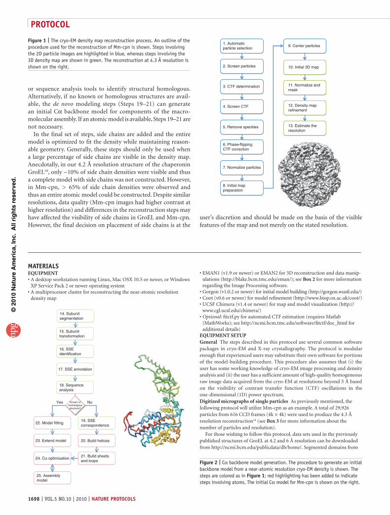
9. Center particles Figure 1 | The cryo-EM density map reconstruction process. An outline of the procedure used for the reconstruction of Mm-cpn is shown. Steps involving the 2D particle images are highlighted in blue, whereas steps involving the 3D density map are shown in green. The reconstruction at 4.3 Å resolution is shown on the right.

Figure 2 | Cα backbone model generation. The procedure to generate an initial backbone model from a near-atomic resolution cryo-EM density is shown. The steps are colored as in Figure 1; red highlighting has been added to indicate steps involving atoms. The initial Cα model for Mm-cpn is shown on the right.

MaterIalsEQUIPMENT

A desktop workstation running Linux, Mac OSX 10.5 or newer, or Windows XP Service Pack 2 or newer operating systemA multiprocessor cluster for reconstructing the near-atomic resolution density map

•

•

user’s discretion and should be made on the basis of the visible features of the map and not merely on the stated resolution.

Yes

15. Subunittransformation

16. SSEidentification

17. SSE annotation

22. Model fitting

23. Extend model

24. Cα optimization

25. Assemblymodel

19. SSEcorrespondence

20. Build helices

No

18. Sequenceanalysis

21. Build sheetsand loops

Known orhomologousstructure?

14. Subunitsegmentation

©20

10 N

atu

re A

mer

ica,

Inc.

All

rig

hts

res

erve

d.

protocol

nature protocols | VOL.5 NO.10 | 2010 | 1699

the 4.2 Å resolution structure of GroEL are also publically available for use in model generation and optimization at http://gorgon.wustl.edu.Determining the 1D structure factor In this protocol, it is important to determine the CTF parameters as accurately as possible. To do this, it is nec-essary to determine or calculate the 1D structure factor for the sample. This generally can come from one of three sources: an X-ray solution scattering experiment performed on the specimen, simultaneous fitting of several CCD frames at different defocuses or use of a structure factor from a different specimen. As this structure factor is normally only used to achieve better fit-ting of the CTF parameters, the final structure is not particularly sensitive to an imprecise structure factor.

For Mm-cpn, we manually fit the CTF for several CCD frames simultane-ously such that the derived structure factor at low resolution (~ 20 Å and beyond) agreed as well as possible (Fig. 4). This low-resolution structure factor was then averaged and combined with a standard curve at high resolution (in this case, an X-ray solution scattering curve from GroEL was used19). This process is documented in detail in the EMAN FAQ (http://blake.bcm.tmc.edu/emanwiki/EMAN1/FAQ). Again, as the structure factor is used only for CTF parameter fitting, and is not directly imposed on the model, there is little risk associated with use of a moderately inaccurate structure factor. EMAN2 incorporates a fully automated procedure for determining this estimated structure factor directly from the data.

proceDurereconstruction1| Select particles. To perform automated particle picking, a set of reference ‘template’ particles are required. These can be produced from a preliminary 3D model using makeboxref.py. The number of required references will vary depending on how different the particle appears when rotated, and based on user preference (more references → more accurate picking but longer runtimes). A set of manually selected reference particles from boxer was used in Mm-cpn. The following EMAN1 command performs reference-based particle selection. batchboxer input = 001.mrc refimg = ref.hed auto = 0.45,0.85,0.08 out-put = 001.hed dbout = 001.box, where 001.mrc is the input CCD frame; ref.hed is a set of reference particle images; 001.hed is the output containing the boxed-out particles from 001.mrc; 001.box is a text file containing the coordinates of the selected particles. Here, we specify 0.45, 0.85 and 0.08 as thresholds for automatic particle detection. These parameters vary from project to project, and are generally determined by trial and error using one or two CCD images or micrographs as representa-tives of the set.

The box size used in this process is based on the box size of the reference particles. Good box sizes to use are multiples of 2, 3, 5, 7 and 11, and should be divisible by 4. Odd box sizes are not supported in EMAN 1.x. The box should be ~50% larger than the particle. Note that EMAN2 requires box sizes ~2× larger than the particle for more accurate CTF correction, and this should be considered if EMAN2 may be used at a later time point. crItIcal step In EMAN, the IMAGIC20 file format is used by default for stacks of 2D images. Each of these files consists of a pair of .hed/.img files. When running an EMAN command, you may specify either the .hed or .img file, but do not run the same job on both, or you will process the same file twice. Similarly, if these files are renamed or moved, both files must be moved together. crItIcal step Detailed help for individual EMAN1 commands can be displayed by typing the command followed by ‘help’ in the console window.

2| Screen particles. Automatic picking does a reasonable job at selecting particles in most cases, but removing false positives, such as ice contamination, is necessary. Each CCD frame and the corresponding box database can be read into

Box 1 | EMAN1 VS. EMAN2 EMAN2 is the successor to EMAN1, and although it still follows most of the same principles as EMAN1, the specific details of how it should be used are substantially different from EMAN1. It incorporates a completely new CTF model, has an integrated workflow for image processing and a new modular infrastructure, giving users much more flexibility as they process their data. Note that EMAN2 is still in its very early release. All of our published near-atomic resolution structures were completed with EMAN1 (refs. 8–10,14,16). Moving forward, it is worth considering using EMAN2, although EMAN1 remains the more proven platform at this point in time. Regardless of platform, the material in this protocol will still provide useful information about the issues involved during processing, even if the specific commands have changed.

29. Model completion

model 28. Cα to atomic

30. Side chain registration

31. Model optimization

27. Rescale density map

32. Fix outliers

33. Fit model to density map

into a density map 26. Turn Cα model

Figure 3 | Atomic model generation. The procedure for generating an atomic model from a Cα backbone is shown. Steps are color coded as described in Figures 1 and 2. The final subunit model for Mm-cpn is shown on the right.

©20

10 N

atu

re A

mer

ica,

Inc.

All

rig

hts

res

erve

d.

protocol

1700 | VOL.5 NO.10 | 2010 | nature protocols

EMAN1’s boxer and screened manually. False positives are deselected (shift-left-click on the particle in boxer) and the final particle sets are then saved.

3| Determine the CTF parameters. Images acquired on transmission electron microscopes are density projections convoluted with the microscope’s CTF. To produce a corrected reconstruction, the CTF parameters must be first estimated. The follow-ing command estimates the CTF parameters automatically21 (requires Matlab from The MathWorks) (the fitctf program (no .py extension) provided with EMAN1, is an alternative, but results are less accurate and require more adjustment by hand):fitctf.py --sf = ./wt-alfx-new.sf --apix = 1.33 --cs = 4.1 --voltage = 300 --max_s = 0.125 --show_fit *.img, where wt-alfx-new.sf is a text file containing a 1D structure factor for the specimen; 1.33 is the Å per pixel value; 4.1 is the objective lens spherical aberration coefficient value of the microscope in mm; 300 is the accelerating voltage of the microscopy in keV; 0.125 is the highest frequency (in the unit of 1/Å) of the CTF curve to be used in the fitting, and must be determined by trial and error; and *.img are all the particle images in the .img format. The estimated CTF parameters were stored in a file called ‘ctfparm.txt’ in the same directory as the particles.

4| Screen the CTF. Similar to the particle selection process, CTF parameter estimation produces inaccurate parameters in some cases. The automatically determined parameters must be manually screened using the EMAN1 program ctfit. The eight CTF parameters can be manually adjusted in ctfit to best match the particle power spectrum. Although it is clearly desirable to have CTF parameters as accurate as possible, the level of accuracy provided by visual inspection is sufficient to insure proper phase flipping. The envelope function widths (known as experimental B-factors22) from different images will normally be quite similar for images collected on the same microscope of the same specimen. There may be a moderate correlation with defocus. As there may be some apparent interdependence between Fourier amplitude and experimental B-factor, in general, strive to keep the experimental B-factors in the same general range unless the data clearly requires a significant variation.

5| Remove speckles. Cosmic ray–derived X-rays can produce very bright pixels in CCD frames. These are removed before reconstruction on the boxed-out particle stacks using the following EMAN1 command:speckle_filter.py 001.hed 001.fix.hed; where 001.hed is the input particle images and 001.fix.hed is the output images.

6| Correct CTF with phase flipping. CTF correction is a two-step process. This first step performs the phase flipping portion of CTF correction and stores the CTF parameters in the headers of the individual particles for later use in CTF Fourier ampli-tude correction. The following EMAN1 command performs the first half of CTF correction.applyctf 001.fix.hed 001.fix.hed inplace flipphase setparm invertThe ‘invert’ option should be used if the protein density appears dark with a light background when viewing the individual parti-cle images. In the EMAN convention, protein density should be white. The ‘inplace’ argument is used when the same file is speci-fied as input and output so as to overwrite the input images.

7| Normalize particles. Particle densities are rescaled so that the mean value around the edge of each particle is 0 and the standard deviation is 1.0. This can be done using the EMAN1 program proc2d. Having the mean solvent density at zero is important for later image processing steps, which occasionally perform zero-padding of the particle images. proc2d 001.fix.hed 001.fix.hed inplace edgenorm.

Box 2 | IMAGE PRoCESSING SoFTWARE EMAN1 is one of several different packages that have been developed for single-particle reconstruction. Imagic20, Spider36 and Frealign37 are the other commonly used packages for this purpose, but several others have been developed as well. Each package has its own specific strengths and weaknesses. EMAN1, and even more so EMAN2, offer well-defined processing pipelines for the single-particle reconstruction task; these are fairly straightforward for beginners to learn, and produce accurate results. EMAN1 has been used for a majority of the published structures at better than 5 Å to date8–10,14–17; Frealign, optimized for icosahedral particles, has been used for processing several viruses12,15.

102

101

Inte

nsity

1/Inf 1/20.00 1/10.00

S (1/Å)

1/6.67 1/5.00

Figure 4 | CTF curve. The experimental CTF curve, shown in gray, is plotted against the fit CTF curve (black) for particles from a typical CCD frame.

©20

10 N

atu

re A

mer

ica,

Inc.

All

rig

hts

res

erve

d.

protocol

nature protocols | VOL.5 NO.10 | 2010 | 1701

8| Prepare to generate a starting map. For convenience, create a subdirectory called ‘raw’ and move all the preprocessed particles images (*.fix.hed/img) into ‘raw’ directory. A ‘start.hed’ file containing all the particle images from the entire set of micrographs and/or CCD frames can be created. This file should be an LST format text file.

9| Roughly, center a portion of particle images for better initial model generation in EMAN1 using the following command:cenalignint start.hed frac = 0/50 mask = 96; where 0/50 means it will take the first 1/50 of the images to generate the initial model; ‘mask = 96’ is the radius of the mask, which is equivalent to half the box size in pixels. The ‘frac’ may be adjusted to produce the desired number of particles for initial model generation. In most cases only a subset will be required, but aside from additional time requirements, there is no harm in using the entire set. The centered particles are saved in a file called ali.hed, and are used only for initial model generation.

10| Determine the initial 3D map. The technique mentioned here will work only on particles with C3 or greater symmetry. For particles with Dn symmetries (Cn symmetry with an additional ‘n’ twofold symmetries), only the corresponding C-symmetry will be imposed in this step. The EMAN1 programs starticos and startoct are provided for particles with icosahedral or octahedral symmetry, respectively.

An initial 3D density map for Mm-cpn with D8 symmetry was constructed from the roughly aligned images using the following command: startcsym ali.hed 50 sym = d8, where sym is the symmetry for the initial model.

The number ‘50’ refers to the number of particles to search for in the top and side views; generally, this will be < 10% of the particles in ali.hed. UCSF Chimera23 was used to examine the initial Mm-cpn model (threed.0a.mrc).

For particles with less than C3 symmetry, or for sufficiently symmetrical structures in which initial model generation works poorly, refer to Box 4 for further information.

11| Normalize and mask the density map. In preparation for 3D refinement, the initial map density values are normalized and masked to reduce noise using the following EMAN1 commands. The first command normalizes the density based on molecular weight, whereas the second command applies a mask around the particle to remove noise.volume threed.0a.mrc 1.33 set = 960; where 1.33 is the Å per pixel value and ‘set = 960’ refers to the molecular weight of the protein in kDa. proc3d threed.0a.mrc threed.0b.mrc apix = 1.33 automask2 = < rad > , < thr > , < shls > < rad > , < thr > , < shls > must be determined iteratively via trial and error. < rad > is the radius in pixels of a sphere sufficient-ly large to come in contact with some portion of the model, but not extending outside the model. < thr > is an isosurface

Box 3 | NUMBER oF PARTICLES AND RESoLUTIoN The reported number of particles to achieve a given resolution varies, because it depends on several factors including the particle conformational homogeneity, the symmetry of the particle, the postreconstruction averaging due to the presence of symmetry inher-ent in the asymmetric unit of the particle, the types of electron microscope and recording medium, the software used to carry out the reconstruction, and the experience of the users. The size of the particles has a fairly small influence on the required number of particle images for a given resolution because they are linearly related. For a subnanometer-resolution reconstruction of an icosahedral particle, it takes only a few hundred high-quality particles38.

The Mm-cpn reconstruction associated with this protocol used ~30,000 particles, but had D8 symmetry, meaning ~480,000 monomeric subunits (asymmetric units) were averaged to generate the map14. Compared with other chaperonin maps at this resolution range, the total number of asymmetric units for the final map is similar8,10,14, although it is a factor of 3–30× smaller than those used to generate the icosahedral virus particle maps6,7,9,13,15,16. The large difference among these studies is attributable to a combination of reasons, as stated.

Box 4 | INITIAL MoDEL GENERATIoN For particles with less than C3 symmetry, or for sufficiently symmetrical structures in which initial model generation works poorly, a range of other methods can be applied; a detailed discussion is too lengthy for this protocol. Briefly, the preferred approach in EMAN1 is to use makeinitialmodel.py to generate a randomized starting model, refine from that, and then repeat the process several times to attempt to achieve a consensus. This method has been fully automated in EMAN2, and is very reliable in the majority of cases, regardless of symmetry. Another approach is to use single-particle tomography to determine a low-resolution structure39. Random conical tilt is another popular method for this task40, but is not directly supported in EMAN1. Finally the ‘angular reconstitution’ method is another approach41, which is implemented as startAny in EMAN1. However, we no longer suggest using this technique, as when it does produce an incorrect model, it has a high probability of being near a local minimum and getting ‘stuck’ in an incorrect structure upon 3D refinement.

©20

10 N

atu

re A

mer

ica,

Inc.

All

rig

hts

res

erve

d.

protocol

1702 | VOL.5 NO.10 | 2010 | nature protocols

threshold ≤ the threshold used to visualize the model. < shls > is the number of 1-voxel shells to extend the model beyond the core shown by the isosurface. Note that this will include only portions of the structure connected to the original sphere by density above the specified threshold. crItIcal step Detailed instructions on how to choose the best parameters for automatic masking are described in the EMAN1 FAQ.

12| Refine the map. In an iterative approach, the center and orientations of individual particle images are refined against the previous iteration’s 3D density map. Shown below is the sequence of EMAN1 refinement commands used for Mm-cpn. Initial refinement rounds have parameters for rough refinement of the particle shape and are quite fast. The first four rounds of refinement are used to determine the correct low-resolution shape, and have parameters designed to eliminate initial model bias. Each subsequent command makes the orientation search finer and finer, and eliminates a larger portion of the input particles, targeting higher resolution. The precise sequence below is not necessarily optimal; it is simply what was used for the published Mm-cpn structure. The final rounds require considerable computation.

refine 4 mask = 96 proc = 128 hard = 25 sym = d8 refmaskali ang = 4.5 pad = 256 classkeep = 1 classiter = 8 xfiles = 1.33,960,99 amask = 40,0.8,20 shrink = 4 phaseclsrefine 8 mask = 96 proc = 128 hard = 25 sym = d8 refmaskali ang = 3 pad = 256 classkeep = 1 classiter = 5 xfiles = 1.33,960,99 amask = 40,0.8,20 shrink = 2 phaseclsrefine 12 mask = 96 proc = 128 hard = 25 sym = d8 refmaskali ang = 3 pad = 256 classkeep = 1 classiter = 5 xfiles = 1.33,960,99 amask = 40,0.8,20 phaseclsrefine 20 mask = 96 proc = 128 hard = 12 sym = d8 refmaskali ang = 1.40625 pad = 256 classkeep = 0.8 classiter = 3 xfiles = 1.33,960,99 amask = 40,0.8,20 dfilt ctfcw = ./wt-alfx-new.sf refine

The first number after the refine command (4, 8, 12 and 20) refers to the number of iterations for the refinement. For example, in the second command ‘refine 8 …’ picks up where ‘refine 4’, the previous command, left off and runs four more iterations; ‘mask’ specifies the radius of the circular mask in pixels to apply; ‘proc’ is the number of processors available/configured as per the EMAN1 documentation; ‘hard’ is a mean phase error for excluding class-averages from the 3D recon-struction (25 is a typical value for most projects); ‘sym’ is the symmetry of the particle; ‘refmaskali’ will use the mask from the previous iteration during alignment for better accuracy; ‘ang’ is the angular separation of the projections used for clas-sification (smaller values are used as resolution improves); ‘pad’ specifies the box size to be used for the 3D reconstruction (typically, ~25% larger than the particle box size); ‘classiter’ eliminates initial model bias (3 is generally the minimum value though larger values will strongly reduce bias at the cost of resolution); ‘xfiles’ specifies volume normalization parameters: Å per pix, mass in kDa and an optional alignment parameter generally disabled by specifying 99; ‘amask’ specifies the same 3 parameters used for automasking in Step 11; ‘phasecls’ and ‘dfilt’ are options to select different image similarity metrics for classification (dfilt is generally the best, but is also the slowest); ‘ctfcw’ specifies the same 1D structure factor file used when determining CTF parameters for Fourier amplitude correction; and ‘refine’ will do subpixel alignment of the particle translations for classification (this may have a significant impact for high-resolution reconstructions, but at a substantial computational cost).

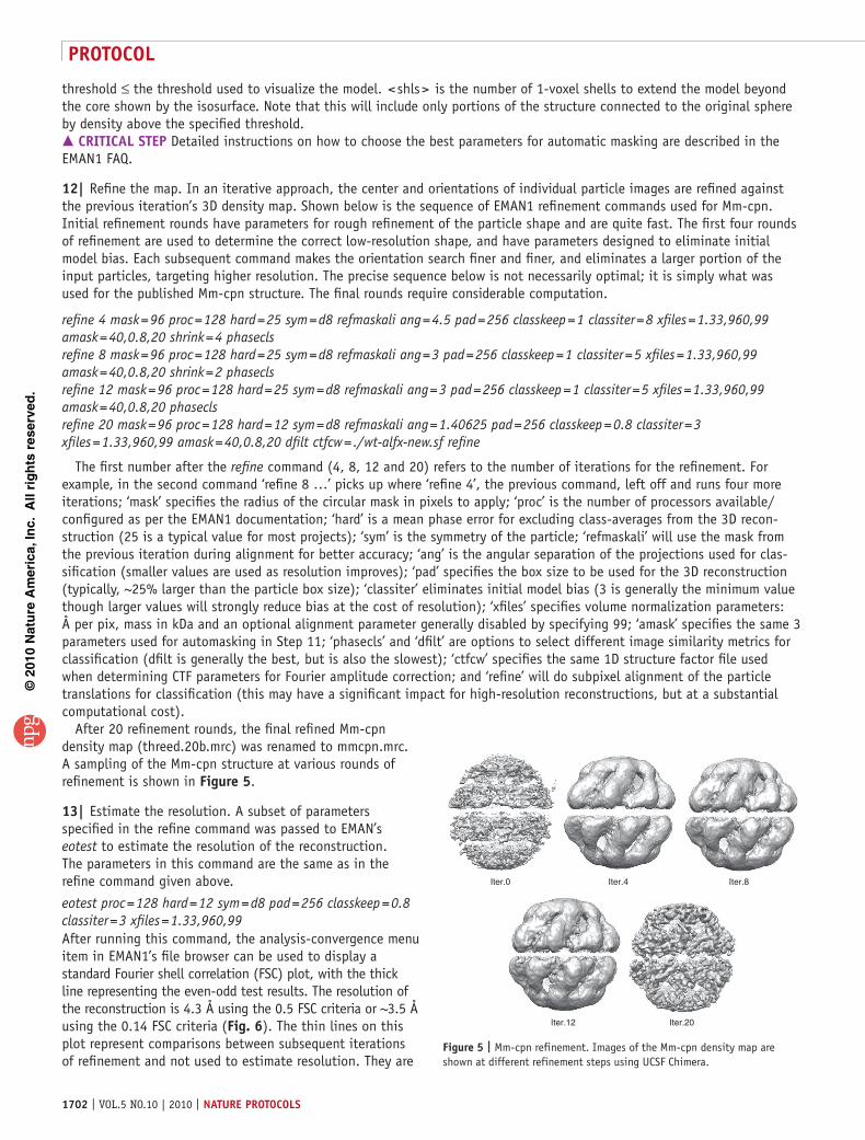
After 20 refinement rounds, the final refined Mm-cpn density map (threed.20b.mrc) was renamed to mmcpn.mrc. A sampling of the Mm-cpn structure at various rounds of refinement is shown in Figure 5.

13| Estimate the resolution. A subset of parameters specified in the refine command was passed to EMAN’s eotest to estimate the resolution of the reconstruction. The parameters in this command are the same as in the refine command given above.

eotest proc = 128 hard = 12 sym = d8 pad = 256 classkeep = 0.8 classiter = 3 xfiles = 1.33,960,99After running this command, the analysis-convergence menu item in EMAN1’s file browser can be used to display a standard Fourier shell correlation (FSC) plot, with the thick line representing the even-odd test results. The resolution of the reconstruction is 4.3 Å using the 0.5 FSC criteria or ~3.5 Å using the 0.14 FSC criteria (Fig. 6). The thin lines on this plot represent comparisons between subsequent iterations of refinement and not used to estimate resolution. They are

Iter.0 Iter.4

Iter.12 Iter.20

Iter.8

Figure 5 | Mm-cpn refinement. Images of the Mm-cpn density map are shown at different refinement steps using UCSF Chimera.

©20

10 N

atu

re A

mer

ica,

Inc.

All

rig

hts

res

erve

d.

protocol

nature protocols | VOL.5 NO.10 | 2010 | 1703

used instead to judge whether the refinement has converged or whether more iterations are required.

Building a ca model14| Segment a subunit. The first step in building a model in a cryo-EM density map is to identify a single protein subunit. Boundaries between subunits can be readily identi-fied as a drop off in density can be seen at the edge of a subunit. Using the ‘Volume Eraser’ tool in UCSF Chimera, approximately one subunit was isolated from the Mm-cpn reconstruction (‘mmcpn.mrc’) by erasing density not belong-ing to the subunit. The segmented subunit was saved as ‘mmcpn-monomer.mrc’ under the option ‘Save Map’ in the ‘Volume Viewer’ of Chimera.

At this stage, it is possible to segment all subunits, although for the subsequent model-building steps, it is advisable to build one model at a time. These initial segmentations are meant to be approximate as the final models may alter the original subunit interpretations. crItIcal step Do not try to be too exact. Crude subunit segmentation is adequate and avoids removing too much density. It is better to segment slightly more than one subunit than slightly less than one subunit.

15| Transform the segmented subunit map into an even cubic density map and reset the origin using proc3d in EMAN1.proc3d mmcpn-monomer.mrc mmcpn-monomer128.mrc clip = 128,128,128 origin = 0,0,0; where the file names are the input and output files, respectively, and ‘clip’ specifies the box size, an even number ~10% greater than the largest dimension of the segmented subunit. The option ‘norm’ may also be included after the clip option to normalize the data. To maximize compat-ibility with other modeling programs, the origin of the segmented subunit is reset with ‘origin = 0,0,0’.

16| Identify SSEs with SSEHunter3. Using the ssehunter3.py utility in EMAN1, a visual representation of SSEs in a density map can be calculated. Map sizes between 483 and 1603 generally require < 15 min to run on a modern desktop. The follow-ing command was used to generate a set of pseudoatoms, SSEHunter’s default output, for a single Mm-cpn subunit.ssehunter3.py mmcpn-monomer128.mrc 1.33 4.3 1.0; where 1.33 is the Å per pixel sampling of the map, 4.3 is the resolution of the map (in Å) using the 0.5 FSC criterion and 1.0 is the highest isosurface value at which all density of the segmented subunit appears to be connected (obtained visually from Chimera, ~3.5 σ above the mean density for Mm-cpn). SSEHunter will return a set of pseudoatoms (in PDB format) with scores assigned between − 3 and 3 (encoded in the B-factor column of the PDB file). These values represent the likelihood of a density region to be either an α-helix (0–3) or a β-sheet ( − 3 to 0).

Optionally, a graphical version of SSEHunter has been incorporated into Gorgon (http://gorgon.wustl.edu/) and UCSF’s Chimera (Fig. 7a). crItIcal step There should be fewer pseudoatoms (~50%) than amino acids in the SSEHunter output file. The threshold parameter may need to be tweaked if the number of pseudoatoms is too high.

17| Annotate the SSEs. Pseudoatoms with similar SSEHunter values are grouped into SSE using SSEBuilder3. SSEBuilder is available as a plug-in to UCSF Chimera (distributed with EMAN; detailed instructions on installing the SSEBuilder plug-in can be found at http://ncmi.bcm.edu/software/AIRS) or as part of Gorgon. In Gorgon, pseu-doatoms are automatically colored from blue ( − 3, β-sheet) to white (0) to red

1.0

0.9

0.8

0.7

0.6

0.5

Fou

rier

shel

l cor

rela

tion

0.4

0.3

0.2

0.1

00 0.05 0.10 0.15 0.250.20

1/Resolution (1/Å)

0.30

3.5

4.3

Figure 6 | FSC curve. The FSC curve from the final refined density map of Mm-cpn is shown. Using the 0.5 (solid line) and 0.14 (dashed line) criteria, the map has a resolution of 4.3 and 3.5 Å, respectively.

a b

Figure 7 | SSE identification. For Mm-cpn, SSEHunter (an EMAN program) was run as a plug-in to UCSF’s Chimera. The results are shown in a wherein the red spheres represent helix-like regions and the blue spheres represent sheet-like regions. SSEBuilder, also an EMAN program, run as plug-in in UCSF’s Chimera, is shown in b. Regions of similar scoring pseudoatoms from SSEHunter are grouped and then built using SSEBuilder. Helices are shown as green cylinders. Six pseudoatoms are highlighted in green and are shown in the SSEBuilder dialog before constructing a helix.

©20

10 N

atu

re A

mer

ica,

Inc.

All

rig

hts

res

erve

d.

protocol

1704 | VOL.5 NO.10 | 2010 | nature protocols

(3, α-helix). The intensity of the color reflects the score and the confidence of the prediction. Multiple atoms with similar SSEHunter scores that appear to belong to the same SSE are grouped, assigned an ID, labeled as an α-helix or a β-sheet and then constructed (Fig. 7b). SSEs are shown as Virtual Reality Modeling Language (VMRL) objects (cylinders and planes for helices and sheets, respectively).

To achieve the Gorgon pseudoatom color-coding scheme in Chimera, use the ‘Render by Attribute’ option to display the ‘B-factor’ attribute such that blue is the most negative value (sheet) and red is the most positive value (helix).

In Mm-cpn, 17 α-helices and 5 β-sheets were identified and built with the SSEBuilder plug-in for Chimera. crItIcal step When building SSEs, the minimum number of pseudoatoms is three for an α-helix and five for a β-sheet. False-positive results may occur, so only select pseudoatoms that look like SSEs in the density map; α-helices are long rods and β-sheets are thin, curved surfaces.

18| Analyze the primary sequence. The sequence of the pro-tein of interest can be submitted to various sequence search engines such as PsiBlast24 to determine whether a known or related structure exists. Several metatools exist that will perform the search and subsequent homology modeling if a structural homolog is found. In the event that a known structure exists or a structural homolog is identified and modeled, skip to Step 22.

However, if no known or homologous structure is available, predicting SSEs from the sequence is necessary and Steps 19–21 must be completed; Step 22 is omitted. Any number of web-based programs can be used to predict secondary structure in-cluding SSPro25, JPred26, PHD27, PsiPred28 or Predator29. Alternatively, Gorgon contains a tool that will remotely run the sequence prediction. In all cases, the results may be formatted as either a PDB file or a ‘seq’ file that contains both the amino acid and secondary structure prediction.

For Mm-cpn, a homology model was previously constructed30 using the thermosome KS-1 structure31 (PDB ID: 1Q3Q) as a template with the fully automated protein homology-modeling server, SWISS-MODEL (http://swissmodel.expasy.org/)32. Steps 19–21 were omitted; model building for Mm-cpn continued with Step 22. crItIcal step A consensus alignment built from multiple predictions may be better than the results from a single secondary structure prediction server.

19| Generate a SSE correspondence (required if no known or homologous structure is available). After identifying SSEs in both the density map and the sequence of the subunit in question, the next step is to identify the optimal sequence to structure correspondence33. This step provides the initial anchor points used to place Cα atoms and construct a protein backbone trace in Steps 20 and 21.

The ‘Identify SSE Correspondence’ tool in Gorgon will read in the SSEBuilder results and the sequence/prediction file to calculate the best matching SSEs (Fig. 8). The user will be prompted to enter four files: the 3D sheet locations (*.sse), 3D helix locations (*.wrl), the cryo-EM skeleton (*-skeleton.mrc) from SSEHunter and the sequence/prediction from the previous step. Once these files have been entered, Gorgon will display possible correspondences. The results are listed in order of best correspondence to worst. The user can select individual α-helices in the main viewer window of Gorgon or in the results to highlight the individual correspondence. To assess the correspondence, one can examine the lengths of the SSEHunter helices compared with the sequence-predicted helices. Ideally, correctly paired helices will be within 1–2 amino acids in size.

In a correspondence, one or more helices may have an incorrect correspondence. At this point, the user may ‘lock-in’ the correct sequence-structure correspondence by checking the ‘constrain’ box in the SSE correspondence results window. The correspondence search can then be rerun, producing results with only the constrained sequence-structure mapping. This process is relatively quick ( < 5 s for most cases) and can be done repeatedly until the user is satisfied with the correspondence. crItIcal step An SSE correspondence cannot be saved, although a Gorgon session containing all of the data and correspondence can be saved and reloaded.

Figure 8 | SSE correspondence. The result from an SSE correspondence search from Gorgon is shown. The correspondence search shown here was performed on the apical domain of the 4.2 Å resolution structure of GroEL. Helices are shown as cylinders and potential connectivity is shown as colored lines. A corresponding color scheme for these elements is shown in the SSE correspondence window on the right.

©20

10 N

atu

re A

mer

ica,

Inc.

All

rig

hts

res

erve

d.

protocol

nature protocols | VOL.5 NO.10 | 2010 | 1705

20| Place Cα atoms in helices (required if no known or homologous structure is available). Placing Cα atoms in the den-sity map is divided into three phases: helix assignment (Step 20), strand/loop assignment (Step 21) and Cα optimization (Step 22). Gorgon offers several ways to place and manipulate individual Cα atoms in the density map with its ‘Semi-automated atom placement’ tool. This tool is divided into two primary sections: a sequence viewer and an atom panel (Fig. 9). A global view of the predicted secondary structure is represented in the topmost portion of the sequence viewer. Helices are colored from the N- (blue) to C- (red) termini. The gray box in the global sequence view indicates the region shown in the local sequence view just below the global sequence view. In the local sequence view, clicking on one of the α-helices will highlight the corresponding sequence; clicking on the helix in the main Gorgon viewer will also select the corresponding sequence.

Using the ‘Helix Editor’ tab in the ‘Semi-automated atom placement’ tool, assign a selected sequence to the position of the cylinder (helix) in the density map (Fig. 9a). If necessary, adjust the helix length before assigning the helix atoms by chang-ing the starting and stopping residues of the helix. It may also be necessary to flip the direction of the helix with the ‘Flip’ option in the atom panel.

Individual helix positions can be adjusted by selecting the residues within a helix and moving them with the ‘Rotate and Translate’ operations in the ‘Position’ tab. Complete assigning for all α-helices before assigning any other atoms. Note that the sequence in the local sequence viewer turns black to indicate that atoms have been placed in the density map.

21| Place Cα atoms in sheets and loops (required if no known or homologous structure is available). For the purposes of modeling a Cα backbone, β-strands are treated the same as loops. Extending from the assigned residues in the α-helices, assignment of the remaining residues is accomplished with the ‘Atomic Editor’ and ‘Loop Editor’. With the ‘Atomic Editor’, the last assigned residue before an unassigned section of sequence is selected (Fig. 9b). The next unassigned residue is shown in green in the panel and a list of possible positions along the density skeleton, for which a Cα-Cα distance is satisfied, is shown as a set of white and blue spheres. The current choice is shown in blue; the user can toggle through the choices in the ‘Atomic Editor’ tab until the desired position is found. The process is repeated until all residues in a loop are assigned. Alternatively, loops may be assigned using the ‘Loop Editor’. The endpoints of the loops can be selected from which the user can then draw out an approximate path through the density (Fig. 9c). crItIcal step Atoms are placed along a skeleton that runs through the medial axis of the density. Although the true Cα-Cα distance is 3.8 Å, it may be necessary to adjust the Cα distance in Gorgon for ~3.5 Å initial placement and then later readjust it to ~3.8 Å.

22| Fit an atomic model (required if a known or homologous structure is available). Fitting of a known or related structural model can be accomplished using a wide range of computational tools. The Mm-cpn homology model, a PDB file constructed in Step 18, was fit to the segmented density subunit with EMAN1’s Foldhunter2 using the following command:foldhunter.py mmcpn-monomer128.mrc mmcpn-homology-model.pdb res = 4.3 apix = 1.33, where the homology model is fit to the density, apix is the Å per pixel value and res is the resolution of the map. A transformed PDB file, denoted by default with the prefix ‘fh-’ is outputted.

Verification of the fit is achieved by visually examining the correspondence of SSEs in the model and map. Differences and missing residues in the model are addressed in later steps.

a b c

Figure 9 | Modeling in Gorgon. (a–c) Gorgon contains several methods for assigning atoms to the density. In a, the ‘Helix Editor’ is shown. In b, the ‘Atomic Editor’ is shown, whereas c shows the ‘Loop Editor’ from Gorgon.

©20

10 N

atu

re A

mer

ica,

Inc.

All

rig

hts

res

erve

d.

protocol

1706 | VOL.5 NO.10 | 2010 | nature protocols

23| Extend the Cα trace. With atomic models, portions of the model may be missing, particularly at the termini. In these cases, Steps 20 and 21 may be used to build any missing residues before proceeding, as was done for the terminal residues of Mm-cpn. If no residues are missing, only optimization of Cα placement is necessary.

24| Optimize Cα positions. After all Cα atoms have been assigned, atom positions are adjusted such that they fit the density optimally while maintaining reasonable Cα-Cα bond distances (~3.8 Å) and angles (~60–120° between three consecutive Cα), proper secondary structure features and no atom/bond clashes. This process can be done in any molecular modeling toolkit such as Gorgon or Coot34.

Optimization of Cα positions begins with SSEs and extends to loops. In particular, the pitch of the model helices needs to register well with the pitch of the helix observed in the density. In the event β-strands are resolved, the distance between neighboring strand Cα atoms should be between 4.5 and 5 Å. In models utilizing a known or homologous model, such as Mm-cpn, entire SSEs are first moved to register with those identified by SSEHunter. Once the model’s SSEs have been fit to the density map, the remaining Cα can then be moved individually to best fit the density. To aid in this procedure, the density skeleton calculated in SSEHunter and used in the SSE correspondence step can provide a clear path.

In Gorgon, groups of atoms are dragged into position with the mouse. Alternatively, groups of atoms may be moved using the ‘Position editor’ in Gorgon’s ‘Semi-automated atom placement’ tool. In Coot, the same process can be done using the ‘Rotate/Translate Zone’ feature by selecting the starting and ending points of a set of consecutive residues and transforming them as a single unit using a set of six sliders that control translation and rotation. crItIcal step In Gorgon, Cα-Cα distance is indicated by color. Red bond distances are too long, blue bonds are too short and white bonds are approximately the right length.

25| Build an assembly model. Once the initial Cα subunit model has been built, it can be fit back into the context of the full cryo-EM density map. In total, 16 copies of the initial Cα model of a Mm-cpn subunit were loaded into UCSF’s Chimera, manually moved into the approximate location of a subunit and fit to the density using the ‘Fit in map’ option.With Mm-cpn, Steps 24 and 25 were iterated over eight complete cycles of Cα backbone model optimization until no inter- and intra-subunit clashes were evident. The final refined backbone model was then saved as a PDB file.

Building an atomic model26| Create a synthetic density map. Using the complete, refined Cα backbone model, the density map needs to be rescaled in Fourier space to enhance the high-resolution information, such as side chains, for atomic model building and optimization. Using EMAN1, the Mm-cpn Cα model is first blurred to approximately the same resolution as the density map using the following command: pdb2mrc mmcpn.pdb mmcpn-simulated.mrc res = 4.3 apix = 1.33 box = 192, where the resolution of the density map is 4.3 Å for Mm-cpn, 1.33 is the Å per pixel sampling of the density map and the size of the density map for Mm-cpn is 192 (ref. 3).

27| Rescale the density map values. Once the synthetic density map has been generated, 1D structure factors are generated and applied to the original density map. To do this in EMAN1, use the following commands:

proc3d mmcpn-simulated.mrc junk.mrc calcsf = mmcpn-sf.txt apix = 1.33proc3d mmcpn.mrc mmcpn-rescaled.mrc setsf = mmcpn-sf.txt apix = 1.33proc3d mmcpn-rescaled.mrc mmcpn-lp.mrc lp = 4.3 apix = 1.33proc3d mmcpn-lp.mrc mmcpn-final-map.mrc mult = 0.3,

where 1.33 is the Å-per-pixel sampling of the density map, lp = 4.3 is a low-pass filter at 4.3 Å (the resolution of the density map) and 0.3 is a constant that is approximately the inverse of the maximum density value in the map value.

The first command generates a text file containing the 1D structure factors of the synthetic map, whereas the second command applies it to the original density map. The next step applies a low-pass filter at the defined resolution, 4.3 Å in the case of Mm-cpn. In the final step, the density values of the map are rescaled so that the positive density values range between 0 and 1. crItIcal step Near-atomic resolution is not required for map rescaling. This type of rescaling can be done as long as structure factors can be calculated from a structural model.

28| Convert the Cα model to an atomic model. Using SABBAC35, a web-based Cα to backbone builder (http://bioserv.rpbs.univ-paris-diderot.fr/cgi-bin/SABBAC), a full atomic model is reconstructed based on the optimized Cα model.

29| Complete the model. To repair missing or unassigned residues in the previous step, the model is loaded into Coot. Missing residues are added with the ‘Add residue’ option in Coot. All residues are added as alanines so that the ‘Simple mutate’ function in Coot can then be used to assign the appropriate residue ID. To complete the assignment, residues are moved using the ‘Rotate/Translate Zone’ option such that it forms a peptide bond with the neighboring residues.

©20

10 N

atu

re A

mer

ica,

Inc.

All

rig

hts

res

erve

d.

protocol

nature protocols | VOL.5 NO.10 | 2010 | 1707

For Mm-cpn, a complete atomic model for residues 1–532 was produced.

30| Register side chain positions. The resulting subunit atomic model is optimized to best fit the rescaled density map. In the ‘Refine/Regularize Control’ menu of Coot, torsion restraints, planar peptide restraints and Ramachandran restraints can be enforced. Main chain restraints are selected when refining atoms in the corresponding type of secondary struc-ture. Once the modeling parameters are set, stretches of residues are optimized using the ‘Real Space Refine Zone’ option (Fig. 10a). Similar to the Cα optimization step, optimization of the atomic model starts with the α-helices and proceeds to β-stands and then to loops. All main chain and side chain atoms are fit such that (1) no atoms are outside the density and (2) unoccupied density is minimized. This procedure is repeated until all atoms/amino acids fit well to the density. crItIcal step Try to select an entire SSE for refinement. Up to ~20 amino acids can be refined at one time in Coot.

31| Optimize an atomic model. Once the atoms are suitably placed, side chain positions can be optimized using the ‘Rotamers’ option in the ‘Model/Fit/Refine’ panel. Rotamers that most closely resemble the currently placed side chain are selected. In combination with this step, the main chain atoms may need to be improved as described in the previous section.

32| Fix outliers. The Ramachandran plot in Coot, found under the ‘Validate’ menu, will plot all amino acids and show out-liers, denoted by their red color. Clicking on these red points will automatically recenter the model on the selected residue in the main viewer window. As described in the previous section, refine outlier residues using the ‘Real Space Refine Zone’ option. Alternatively, ‘Regularize Zone’ can be used to improve short stretches of residues. In either case, refinement at this level should only be done over a small (3–5) number of amino acids. Several iterations of this and the previous step may be required to optimally place all atoms. For Mm-cpn, over 85% of the residues had favorable Phi-Psi angles and > 98% of all residues had acceptable Phi-Psi angles (Fig. 10b).

33| Fit all models back into the rescaled density map. As in Step 25, all atomic models (PDB files) are fit back into the den-sity map using either manual or automated procedures. For Mm-cpn, 16 copies of the final atomic model of a Mm-cpn subunit were loaded into UCSF’s Chimera and fit to the density using the ‘Fit in map’ option. The final was structure is then saved as a PDB file and deposited in the PDB.

● tIMInGEach data set is different and the exact parameters used in processing different data sets will vary. As such, the amount of time required for each step will vary considerably based on the sample, number of particles, resolution and the number of processors available. For Mm-cpn, the entire process took ~6 months once good freezing conditions were obtained for the sample. Selecting the 2D images and calculating the CTF required ~2 weeks, and processing the data required ~4 weeks using 200 CPUs on a large Linux cluster. Construction of the initial homology model, fitting to the density and initial Cα adjustments required ~4 weeks on a desktop workstation. Generation and optimization of the final atomic model required ~8 weeks.

antIcIpateD resultsFollowing this protocol, a user should be able to produce a near-atomic resolution cryo-EM density map and an atomistic model of the protein subunits with reasonable stereochemistry, similar to that of Mm-cpn. This procedure is not restricted to any particular sample type, although larger macromolecular assemblies will take longer to reconstruct and analyze owing to their size. Similar approaches and results have been applied to other chaperonins (GroEL10 and TRiC8), as well as viruses (bacteriophages ε15 (ref. 9) and bacteriophage P-SSP7 (ref. 16)). The protocol was designed to be modular; the analysis and modeling steps can

a bFigure 10 | Optimization with Coot. Coot was used to adjust main chain and side chain atom positions to optimize the fit of the atomic model in the density map of Mm-cpn. Shown in a is a screenshot using the ‘Real Space Refine Zone’ tool in Coot, whereas b shows the corresponding Ramachandran plot.

©20

10 N

atu

re A

mer

ica,

Inc.

All

rig

hts

res

erve

d.

protocol

1708 | VOL.5 NO.10 | 2010 | nature protocols

be applied to near-atomic resolution density maps from any imaging technique including X-ray crystallography. Similarly, the density map reconstruction step may also be applied to cryo-EM specimens not targeting near-atomic resolutions.

In reference to the final atomic model, several features are of note. Although individual atoms are not resolved at this resolution, the overall backbone trace should be relatively unambiguous. However, side chain density is likely to be more ambiguous. In Mm-cpn, positively charged residues were well resolved, whereas glycines and prolines were almost associated with ‘breaks’ or discontinuities in the density map. The rate for observing the remaining side chains in the density map was ~75% as compared with nearly 100% for positively charged amino acids.

Consulting the various user guides and documents for the individual software packages will help users select the optimal parameters for their project.

acknoWleDGMents This research was supported by grants from the National Institutes of Health through the Nanomedicine Development Center (PN1EY016525), the Nanobiology Training Program (R90DK71504), the Institute of General Medical Sciences (R01GM079429, R01GM080139), the National Center for Research Resources (P41RR002250) and the National Science Foundation (IIS-0705644, IIS-0705474).

autHor contrIButIons M.L.B. developed Gorgon, the cryo-EM–based modeling protocol and modeled Mm-cpn. S.J.L. developed EMAN and the reconstruction protocol. J.Z. performed the image processing and reconstructions for Mm-cpn. All authors contributed to the preparation of the paper.

coMpetInG FInancIal Interests The authors declare no competing financial interests.

Published online at http://www.natureprotocols.com/. Reprints and permissions information is available online at http://npg.nature.com/reprintsandpermissions/.

1. Chiu, W., Baker, M.L., Jiang, W., Dougherty, M. & Schmid, M.F. Electron cryomicroscopy of biological machines at subnanometer resolution. Structure 13, 363–372 (2005).

2. Jiang, W., Baker, M.L., Ludtke, S.J. & Chiu, W. Bridging the information gap: computational tools for intermediate resolution structure interpretation. J. Mol. Biol. 308, 1033–1044 (2001).

3. Baker, M.L., Ju, T. & Chiu, W. Identification of secondary structure elements in intermediate-resolution density maps. Structure 15, 7–19 (2007).

4. Baker, M.L. et al. Architecture of the herpes simplex virus major capsid protein derived from structural bioinformatics. J. Mol. Biol. 331, 447–456 (2003).

5. Ludtke, S.J., Serysheva, I.I., Hamilton, S.L. & Chiu, W. The pore structure of the closed RyR1 channel. Structure 13, 1203–1211 (2005).

6. Chen, J.Z. et al. Molecular interactions in rotavirus assembly and uncoating seen by high-resolution cryo-EM. Proc. Natl. Acad. Sci. USA 106, 10644–10648 (2009).

7. Cheng, L. et al. Backbone model of an Aquareovirus virion by cryo-electron microscopy and bioinformatics. J. Mol. Biol. 397, 835–851 (2009).

8. Cong, Y. et al. 4.0-Å resolution cryo-EM structure of the mammalian chaperonin TRiC/CCT reveals its unique subunit arrangement. Proc. Natl. Acad. Sci. USA 11, 4967–4972 (2010).

9. Jiang, W. et al. Backbone structure of the infectious epsilon15 virus capsid revealed by electron cryomicroscopy. Nature 451, 1130–1134 (2008).

10. Ludtke, S.J. et al. De novo backbone trace of GroEL from single particle electron cryomicroscopy. Structure 16, 441–448 (2008).

11. Miyazawa, A., Fujiyoshi, Y. & Unwin, N. Structure and gating mechanism of the acetylcholine receptor pore. Nature 423, 949–955 (2003).

12. Sachse, C. et al. High-resolution electron microscopy of helical specimens: a fresh look at tobacco mosaic virus. J. Mol. Biol. 371, 812–835 (2007).

13. Yu, X., Jin, L. & Zhou, Z.H. 3.88 Å structure of cytoplasmic polyhedrosis virus by cryo-electron microscopy. Nature 453, 415–419 (2008).

14. Zhang, J. et al. Mechanism of folding chamber closure in a group II chaperonin. Nature 463, 379–383 (2010).

15. Zhang, X. et al. Near-atomic resolution using electron cryomicroscopy and single-particle reconstruction. Proc. Natl. Acad. Sci. USA 105, 1867–1872 (2008).

16. Liu, X. et al. Structural changes in a marine Podovirus associated with release of its genome into Prochlorococcus. Nat. Struct. Mol. Biol. 17, 830–836 (2010).

17. Ludtke, S.J., Baldwin, P.R. & Chiu, W. EMAN: semiautomated software for high-resolution single-particle reconstructions. J. Struct. Biol. 128, 82–97 (1999).

18. Tang, G. et al. EMAN2: an extensible image processing suite for electron microscopy. J. Struct. Biol. 157, 38–46 (2007).

19. Ludtke, S.J., Jakana, J., Song, J.L., Chuang, D.T. & Chiu, W A 11.5Å single particle reconstruction of GroEL using EMAN. J. Mol. Biol. 314, 253–262 (2001).

20. van Heel, M., Harauz, G., Orlova, E.V., Schmidt, R. & Schatz, M. A new generation of the IMAGIC image processing system. J. Struct. Biol. 116, 17–24 (1996).

21. Yang, C. et al. Estimating contrast transfer function and associated parameters by constrained non-linear optimization. J. Microsc. 233, 391–403 (2009).

22. Saad, A. et al. Fourier amplitude decay of electron cryomicroscopic images of single particles and effects on structure determination. J. Struct. Biol. 133, 32–42 (2001).

23. Pettersen, E.F. et al. UCSF Chimera—a visualization system for exploratory research and analysis. J. Comput. Chem. 25, 1605–1612 (2004).

24. Altschul, S.F. et al. Gapped BLAST and PSI-BLAST: a new generation of protein database search programs. Nucleic Acids. Res. 25, 3889–3402 (1997).

25. Pollastri, G., Przybylski, D., Rost, B. & Baldi, P. Improving the prediction of protein secondary structure in three and eight classes using recurrent neural networks and profiles. Proteins 47, 228–235 (2002).

26. Cole, C., Barber, J.D. & Barton, G.J. The Jpred 3 secondary structure prediction server. Nucleic Acids. Res. 36, W197–W201 (2008).

27. Rost, B. PHD: predicting one-dimensional protein structure by profile-based neural networks. Methods Enzymol. 266, 525–539 (1996).

28. McGuffin, L.J., Bryson, K. & Jones, D.T. The PSIPRED protein structure prediction server. Bioinformatics 16, 404–405 (2000).

29. Kirschner, A. & Frishman, D. Prediction of beta-turns and beta-turn types by a novel bidirectional Elman-type recurrent neural network with multiple output layers (MOLEBRNN). Gene 422, 22–29 (2008).

30. Booth, C.R. et al. Mechanism of lid closure in the eukaryotic chaperonin TRiC/CCT. Nat. Struct. Mol. Biol. 15, 746–753 (2008).

31. Shomura, Y. et al. Crystal structures of the group II chaperonin from Thermococcus strain KS-1: steric hindrance by the substituted amino acid, and inter-subunit rearrangement between two crystal forms. J. Mol. Biol. 335, 1265–1278 (2004).

32. Arnold, K., Bordoli, L., Kopp, J. & Schwede, T. The SWISS-MODEL workspace: a web-based environment for protein structure homology modelling. Bioinformatics 22, 195–201 (2006).

33. Abeysinghe, S., Ju, T., Baker, M.L. & Chiu, W. Shape modeling and matching in identifying 3D protein structures. Comput. Aided Des. 40, 708–720 (2008).

34. Emsley, P. & Cowtan, K. Coot: model-building tools for molecular graphics. Acta. Crystallogr. D Biol. Crystallogr. 60, 2126–2132 (2004).

35. Maupetit, J., Gautier, R. & Tufféry, P. SABBAC: online structural alphabet-based protein BackBone reconstruction from Alpha-Carbon trace. Nucleic. Acids Res. 34, W147–W151 (2006).

36. Shaikh, T.R. et al. SPIDER image processing for single-particle reconstruction of biological macromolecules from electron micrographs. Nat. Protoc. 3, 1941–1974 (2008).

37. Grigorieff, N. FREALIGN: high-resolution refinement of single particle structures. J. Struct. Biol. 157, 117–125 (2007).

38. Liu, X., Jiang, W., Jakana, J. & Chiu, W. Averaging tens to hundreds of icosahedral particle images to resolve protein secondary structure elements using a Multi-path Simulated Annealing optimization algorithm. J. Struct. Biol. 160, 11–27 (2007).

39. Schmid, M.F. & Booth, C.R. Methods for aligning and for averaging 3D volumes with missing data. J. Struct. Biol. 161, 243–248 (2008).

40. Radermacher, M. Three-dimensional reconstruction of single particles from random and nonrandom tilt series. J. Electron. Microsc. Tech. 9, 359–394 (1988).

41. Van Heel, M. Angular reconstitution: a posteriori assignment of projection directions for 3D reconstruction. Ultramicroscopy 21, 111–123 (1987).