Crude Oil and Stock Markets: Stability, Instability, and ... · Crude Oil and Stock Markets:...
30
Crude Oil and Stock Markets: Stability, Instability, and Bubbles 1 J. Isaac Miller a and Ronald A. Ratti b Abstract We analyze the long-run relationship between the world price of crude oil and international stock markets over 1971:1-2008:3 using a cointegrated vector error correction model with additional regressors. Allowing for endogenously identified breaks in the cointegrating and error correction matrices, we find evidence for breaks after 1980:5, 1988:1, and 1999:9. We find a clear long-run relationship between these series for six OECD countries for 1971:1-1980.5 and 1988:2-1999.9, suggesting that stock market indices respond negatively to increases in the oil price in the long run. During 1980.6-1988.1, we find relationships that are not statistically significantly different from either zero or from the relationships of the previous period. The expected negative long-run relationship appears to disintegrate after 1999.9. This finding supports a conjecture of change in the relationship between real oil price and real stock prices in the last decade compared to earlier years, which may suggest the presence of several stock market bubbles and/or oil price bubbles since the turn of the century. First Draft: July 30, 2008 Current Draft: January 13, 2009 JEL classification: C13, C32, Q43 Key words and phrases: crude oil, stock market prices, cointegrated VECM, structural stability, stock market bubble, oil price bubble 1 The authors would like to thank Junhwan Jung for excellent research assistance. a Department of Economics, University of Missouri. Corresponding author: 118 Professional Building, Columbia, Missouri 65211, [email protected], 573-882-7282 (ph), 573-882-2697 (fx). b Department of Economics, University of Missouri.
Transcript of Crude Oil and Stock Markets: Stability, Instability, and ... · Crude Oil and Stock Markets:...
Crude Oil and Stock Markets: Stability, Instability, and Bubbles1
J. Isaac Millera and Ronald A. Rattib
Abstract We analyze the long-run relationship between the world price of crude oil and international stock markets over 1971:1-2008:3 using a cointegrated vector error correction model with additional regressors. Allowing for endogenously identified breaks in the cointegrating and error correction matrices, we find evidence for breaks after 1980:5, 1988:1, and 1999:9. We find a clear long-run relationship between these series for six OECD countries for 1971:1-1980.5 and 1988:2-1999.9, suggesting that stock market indices respond negatively to increases in the oil price in the long run. During 1980.6-1988.1, we find relationships that are not statistically significantly different from either zero or from the relationships of the previous period. The expected negative long-run relationship appears to disintegrate after 1999.9. This finding supports a conjecture of change in the relationship between real oil price and real stock prices in the last decade compared to earlier years, which may suggest the presence of several stock market bubbles and/or oil price bubbles since the turn of the century. First Draft: July 30, 2008 Current Draft: January 13, 2009 JEL classification: C13, C32, Q43 Key words and phrases: crude oil, stock market prices, cointegrated VECM, structural stability, stock market bubble, oil price bubble 1 The authors would like to thank Junhwan Jung for excellent research assistance. a Department of Economics, University of Missouri. Corresponding author: 118 Professional Building, Columbia, Missouri 65211, [email protected], 573-882-7282 (ph), 573-882-2697 (fx). b Department of Economics, University of Missouri.
1
Crude Oil and Stock Markets: Stability, Instability, and Bubbles
1. Introduction
The relationship between oil prices and economic activity has been investigated by a
number of researchers. On the issue of the effect of oil price shocks on stock market returns,
Jones and Kaul (1996), Sadorsky (1999) and Ciner (2001) report a significant negative
connection, while Chen et al. (1986) and Huang et al. (1996) do not. A negative association
between oil price shocks and stock market returns has been reported in several recent papers.
Nandha and Faff (2008) find oil prices rises have a detrimental effect on stock returns in all
sectors except mining and oil and gas industries, O’Neil et al. (2008) find that oil price increases
lead to reduced stock returns in the United States, the United Kingdom and France, and Park and
Ratti (2008) report that oil price shocks have a statistically significant negative impact on real
stock returns in the U.S. and 12 European oil importing countries. 2 In new strands in the
literature, Kilian and Park (2007) report that only oil price increases driven by precautionary
demand for oil over concern about future oil supplies negatively affect stock prices, and
Gogineni (2007) finds that industry stock price returns depends on demand and cost side reliance
on oil and on size of oil price changes.
Research on the effect of oil prices on stock prices parallels a larger literature on the
connection of oil price shocks with real activity. Much of this research has been influenced by
Hamilton’s (1983) connection of oil price shocks with recession in the U.S. Hamilton’s finding
has been elaborated on and confirmed by Mork, (1989), Lee et al. (1995), Hooker (1996),
2 Nandha and Faff (2008) review work on the effect of oil price on equity prices. Recently papers have focused on the effect of oil price for stock market risk as in Basher and Sadorsky (2006) and Sadorsky (2006).

2
Hamilton (1996; 2003) and Gronwald (2008), among others.3 The research in the two areas is
clearly connected, since oil prices shocks influence stock prices through affecting expected cash
flows and/or discount rates. Oil prices shocks can affect corporate cash flow since oil is an input
in production and because oil price changes can influence the demand for output at industry and
national levels. Oil prices shocks can affect the discount rate for cash flow by influencing the
expected rate of inflation and the expected real interest rate. The corporate investment decision
can be affected directly by change in the latter and by changes in stock price relative to book
value.
In recent work emphasis has been placed on the changing nature of the connection
between oil prices and real activity. Blanchard and Gali (2007) find smaller effects of oil price
shocks on macroeconomic variables in recent years. Kilian (2008b) reports that while exogenous
oil supply shocks, identified as oil production disruptions, have a significant effect on the
economy, their impact on the U.S. economy since the 1970s has been small compared to the
impact of other factors. Along similar lines, Cologni and Manera (2009) report that the role of oil
shocks in explaining recessions has decreased over time in G7 countries. This change in the
relationship between oil prices and real activity in recent years from earlier decades is attributed
to several causes including improvements in energy efficiency and in the conduct of monetary
and fiscal authorities.
In this paper, we analyze the long-run relationship between the price of crude oil and
international stock markets from January 1971 to March 2008 using a vector error correction
model (VECM). The basic model we employ includes additional regressors to control for short-
3 Cologni and Manera (2008), Kilian (2008a) Jimenez-Rodriguez and Sanchez (2005), Cunado and Perez de Garcia (2005) and Lee et al. (2001) have confirmed a negative link between oil price shocks and aggregate activity for other countries. Huntington (2005), Barsky and Kilian (2004) and Jones et al. (2004) provide reviews on the effect of oil shocks on the aggregate economy.

3
run dynamics between stock market prices for six OECD countries and a single international
crude oil price and other macroeconomic series. The contribution of this paper is in the analysis
of the long-run relationship between oil price and stock prices in a number of major countries
jointly while allowing for short-run macroeconomic influences on stock price. This is in contrast
to much recent work which has focused on the short-term impact of oil price increases on stock
market returns.4 Moreover, we allow for the possibility of endogenously identified structural
breaks in both the long-run and short-run relationships.
We find a clear long-run relationship between these series for six OECD countries from
1971 until May 1980 and again from February 1988 until September 1999, suggesting that stock
market indices respond negatively to increases in the oil price. Although we do not find long-run
relationships to be statistically significant in the intervening period, they are not statistically
significantly different from those in the previous period, either.5
The long-run relationship appears to disintegrate and even change signs in some cases
after September 1999, based on data through March 2008. Such an empirical finding supports a
conjecture, not only of a change in the relationship between oil prices and real variables in recent
years from earlier decades, but possibly of several stock market bubbles and/or oil price bubbles
since the turn of the century.
The remainder of the paper is structured as follows. In the following section, we provide
a non-quantitative motivation for our analysis. Our econometric model and explanations of our
4 The impact of oil price increases on stock market returns (and analysis of short-run effects) has been considered by Nandha and Faff (2008), O’Neil et al. (2008), Park and Ratti (2008), Ciner (2001) and Sadorsky (1999), as noted earlier. In other work, for example, Sadorsky (2001) and Boyer and Filion (2007) find that positive oil price shocks significantly raise stocks returns for Canadian oil and gas companies, El-Sharif et al. (2005) report a similar result for U.K. oil and gas companies, and Papapetrou (2001) reports that positive oil price shocks significantly reduce stock returns in Greece. 5 In fact, if we omit the break in either 1980 or 1988, we find statistically significant negative relationships from January 1971 until January 1988 or from June 1980 until September 1999, respectively. The likelihood function is increased by including these breaks, but at the expense of statistical significance over the intervening period.

4
estimation technique and breakpoint identification procedure are contained in Section 3. Section
4 discusses specification test results, while Section 5 holds our main empirical results. Section 6
concludes. Data and sources are discussed in an appendix.
2. Motivation: End of the Oil Era or Beginning of the Bubble Era?
Figure 1 shows a simple time series plot of the real stock market prices and real crude oil
prices6 for six countries from January 1971 through March 2008, with crude oil measured on the
reversed RHS axis. The countries are Canada, France, Germany, Italy, U.K. and U.S., designated
by CA, FR, DE, IT, UK and US, respectively. The set of countries is chosen because they
represent the major developed countries over a sample starting in 1971 and real stock prices and
real crude oil price share a single stochastic trend. Japan is not included because the real stock
price for Japan does not share this single stochastic trend. Up until about December 1998, the
plot clearly indicates the presence of long-run relationships, with one or more common stochastic
trends. Since the crude oil axis is reversed, such relationships imply that long run decreases in
the price of oil correspond to long-run increases in stock market prices around the world, and
vice versa.
After December 1998, when the oil price reached its historic low since the early 1970’s,
this price began to climb. Since early 2003, the climb in the real oil price has been steady and
rapid. Unlike the early 1970’s, stock market prices continued to climb – rather than decline as the
preceding relationships suggest that they should. This casual observation stimulates doubt about
the structural stability of these relationships after 1998, in line with the arguments advanced by a
number of researchers that the relationship between oil prices and real economic variables has
differed in the most recent decade from that in earlier years. 6 The plot in Figure 1 shows the natural logarithm of these prices with each series normalized so that the first observation is zero. Throughout the remainder of the paper, we refer to these transformed series without further reference to the transformation. Data are discussed further in an appendix.

5
Figure 1: Stock Market Prices and the Crude Oil Price (Jan 1971 - Mar 2008)
-2.0
-1.5
-1.0
-0.5
0.0
0.5
1.0
1.5
2.0
1971M01 1975M01 1979M01 1983M01 1987M01 1991M01 1995M01 1999M01 2003M01 2007M01
-1.0
-0.5
0.0
0.5
1.0
1.5
2.0
2.5
ln(Real Stock Price) USln(Real Stock Price) UKln(Real Stock Price) DEln(Real Stock Price) CAln(Real Stock Price) FRln(Real Stock Price) ITln(Real Crude Price)
Notes: LHS axis is for stock prices and RHS axis is for crude oil. Note that the RHS axis is REVERSED. All series (log prices) normalized to start at zero.
The presence of a structural break sometime in 1999 may be explained by the now mostly
uncontroversial presence of the so-called “IT bubble,” which inflated stock markets around the
turn of the century. The introduction of a speculative bubble could cause stock prices to continue
to increase, even as oil prices begin to increase, as they did after 1998. The general consensus is
that the IT bubble peaked in March 2000, and it seems to have dissipated by the end of 2002.
Stock market prices may have reverted to the pre-bubble long-run trend at that time. Beginning
in early 2003, however, stock markets began to climb once again, although the oil price
continued to increase. Indeed, another anomaly in the relationship between real oil price and real
stock prices becomes apparent in the data after 2003. The stock market downturn that began in

6
the summer of 2007 did very little (as of March 2008) in the way of putting stock markets back
on track with their apparent long-run relationships with oil prices before 1999.7
It is difficult to explain this apparent reversal of the long-run relationship. Improvements
in energy efficiency in these economies, while significant, cannot affect such change as that
observed in the relationship between the real oil price and real stock prices in the last decade.8
Blanchard and Gali (2007) assert several reasons for the diminishing effect of oil prices on GDP,
including efficiency, more flexible labor markets, improved monetary policy, and a lack of
shocks.
A more feasible explanation for stock market prices lies in speculative bubbles. Perhaps
investors still believe the increase in the oil price since 1998 – like those in 1979 and 1990 – is
only temporary. The graph (and our econometric evidence below) suggests that a reassertion of
the pre-1999 long-term relationship between real oil price and real stock markets would translate
into a substantial decline in worldwide stock market prices if the real oil price remains at levels
achieved in early 2008.
3. Econometric Model and Estimation
Due to the perceived presence of multiple cointegrating relationships in the data, the
basic modeling framework we employ is a vector error correction model (VECM) with
additional regressors. These additional regressors (first-differenced log interest rates and
industrial production) are included to control for short-run dynamics between the time series of
7 It is interesting that the 1999 date for a structural break also coincides roughly with financial crisis and hard times
in Asia, Russia and Brazil. 8 An interesting contributing factor for the apparent change in the behavior of the data in the recent decade may be the prevalence of energy price subsidies in China (reduced substantially in June 2008) with the ongoing rise of Chinese exports. China has been subsidizing energy prices to stimulate their economy. In effect, the price of imported manufactured goods goes down in OECD countries because more parts are supplied by China, even though the price of oil is going up exogenously to stock markets (helped by Chinese subsidies). This transfer of production to a cheaper source partially insulated from energy prices is unlikely to be important enough to provide a gain in efficiency large enough to offset increasing energy prices and create bubbles in the data.
7
interest and other macroeconomic series. Specifically, changes in interest rates and industrial
production allow us to control for demand shocks affecting stock market prices but not captured
by short-run oil price changes. Sadorsky (1999) for the U.S. and Park and Ratti (2008) for the
U.S. and European countries also consider the influence of first-differences of industrial
production and interest rates (for each country separately), but do not allow for the long-run
interaction between oil and stock market prices. We do not include these covariates in the
cointegrating relationship, because we do not expect them to follow the same long-run trend as
stock market prices.9
3.1 Econometric Model
We have stock market prices for N countries and a single international crude oil price.
We let tz denote the 1)1( ×+N vector of these random variables observed over Tt ,...,1= . The
family of VECMs based on those studied by Johansen (1988, 1995) may be written as
ttt
q
k ktktt dBxzzAz εμ +++ΔΓ+′Γ=Δ ∑ −
= −−1
1100 , ( 1 )
where 0A is an rN ×+ )1( matrix of cointegrating vectors, 0Γ is an rN ×+ )1( matrix of error
correction coefficients, ( kΓ ) are )1()1( +×+ NN (nuisance) parameter matrices, tx is a 12 ×N
vector containing first-differenced log interest rates and industrial production for the N countries,
B is an NN 2)1( ×+ (nuisance) parameter matrix, tdμ is a generic deterministic term, and tε is
a normally distributed error term. As is standard in this type of model, the sequence )( tε is
assumed to be independent and identically distributed.
9 In a really large sample, it would not hurt to include these covariates in the cointegrating relationships. If they are not cointegrated, we would simply estimate more stochastic trends (fewer cointegrating relationships) in the VECM. However, inclusion of these covariates in the cointegrating matrix uses up a large number of degrees of freedom. We did not think the sample size large enough to justify relaxing this seemingly innocuous restriction, since previous empirical evidence (e.g., Park and Ratti, 2008) suggests that these are not cointegrated with stock market prices.

8
Much of the literature on parameter instability in cointegrated models relies on
structurally stable cointegrating and error correction matrices, but focuses on structural breaks in
the deterministic components of the cointegrating equations and the error correction equations.
Gregory and Hansen (1996) developed early tests for stability of both deterministic and
stochastic trends, but in non-autoregressive single-equation cointegrating regressions. Stability of
deterministic trends in a cointegrated VAR/VECM has been analyzed by Johansen, Mosconi, and
Nielsen (2000), Saikkonen and Lütkepohl (2000), and Lütkepohl, Saikkonen, and Trenkler
(2004).
Rather than breaks in the deterministic trends, we wish to allow breaks in the stochastic
trend(s) – i.e., cointegrating matrix, because we suspect a substantial change in the relationship
near 1998. Our specifications tests (below) suggest that the model needs no more deterministic
trends than an intercept, 1=td , which does not appear to change at this time. The model thus has
two deterministic components: a non-zero mean in the differenced series (controlling for the
covariates) and an intercept in the cointegrating relationship.
The nonzero mean in differences translates into a linear time trend in levels, but we find
evidence against such a trend in the individual series. We are not concerned with structural
breaks in a parameter that may be statistically superfluous.
A structural break in the intercept in the cointegrating relationship would correspond to a
sudden shift in the difference between sample means of the series. It appears that such a break
may have occurred in 1973 and/or 1979, because stock market prices did not fall sharply as oil
prices increased sharply. Stock market prices declined sharply a few periods after the 1973 shock
and more steadily after the 1979 shock. Consequently, the potential break in the intercept of the
9
cointegrating relationship appears to be temporary, and could just as easily be explained by
short-run disequilibrium error, which our model already captures.
We allow breaks in the stochastic trend(s) at unknown times iτ for bi ,...,1= , where b is
the number of breaks. With the convention that 00 =τ and Tb =+1τ , we may reparameterize the
model as
{ } tttq
k ktkb
i iitiit dBxztzAz εμττ +++ΔΓ+≤<′Γ=Δ ∑∑ −
= −= +−1
10 111 , ( 2 )
where {}⋅1 denotes the indicator function, taking a value of one if its argument is true and zero if
false. Note that if b = 0, the model in ( 2 ) reduces to that in ( 1 ).
3.2 Estimation
Estimation of the model in ( 1 ) is straightforward and may be accomplished using
standard software packages, such as STATA. The reader is referred to Johansen’s (1995) text for
details on reduced rank regression estimation of a VECM.
The entire system contains ( ) )1(1 2 −+ qN nuisance parameters from lagged endogenous
variables, N+1 nuisance parameters from constant terms, and )1(2 +NN nuisance parameters
from regressing out contemporaneous changes in interest rates and industrial production. The
cointegrating matrix and disequilibrium coefficients add rN )1(2 + parameters, but with 2r
restrictions. The whole system thus has
( ) ( )( )[ ] 2221111 rrNqNTN +−−−−+−+
degrees of freedom. Since this is not generally divisible by N+1, we use the greatest integer not
exceeding
( )( ) ( )1/22111 2 ++−−−−+− NrrNqNT
to approximate degrees of freedom for each equation in order to calculate standard errors.
10
Estimation of the structural break model in ( 2 ) is more complicated, even if the
breakpoints are known. For known breakpoints, we may use an iterative procedure with
preliminary estimates of iA given by AAiˆˆ 0 = , where A comes from the restricted model (with
no structural breaks) in ( 1 ). We may use these preliminary estimates to regress out
{ }111ˆ+− ≤<′ iiti tzA ττ for all but i = 0, in order to estimate 0A using reduced rank regression. This
estimate 10A may then be used to obtain 1
1A ,…, 1ˆbA sequentially. The whole procedure may then
be iterated to obtain 20A , 2
1A ,…, 2ˆbA , etc., until convergence. 10 0Γ ,…, bΓ are subsequently
estimated. This procedure is similar to one described by Johansen (1995) for implementing
multiple restrictions on a cointegrating matrix.
As with most numerical optimization routines, there is no guarantee that convergence
will be achieved. The initial choice of 0ˆiA may not be close to cointegrating 1−tz during the
respective time period. In the extreme, it may lie in the space orthogonal to the cointegrating
space of 1−tz . In this case, we project out integrated regressors, rather than stationary regressors.
The asymptotic results may not be similar.
However, as long as 0ˆiA has full column rank with the correct number of columns,
collinearity should not be a problem. The moment matrix in the projection onto the space
orthogonal to { }111ˆ+− ≤<′ iiti tzA ττ should be invertible. It is reasonable to expect that, as long as
the matrix inversion works, estimates of the cointegrating vectors will iteratively improve.
It would be straightforward to modify the procedure to allow for a break in the constant
part of the cointegrating relationship. The vector 1−tz could simply be augmented with td .
10 For practical implementation, we assume convergence when the maximum element in the matrix of differences from one iteration to the next falls below 10-6.

11
Unlike with the standard VECM, this would not be collinear with the td already in the model,
since the indicator function adds variation.
Finally, we note that with each structural break in the cointegrating matrix, an additional
( )1/2 2 +− Nrr degrees of freedom per equation are employed. Degrees of freedom corrections
for standard errors in small samples are adjusted accordingly.
3.3 Endogenous Break Point Identification
We allow the break points to be determined endogenously by performing rolling
likelihood ratio tests similar to those employed by Camarero and Tamarit (2002) using the
testing procedure of Hansen and Johansen (1993). We start with a null of no breaks and calculate
an LR test for a series of alternatives with break points from near the beginning of the sample
rolling to near the end of the sample. We choose one or more break points where the series of LR
test statistics reaches salient maxima, if the maxima are above the chi-squared critical value.
We then repeat this procedure with the new null incorporating the break points just
chosen. The alternative is one more breakpoint, and additional points may be chosen by a similar
rolling procedure with a buffer around the break points in the null, in order to allow sufficient
degrees of freedom between breaks.11 The procedure may be repeated until either no statistically
significant break points are found or until the buffers allow no more alternatives.
4. Specification and Identification
Before presenting our main empirical findings, we more precisely specify the VECM
model. We must choose the number and type of deterministic trends, the cointegrating rank, lag
length, an appropriate identification scheme for the cointegrating space, and of course the break
11 We chose the buffer to be ( ) 361/2 2 ++− Nrr in our empirical analysis in order to allow at least 36 degrees of freedom between each break. This choice is somewhat arbitrary, but did not appear to be a binding constraint in our empirical results.

12
points. We note that the specification tests in this section are conducted prior to modeling
structural breaks in the cointegrating relationships. This priority does not affect any of the
univariate tests, such as those for unit roots and deterministic trends in the individual series.
4.1 Deterministic Trends and Unit Roots Tests
Within the family of VECM’s described above, there are five typical specifications for a
deterministic trend in either levels of )( tz or in the differenced model given by ( 1 ). In order to
get a rough idea of which specification might be most appropriate, we conduct diagnostic tests
on the individual series over the full sample, shown in Table 1.
The first and second columns of Table 1 show the estimate and standard error of an
intercept in a first-order autoregression using the first difference of each series. These tests
provide justification for the type of deterministic trend to be included in the subsequent unit root
tests on the individual series (since the critical values depend on this) and in the VECM model
itself. Under the maintained hypothesis that this first difference is either stationary or trend
stationary, t-tests constructed from these are (asymptotically) normal. Clearly, we cannot reject a
null of no intercept in differences, providing evidence against a linear trend in levels.
The third, fourth, and fifth column of Table 1 show results from unit root tests.
Specifically, we conduct standard Phillips-Perron (1988) coefficient and t- tests and KPSS tests,
including only a constant. (We omit a linear trend as suggested by the results of the
autoregression in first differences.) We firmly reject stationarity of the crude oil price series and
all of the stock market price series using the KPSS tests, and we fail to reject a unit root
anywhere using the Phillips-Perron tests, evidence which clearly indicates the presence of
nonstationarity.
13
In light of these preliminary tests, the most appropriate specification for our model seems
to be a VECM specification with 1=td . We allow an unrestricted constant term so that a
constant may be included in both the cointegrating equations and in the error correction
equations. This allows a (perhaps unnecessary) linear trend in the r stationary combinations.
Further restriction of this term does not seem to improve efficiency.
4.2 Cointegrating Rank and Lag Length
Determining the number of lags q and dimension r of the cointegration space can be
challenging in such models, and usually requires some kind of prioritization of choices. To avoid
this, we employ a semiparametric rank selection approach similar to Cheng and Phillips
(2008).12 They show analytically that information criteria such as the Hannan-Quinn criterion
(HQ) and the log of the Hannan-Quinn criterion (lnHQ) consistently select the correct
cointegrating rank. Their technique is robust to misspecification of the lag length in large
samples. In order to deal with potential small-sample complications arising from a misspecified
lag length, we construct three portmanteau-type information criteria for rank selection, using
information from lag lengths one through sixteen. Specifically, we take a simple average of HQ
across all lag lengths, a simple average of lnHQ across all lag lengths, and a simple average of
both HQ and lnHQ across all lag lengths. For each rank r, we denote these by IC1(r), IC2(r), and
IC3(r), respectively. We similarly create IC1(q), IC2(q), and IC3(q) by averaging HQ, lnHQ, and
both HQ and lnHQ, respectively, across all ranks for each lag length q.13
12 The literature on rank selection using information criteria (IC) instead of likelihood ratio tests is well-established. See, for example, Gonzalo and Pitarkis (1998), Chao and Phillips (1999), Aznar and Salvador (2002), Kapetanios (2004), and Wang and Bessler (2005). A disadvantage of the traditional testing approach lies in the fact that there is always a positive probability of making a mistake (size and one minus power), even in large samples. A consistent IC (such as BIC, HQ, lnHQ) overcomes this problem in large samples, and a few of the papers mentioned above show favorable small-sample results for such IC. The semiparametric approach of Cheng and Phillips (2008) offers an additional advantage, in that the exact number of lags need not be chosen before the cointegration rank is selected. 13 Our approach does not differ that much from Cheng and Phillips (2008). Those authors showed that HQ-type information criteria consistently select cointegrating rank with lag length set to one (the remaining lags are thus
14
Table 2 shows the information criteria calculated for ranks zero through N+1 (all possible
ranks) and for lags one through sixteen for the full sample with no breaks. Minimal information
criteria in each group are noted. IC1(r), IC2(r), and IC3(r) agree on only a single common trend
N( cointegrating relationships).
The presence of at least one cointegrating relationship and at least one trend support
reduced rank regression to estimate the VECM, rather than standard estimation of a VAR in
levels or differences. Our results suggest that all seven series (real crude oil price and six stock
market prices) share a single common stochastic trend. The rank tests thus provides evidence for
cointegration between the stock prices in our sample and is consistent with findings of capital
markets integration noted by Korajczyk (1996) and Forbes and Rigobon (2002). This finding
contrasts with that of Ahlgren and Antell (2002), for example, who find little evidence for
cointegration of international stock prices. Ahlgren and Antell (2002) use standard Johansen rank
tests and note the sensitivity of their results to pre-test lag selection. Our semiparametric rank
selection criteria are consistent and robust to misspecification of lag length (at least in large
samples). Also, Ahlgren and Antell (2002) consider a different set of countries (Finland, France,
Germany, Sweden, the U.K. and the U.S.) and a different sample period (January 1980 to
February 1997).
Lag selection is more complicated, since selection criteria suggest two, fifteen, and
sixteen (the maximum) lags. We choose the most parsimonious specification of these: two lags.
Parsimonious lag selection reserves degrees of freedom for endogenous selection of structural
breaks.
nonparametrically specified). Their large-sample results should reasonably hold for any fixed lag length, and the small-sample properties should be improved by fixing at some number higher than one, since this naturally removes some serial correlation from the error term. Using information criteria to choose the lag with rank fixed (to be full) is a more traditional approach. We take the average IC across all ranks so that the procedure is more robust to rank deficiency.

15
4.3 Break Points
We select break points using the technique discussed above. Time series plots of the
rolling likelihood ratio tests are given in Figure 2. The null of no break is rejected against a large
number of alternatives. The most salient rejections occur for breaks after May 1980 and
September 1999. We then iterate the procedure with a null of breaks only at these points. The
null is rejected against fewer alternatives, with the most salient rejection after January 1988.
Based on our criterion described above, there are insufficient degrees of freedom to effectively
identify additional breakpoints.
4.4 Identification of the Cointegrating Space
Having chosen the number of deterministic trends, the cointegrating rank, the number of
lags, and the location of the structural breaks, we need only choose an identification scheme for
A. We sort the equations with stock market prices first and the crude oil price last and then
restrict the first r columns of A (corresponding to the N stock market prices) to be an identity
matrix, an identification scheme suggested by Johansen (1995). This identifying restriction is
natural, since the information criteria discussed above suggest that the last series (crude oil price)
is cointegrated with each of the first r series (stock market prices), which are jointly cointegrated.
Note that since identification of the cointegrating space occurs after testing and estimation, it
does not affect the likelihood function.

16
Figure 2: Rolling Likelihood Ratio Test Statistics for Structural Breaks
15
35
55
75
95
115
1978M01 1982M01 1986M01 1990M01 1994M01 1998M01
LR T
est S
tatis
tics
H0: No Break / HA: One Break
H0: Two Breaks / HA: Three Breaks
4.5 Potential Asymmetries
Ciner (2001) and others note that the relationship between oil price shocks and stock
prices may be nonlinear. We believe that observed nonlinearities in the long-run relationship
could result from structural breaks in an otherwise linear relationship, such as our model
employs. Asymmetries in the short-run relationship should not affect our estimates of the long-
run relationship (our parameters of interest) substantially, but the nuisance parameter estimates
could be affected. Asymmetries in the long-run relationship are possible. After 1979, oil prices
steadily but stochastically declined until 1999, while stock market prices steadily but
stochastically increased. Beginning in 1999, oil prices began steadily increasing, while stock
market prices (at first) continued to increase. Alternatively to our simple structural breaks,
17
asymmetry in the long-run response could be explicitly modeled. In that case, we would expect
that while oil prices were increasing during the 1970’s, the asymmetric response of stock market
prices would cause them to increase during the 1970’s. Since the relationship does not appear to
change signs in the 1970’s as it does in the 2000’s, explicitly modeling asymmetry would require
a structural break in the asymmetric behavior.
5. Main Empirical Results
For comparison, we first estimate the model with no structural breaks. We then estimate
the model with the three breaks identified above (May 1980, January 1988, and September 1999).
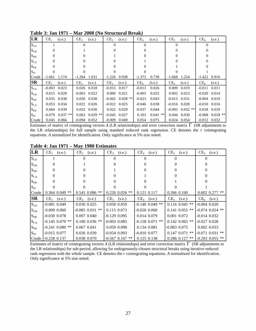
The results of the first estimation are given in Table 3, while those of the four periods of the
second estimation are given in Tables 4-7. We omit nuisance parameter estimates for brevity.
Estimates of the short-run coefficients are less robust than those of long-run coefficients
to misspecification of the number of lags. The robustness of the long-run estimates comes from
the well-known superconsistency of the respective estimators, which may overcome asymptotic
bias from this type of misspecification. Since the short-run estimates have only root-T
convergence in a correctly specified model, they are more sensitive to misspecification of the
stationary covariates (such as number of lagged differences). Since common practice for any
vector time series model is to restrict the number of lags to be the same for every series,
superfluous lags in some series may render short-run coefficients insignificant, while omitted
lags in another series may switch the sign of the estimate.
Note that positive estimates of the non-unit, non-zero elements of the cointegrating
matrix denote negative long-run relationships, and vice versa.
18
5.1 January 1971 – March 2008 (No Breaks)
Allowing no structural breaks does not yield any statistically significant long-run
relationship between stock market and crude oil prices. Moreover, the negative sign is the
opposite of what we expect, suggesting that long-run changes in the crude oil price are
accompanied by long-run changes in stock prices in the same direction. Note that this does not
mean crude oil follows a separate stochastic trend – consistent information criteria suggest only
one common stochastic trend. However, lack of significance clearly indicates uncertainty about
the magnitudes and signs of the cointegrating coefficients.
5.2 January 1971 – May 1980
All estimated long-run parameters during this period have the expected positive sign.
Long-run changes in the crude oil price are therefore accompanied by long-run changes in stock
prices in the opposite direction, as expected. We find these coefficients to be statistically
significant for the U.S., the U.K., Germany, and Italy.
Moreover, a number of the short-run adjustment coefficients are statistically significant.
For example, when Italian stock market is out of equilibrium with the world crude oil price, such
that the Italian stocks are overvalued, statistically significant parameter estimates suggest that the
Italian stock market price should adjust downwards, the crude oil price should adjust downwards,
or the U.K. stock market price should adjust downwards, all else being equal. In fact, if any of
the six stock markets are overvalued relative to the oil price, the respective stock market will
adjust downwards in the short run. However, this relationship is only significant for Italy,
Canada, and the U.K.

19
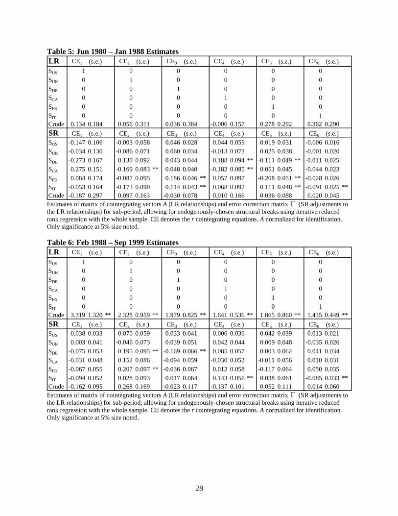
5.3 June 1980 – January 1988
In contrast, none of the long-run relationships are statistically significant during this
period, even though all but Canada have the expected positive sign. Canada is very close to zero,
but the negative sign no doubt results from a precipitous – but perhaps idiosyncratic – decline in
the Canadian stock market during the early part of this period. On the other hand, none are
statistically significantly different from the parameter estimates of the 1971-1980 period,
suggesting the possibility that the structural break in 1980 was limited to the short-run
coefficients.
Without significant long-run relationships, it is difficult to interpret short-run dynamics.
However, a few of them are significant with the correct sign. Similarly to the previous period,
the stock markets adjust downwards in the short-run if overvalued relative to crude oil, except
for Germany. This relationship is significant for Italy, France, and Canada.
5.4 February 1988 – September 1999
During the third period, all of the long-run relationships are significant with the expected
positive sign. This period featured steadily growing stock markets, except for the Italian stock
market around 1992 (probably due to speculative attacks on the Lira at about that time), and
steadily declining oil prices, except during the Gulf War.
Some of the short-run dynamics are significant with the expected sign. Similarly to
previous periods, all of the stock markets adjust downwards in the short-run if overvalued
relative to crude oil, with a significant coefficient for Italy and Germany.
None of the short-run adjustments of the crude oil price to the equilibrium relationships
with stock market prices are significant. The supposed exogeneity of this series may account for
this result. The Italian stock market, for example, would more reasonably adjust downwards to

20
correct an imbalance with the world oil price than would the world oil price adjust downwards to
correct the imbalance.
5.5 September 1999 – May 2008
During the last period, the long-run relationships are mostly insignificant, with the U.S.
and Canada having the wrong sign. The counter-intuitive sign for Canada is even significant.
Even the positive coefficients are substantially smaller than in the previous period. These results
suggest a break in 1999 so substantial that the natural, prevailing long-run relationship fell apart
or was even reversed.
5. Concluding Remarks
We analyze the long-run relationship between the world price of crude oil and
international stock markets over the period from January 1971 to March 2008. We utilize a
cointegrated vector error correction model with additional macroeconomic variables as
regressors to capture short-term influences. Our technique allows for endogenously identified
structural breaks in the cointegrating matrix and error correction matrix.
We find a clear long-run relationship between real stock prices for six OECD countries
and world real oil price from January 1971 until May 1980 and again from February 1988 and
September 19998, with positive statistically significant cointegrating coefficients for real stock
market prices and the real oil price. Intuitively, this means stock market prices increase as the oil
price decrease or decrease as the oil price increase, over the long-run. These results are natural in
light of modern economies’ reliance on oil at all levels of economic activity.
Between May 1980 and February 1988, the relationship is no longer significant. It should
be noted, however, that although these estimates are not statistically significantly different from
zero, neither are they statistically significantly different from the estimates of the previous period.

21
After September 1999, a more substantial break is apparent, with even a sign reversal in
some cases. Overall, the stability of the long-run relationship between crude oil and stock market
prices over the pre-1999 period with the subsequent disintegration or reversal of this relationship
suggests that stock markets have not responded to oil prices in the expected way since then. Such
an empirical finding supports a conjecture of change in the relationship between real oil price
and real stock prices in the last decade compared to earlier years and the presence of several
stock market bubbles and/or oil price bubbles since the turn of the century.

22
References
Ahlgren, N. and J. Antell (2002). ”Testing for Cointegration between International Stock Prices,” Applied Financial Economics, 12, 851-61.
Aznar, A. and M. Salvador (2002). “Selecting the Rank of Cointegration Space and the Form of the Intercept Using an Information Criterion,” Econometric Theory, 18, 926-47.
Barsky, R.B. and L. Kilian (2004). “Oil and the Macroeconomy since the 1970’s,” Journal of Economic Perspectives, 18, 115-34.
Basher, S. A. and P. Sadorsky (2006) “Oil Price Risk and Emerging Stock Markets”, Global Finance Journal, 17, 224-251.
Blanchard, O. J. and J. Gali (2007). “The Macroeconomic Effects of Oil Price Shocks: Why Are 2000’s So Different from the 1970’s?” National Bureau of Economic Research Working Paper 13368.
Boyer, M. M. and D. Filion (2007). “Common and Fundamental Factors in Stock Returns of Canadian Oil and Gas Companies,” Energy Economics, 29, 428-53.
Camarero, M. and C. Tamarit (2002). “Instability Tests in Cointegration Relationships. An Application to the Term Structure of Interest Rates,” Economic Modelling, 19, 783-99.
Chao, J.C. and P.C.B. Phillips (1999). “Model selection in partially nonstationary vector autoregressive processes with reduced rank structure,” Journal of Econometrics, 91, 227-71
Chen, N. F., Roll, R., and S.A. Ross (1986). “Economic Forces and the Stock Market,” Journal of Business, 59, 383-403.
Cheng, X. and P.C.B. Phillips (2008). “Semiparametric Cointegrating Rank Selection,” Discussion Paper 1658, Cowles Foundation.
Ciner, C. (2001). “Energy Shocks and Financial Markets: Nonlinear Linkages.” Studies in Non-Linear Dynamics and Econometrics, 5, 203-12.
Cologni, A. and M. Manera (2008). “Oil prices, inflation and interest rates in a structural cointegrated VAR model for the G-7 countries.” Energy Economics, 30, 856-88.
Cologni, A. and M. Manera (2009). “The Asymmetric Effects of Oil Shocks on Output Growth: A Markov-Switching Analysis for the G-7 Countries,” Economic Modelling, 26, 1-29.
Cunado, J. and F. Perez de Garcia (2005). “Oil Prices, Economic Activity and Inflation: Evidence for Some Asian Countries,” The Quarterly Review of Economics and Finance, 45, 65-83.
El-Sharif, I., D. Brown, B. Burton, B. Nixon, and A. Russell (2005). “Evidence on the Nature and Extent of the Relationship between Oil Prices and Equity Values in the UK.” Energy Economics, 27, 819-30.
Forbes, K. J., and R. Rigobon (2002). “No Contagion, Only Interdependence: Measuring Stock Market Comovements,” The Journal of Finance, 57, 2223-2261.
Gogineni, S. (2007). “The Stock Market Reaction to Oil Price Changes,” Working Paper, University of Oklahoma.
23
Gonzalo, J. and J.Y. Pitarkis (1998), “Specification via model selection in vector error correction models,” Economics Letters, 60, 321-8.
Gregory, A.W. and B.E. Hansen (1996). “Residual-based Tests for Cointegration in Models with Regime Shifts,” Journal of Econometrics, 70, 99-126.
Gronwald, M. (2008). “Large oil shocks and the US economy: Infrequent incidents with large effects,” Energy Journal, 29, 151-71.
Hamilton, J.D. (1983). “Oil and the Macroeconomy since World War II,” Journal of Political Economy, 91, 228-48.
Hamilton, J.D. (1996). “This is What Happened to the Oil Price-Macroeconomy Relationship,” Journal of Monetary Economics, 38, 215-20.
Hamilton, J. D. (2003). “What is an Oil Shock?” Journal of Econometrics, 113, 363-98.
Hansen, H., and S. Johansen (1993). “Recursive Estimation in Cointegrated VAR Models,” mimeograph, Institute of Mathematical Statistics, University of Copenhagen.
Hooker, M.A. (1996). “What Happened to the Oil Price-Macroeconomy Relationship?” Journal of Monetary Economics, 38, 195-213.
Huang, R. D., Masulis, R. W., and H. R. Stoll (1996). “Energy shocks and financial markets,” Journal of Futures Markets, 16, 1-27.
Huntington, H.G. (2005). “The Economic Consequences of Higher Crude Oil Prices,” Energy Modeling Forum, Final Report EMF SR9, Stanford University.
Jimenez-Rodriguez, R. and M. Sanchez (2005). “Oil Price Shocks and Real GDP Growth: Empirical Evidence for Some OECD Countries,” Applied Economics, 37, 201-28.
Johansen, S. (1988). “Statistical Analysis of Cointegration Vectors,” Journal of Economic Dynamics and Control, 12, 231-54.
Johansen, S. (1995). Likelihood-Based Inference on Cointegration in the Vector Autoregressive Model. Oxford: Oxford University Press.
Johansen S., R. Mosconi, and B. Nielsen (2000). “Cointegration Analysis in the Presence of Structural Breaks in the Deterministic Trend,” Journal of Econometrics, 3, 216-49.
Jones, C.M., G. Kaul (1996). “Oil and the Stock Market,” Journal of Finance, 51, 463-91.
Jones, D.W., P.N. Leiby, and I.K. Paik (2004). “Oil Price Shocks and the Macroeconomy: What Has Been Learned Since 1996,” The Energy Journal, 25, 1-32.
Kapetanios, G. (2004). “The Asymptotic Distribution of the Rank Estimator under the Akaike Information Criterion,” Econometric Theory, 20, 735-42.
Kilian, L., and C. Park (2007). “The Impact of Oil Price Shocks on the U.S. Stock Market,” CEPR Discussion Paper No. 6166.
Kilian, L. (2008a). “A Comparison of the Effects of Exogenous Oil Supply Shocks on Output and Inflation in the G7 Countries,” Journal of the European Economic Association, 6, 78-121.
Kilian, L., (2008b). “Exogenous Oil Supply Shocks: How Big Are They and How Much Do They Matter for the US Economy?” Review of Economics and Statistics, 90, 216-40.
24
Korajczyk, R. A. (1996). “A Measure of Stock Market Integration for Developed and Emerging Markets,” World Bank Economic Review, 9, 267-289.
Kwiatkowski, D., P.C.B. Phillips, P. Schmidt, and Y. Shin (1992). “Testing the Null Hypothesis of Stationarity against the Alternative of a Unit Root,” Journal of Econometrics, 54, 159-78.
Lee, B.R., K. Lee, and R.A. Ratti (2001). “Monetary Policy, Oil Price Shocks, and Japanese Economy.” Japan and the World Economy, 13, 321-49.
Lee, K., S. Ni, and R.A. Ratti (1995). “Oil Shocks and the Macroeconomy: The Role of Price Variability,” Energy Journal, 16, 39-56.
Lütkepohl, H., P. Saikkonen, and C. Trenkler (2004). “Testing for the Cointegrating Rank of a VAR Process with Level Shift at Unknown Time,” Econometrica, 72, 647–662.
Mork, K. A. (1989). “Oil and the Macroeconomy When Prices Go Up and Down: An Extension of Hamilton’s Results,” Journal of Political Economy, 97, 740-4.
Nandha, M. and R. Faff (2008). “Does Oil Move Equity Prices? A Global View,” Energy Economics, 30, 986-97.
O’Neill, T.J., J. Penm, and R.D. Terrell (2008). “The Role of Higher Oil Prices: A Case of Major Developed Countries,” Research in Finance, 24, 287-99.
Papapetrou, E. (2001). “Oil Price Shocks, Stock Market, Economic Activity and Employment in Greece,” Energy Economics, 23, 511-32.
Park, J. and R.A. Ratti (2008). “Oil Price Shocks and Stock Markets in the U.S. and 13 European Countries,” Energy Economics, 30, 2587-608.
Phillips, P.C.B, and P. Perron (1988). “Testing for a Unit Root in Time Series Regressions,” Biometrika, 75, 335-46.
Sadorsky, P. (1999). “Oil Price Shocks and Stock Market Activity,” Energy Economics, 21, 449-69.
Sadorsky, P. (2001). “Risk Factors in Stock Returns of Canadian Oil and Gas Companies,” Energy Economics, 23, 17-28.
Sadorsky, P. (2006). “Modeling and Forecasting Petroleum Futures Volatility,” Energy Economics, 28, 467-88.
Saikkonen, P. and H. Lütkepohl (2000). “Testing for the Cointegrating Rank of a VAR Process with Structural Shifts,” Journal of Business and Economic Statistics, 18, 451–64.
Wang, Z. and D.A. Bessler (2005). “A Monte Carlo Study on the Selection of Cointegrating Rank Using Information Criteria,” Econometric Theory, 21, 593-620.

25
Appendix: Data Sources
Data are monthly from January 1971 through March 2008. We construct a single world
real crude oil price by subtracting the log of the U.S. PPI for all commodities from the log of the
nominal price of U.K. Brent (a U.S. dollar index). Real stock market prices for six countries, CA,
FR, DE, IT, UK and US, are created in a similar way using the respective countries’ CPIs. We
also use the log of 100 plus nominal short-term interest rates and the log of real industrial
production for each country. All series are normalized so that the initial values are zero.
The sources of our raw data are as follows:
Nominal Oil Price: U.K. Brent from IFS, International Monetary Fund, (11276AADZF).
Producer Price Index (All Commodities): FRED, FRB of St. Louis (PPIACO).
Stock Market Prices: S&P 500 (US), and Main Economic Indicators, OECD (other countries).
Consumer Price Indices: Main Economic Indicators, OECD.
Industrial Production Indices: Main Economic Indicators, OECD.
Short-term Interest Rates:
US: 3-month Treasury-bill rate from FRED, FRB of St. Louis (TB3MS).
DE: Money market rates reported by Frankfurt banks / Three-month funds / Monthly
average, German Federal Bank.
UK: Treasury bill rate, IFS (line 60c), International Monetary Fund.
IT: money market rate, IFS (line 60c), International Monetary Fund.
FR: money market rate, National Institute for Statistics and Economic Studies (INSEE).
CA: short term rate (three month maturity), OECD.

26
Table 1: Diagnostic Tests on the Individual Series
Int (s.e.) (c.v.) -14.1 -2.86 0.463ΔSUS 0.0025 0.0017 SUS 0.221 -0.093 7.728 **ΔSUK 0.0018 0.0022 SUK -1.199 -0.909 7.197 **ΔSDE 0.0021 0.0025 SDE -1.671 -0.890 7.175 **ΔSCA 0.0020 0.0022 SCA -1.280 -0.570 6.397 **ΔSFR 0.0022 0.0027 SFR -0.979 -0.654 7.204 **ΔSIT 0.0003 0.0028 SIT -2.505 -1.391 4.390 **ΔCrude 0.0047 0.0045 Crude -10.147 -2.393 0.811 **
Z(c) Z(t) KPSSt-tests
Int: Intercept estimate from a first-order autoregression of first differenced series; Z(c) and Z(t): Phillips-Perron unit root coefficient tests and t-tests (unit root null, intercept only); and KPSS: KPSS unit root tests (stationary null, intercept only). Only significance at 5% size noted. Table 2: Information Criteria for Rank and Lag Selection Rank Lag
0 -43.214 -44.490 -43.852 1 -43.249 -43.583 -43.4161 -43.263 -44.575 -43.919 2 -43.599 ** -44.068 -43.8332 -43.276 -44.619 -43.947 3 -43.539 -44.143 -43.8413 -43.283 -44.651 -43.967 4 -43.494 -44.233 -43.8634 -43.284 -44.672 -43.978 5 -43.429 -44.305 -43.8675 -43.286 -44.687 -43.987 6 -43.402 -44.414 -43.9086 -43.287 ** -44.696 ** -43.992 ** 7 -43.343 -44.493 -43.9187 -43.283 -44.695 -43.989 8 -43.360 -44.648 -44.004
9 -43.325 -44.752 -44.03910 -43.235 -44.801 -44.01811 -43.165 -44.871 -44.01812 -43.115 -44.962 -44.03813 -43.080 -45.067 -44.07414 -43.070 -45.199 -44.13415 -43.017 -45.289 -44.153 **16 -42.928 -45.343 ** -44.136
IC3(r) IC2(q) IC3(q)IC1(q)IC1(r) IC2(r)
Information criterion for rank selection (left panel) and lag selection (right panel). Information criteria calculated as IC1(r): Average of HQ across all lags q for rank r; IC2(r): Average of lnHQ across all lags q for rank r; IC3(r): Average of both HQ and lnHQ across all lags q for rank r; IC1(q): Average of HQ across all ranks r for lag q; IC2(q): Average of lnHQ across all ranks r for lag q; and IC3(q): Average of both HQ and lnHQ across all ranks r for lag q. Minimal criterion in each column noted with two asterisks.
27
Table 3: Jan 1971 – Mar 2008 (No Structural Break) LR CE1 (s.e.) CE2 (s.e.) CE3 (s.e.) CE4 (s.e.) CE5 (s.e.) CE6 (s.e.)SUS 1 0 0 0 0 0SUK 0 1 0 0 0 0SDE 0 0 1 0 0 0SCA 0 0 0 1 0 0SFR 0 0 0 0 1 0SIT 0 0 0 0 0 1Crude -1.661 1.174 -1.284 1.031 -1.226 0.938 -1.373 0.738 -1.668 1.254 -1.422 0.916SR CE1 (s.e.) CE2 (s.e.) CE3 (s.e.) CE4 (s.e.) CE5 (s.e.) CE6 (s.e.)SUS -0.003 0.023 0.026 0.018 -0.015 0.017 -0.013 0.026 0.009 0.019 -0.011 0.011SUK 0.015 0.028 -0.003 0.022 0.000 0.021 -0.003 0.032 0.002 0.023 -0.020 0.014SDE 0.035 0.038 0.050 0.030 -0.062 0.028 ** -0.023 0.043 -0.013 0.031 -0.004 0.019SCA 0.053 0.034 0.022 0.026 -0.022 0.025 -0.046 0.038 -0.016 0.028 -0.010 0.016SFR 0.064 0.039 0.032 0.030 0.022 0.029 -0.037 0.044 -0.093 0.032 ** 0.018 0.019SIT -0.079 0.037 ** 0.063 0.029 ** -0.045 0.027 0.103 0.041 ** 0.044 0.030 -0.068 0.018 **Crude 0.045 0.066 -0.094 0.052 -0.009 0.049 0.054 0.075 0.024 0.054 -0.012 0.032Estimates of matrix of cointegrating vectors A (LR relationships) and error correction matrix Γ (SR adjustments to the LR relationships) for full sample using standard reduced rank regression. CE denotes the r cointegrating equations. A normalized for identification. Only significance at 5% size noted. Table 4: Jan 1971 – May 1980 Estimates LR CE1 (s.e.) CE2 (s.e.) CE3 (s.e.) CE4 (s.e.) CE5 (s.e.) CE6 (s.e.)SUS 1 0 0 0 0 0SUK 0 1 0 0 0 0SDE 0 0 1 0 0 0SCA 0 0 0 1 0 0SFR 0 0 0 0 1 0SIT 0 0 0 0 0 1Crude 0.364 0.049 ** 0.545 0.086 ** 0.226 0.026 ** 0.121 0.117 0.266 0.160 0.602 0.277 **SR CE1 (s.e.) CE2 (s.e.) CE3 (s.e.) CE4 (s.e.) CE5 (s.e.) CE6 (s.e.)SUS -0.081 0.049 0.030 0.025 0.058 0.059 -0.140 0.049 ** 0.116 0.045 ** -0.004 0.020SUK 0.009 0.060 -0.085 0.031 ** 0.115 0.073 -0.026 0.060 0.141 0.055 ** -0.074 0.024 **SDE -0.030 0.078 0.007 0.040 -0.129 0.095 0.014 0.079 0.001 0.072 -0.014 0.032SCA -0.145 0.070 ** 0.100 0.036 ** -0.003 0.085 -0.158 0.071 ** 0.142 0.065 ** -0.027 0.028SFR -0.241 0.080 ** 0.067 0.041 0.059 0.098 0.134 0.081 -0.083 0.075 0.002 0.033SIT -0.015 0.077 0.026 0.039 -0.054 0.093 -0.010 0.077 0.147 0.071 ** -0.071 0.031 **Crude -0.228 0.137 0.038 0.070 -0.567 0.167 ** 0.125 0.138 0.286 0.127 ** -0.203 0.055 **Estimates of matrix of cointegrating vectors A (LR relationships) and error correction matrix Γ (SR adjustments to the LR relationships) for sub-period, allowing for endogenously-chosen structural breaks using iterative reduced rank regression with the whole sample. CE denotes the r cointegrating equations. A normalized for identification. Only significance at 5% size noted.
28
Table 5: Jun 1980 – Jan 1988 Estimates LR CE1 (s.e.) CE2 (s.e.) CE3 (s.e.) CE4 (s.e.) CE5 (s.e.) CE6 (s.e.)SUS 1 0 0 0 0 0SUK 0 1 0 0 0 0SDE 0 0 1 0 0 0SCA 0 0 0 1 0 0SFR 0 0 0 0 1 0SIT 0 0 0 0 0 1Crude 0.134 0.184 0.056 0.311 0.036 0.384 -0.006 0.157 0.278 0.292 0.362 0.290SR CE1 (s.e.) CE2 (s.e.) CE3 (s.e.) CE4 (s.e.) CE5 (s.e.) CE6 (s.e.)SUS -0.147 0.106 -0.003 0.058 0.046 0.028 0.044 0.059 0.019 0.031 -0.006 0.016SUK -0.034 0.130 -0.086 0.071 0.060 0.034 -0.013 0.073 0.025 0.038 -0.001 0.020SDE -0.273 0.167 0.130 0.092 0.043 0.044 0.188 0.094 ** -0.111 0.049 ** -0.011 0.025SCA 0.275 0.151 -0.169 0.083 ** 0.048 0.040 -0.182 0.085 ** 0.051 0.045 -0.044 0.023SFR 0.084 0.174 -0.087 0.095 0.186 0.046 ** 0.057 0.097 -0.208 0.051 ** -0.028 0.026SIT -0.053 0.164 -0.173 0.090 0.114 0.043 ** 0.068 0.092 0.111 0.048 ** -0.091 0.025 **Crude -0.187 0.297 0.097 0.163 -0.030 0.078 0.010 0.166 0.036 0.088 0.020 0.045Estimates of matrix of cointegrating vectors A (LR relationships) and error correction matrix Γ (SR adjustments to the LR relationships) for sub-period, allowing for endogenously-chosen structural breaks using iterative reduced rank regression with the whole sample. CE denotes the r cointegrating equations. A normalized for identification. Only significance at 5% size noted. Table 6: Feb 1988 – Sep 1999 Estimates LR CE1 (s.e.) CE2 (s.e.) CE3 (s.e.) CE4 (s.e.) CE5 (s.e.) CE6 (s.e.)SUS 1 0 0 0 0 0SUK 0 1 0 0 0 0SDE 0 0 1 0 0 0SCA 0 0 0 1 0 0SFR 0 0 0 0 1 0SIT 0 0 0 0 0 1Crude 3.319 1.320 ** 2.328 0.959 ** 1.979 0.825 ** 1.641 0.536 ** 1.865 0.860 ** 1.435 0.449 **SR CE1 (s.e.) CE2 (s.e.) CE3 (s.e.) CE4 (s.e.) CE5 (s.e.) CE6 (s.e.)SUS -0.038 0.033 0.070 0.059 0.033 0.041 0.006 0.036 -0.042 0.039 -0.013 0.021SUK 0.003 0.041 -0.046 0.073 0.039 0.051 0.042 0.044 0.009 0.048 -0.035 0.026SDE -0.075 0.053 0.195 0.095 ** -0.169 0.066 ** 0.085 0.057 0.003 0.062 0.041 0.034SCA -0.031 0.048 0.152 0.086 -0.094 0.059 -0.030 0.052 -0.011 0.056 0.010 0.031SFR -0.067 0.055 0.207 0.097 ** -0.036 0.067 0.012 0.058 -0.117 0.064 0.050 0.035SIT -0.094 0.052 0.028 0.093 0.017 0.064 0.143 0.056 ** 0.038 0.061 -0.085 0.033 **Crude -0.162 0.095 0.268 0.169 -0.023 0.117 -0.137 0.101 0.052 0.111 0.014 0.060Estimates of matrix of cointegrating vectors A (LR relationships) and error correction matrix Γ (SR adjustments to the LR relationships) for sub-period, allowing for endogenously-chosen structural breaks using iterative reduced rank regression with the whole sample. CE denotes the r cointegrating equations. A normalized for identification. Only significance at 5% size noted.

29
Table 7: Oct 1999 – Mar 2008 Estimates LR CE1 (s.e.) CE2 (s.e.) CE3 (s.e.) CE4 (s.e.) CE5 (s.e.) CE6 (s.e.)SUS 1 0 0 0 0 0SUK 0 1 0 0 0 0SDE 0 0 1 0 0 0SCA 0 0 0 1 0 0SFR 0 0 0 0 1 0SIT 0 0 0 0 0 1Crude -0.078 0.433 0.196 0.572 0.036 0.555 -0.410 0.151 ** 0.138 0.665 0.007 0.296SR CE1 (s.e.) CE2 (s.e.) CE3 (s.e.) CE4 (s.e.) CE5 (s.e.) CE6 (s.e.)SUS -0.065 0.087 0.150 0.125 -0.084 0.057 0.075 0.081 -0.024 0.109 -0.011 0.069SUK 0.036 0.107 0.046 0.153 -0.073 0.070 -0.007 0.100 -0.026 0.133 0.056 0.084SDE 0.041 0.136 0.948 0.194 ** -0.289 0.089 ** 0.316 0.127 ** -0.750 0.169 ** 0.218 0.107 **SCA 0.044 0.126 0.317 0.179 0.005 0.082 -0.005 0.117 -0.319 0.156 ** 0.046 0.099SFR -0.071 0.143 0.568 0.204 ** -0.051 0.093 0.201 0.133 -0.430 0.177 ** -0.005 0.112SIT -0.118 0.135 0.359 0.193 -0.028 0.088 0.163 0.126 -0.207 0.168 -0.094 0.106Crude 0.342 0.242 -0.168 0.345 0.065 0.158 0.462 0.225 ** -0.078 0.300 -0.326 0.190Estimates of matrix of cointegrating vectors A (LR relationships) and error correction matrix Γ (SR adjustments to the LR relationships) for sub-period, allowing for endogenously-chosen structural breaks using iterative reduced rank regression with the whole sample. CE denotes the r cointegrating equations. A normalized for identification. Only significance at 5% size noted.