Cross-correlation-based image acquisition...

Cross-correlation-based image acquisition

technique for manually-scanned optical

coherence tomography

Adeel Ahmad1, Steven G. Adie

1, Eric J. Chaney

1, Utkarsh Sharma

1,

and Stephen A. Boppart*1, 2

Biophotonics Imaging Laboratory

Beckman Institute for Advanced Science and Technology 1 Department of Electrical and Computer Engineering,

2 Department of Bioengineering, Department of Medicine

University of Illinois at Urbana-Champaign

405 N. Mathews Avenue, Urbana, IL 61801 *Corresponding author: [email protected]

Abstract: We present a novel image acquisition technique for Optical

Coherence Tomography (OCT) that enables manual lateral scanning. The

technique compensates for the variability in lateral scan velocity based on

feedback obtained from correlation between consecutive A-scans. Results

obtained from phantom samples and biological tissues demonstrate

successful assembly of OCT images from manually-scanned datasets

despite non-uniform scan velocity and abrupt stops encountered during data

acquisition. This technique could enable the acquisition of images during

manual OCT needle-guided biopsy or catheter-based imaging, and for

assembly of large field-of-view images with hand-held probes during

intraoperative in vivo OCT imaging.

2009 Optical Society of America

OCIS codes: (170.4500) Optical coherence tomography; (120.5800) Scanners

References and links

1. D. Huang, E. A. Swanson, C. P. Lin, J. S. Schuman, W. G. Stinson, W. Chang, M. R. Hee, T. Flotte, K.

Gregory, C. A. Puliafito, and J. G. Fujimoto, "Optical coherence tomography," Science 254, 1178-1181

(1991).

2. W. Drexler, and J. G. Fujimoto, Optical coherence tomography: technology and applications ( Springer,

New York 2008).

3. A. M. Zysk, F. T. Nguyen, A. L. Oldenburg, D. L. Marks, and S. A. Boppart, "Optical coherence

tomography: a review of clinical development from bench to bedside," J. Biomed. Opt 12, 051403-051421

(2007).

4. R. Huber, M. Wojtkowski, and J. G. Fujimoto, "Fourier domain mode locking (FDML): A new laser

operating regime and applications for optical coherence tomography," Opt. Express 14, 3225-3237 (2006).

5. Z. Chen, Z. Yonghua, S. M. Srinivas, J. S. Nelson, N. Prakash, and R. D. Frostig, "Optical Doppler

tomography," IEEE J. Sel. Top. Quantum Electron. 5, 1134-1142 (1999).

6. J. J. Pasquesi, S. C. Schlachter, M. D. Boppart, E. J. Chaney, S. J. Kaufman, and S. A. Boppart, "In vivo

detection of exercise-induced ultrastructural changes in genetically-altered murine skeletal muscle using

polarization-sensitive optical coherence tomography," Opt. Express 14, 1547-1556 (2006).

7. A. L. Oldenburg, V. Crecea, S. A. Rinne, and S. A. Boppart, "Phase-resolved magnetomotive OCT for

imaging nanomolar concentrations of magnetic nanoparticles in tissues," Opt. Express 16, 11525-11539

(2008).

8. S. A. Boppart, W. Luo, D. L. Marks, and K. W. Singletary, "Optical coherence tomography: feasibility for

basic research and image-guided surgery of breast cancer," Breast Cancer Res. Treatment 84, 85-97 (2004).

9. S. Radhakrishnan, A. M. Rollins, J. E. Roth, S. Yazdanfar, V. Westphal, D. S. Bardenstein, and J. A. Izatt,

"Real-time optical coherence tomography of the anterior segment at 1310 nm," Arch. Ophthalmol. 119,

1179-1185 (2001).

10. F. I. Feldchtein, V. M. Gelikonov, and G. V. Gelikonov, "Design of OCT scanners" in Handbook of optical

coherence tomography (Marcel Dekker, Inc, 2002).

(C) 2009 OSA 11 May 2009 / Vol. 17, No. 10 / OPTICS EXPRESS 8125#109082 - $15.00 USD Received 23 Mar 2009; revised 20 Apr 2009; accepted 21 Apr 2009; published 29 Apr 2009

11. X. Li, C. Chudoba, T. Ko, C. Pitris, and J. G. Fujimoto, "Imaging needle for optical coherence

tomography," Opt. Lett. 25, 1520-1522 (2000).

12. S. A. Boppart, B. E. Bouma, C. Pitris, G. J. Tearney, J. G. Fujimoto, and M. E. Brezinski, "Forward-

imaging instruments for optical coherence tomography," Opt. Lett. 22, 1618-1620 (1997).

13. S. Han, M. V. Sarunic, J. Wu, M. Humayun, and C. Yang, "Handheld forward-imaging needle endoscope

for ophthalmic optical coherence tomography inspection," J. Biomed. Opt 13, 020505 (2008).

14. P. Cinquin, E. Bainville, C. Barbe, E. Bittar, V. Bouchard, I. Bricault, G. Champleboux, M. Chenin, L.

Chevalier, Y. Delnondedieu, L. Desbat, V. Dessenne, A. Hamadeh, D. Henry, N. Laieb, S. Lavallee, J. M.

Lefebvre, F. Leitner, Y. Menguy, F. Padieu, O. Peria, A. Poyet, M. Promayon, S. Rouault, P. Sautot, J.

Troccaz, and P. Vassal, "Computer assisted medical interventions," IEEE. Eng. Med. Biol. Mag 14, 254-

263 (1995).

15. R. L. Galloway, "The process and development of image guided procedures," Annu. Rev. Biomed. Eng 3,

83-108 (2001).

16. A. H. Gee, R. James Housden, P. Hassenpflug, G. M. Treece, and R. W. Prager, "Sensorless freehand 3D

ultrasound in real tissue: Speckle decorrelation without fully developed speckle," Med. Image Anal 10,

137-149 (2006).

17. L. Mercier, T. Langø, F. Lindseth, and D. L. Collins, "A review of calibration techniques for freehand 3-D

ultrasound systems," Ultrasound Med. Biol 31, 449-471 (2005).

18. P. Hassenpflug, R. W. Prager, G. M. Treece, and A. H. Gee, "Speckle classification for sensorless freehand

3-D ultrasound," Ultrasound Med. Biol 31, 1499-1508 (2005).

19. T. A Tuthill, J. F. Krucker, J. B. Fowlkes, and P. L. Carson, "Automated three-dimensional US frame

positioning computed from elevational speckle decorrelation," Radiology 209, 575-582 (1998).

20. L. Pai-Chi, C. Chong-Jing, and Y. Chih-Kuang, "On velocity estimation using speckle decorrelation "

IEEE. Trans. Ultrason. Ferroelectr. Freq. Control 48, 1084-1091 (2001).

21. R. W. Prager, A. H. Gee, G. M. Treece, C. J. C. Cash, and L. H. Berman, "Sensorless freehand 3-D

ultrasound using regression of the echo intensity," Ultrasound Med. Biol 29, 437-446 (2003).

22. A. Krupa, G. Fichtinger, and G. D. Hager, "Full Motion Tracking in Ultrasound Using Image Speckle

Information and Visual Servoing," in Proceedings of IEEE International Conference on Robotics and

Automation (2007), pp. 2458-2464.

23. P. C. Li, C. Y. Li, and W. C. Yeh, "Tissue motion and elevational speckle decorrelation in freehand 3D

ultrasound," Ultrason. Imaging 24, 1-12 (2002).

24. K. W. Gossage, T. S. Tkaczyk, J. J. Rodriguez, and J. K. Barton, "Texture analysis of optical coherence

tomography images: feasibility for tissue classification," J. Biomed. Opt 8, 570-575 (2003).

25. S. J. Kirkpatrick, R. K. Wang, and D. D. Duncan, "OCT-based elastography for large and small

deformations," Opt. Express 14, 11585-11597 (2006).

26. D. D. Duncan, and S. J. Kirkpatrick, "Processing algorithms for tracking speckle shifts in optical

elastography of biological tissues," J. Biomed. Opt 6, 418-426 (2001).

27. D. D. Duncan, and S. J. Kirkpatrick, "Performance analysis of a maximum-likelihood speckle motion

estimator," Opt. Express 10, 927-941 (2002).

28. H.-J. Ko, W. Tan, R. Stack, and S. A. Boppart, "Optical coherence elastography of engineered and

developing tissue," Tissue Eng 12, 63-73 (2006).

29. S. H. Yun, G. J. Tearney, J. F. de Boer, and B. E. Bouma, "Motion artifacts in optical coherence

tomography with frequency-domain ranging," Opt. Express 12, 2977-2998 (2004).

30. R. J. Zawadzki, S. S. Choi, S. M. Jones, S. S. Oliver, and J. S. Werner, "Adaptive optics-optical coherence

tomography: optimizing visualization of microscopic retinal structures in three dimensions," J. Opt. Soc.

Am. A 24, 1373-1383 (2007).

31. J. M. Schmitt, S. H. Xiang, and K. M. Yung, "Speckle in optical coherence tomography," J. Biomed. Opt 4,

95-105 (1999).

32. W. Luo, D. L. Marks, T. S. Ralston, and S. A. Boppart, "Three-dimensional optical coherence tomography

of the embryonic murine cardiovascular system," J. Biomed. Opt 11, 021014-021018 (2006).

33. A. M. Zysk, and S. A. Boppart, "Computational methods for analysis of human breast tumor tissue in

optical coherence tomography images," J. Biomed. Opt 11, 054015 (2006).

34. M. Wojtkowski, V. J. Srinivasan, T. H. Ko, J. G. Fujimoto, A. Kowalczyk, and J. S. Duker, "Ultrahigh-

resolution, high-speed, fourier domain optical coherence tomography and methods for dispersion

compensation," Opt. Express 12, 2404-2422 (2004).

35. R. J. Housden, A. H. Gee, R. W. Prager, and G. M. Treece, "Rotational motion in sensorless freehand three-

dimensional ultrasound," Ultrasonics 48, 412-422 (2008).

36. R. J. Housden, A. H. Gee, G. M. Treece, and R. W. Prager, "Subsample interpolation strategies for

sensorless freehand 3D ultrasound," Ultrasound Med. Biol 32, 1897-1904 (2006).

1. Introduction

Optical coherence tomography (OCT) is a non-invasive optical imaging technique which

measures backscattered light to provide high resolution (1-10µm) cross-sectional or three


dimensional images of biological tissues [1]. The OCT technology has undergone significant

advances in instrumentation that has expanded its clinical applications [2, 3]. The

development of Fourier-domain acquisition methods have made it possible to acquire real-

time in vivo images with enhanced sensitivity and high scan rates [4], and various structural,

functional and molecular contrast enhancing methods such as Doppler OCT, polarization-

sensitive OCT, spectroscopic OCT, and magnetomotive OCT have further extended the range

of possible applications of OCT [5-7].

One of the major advantages of OCT is that it provides real-time non-invasive diagnostic

feedback about microscopic tissue architecture. This information, for example, is useful to

physicians to assist them in making real-time decisions during time-sensitive diagnostic and

surgical procedures such as needle biopsy, minimally-invasive surgery or procedures, or the

removal of tumor tissue [8]. Despite the real-time, high-resolution imaging capabilities of

OCT, the feasibility and success of implementing OCT in clinical and intraoperative

conditions may largely be determined by the adaptability of OCT instrumentation and image

acquisition techniques to make it more ‘surgeon friendly’. While real-time portable OCT

systems have been successfully demonstrated for clinical research over the last few years [9],

the technology has yet to evolve towards providing an imaging capability that can be readily

used by physicians under the diverse set of conditions encountered in an operating room.

Conventionally, in OCT imaging of tissue specimens or pre-clinical models, the specimen

is placed on a fixed stage and an OCT image is acquired by sequential acquisition of depth-

resolved A-scans synchronized with the lateral scanning of the beam using the computer-

controlled motion of galvanometer-mounted mirrors. While this method provides excellent

accuracy, the lateral scan range is limited by the limited angular range of the galvanometer

and the finite aperture of the objective lens. Although using larger diameter objective lenses

could enhance the scan range, they add to the bulk of the sample arm, which is even more

problematic for hand-held mechanically-scanning probes. An alternative approach to obtain

larger field-of-view is to keep the sample arm beam fixed and translate the sample at a

uniform velocity using a stepper motor controlled stage. Clearly this method is impractical for

in vivo OCT imaging applications, and the translation rate is slow. Various hand-held scanners

and needle-based beam delivery systems have been reported which can provide more

convenient access to tissues and organs in a clinical environment. Most of these scanners have

a means for lateral scanning within the probe head [10-13]. However, these mechanisms make

the probe more complicated, bulky, and expensive. Mechanical scanning mechanisms also

frequently need to be customized for specific in vivo and intraoperative OCT imaging

applications while still providing limited flexibility in choosing the scanning geometries. The

added complexity and cost due to customized designs could make OCT a less attractive option

for a number of applications.

In many circumstances, a surgeon might prefer to use a simple hand-held manually-

scanned probe to obtain OCT images of tissues and organs which might otherwise be

inaccessible using standard mechanically-scanning probes. However, manually scanning a

hand-held probe can cause a number of image artifacts due to variations in the scan velocity

and orientation of the probe. Consequently, image formation with a manually-scanning probe

requires a method to synchronize the acquired A-scans with the relative displacement between

the sample and probe. Methods similar to position tracking of surgical instruments in image-

guided surgical systems can be used for this purpose [14]. These systems attach reference

markers to the probe that are commonly sensed by optical or magnetic field sensors. The

position of these reference markers is tracked by cameras or other suitable sensing systems,

allowing compensation for the relative movement between the sample and the probe [15].

Despite their popularity, the use of an external position sensor is not ideal as it imposes a

number of constraints on image acquisition. These sensors have to be carefully calibrated,

typically have sub-millimeter spatial resolution, and the operating distances need to be within

the range of the mounted sensor and the base unit. For sensors based on optics, a clear line of


sight must be maintained [16], while magnetic field-based sensing systems are highly

susceptible to electromagnetic interference [17].

Clearly, position tracking without the use of an external position sensor can offer

significant advantages. The challenge, however, is to utilize the acquired data or images to

deduce precise motion estimation. Sensorless freehand scanning using speckle decorrelation

has been extensively studied in ultrasound [18, 19]. Speckle decorrelation methods have been

used in ultrasound for velocity estimation [20], 3-D ultrasound [21], and motion tracking [22]

with varying success. One study reported that accurate displacement estimation in sensorless

freehand ultrasound is not possible using speckle decorrelation methods alone [23]. In optics,

speckle patterns have been used for image analysis [24] and elastography [25]. Motion artifact

correction, tissue elastography, and blood velocity measurements in OCT all rely heavily on

motion estimation techniques [25-29]. Algorithms based on 2-D cross-correlations of B-mode

OCT images have been used in tissue elastography [25] and motion artifact correction [30].

In this paper we present a novel technique for the acquisition of manually-scanned OCT

images based on the cross-correlation of A-scans within a 2-D OCT image. This method not

only provides a simpler and less expensive scanning solution with an extended field-of-view,

but also allows greater flexibility and freedom of movement while acquiring OCT images.

The focus of this research study is to compensate for the image distortion and inaccuracies

that occur during non-uniform motion of the probe during lateral manual scanning. To the best

of our knowledge, no prior work has been done in applying motion estimation techniques for

image formation in sensorless manual-scanning OCT. In Section 2 we present details of the

cross-correlation algorithm used for image assembly. Section 3 presents typical decorrelation

curves, followed by results of images assembled from manually-scanned tissue phantoms and

biological tissues. We summarize the main findings and significance of this work in Section 4,

followed by conclusions in Section 5.

2. Methods

2.1 Image acquisition algorithm

The algorithm used for image assembly is shown schematically in Fig. 1. An OCT image is a

sequential assembly of uniformly spaced A-scans. Consecutive A-scans within one resolution

volume will have high cross-correlation due to the regions of overlap, depending on the

amount of oversampling of the sample. Oversampling in this context means sampling more

than twice within the transverse resolution of the OCT system, which depends upon both the

transverse resolution of the OCT system and the lateral step size. Due to the high A-scan rates

available with current systems, and to fully reconstruct the features of the sample, OCT

images are usually oversampled. We define the sampling factor ζ for a manually-scanned

system as:

f xs

vζ

∆= (1)

where x∆ is the transverse resolution of the OCT system which is equal to the diameter of the

beam (1/e2 intensity) at the focus in the sample arm,

sf is the A-scan acquisition rate (Hz) and

v is the velocity of the moving sample or probe. A value of ζ < 2 indicates undersampling and

ζ > 2 oversampling. Note that sampling at the Nyquist rate occurs when ζ = 2.

Non-uniform movement of the probe will cause non-uniform sampling of the sample

which in turn causes variability in the cross-correlation between adjacent A-scans. While

slower scan velocities will result in sequential A-scans with higher correlation, faster scan

velocities will result in reduced correlation between successive A-scans. The maximum

velocity with which the probe or sample can move relative to each other to prevent

undersampling is determined when ζ = 2 in Eq. (1). The goal of the algorithm presented here

is to discard all oversampled regions of a manually-scanned image, essentially reconstructing


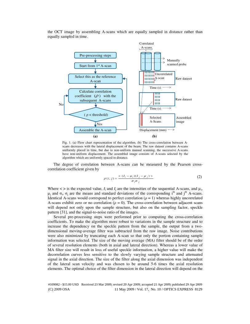
the OCT image by assembling A-scans which are equally sampled in distance rather than

equally sampled in time.

Raw dataset

Correlated

A-scans

Manually

scanned probe

Uncorrelated

A-scan

Start from 1st A-scan

Calculate correlation

coefficient ( ) with the

subsequent A-scans

( ρ < threshold)

Yes

No

Select this as the reference

A-scan

Pre-processing steps

Assemble the A-scan

ρ

(a) (b)

Time (s)

Displacement (mm)

Raw dataset

Assembled

image

Selected

A-Scans

Time (s)

Fig. 1. (a) Flow chart representation of the algorithm. (b) The cross-correlation between A-

scans decreases with the lateral displacement of the beam. The raw dataset contains A-scans

uniformly placed in time, but due to non-uniform manual scanning, the successive A-scans

have non-uniform displacement. The assembled image consists of A-scans selected by the

algorithm which are uniformly spaced in distance.

The degree of correlation between A-scans can be measured by the Pearson cross-

correlation coefficient given by

( ) ( )( , )

i i j j

i j

I Ii j

µ µρ

σ σ

< − − >=

(2)

Where < > is the expected value, Ii and Ij are the intensities of the sequential A-scans, and µ i,

µ j and σi, σj are the means and standard deviations of the corresponding ith

and jth

A-scans.

Identical A-scans would correspond to perfect correlation (ρ = 1) whereas highly uncorrelated

A-scans exhibit zero or no correlation (ρ = 0). The cross-correlation between adjacent scans

will depend not only upon the sample structure, but also on the sampling factor, speckle

pattern [31], and the signal-to-noise ratio of the images.

Several pre-processing steps were performed prior to computing the cross-correlation

coefficients. To make the algorithm more robust to variations in the sample structure and to

increase the dependency on the speckle pattern from the sample, the output from a two-

dimensional moving-average filter was subtracted from the raw image. Noise contributions

were also minimized by truncating each A-scan so that only the portion containing sample

information was selected. The size of the moving average (MA) filter should be of the order

of several resolution elements (both in axial and lateral direction). Whereas a lower value of

MA filter size will result in loss of useful speckle information, a higher value will make the

decorrelation curves less sensitive to the slowly varying sample structure and attenuated

signal in the axial direction. The size of the filter along the axial dimension was independent

of the lateral scan velocity and was chosen to be around 5-6 times the axial resolution

elements. The optimal choice of the filter dimension in the lateral direction will depend on the


lateral scanned velocity, however when used in conjunction with the axial dimension the

choice of filter size along this direction is less critical.

A decorrelation curve plotted for a sample depicts the decrease in the correlation

coefficient value as a function of lateral displacement between two A-scans. Based on the

decorrelation curve of a sample, a threshold can be determined, corresponding to the desired

sampling factor for the assembled image. The first A-scan is selected as the reference and the

cross-correlation coefficients with the subsequently-acquired A-scans are computed. When

the correlation coefficient falls below the selected threshold, the displacement is deemed to

satisfy the desired sampling criteria, and the A-scan is appended to the assembled image. This

assembled A-scan is now selected as the new reference and the steps are repeated until the

algorithm iterated through all acquired A-scans.

2.2 Experimental setup

Measurements were conducted using the spectral-domain OCT system described previously

[32]. Briefly, a Ti-Sapphire laser with 800 nm center wavelength and 90 nm bandwidth was

used, providing an axial resolution of 5 µm. The power in the sample arm was 10 mW and the

samples were imaged with a 40 mm lens producing a transverse resolution of 16 µm. The

experiments for manual scanning at a larger scan range ~ 1 cm were conducted at a line scan

rate of 1 kHz and an exposure time of 200 µs for the line scan camera. The other remaining

experiments were performed at a line scan rate of 5 kHz. The sensitivity of the system at 1

kHz was measured to be 96 dB. The relatively low scan rate was chosen to allow sufficient

time for manually translating the sample under the fixed OCT beam. The computer-controlled

translational stage axes were aligned with the axes of a manually movable spring-loaded

translational stage in order to obtain OCT images of the same cross-sectional planes within a

sample while employing two different scanning mechanisms.

3. Results

3.1 Decorrelation curves for tissue phantoms and biological tissue

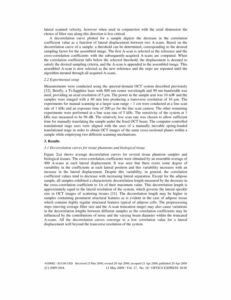
Figure 2(a) shows average decorrelation curves for several tissue phantom samples and

biological tissues. The cross-correlation coefficients were obtained by an ensemble average of

400 A-scans at each lateral displacement. It was seen that there exists some degree of

variability in the coefficients at each lateral position and this variability increases with an

increase in the lateral displacement. Despite this variability, in general, the correlation

coefficient values tend to decrease with increasing lateral separation. Except for the adipose

sample, all samples exhibited a characteristic decorrelation length measured by the decrease in

the cross-correlation coefficient to 1/e of their maximum value. This decorrelation length is

approximately equal to the lateral resolution of the system, which governs the lateral speckle

size in OCT images of scattering tissues [31]. The decorrelation length may be higher in

samples containing prominent structural features as is evident in the case of adipose tissue

which contains highly regular structural features typical of adipose cells. The preprocessing

steps (moving average filter size and the A-scan truncation range) may also cause variations

in the decorrelation lengths between different samples as the correlation coefficients may be

influenced by the contributions of noise and the varying beam diameter within the truncated

A-scans. All the decorrelation curves converge to a low correlation value for a lateral

displacement well beyond the transverse resolution of the system.


Lateral Displacement (µm)

Cro

ss-c

orr

elati

on

Co

effi

cients

Tissue phantomRat adiposePlaticine

Rat intestineHuman skin

1

0.9

0.8

0.7

0.6

0.5

0.4

0.3

0.2

0.1

0

-100 -75 -50 -25 0 25 50 75 100

Fig. 2. Decorrelation curves obtained from galvanometer-scanned images of several tissue

phantom samples and biological tissues (negative distance corresponds to the cross-correlation

between the current A-scan and previously acquired A-scans). The tissue phantom was a

silicone-based sample with titanium dioxide (TiO2) scattering particles.

3.2 Image assembly for a tissue phantom

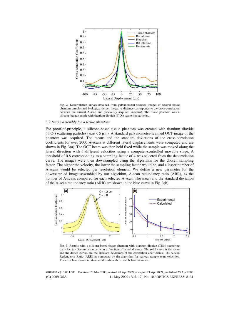
For proof-of-principle, a silicone-based tissue phantom was created with titanium dioxide

(TiO2) scattering particles (size < 5 µm). A standard galvanometer-scanned OCT image of the

phantom was acquired. The means and the standard deviations of the cross-correlation

coefficients for over 2000 A-scans at different lateral displacements were computed and are

shown in Fig. 3(a). The OCT beam was then held fixed while the sample was moved along the

lateral direction with 5 different velocities using a computer-controlled movable stage. A

threshold of 0.8 corresponding to a sampling factor of 4 was selected from the decorrelation

curve. The images were then downsampled using the algorithm for the chosen sampling

factor. The higher the velocity, the lower the sampling factor would be, and a lesser number of

A-scans would be selected per resolution element. We define a new parameter for the

downsampled image assembled by our algorithm, A-scan redundancy ratio (ARR), as the

number of A-scans compared for each selected A-scan. The mean and the standard deviation

of the A-scan redundancy ratio (ARR) are shown in the blue curve in Fig. 3(b).

Lateral Displacement (µm) Velocity (mm/s)

Cro

ss-c

orr

elati

on

Coef

fici

ents

A-S

can R

edund

ancy R

atio

X = 4.2 µmY = 0.8

Experimental

Calculated

-20 0 20 0.5 1 1.5 2 2.5

1

0.8

0.6

0.4

0.2

0

50

40

30

20

10

Fig. 3. Results with a silicone-based tissue phantom with titanium dioxide (TiO2) scattering

particles. (a) Decorrelation curve as a function of lateral distance. The solid curve is the mean

and the dotted curves are the standard deviations of the correlation coefficients. (b) A-scan

Redundancy Ratio (ARR) as computed by the algorithm for various sample scan velocities.

The error bars show one standard deviation above and below the mean.


Equation. (1) was used to calculate the actual sampling factor for different scan velocities

given the A-scan rate of 5 kHz and transverse resolution of 16 µm. The calculated sampling

factor was then divided by the desired sampling factor (equal to 4 in this case) to calculate the

ARR between the raw and assembled image and is plotted as the red dotted curve in Fig. 3(b).

The results show that the experimentally-obtained results are in good agreement with the

numerically-predicted values. The algorithm is able to compensate for variations in scan

velocity by adjusting the periodicity of A-scan selection from the raw image data set. As seen

in Fig. 3(b), the ARR curve is more sensitive to velocity variations for highly oversampled

datasets, suggesting that the algorithm will provide better results for raw images taken with

higher sampling factors. This would occur with slower scanning velocities or with advanced

OCT systems with exceptionally fast A-scan acquisition rates.

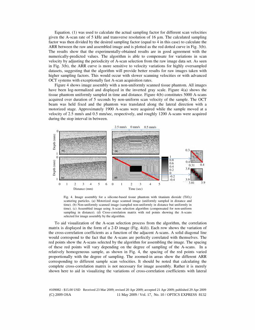
Figure 4 shows image assembly with a non-uniformly scanned tissue phantom. All images

have been log-normalized and displayed in the inverted gray scale. Figure 4(a) shows the

tissue phantom uniformly sampled in time and distance. Figure 4(b) constitutes 5000 A-scans

acquired over duration of 5 seconds by non-uniform scan velocity of the sample. The OCT

beam was held fixed and the phantom was translated along the lateral direction with a

motorized stage. Approximately 1900 A-scans were acquired while the sample moved at a

velocity of 2.5 mm/s and 0.5 mm/sec, respectively, and roughly 1200 A-scans were acquired

during the stop interval in between.

Distance (mm) Time (sec)

0.5 mm/s2.5 mm/s 0 mm/s

(a) (b)

(c) (d)

Dep

th (

mm

)D

epth

(m

m)

0

10

1

0 1 2 3 4 5 6 0 1 2 3 4 5

10.80.60.40.20-0.2-0.4

0.3

0.40.31 0.4

3.8

3.93.81 3.9

Fig. 4. Image assembly for a silicone-based tissue phantom with titanium dioxide (TiO2)

scattering particles. (a) Motorized stage scanned image (uniformly sampled in distance and

time). (b) Non-uniformly scanned image (sampled non-uniformly in distance but uniformly in

time). (c) Assembled image using A-scan selection algorithm (compensated for non-uniform

sampling in distance). (d) Cross-correlation matrix with red points showing the A-scans

selected for image assembly by the algorithm.

To aid visualization of the A-scan selection process from the algorithm, the correlation

matrix is displayed in the form of a 2-D image (Fig. 4(d)). Each row shows the variation of

the cross-correlation coefficients as a function of the adjacent A-scans. A solid diagonal line

would correspond to the fact that the A-scans are perfectly correlated with themselves. The

red points show the A-scans selected by the algorithm for assembling the image. The spacing

of these red points will vary depending on the degree of sampling of the A-scans. In a

relatively homogeneous sample, as shown in Fig. 4, the spacing of the red points varied

proportionally with the degree of sampling. The zoomed-in areas show the different ARR

corresponding to different sample scan velocities. It should be noted that calculating the

complete cross-correlation matrix is not necessary for image assembly. Rather it is merely

shown here to aid in visualizing the variations of cross-correlation coefficients with lateral


displacement, where dark regions correspond to little or no movement and lighter regions

correspond to rapid movements.

Figure 4(c) shows the result after correcting for non-uniform sampling in distance. A

threshold value of 0.7 was used for image assembly corresponding to a sampling factor of 2.

The algorithm selected approximately 580 and 135 A-scans from the regions corresponding to

the velocities 2.5 mm/sec and 0.5 mm/sec, respectively, making the assembled image

uniformly sampled with a sampling factor of 1.95-2.30.

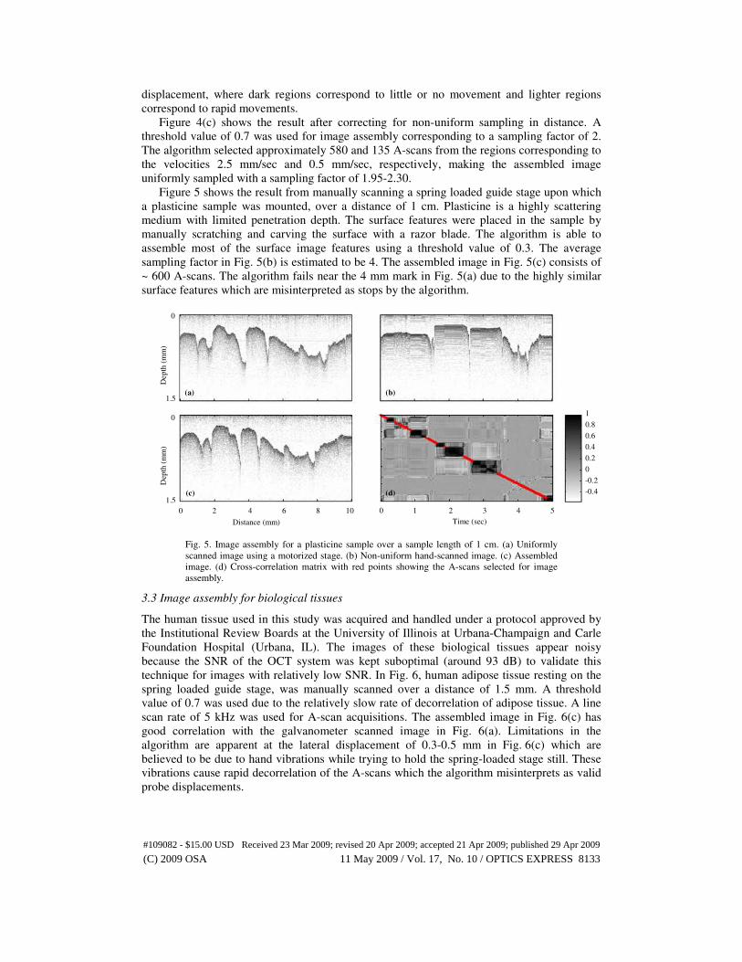
Figure 5 shows the result from manually scanning a spring loaded guide stage upon which

a plasticine sample was mounted, over a distance of 1 cm. Plasticine is a highly scattering

medium with limited penetration depth. The surface features were placed in the sample by

manually scratching and carving the surface with a razor blade. The algorithm is able to

assemble most of the surface image features using a threshold value of 0.3. The average

sampling factor in Fig. 5(b) is estimated to be 4. The assembled image in Fig. 5(c) consists of

~ 600 A-scans. The algorithm fails near the 4 mm mark in Fig. 5(a) due to the highly similar

surface features which are misinterpreted as stops by the algorithm.

Distance (mm)

Depth

(m

m)

Dep

th (

mm

)

0

1.5

0

1.5

(a) (b)

(c) (d)

Time (sec)

0 1 2 3 4 50 2 4 6 8 10

1

0.8

0.6

0.4

0.2

0

-0.2

-0.4

Fig. 5. Image assembly for a plasticine sample over a sample length of 1 cm. (a) Uniformly

scanned image using a motorized stage. (b) Non-uniform hand-scanned image. (c) Assembled

image. (d) Cross-correlation matrix with red points showing the A-scans selected for image

assembly.

3.3 Image assembly for biological tissues

The human tissue used in this study was acquired and handled under a protocol approved by

the Institutional Review Boards at the University of Illinois at Urbana-Champaign and Carle

Foundation Hospital (Urbana, IL). The images of these biological tissues appear noisy

because the SNR of the OCT system was kept suboptimal (around 93 dB) to validate this

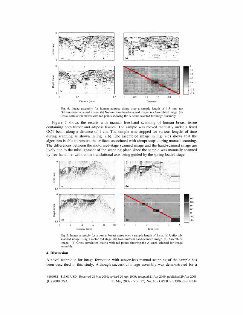
technique for images with relatively low SNR. In Fig. 6, human adipose tissue resting on the

spring loaded guide stage, was manually scanned over a distance of 1.5 mm. A threshold

value of 0.7 was used due to the relatively slow rate of decorrelation of adipose tissue. A line

scan rate of 5 kHz was used for A-scan acquisitions. The assembled image in Fig. 6(c) has

good correlation with the galvanometer scanned image in Fig. 6(a). Limitations in the

algorithm are apparent at the lateral displacement of 0.3-0.5 mm in Fig. 6(c) which are

believed to be due to hand vibrations while trying to hold the spring-loaded stage still. These

vibrations cause rapid decorrelation of the A-scans which the algorithm misinterprets as valid

probe displacements.



Dep

th (

mm

)D

epth

(m

m)

0

1

0

1

(a) (b)

(c) (d)

(a) (b)

(c)

0 0.5 1 1.5 0 0.2 0.4 0.6 0.8 1

1

0.8

0.6

0.4

0.2

0

-0.2

-0.4

Fig. 6. Image assembly for human adipose tissue over a sample length of 1.5 mm. (a)

Galvanometer-scanned image. (b) Non-uniform hand-scanned image. (c) Assembled image. (d)

Cross-correlation matrix with red points showing the A-scans selected for image assembly.

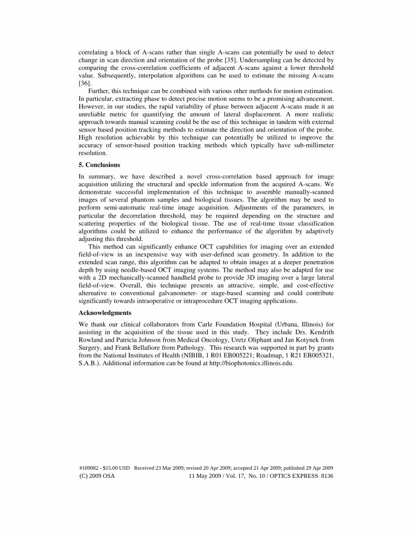
Figure 7 shows the results with manual free-hand scanning of human breast tissue

containing both tumor and adipose tissues. The sample was moved manually under a fixed

OCT beam along a distance of 1 cm. The sample was stopped for various lengths of time

during scanning as shown in Fig. 7(b). The assembled image in Fig. 7(c) shows that the

algorithm is able to remove the artifacts associated with abrupt stops during manual scanning.

The differences between the motorized-stage scanned image and the hand-scanned image are

likely due to the misalignment of the scanning plane since the sample was manually scanned

by free-hand, i.e. without the translational axis being guided by the spring loaded stage.

(a) (b)

(c) (d)


Dep

th (

mm

)D

epth

(m

m)

0

1.5

0

1.5

0 2 4 6 8 10 0 1 2 3 4 5

1

0.8

0.6

0.4

0.2

0

-0.2

-0.4

Fig. 7. Image assembly for a human breast tissue over a sample length of 1 cm. (a) Uniformly

scanned image using a motorized stage. (b) Non-uniform hand-scanned image. (c) Assembled

image. (d) Cross-correlation matrix with red points showing the A-scans selected for image

assembly.

4. Discussion

A novel technique for image formation with sensor-less manual scanning of the sample has

been described in this study. Although successful image assembly was demonstrated for a


range of phantom samples and biological tissues, there are certain limitations that need to be

accounted for when performing real-time in vivo imaging. In this section, we present a

discussion on applicability, limitations, and scope of further improvements in this image

assembly technique.

In order to ensure image assembly while minimizing distortions and inaccuracies, the

decorrelation curves need to be carefully calibrated with the lateral displacement. Selecting

the right threshold is important for accurate image assembly. The current selection method

was based on the decorrelation curves of the particular sample. Plots similar to those shown in

Fig. 3(a) were used to select the optimal threshold for displacement separation. This technique

will work best in highly scattering tissues where decorrelation lengths, governed by the

speckle size, are given by the lateral resolution of the system. The results show that there exist

inter-sample and intra-sample variations in the correlation coefficients at each lateral

displacement. These variations can be attributed to inhomogeneity of structural features in

tissues, variability in speckle patterns, and noise in the system.

However, the results can be significantly improved by adaptively modifying the threshold

value to make the decorrelation curves less sensitive to the changing image features. This

suggests that it would be beneficial to utilize real-time tissue classification algorithms to

adaptively adjust the threshold value [33]. Further experiments also need to be done to

investigate the dependency of various parameters on the decorrelation curves. It is also to

be noted that the decorrelation curves decay down to a small cross-correlation coefficient

value beyond the transverse resolution of the system. A lower threshold based on this value

can provide accurately spaced images, but at the expense of a lower sampling factor and

associated degradation in image quality.

This technique may impose certain limitations on the speed of image acquisition. Our

experimental results show that a sampling factor as high as ~ 50 may be necessary for good

results. Hence the velocity of the probe has to be constrained so that the sample is sufficiently

oversampled. However, this limitation could be easily countered due to the availability of

high-speed OCT systems [4, 34]. While commercial OCT systems have scan rates in the range

of 25-40 kHz, fast swept-source or spectrometer-based OCT systems can extend the A-scan

rates to several hundreds of kHz. For instance, a typical Fourier-domain OCT system with a

25 kHz A-scan rate may allow a probe with 16 µm lateral resolution to be moved with a

maximum velocity of 8 mm/s while still allowing a sampling factor of 50. Hence fast OCT

systems would allow reasonable freedom to allow free-hand manual scanning without

compromising the effectiveness of the algorithm. An attractive feature of this technique is the

relative computational and numerical simplicity which can enable image acquisition to be

done in real-time.

Changes in scanning direction or variation in the angular orientation of the beam will

cause misrepresentation of the images in the current algorithm, when compared to the

galvanometer-based scanning that occurs in a single well-defined two-dimensional plane. The

present algorithm only attempts to assemble images of samples moved in a lateral plane, but

by selecting depth-dependent regions along each A-scan from which to do cross-correlations

between adjacent A-scan regions, it may be possible to track angular out-of-plane

displacements as well. The intended application for this approach is to assemble large images

over scan ranges that exceed the capabilities of current galvanometers and computer-

controlled scanning techniques. In cases for a hand-held probe, needle-probe, or catheter, the

precise in-plane orientation of the acquired data may not be as critical as it is to capture

adjacent A-scans over large lateral distances. Motion artifacts due to hand vibrations or jitter

are more difficult to compensate because the technique is not sensitive to direction of

displacement between A-scans. In our experiments these artifacts arise due to slight jitter of

the hand while trying to hold the manually movable spring-loaded translational stage still. In

the cross-correlation matrix these artifacts appear as varying coefficients with relatively low

value. More sophisticated algorithms can be designed to compensate for these effects. Cross-


correlating a block of A-scans rather than single A-scans can potentially be used to detect

change in scan direction and orientation of the probe [35]. Undersampling can be detected by

comparing the cross-correlation coefficients of adjacent A-scans against a lower threshold

value. Subsequently, interpolation algorithms can be used to estimate the missing A-scans

[36].

Further, this technique can be combined with various other methods for motion estimation.

In particular, extracting phase to detect precise motion seems to be a promising advancement.

However, in our studies, the rapid variability of phase between adjacent A-scans made it an

unreliable metric for quantifying the amount of lateral displacement. A more realistic

approach towards manual scanning could be the use of this technique in tandem with external

sensor based position tracking methods to estimate the direction and orientation of the probe.

High resolution achievable by this technique can potentially be utilized to improve the

accuracy of sensor-based position tracking methods which typically have sub-millimeter

resolution.

5. Conclusions

In summary, we have described a novel cross-correlation based approach for image

acquisition utilizing the structural and speckle information from the acquired A-scans. We

demonstrate successful implementation of this technique to assemble manually-scanned

images of several phantom samples and biological tissues. The algorithm may be used to

perform semi-automatic real-time image acquisition. Adjustments of the parameters, in

particular the decorrelation threshold, may be required depending on the structure and

scattering properties of the biological tissue. The use of real-time tissue classification

algorithms could be utilized to enhance the performance of the algorithm by adaptively

adjusting this threshold.

This method can significantly enhance OCT capabilities for imaging over an extended

field-of-view in an inexpensive way with user-defined scan geometry. In addition to the

extended scan range, this algorithm can be adapted to obtain images at a deeper penetration

depth by using needle-based OCT imaging systems. The method may also be adapted for use

with a 2D mechanically-scanned handheld probe to provide 3D imaging over a large lateral

field-of-view. Overall, this technique presents an attractive, simple, and cost-effective

alternative to conventional galvanometer- or stage-based scanning and could contribute

significantly towards intraoperative or intraprocedure OCT imaging applications.

Acknowledgments

We thank our clinical collaborators from Carle Foundation Hospital (Urbana, Illinois) for

assisting in the acquisition of the tissue used in this study. They include Drs. Kendrith

Rowland and Patricia Johnson from Medical Oncology, Uretz Oliphant and Jan Kotynek from

Surgery, and Frank Bellafiore from Pathology. This research was supported in part by grants

from the National Institutes of Health (NIBIB, 1 R01 EB005221; Roadmap, 1 R21 EB005321,

S.A.B.). Additional information can be found at http://biophotonics.illinois.edu.


Cross-correlation-based image acquisition...

Documents

Transcript of Cross-correlation-based image acquisition...