Critical Density Thresholds in Distributed Wireless Networks

Bhaskar Krishnamachari, Stephen B. Wicker, Ramon Bejar, Marc PearlmanCornell University, Ithaca, NY 14853

{bhaskar@ece,wicker@ece,bejar@cs,pearlman@ece}.cornell.edu

Abstract

We present experimental and analytical results showing “zero-one” phase transitions for network connec-

tivity, multi-path reliability, neighbor count, Hamiltonian cycle formation, multiple-clique formation, and

probabilistic flooding. These transitions are characterized by critical density thresholds such that a global

property exists with negligible probability on one side of the threshold, and exists with high probability on

the other. We discuss the connections between these phase transitions and some known results on random

graphs, and indicate their significance for the design of resource-efficient wireless networks.

1 Introduction

Distributed, multi-hop wireless networks, also known as ad-hoc networks, are gaining in importance as a

subject of research [18], [23]. Their expected applications range from static environmental sensing to mobile

networking for disaster recovery. Many of these applications are likely to involve large-scale operation with

hundreds or thousands of wireless communication nodes.

In large-scale complex systems consisting of many component “particles,” global effects can emerge abruptly

at a critical level of interactions between these components [9]. In physical systems, for example, there are

phase transitions in macroscopic properties such as ferromagnetism or superconductivity that occur abruptly

at a threshold temperature (which regulates the level of interactions between particles). We show here that

analogous critical transitions occur for various properties in distributed wireless networks. A simple example

is that of network connectivity, which we discuss in greater detail in section 2. There exists a critical level

of radio transmission power for all nodes beyond which the multi-hop network formed by n nodes randomly

located in an area is likely to be connected with high probability (nearly one) and below this critical level the

network is likely to be connected with low probability (nearly zero). This has implications for energy-efficient

network design, as the most efficient operating point for the system is just to the right of this transition.

1

An excellent, unifying, tool to help us understand these kinds of effects is the mathematical theory of random

graphs [3]. We review the rudiments of this theory in section 3, and make the connection to our domain

by describing random graph models that are applicable to distributed wireless networks in section 4. Using

these models, we illustrate the existence of phase transitions in a number of other useful properties in wireless

networks in section 5. These properties include multi-path connectivity, Hamiltonian cycle formation, and

connectivity under probabilistic flooding. While random graphs with independence properties have been

widely studied by mathematicians since the 1960’s, exact analytical results are a little harder to obtain for

the random graph models that are useful for distributed wireless networks. On the other hand, obtaining

bounds on the critical density thresholds is somewhat easier. We illustrate this approach with simple but

useful bounds in section 6. Knowing (or at least bounding) the value of the critical density threshold is

useful for design. We conclude in section 7 by discussing the importance of studying these transitions and

the corresponding density thresholds.

2 Connectivity in multi-hop wireless networks

Gupta and Kumar [8] have shown that if we assume each node in an ad-hoc network has constant power,

there is a critical transmission power required to ensure with high probability that two nodes in the network

can communicate with each other through multi-hop paths. There is, in fact, a “phase transition” that

takes place around this critical transmission power level. It is desirable to minimize the energy consumption

of the wireless nodes, but if the node transmission powers are decreased below the critical level, there is a

precipitous drop in the probability that the network is connected.

Specifically, Gupta and Kumar show that if n nodes are placed uniformly and independently in a disc of

unit area in R2, and each node transmits at a power level so as to cover an area of πR2 = (log n + c(n))/n,

then the network is connected with probability asymptotically tending to one if and only if c(n) →∞.

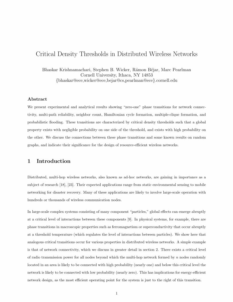
This behavior can be seen in figure 1 which depicts simulated results of multi-hop networks. The plot on

the left shows curves for the probability that n nodes randomly located in a unit square form a connected

network, as the communication radius R is increased. The figure on the right shows the three regions for

one of these curves (n = 100). Region A is undesirable - if transmission powers of the nodes fall in this range

then the network is almost certainly going to be disconnected. Region C is desirable - here the network is

guaranteed to be connected with high probability. From a power-conservation perspective, the point just to

the right of the phase transition region B is the ideal operating point for the system.

2

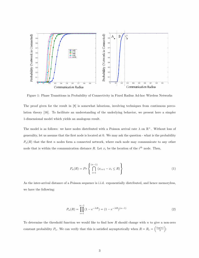
Figure 1: Phase Transitions in Probability of Connectivity in Fixed Radius Ad-hoc Wireless Networks

The proof given for the result in [8] is somewhat laborious, involving techniques from continuous perco-

lation theory [16]. To facilitate an understanding of the underlying behavior, we present here a simpler

1-dimensional model which yields an analogous result.

The model is as follows: we have nodes distributed with a Poisson arrival rate λ on R+. Without loss of

generality, let us assume that the first node is located at 0. We may ask the question - what is the probability

Pn(R) that the first n nodes form a connected network, where each node may communicate to any other

node that is within the communication distance R. Let xi be the location of the ith node. Then,

Pn(R) = Pr

(n−1)⋂i=1

(xi+1 − xi ≤ R)

(1)

As the inter-arrival distance of a Poisson sequence is i.i.d. exponentially distributed, and hence memoryless,

we have the following:

Pn(R) =n−1∏i=1

(1− e−λR) = (1− e−λR)(n−1) (2)

To determine the threshold function we would like to find how R should change with n to give a non-zero

constant probability Pn. We can verify that this is satisfied asymptotically when R = Rc =(

log(n)λ

):

3

Pn

(log(n)

λ

)= (1− e−log(n))n−1 =

(1− 1

n

)(n−1)

(3)

⇒ limn→∞

Pn

(log(n)

λ

)= lim

n→∞

(1− 1

n

)(n−1)

= e−1 (4)

Note that the condition λRc = log(n) is a condition in which each node has log(n) “neighbors” to its right,

hence 2log(n) neighbors on average, analogous to the condition for the threshold function derived for the

2-dimensional case in [8]. The curves obtained by plotting equation (2) with respect to R for a fixed n also

shows the characteristic phase transition behavior seen in figure 1, becoming sharper with n1.

Sanchez et al. showed in [19] that this behavior is in fact robust with respect to different mobility models.

In other words, even when the nodes are moving around, there is still a critical transmission range that is

required to ensure connectivity in the network.

3 Theory of Random Graphs

Such phase-transition behavior has been known to mathematicians for several decades in the form of “zero-

one” laws in Bernoulli Random Graphs [3], [21]. The basic idea is that for certain monotone graph properties

such as connectivity, as we vary the average density of the graph, the probability that a randomly generated

graph exhibits this property asymptotically transitions sharply from zero to one at some critical threshold

value.

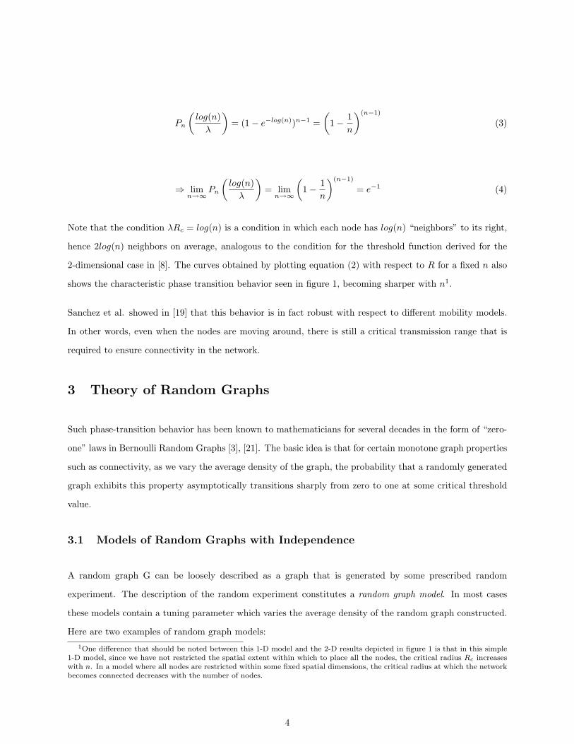
3.1 Models of Random Graphs with Independence

A random graph G can be loosely described as a graph that is generated by some prescribed random

experiment. The description of the random experiment constitutes a random graph model. In most cases

these models contain a tuning parameter which varies the average density of the random graph constructed.

Here are two examples of random graph models:1One difference that should be noted between this 1-D model and the 2-D results depicted in figure 1 is that in this simple

1-D model, since we have not restricted the spatial extent within which to place all the nodes, the critical radius Rc increaseswith n. In a model where all nodes are restricted within some fixed spatial dimensions, the critical radius at which the networkbecomes connected decreases with the number of nodes.

4

Figure 2: Bernoulli Random Graphs

1. Fixed edge number model: G = G(n, e), given e and n, choose G randomly from all graphs consisting

of n vertices and e edges.

2. Bernoulli model: G = G(n, p), given n, and p, construct G with n vertices such that there is an edge

between any two pairs of nodes with probability p. When p = 0, the resulting random graph has no

edges, while when p = 1, we always get the complete graph Kn. As the parameter p increases from 0

to 1, the average density of the random graphs increases (see figure 2).

3. Dynamic model: G = G(n, t), given n and a positive integer t, at each time step t add an edge uniformly

at random (from the possible additional edges) to a graph with n vertices. Hence there are t edges at

time step t.

There is considerable literature on the properties of these random graph models [3]. These models are

somewhat tractable to analysis because they show strong independence properties. In the Bernoulli model,

for example, the probabilities of any two different edges being part of a generated graph are independent of

each other.

3.2 Phase Transitions in Random Graphs

To quote Bollobas : “one of the main aims of the theory of random graphs is to determine when a given

[graph] property is likely to appear... Erdos and Renyi were the first to show that most monotone properties

appear rather suddenly. In rather vague terms, a threshold function is a critical time, before which the

property is unlikely and after which it is likely” [3].

5

Figure 3: Fixed Radius Random Graphs

Let us consider one example of a zero-one law for Random Graphs which applies for first order graph

properties [21]. First order properties of graphs are those that can be described using a language consisting of

the basic Boolean logic connectives (∧,∨,¬), existential and universal quantifiers (∃,∀), variables depicting

nodes, equality and adjacency (written I(x, y)). Examples of first order properties are a) “there are no

isolated points” (∀ x)(∃y)(I(x, y)), and b) “contains a triangle” (∃x, y, z)(I(x, y) ∧ I(x, z) ∧ I(y, z)).

Theorem 1 For every first order graph property A, limn→∞

Pr[G(n, p) has A] = 0 or 1.

Further, if A is a monotone property, then Pr[G(n, p) has A] is also monotone. Thus asymptotically, for

large n, the probability of a random graph property undergoes a sharp zero-one transition for some critical

edge parameter value p = pcrit.

We believe that there is a strong relationship between properties which satisfy a zero-one law for Bernoulli

Random Graphs and properties that also satisfy a zero-one law for random graph models of multi-hop

wireless networks.

4 Random Graphs in Wireless Networks

We now describe two models of random graphs that are useful in studying multi-hop wireless networks - the

fixed radius model and the dynamic probabilistic flooding model.

1. Fixed radius model: Consider an ad-hoc wireless network with n nodes, located randomly in a square

area of unit size, each of which is assumed to transmit with a fixed radio power in an idealized

6

environment where it can be heard by other nodes that are within some radius r. Thus two nodes

can communicate directly with each other if and only if they are no more than a distance r apart.

We can now talk about the underlying communication graph G∗ = G∗(n, R) in this fixed radius (FR)

model - at a given instant let each node in the network correspond to a unique vertex in G∗, with an

edge between a pair of vertices if the corresponding nodes can communicate with each other. Figure

3 illustrates sample random graphs generated according to this model. As the parameter R increases

from 0 to√

2, the average density of the random graphs increases.

2. Dynamic Probabilistic Flooding model: G = G(H, s, q, t), given a communication graph H, a source

node s in H, a probability of forwarding q, and time steps t. Let Gt−1 be the graph before addition

of edges at time step t. G0 consists only of the node s and no edges. At time step t, for each node in

Gt−1 add all outgoing edges of H that are not in Gt−1 (also add the nodes on the other end of these

edges) independently with probability q in order to generate Gt = G(H, s, q, t). Figure 4 illustrates the

evolution of a probabilistic flooding random graph over time. At each time step, new nodes and the

associated edges are added to the existing graph.

Figure 4: Dynamic Probabilistic Flooding Random Graphs

It is important to note that a random graph generated using the fixed radius model has some different

characteristics than the Bernoulli random graph. Consider three nodes i, j, and k. In the fixed radius model,

“the event that there are links between i and j and j and k is not independent of the event that there is a

link between i and k ... as the former is true given the latter only if j lies in the intersection of two discs of

radius [R] centered at i and k” [8]. Still, they do have some things in common. In both models, there is a

7

parameter which varies the density of the graphs produced. We will show in later sections examples where

phase transitions with respect to the parameter p observed in the Bernoulli graph model also show up with

respect to the parameter R in the fixed radius model. It may thus be possible to apply some results from

the literature on Bernoulli random graphs to fixed radius random graphs that are of interest to us in the

context of wireless ad-hoc networks.

5 Density-Critical Transitions in Wireless Networks

We now show some experimental results that illustrate the existence of phase transitions and critical density

thresholds for a number of global properties in wireless networks.

5.1 Neighbor Count

We first consider the property “all nodes have at least k neighbors.” This is a global property that is often

useful in a wireless network in the context of node localization – each node can determine its local position

relative to nearby nodes if it can receive signals from sufficiently many neighbors. Similar properties are also

useful to consider in wireless sensor networks that are involved in tracking target nodes [1].

This graph property can be written explicitly, using the first-order language of graphs, as follows: (∀x)

(∃y1, y2, . . . yk)(I(x, y1)∧

I(x, y2) . . .∧

I(x, yk)). Hence, as per the zero-one law given in theorem 1, this

property provably undergoes a zero-one phase-transition on Bernoulli random graphs G(n, p).

We present empirical results to show this phase transition for the fixed-radius random graph model that

is useful for representing wireless networks. Figure 5 shows the probability that this property is satisfied,

for various values of k as the transmission range of all nodes is increased. The figure is based on empirical

simulations involving n = 100 nodes located uniformly at random in a square area of unit size. The

probabilities are determined in a frequentist manner, each point evaluated based on 100 random graphs.

5.2 Multi-Path Connectivity

In section 2, we saw that the property of connectivity (“between any pair of nodes in the network graph there

exists at least one multi-hop path”) undergoes a zero-one phase transition at a critical threshold. The same,

it has been shown for Bernoulli random graph models is true for the more general notion of k−connectivity,

(“between any pair of nodes in the network graph, there exist at least k node-disjoint paths”)[3], [7]. This

8

Figure 5: Phase Transitions for Neighbor Count (n = 100)

generalization is useful for multi-hop wireless networks in ensuring reliable communication through diverse,

multiple paths [17], [22]. Figure 6 shows this phase transition empirically for the case of biconnectivity

(k = 2). The figure is based on experiments involving n = 100 nodes located uniformly at random in a

square area of unit size.

Figure 6: Phase Transition in Biconnectivity (n = 100)

5.3 Partition into cliques

For certain cluster based approaches, it may be necessary to partition the network into cliques [1], [4]. The

property “the network graph can be partitioned into cliques of size k” also shows critical-density phase

transitions. Here we consider the situation when k = 3, and n is a multiple of 3. This property can be

expressed as a first order statement ([11]) and hence satisfies the zero-one law for Bernoulli random graphs

described in theorem 1.

9

The decision problem version of this graph property (“Can graph G be partitioned into triangles?”) is NP-

complete. Although we do not go into this issue in this paper, there is a significant connection between the

phase transition threshold and the average complexity of solving such NP-hard problems. This has been

addressed, in the context of wireless networks, in [13]. Figure 7 empirically shows the phase transition for

this problem when n = 9 nodes are located uniformly at random in a square area of unit size2.

Figure 7: Phase Transition in Probability of Partitioning Network into 3-Cliques (Triangles) (n=9)

5.4 Hamiltonian cycle

Another property that can be of interest in multi-hop wireless networks is the existence of a Hamiltonian

cycle (a tour that visits all nodes exactly once) in the network graph. A Hamiltonian cycle is useful for the

purpose of forming token rings in the network, and as part of distributed algorithms for election or mutual

exclusion [15]. It also has some useful applications in one-to-one broadcasting for wireless networks involving

nodes with directional antennae [20].

This property is known to undergo a phase transition in Bernoulli and the Fixed Edge Number models of

random graphs [3], [7]. Figure 8 shows that it also undergoes a phase transition in wireless networks. This

figure is based on empirical data for networks generated by placing n = 7 nodes uniformly at random in a

square area of unit size.

As with the previous problem, the existence of a Hamiltonian cycle is also an NP-complete decision problem

whose average computational complexity is known to peak in the phase transition region both for Bernoulli

random graphs and for the fixed radius random graphs that model wireless networks [6], [13].

2We note that the transition curve would be much sharper for larger network sizes.

10

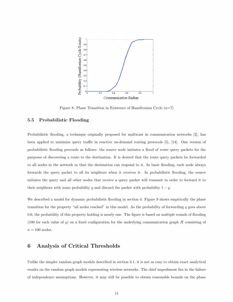
Figure 8: Phase Transition in Existence of Hamiltonian Cycle (n=7)

5.5 Probabilistic Flooding

Probabilistic flooding, a technique originally proposed for multicast in communication networks [2], has

been applied to minimize query traffic in reactive on-demand routing protocols [5], [14]. One version of

probabilistic flooding proceeds as follows: the source node initiates a flood of route query packets for the

purposes of discovering a route to the destination. It is desired that the route query packets be forwarded

to all nodes in the network so that the destination can respond to it. In basic flooding, each node always

forwards the query packet to all its neighbors when it receives it. In probabilistic flooding, the source

initiates the query and all other nodes that receive a query packet will transmit in order to forward it to

their neighbors with some probability q and discard the packet with probability 1− q.

We described a model for dynamic probabilistic flooding in section 4. Figure 9 shows empirically the phase

transition for the property “all nodes reached” in this model. As the probability of forwarding q goes above

0.6, the probability of this property holding is nearly one. The figure is based on multiple rounds of flooding

(100 for each value of q) on a fixed configuration for the underlying communication graph H consisting of

n = 100 nodes.

6 Analysis of Critical Thresholds

Unlike the simpler random graph models described in section 3.1, it is not as easy to obtain exact analytical

results on the random graph models representing wireless networks. The chief impediment lies in the failure

of independence assumptions. However, it may still be possible to obtain reasonable bounds on the phase

11

Figure 9: Phase Transition in Probabilistic Flooding (n=100)

transition. We illustrate this for the neighbor count property we encountered in section 5.1.

We wish to bound the probability that all nodes have at least k neighbors. Let Ai be the event that the ith

node has at least k neighbors. The event that all nodes have at least k neighbors is therefore, {n⋂

i=1

Ai}. The

following shows simple upper and lower bounds on the probability of this event:

1− Pr(Aci ) ≥ Pr(

n⋂i=1

Ai) ≥ 1− nPr(Aci ) (5)

Now it remains to determine what Pr(Aci ) is. Once we fix the location of the ith node, the other n − 1

nodes are located independently, with a uniform distribution, in the square area. If we ignore edge-effects

(by making the boundaries of the unit area overlap), then we wish to determine the probability that less

than k of these n − 1 nodes are located within distance R of the fixed node. Pr(Aci ) is therefore given by

the following expression:

Pr(Aci ) =

k−1∑j=0

(n− 1

j

)(πR2)j(1− πR2)n−1−j (6)

The bounds in expression 5 are illustrated in figure 10 for n = 100 nodes, and k = 2. The lower, union,

bound appears to be quite tight for this situation.

12

Figure 10: Bounds on Probability of all Nodes having 2 Neighbors (n = 100)

7 Discussion and Conclusions

We have shown examples of phase transitions and critical density thresholds for a number of properties in

wireless networks. The connection of this effect to the theory of random graphs suggests that the phenomenon

is quite common.

One cautionary statement is in order: the phase transitions have been illustrated for models with the

assumption that wireless nodes are located with a uniform distribution in an square area. While the shape

of the area is not relevant, the uniformity of the distribution plays a key role. One can easily come up with

situations with highly non-uniform location densities in which the phase transition curves do not provide a

useful measure of whether the network is connected, or if the network satisfies some other global property.

There is evidence to suggest, however, that the phase transition regions are robust to node mobility, provided

that mobility does not break the uniformity of instantaneous location distributions .

Phase transition analysis gives us a tool for analyzing and determining resource-efficient regimes of operation

for wireless networks, with respect to a given global property. For example, if the global property is that

of connectivity, figure 1 tells us that for a uniformly distributed network with a density of 100 nodes per

unit area, the transmission power must be such that the effective communication range is more than 0.25

units (or, equivalently, that each node should have about π ∗ (0.25)2 ∗ 99 ' 20 neighboring nodes, ignoring

edge effects). This density threshold is an energy-efficient point of operation, in that to the left of this

threshold the network is disconnected with high probability, and to the right of this threshold, additional

energy expenditure results in a negligible increase in the high probability of connectivity. The same is true

for the phase transitions and corresponding thresholds illustrated in section 5 for the other properties like

13

k-connectivity, k-neighborhood, Hamiltonian cycle formation, partition into cliques. The phase transition

curve presented for probabilistic flooding also offers the same design lesson; the threshold corresponding

to a high value of the forwarding probability q is a resource-efficient threshold because to the right of this

threshold, redundant messages are sent, wasting precious wireless network resources for negligible gains in

the probability that the flooding succeeds in reaching all nodes in the network.

Of course, it must be kept in mind that increasing the communication range not only makes the network

graph denser, but also increases the level of interference in the network. This increased level of interference

can make it difficult to allocate non-interfering channels to nearby nodes; indeed, the property of conflict-free

channel assignment is known to show a reverse “one-zero” phase transition with respect to interference level

[12]. The intersection of thresholds for such conflicting properties as network connectivity and conflict-free

channel allocation is also important to analyze because this determines the feasible region of operation for

a given wireless network.

We also note that researchers have recently been studying the connection between these kinds of phase transi-

tions and the computational complexity of NP-complete constraint satisfaction problems such as Hamiltonian

cycle and propositional satisfiability [6], [10]. It appears that these results are significant for self-configuration

problems in wireless networks as well. In [13], we have shown that for NP-hard problems in wireless networks

such as the Hamiltonian cycle problem and the problem of partition into cliques, the average computational

complexity (of finding such a cycle or partition) peaks at the phase transition region and decreases consid-

erably as we move to the right of this region.

Thus a study of phase transition phenomena has clear advantages from a design perspective - both for

satisfying desired properties in an energy-efficient manner, and for minimizing the complexity of finding

satisfying solutions. If the analysis is performed off-line before network deployment, it can be used to

predetermine settings for the various node powers, retransmit probabilities etc. A more sophisticated use

of these principles would be the design of distributed, dynamic algorithms that configure themselves to the

resource-efficient edge of the phase transition region.

Other open questions and directions for future work in this area include the quantification of (exact values

or bounds for) density thresholds for various phenomena, the extension of the models to include some level

of non-uniformity in node locations, and explicit consideration of node mobility.

14

References

[1] R. Bejar, B. Krishnamachari, C. Gomes, B. Selman, “Distributed Constraint Satisfaction in a Wireless SensorTracking System,” Workshop on Distributed Constraint Reasoning, International Joint Conference on ArtificialIntelligence, Seattle, Washington, August 2001.

[2] K. Birman et al., “Bimodal Multicast,” ACM Transactions on Computer Systems, Volume 17, No. 2., May 1999.

[3] B. Bollobas, Random Graphs, Academic Press, 1985.

[4] J.C. Cano, and P. Manzoni, “A low power protocol to broadcast real-time data traffic in a clustered ad hocnetwork,” IEEE GlobeCom 2001, November 2001.

[5] R. Chandra, V. Ramasubramanian, and K. P. Birman, “Anonymous Gossip: Improving Multicast Reliability inMobile Ad-Hoc Networks”, International Conference on Distributed Computing Systems, 2001.

[6] P. Cheeseman and B. Kanefsky and W. M. Taylor, “Where the really hard problems are,” IJCAI-91, Vol. 1, pp.331-7, 1991.

[7] J. Frank and C. Martel, “Phase transitions in the properties of random graphs,” Principles and Practice ofConstraint Programming (CP-95), Cassis, France, 1995.

[8] P. Gupta and P. R. Kumar, “Critical Power for Asymptotic Connectivity in Wireless Networks,” in StochasticAnalysis, Control, Optimization and Applications, Eds. W.M.McEneany et al., Birkhauser, Boston, p. 547-566,1998.

[9] S. A. Kauffman, The Origins of Order: Self-organization and Selection in Evolution, Oxford University Press,1993.

[10] S. Kirkpatrick and B. Selman, “Critical behavior in the satisfiability of random Boolean expressions,” ScienceVol. 264, no. 5163, pp. 1297-1301, May 1994.

[11] B. Krishnamachari, S. B. Wicker, and R. Bejar, “Phase Transitions in Wireless Ad-Hoc Networks,” IEEEGlobeCom 2001, November 2001.

[12] B. Krishnamachari, R. Bejar, and S. B. Wicker, ”Distributed Constraint Satisfaction and the Bounds on ResourceAllocation in Wireless Networks,” Sixth International Symposium on Communications Theory and Application(ISCTA ’01), Ambleside, UK, July 2001

[13] B. Krishnamachari, R. Bejar, and S. B. Wicker, “Distributed Problem Solving and the Boundaries of Self-Configuration in Multi-hop Wireless Networks,” 35th Hawaii International Conference on System Sciences, Jan-uary 2002.

[14] L. Li, J. Halpern, Z. J. Haas, “Gossip-based Ad Hoc Routing,” unpublished.

[15] N. A. Lynch, Distributed Algorithms, Morgan Kauffman Publishers, 1996.

[16] R. Meester, and R. Roy, Continuum Percolation, Cambridge University Press, 1996.

[17] M.R. Pearlman, Z.J. Haas, P. Scholander, and S.S. Tabrizi, ”On the Impact of Alternate Path Routing for LoadBalancing in Mobile Ad Hoc Networks,” ACM MobiHOC’2000, Boston, MA, August 11, 2000

[18] C. Perkins (Ed.), Ad Hoc Networking, Addison-Wesley Publishing Co., 2000.

[19] M. Sanchez , P. Manzoni and Z. J. Haas, “Determination of Critical Transmission Range in Ad-Hoc Networks ,”Multiaccess Mobility and Teletraffic for Wireless Communications Workshop (MMT’99), Venice, Italy, October1999.

[20] M. Seddigh and J. S. Gonzales and I. Stojmenovic, “RNG and internal node based broadcasting algorithms forwireless one-to-one networks,” ACM Mobile Computing and Communications Review, Vol. 5, No. 2, pp. 394–397,2001.

[21] J. Spencer, Ten Lectures on the Probabilistic Method, SIAM, 1987.

[22] A.Tsirigos, Z.J. Haas, and S. Tabrizi, ”Multipath Routing in Mobile Ad Hoc Networks or How to Route in thePresence of Topological Changes,” IEEE MILCOM’2001, Tysons Corner,VA, October 28-31, 2001

[23] C. K. Toh, Ad Hoc Mobile Wireless Networks: Protocols and Systems, Prentice Hall, 2001.

15