Critical Density of Spacecraft in Low Earth Orbit: Using ...

LMSEAT-3303

Critical Density of Spacecraft in Low Earth Orbit: Using Fragmentation Data to Evaluate the Stability

of the Orbital Debris Environment

Lockheed Martin Space Operations Company 2400 NASA Rd 1, Houston, TX 77058

February 2000

ii LMSEAT-33303

Critical Density of Spacecraft in Low Earth Orbit: Using Fragmentation Data to Evaluate the Stability

of the Orbital Debris Environment

Prepared by

Donald J. Kessler

Lockheed Martin Space Operations Company

2400 NASA Rd 1, Houston, TX 77058

February 2000

iii LMSEAT-33303

Table of Contents ABSTRACT ...............................................................................................................................1 INTRODUCTION ......................................................................................................................2 BACKGROUND ........................................................................................................................2 P-78 Fragment Data ....................................................................................................................4 P-78 Fragment Data Analysis ......................................................................................................4 Test of Assumptions..................................................................................................................13 Critical Density Redefined ........................................................................................................18 New “Critical Density” Equations .............................................................................................18 Numerical Model ......................................................................................................................20 Contribution of Collision Fragments from all Altitudes.............................................................24 Critical Density under the Assumption of Near-Circular Fragment Orbits .................................30 Critical Number ........................................................................................................................31 Completeness of P-78 Data .......................................................................................................33 Upper-stage Fragmentation Data ...............................................................................................35 Application of Equations and Data ............................................................................................36 Collision Cross-Sections ...........................................................................................................39 Number as a Function of Altitude and Current Regions of Instability ........................................40 Conclusions ..............................................................................................................................45 Acknowledgements...................................................................................................................46 References ................................................................................................................................46 Appendix: Background Equations for Calculating Environment Stability ..................................48

Table of Figures

Figure 1. Spatial Density of P-78 Catalogued Fragments During January, 1986 (234 fragments) ...................................................................................................................6 Figure 2. Spatial Density of P-78 Catalogued Fragments During January, 1987 (189 fragments) ...................................................................................................................7 Figure 3. Spatial Density of P-78 Catalogued Fragments During January, 1988 (137 fragments) ...................................................................................................................7 Figure 4. Spatial Density of P-78 Catalogued Fragments During January, 1989 (57 fragments) .....................................................................................................................8 Figure 5. Spatial Density of P-78 Catalogued Fragments During January, 1990 (18 fragments) .....................................................................................................................8 Figure 6. Spatial Density of P-78 Catalogued Fragments During January, 1991 (16 fragments) .....................................................................................................................9 Figure 7. Spatial Density of P-78 Catalogued Fragments During January, 1992 (11 fragments) .....................................................................................................................9 Figure 8. Spatial Density of P-78 Catalogued Fragments During January, 1993 (9 fragments) .....................................................................................................................10 Figure 9. Spatial Density of P-78 Catalogued Fragments During January, 1994 (9 fragments) .....................................................................................................................10

iv LMSEAT-33303

Figure 10. Spatial Density of P-78 Catalogued Fragments During January, 1995 (9 fragments) .....................................................................................................................11 Figure 11. Spatial Density of P-78 Catalogued Fragments During January, 1996 (9 fragments) .....................................................................................................................11 Figure 12. Spatial Density of P-78 Catalogued Fragments During January, 1997 (8 fragments) ....................................................................................................................12 Figure 13. Spatial Density of P-78 Catalogued Fragments During January, 1998 (8 fragments) ....................................................................................................................12 Figure 14. Spatial Density of Modeled Collision Fragments in Kessler, 1991 (Solar Activity = 110, 300 Fragments Generated) ..............................................................13 Figure 15. Spatial Density of P-78 Catalogued Fragments Larger than 0.68 kg During January, 1986 (68 fragments) ............................................................................................16 Figure 16. Spatial Density of P-78 Catalogued Fragments Larger than 0.68 kg During January, 1987 (66 fragments)............................................................................................16 Figure 17. Spatial Density of P-78 Catalogued Fragments Larger than 0.68 kg During January, 1988 (88 fragments) ............................................................................................17 Figure 18. Spatial Density of P-78 Catalogued Fragments Larger than 0.68 kg During January, 1988 (41 fragments) ............................................................................................17 Figure 19. Numerical Model Prediction of Possible Future Growth in Fragment Population Due to Collisions. (Assumes maintaining current intact population and eliminating explosions.) .......................................................................................................................22 Figure 20. Numerical Model Prediction of Possible Future Growth in Fragment Population Due to Collisions (Assumes maintaining one half current intact population and eliminating explosions.).....................................................................................................22 Figure 21. Numerical Model Prediction of Possible Future Growth in Fragment Population Due to Collisions (Assumes maintaining two times current intact population and eliminating explosions.).....................................................................................................23 Figure 22. Numerical Model Prediction of Possible Future Growth in Fragment Population Due to Collisions (Assumes maintaining two times current intact population and eliminating explosions.).....................................................................................................23 Figure 23. Numerical Model Prediction of Possible Future Growth in Fragment Population Due to Collisions (Assumes maintaining four times current intact population and

eliminating explosions.).....................................................................................................24 Figure 24. Integral of Spatial Density Over time of P-78 Fragments Larger Than 0.68 kg

(September, 1985 to July, 1998) ........................................................................................28 Figure 25. Contributions of Fragments to a Particular Altitude from Collisions at Various

Altitudes............................................................................................................................29 Figure 26. Integral of Spatial Density Over Time, Weighted to a Constant Solar Activity of 130 (September, 1985 to July, 1998; Masses larger than 0.68 kg) ..................................30 Figure 27. Cumulative Number of P-78 Catalogued Fragments as a Function of Mass

(January 1986)...................................................................................................................35 Figure 28. Spatial Density of All Catalogued Objects (February, 1999)....................................38 Figure 29. Spatial Density of Intact Objects (February, 1999 Catalogue)..................................38 Figure 30. Possible Regions of Instability Below 1020 km (February, 1999 Catalogue)............42 Figure 31. Numerical Model Prediction Using Parameters Obtained from Analysis (Assumes

maintaining current intact population and eliminating explosions.) ....................................43

v LMSEAT-33303

Figure 32. “Best Case” Regions of Instability Below 1020 km (February, 1999 Catalogue)......43 Figure 33. Regions of Instability Below 1550 km (February, 1999 Catalogue) .........................44 Figure 34. Numerical Model Prediction Using Parameters Obtained from Analysis (Assumes

maintaining current intact population and eliminating explosions.) ....................................44

List of Tables

Table 1. Summary of 234 P-78 Fragments catalogued by January 1987, Solar Activity During Previous Year, and Effective Time Interval for F10.7=110 and 130...................................15

Table 2. Values for N0τ from P-78 Fragments larger than 0.68 kg at 525 km altitude. Equation 8 integrated from hmin=300 km to hmax. These values are compared to the sum of AvVt = 208 in Table 1. ..................................................................................................................28

Table 3. Ratio of atmospheric density at 525 km altitude to the atmospheric density at h1 for a solar activity of 130, and the value of N0τ at h1 when hmax = 975 km. ................................28

Table 4. Values for N0τ from P-78 Fragments larger than 0.68 kg at 525 km altitude. Equation 12 is used assuming circular orbits (W=1) and an average solar activity of 130 (ρa=3.76x10-13 kg/m3). These values are compared to the values in Table 2. .........................................31

Table 5. Values for N0τ from P-78 Fragments larger than 0.68 kg as a function of h1, assuming hmax = 975 km. Equation 12 is used assuming circular orbits (W=1) and an average solar activity of 130 (ρa=3.76x10-13 kg/m3). These values are compared to the values in

Table 3. .............................................................................................................................31 Table 6. Upper-stage Explosion Data. Data sample similar to the P-78 data sample where area-

to-mass and RCS are used to determine the number of fragments generated larger than 1/1250 of the dry mass of the upper-stage and the average mass-to-area of those

fragments. ........................................................................................................................36

Errata, page 38: Figures 28 and 29 were originally printed in error, labeled with Spatial Density units of “Number/m3”. The correct units are “Number/km3”, and those labels have been corrected accordingly. Page : 17: Figure 17 changed to represent 59 fragments.

1 LMSEAT-33303

Critical Number of Spacecraft in Low Earth Orbit:

Using Satellite Fragmentation Data to Evaluate the Stability Of the Orbital Debris Environment

By

Donald J. Kessler

Orbital Debris and Meteoroid Consultant February, 2000

ABSTRACT Previous studies have concluded that the existing number-density of satellites in low Earth orbit is above a “critical density.” They predict that fragments from random collisions in low Earth orbit will cause the orbital debris population to increase despite efforts to minimize the accumulation of debris. These studies were based on incomplete data and required extrapolations. The largest uncertainty in these conclusions resulted from the uncertainty in the mass, orbit distribution, and decay rate of fragments generated as a result of catastrophic satellite collisions in Earth orbit. New data is now available that significantly reduces these uncertainties. One set of data is the orbital history of fragments from an intentional collision in space, the 1985 USAF anti-satellite test, P-78. The fragments from this test have now been tracked for a sufficiently long time that they can be used with very few modeling assumptions to test the decay rate of collision fragments. Another set of data is the laboratory hypervelocity breakup of a space-qualified payload. This test resulted in a more accurate determination of the mass of the fragments. And finally, NASA has developed databases that describe intact spacecraft (payloads and upper-stages) and tools that have more accurately determined the physical size, area-to-mass ratio, and mass of fragments from on-orbit fragmentations. This data is examined in detail in this paper. The conclusion is reached that although the fragment characteristics were very different from what previous models predicted, the resulting “critical density” levels are not significantly different from previous predictions. The definition of “critical density” is also examined in detail and new critical density equations are derived. These new equations show that if a given level of intact objects is maintained in a particular region of space then the number of fragments massive enough to catastrophically break up another intact object will seek an equilibrium that is a sensitive function of the level of intact objects. If the current fragment environment is below that equilibrium, then the current environment is defined as unstable. If the equilibrium is an infinite amount of fragments, the environment is defined as a runaway environment. The new equations account for all fragments and allow fragments to decay from one region to another, where the old equations did not. The conclusions are reached that the orbital debris environment for much of low Earth orbit is unstable. Some regions may be slightly above the runaway level. A region around 1400 km is probably above a runaway level; however the rate of increase in fragments is very low. Another region around 900 km may be above a runaway level; however data is required on the hypervelocity breakup characteristics of upper-stages to be conclusive. The rate of increase for collision fragments below 1000 km is currently low, but would increase rapidly with increases in the intact population.

2 LMSEAT-33303

INTRODUCTION A zero population growth of satellites in low Earth orbit might be achieved by a combination of limiting future explosions in Earth orbit, and by requiring future payloads and rocket bodies to reenter at the end of their operational life. However, if the number density of satellites is sufficiently high…above a “critical density”… then a zero population growth might not be possible because collisions between existing satellites could produce fragments at a rate faster than they are removed by atmospheric drag. A satellite population just above the critical density would experience a slowly increasing orbital debris environment, perhaps eventually growing to very high levels, despite efforts to minimize on-orbit explosions and orbital lifetimes. Previous studies have attempted to define the level of critical density (Kessler, 1991; Su, 1993; Anselmo, et. al., 1997), and concluded that certain regions of low Earth orbit are already above the critical density. These studies were based on incomplete data. The studies contained assumptions that caused, in some cases, an under-estimation of the level of critical density, and in other cases, an over-estimation of the level. In addition, the term “critical density” was many times misunderstood. Some readers assumed the exceeding of critical density would result in an immediate exponential increase in the environment. This misunderstanding may have resulted from an unclear definition of terms in some of the previous studies. This paper critically reexamines the assumptions and data used in determining previous critical density levels. The assumptions and older data used in previous studies are similar to one another. New data is now available and will be analyzed here. The definition of critical density is examined and new definitions introduced. While the resulting conclusions are not too different from previous conclusions, these conclusions are reached with greater confidence and, hopefully, lead to a better understanding of the consequences of exceeding critical density levels.

BACKGROUND In Kessler (1991), critical spatial density, S, is given by the equation S = 1/(VσN0τ) (1) where V is the average relative velocity which transforms spatial density into flux and has a value of about 7.5 km/sec, and σ is the average collision cross-section area between orbiting objects and has a value of about 10 m2. Details and intermediate equations for the derivation of Equation 1 are given in the Appendix. The values for V and σ were determined from the orbital and physical characteristics of the 1989 catalogued population; they were found to be nearly independent of altitude for altitudes below 1000 km, and believed to contain little uncertainty. Most of the uncertainty in critical density is believed to be within the N0τ terms, which represents the product of an average number of fragments produced per collision and a time-constant for the orbits of these fragments to decay, respectively. Two significant assumptions contribute to the functional form of this equation. First, the assumption is made that low Earth orbit can be divided into independent altitude bands, where collisions outside each altitude band will not affect the population within an altitude band. An altitude band of 100 km was chosen as a compromise between accounting for as many fragments as

3 LMSEAT-33303

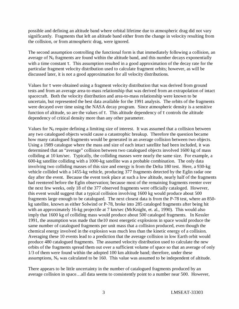
possible and defining an altitude band where orbital lifetime due to atmospheric drag did not vary significantly. Fragments that left an altitude band either from the change in velocity resulting from the collision, or from atmospheric drag, were ignored. The second assumption controlling the functional form is that immediately following a collision, an average of N0 fragments are found within the altitude band, and this number decays exponentially with a time constant τ. This assumption resulted in a good approximation of the decay rate for the particular fragment velocity distribution used to calculate fragment orbits; however, as will be discussed later, it is not a good approximation for all velocity distributions. Values for τ were obtained using a fragment velocity distribution that was derived from ground tests and from an average area-to-mass relationship that was derived from an extrapolation of intact spacecraft. Both the velocity distribution and area-to-mass relationship were known to be uncertain, but represented the best data available for the 1991 analysis. The orbits of the fragments were decayed over time using the NASA decay program. Since atmospheric density is a sensitive function of altitude, so are the values of τ. This altitude dependency of τ controls the altitude dependency of critical density more than any other parameter. Values for N0 require defining a limiting size of interest. It was assumed that a collision between any two catalogued objects would cause a catastrophic breakup. Therefore the question became how many catalogued fragments would be generated in an average collision between two objects. Using a 1989 catalogue where the mass and size of each intact satellite had been included, it was determined that an “average” collision between two catalogued objects involved 1600 kg of mass colliding at 10 km/sec. Typically, the colliding masses were nearly the same size. For example, a 600-kg satellite colliding with a 1000-kg satellite was a probable combination. The only data involving two colliding masses of this size and energy is from the Delta 180 test. Here, a 930-kg vehicle collided with a 1455-kg vehicle, producing 377 fragments detected by the Eglin radar one day after the event. Because the event took place at such a low altitude, nearly half of the fragments had reentered before the Eglin observation; because most of the remaining fragments reenter over the next few weeks, only 18 of the 377 observed fragments were officially cataloged. However, this event would suggest that a typical collision involving 1600 kg would produce about 500 fragments large enough to be catalogued. The next closest data is from the P-78 test, where an 850-kg satellite, known as either Solwind or P-78, broke into 285 cataloged fragments after being hit with an approximately 16-kg projectile at 7 km/sec (McKnight, et. al., 1990). This would also imply that 1600 kg of colliding mass would produce about 500 cataloged fragments. In Kessler 1991, the assumption was made that the10 most energetic explosions in space would produce the same number of catalogued fragments per unit mass that a collision produced, even though the chemical energy involved in the explosion was much less than the kinetic energy of a collision. Averaging these 10 events lead to a prediction that the average collision in low Earth orbit would produce 480 catalogued fragments. The assumed velocity distribution used to calculate the new orbits of the fragments spread them out over a sufficient volume of space so that an average of only 1/3 of them were found within the adopted 100 km altitude band; therefore, under these assumptions, N0 was calculated to be 160. This value was assumed to be independent of altitude. There appears to be little uncertainty in the number of catalogued fragments produced by an average collision in space…all data seems to consistently point to a number near 500. However,

4 LMSEAT-33303

there is considerable uncertainty in the mass of these catalogued fragments, and consequently as to whether all cataloged fragments are capable of causing a catastrophic collision. Consequently, the major uncertainties to be resolved are the mass of collision fragments, how these fragments are distributed in space following a collision, and how the orbits change with time due to atmospheric drag.

P-78 Fragment Data The fragments generated by the P-78 test have produced a unique data set that can be used to help resolve the major uncertainties in determining critical density. This test was conduced September 13, 1985 at an altitude of 525 km…an altitude high enough that most of the fragments that were large enough to be catalogued were catalogued; therefore, the data set is nearly complete. In addition, the test was low enough that most of these fragments have decayed out of orbit, leaving a detailed time history. For example, the early January 1986 catalogue data contains 218 of the 285 total catalogued fragments. An additional 16 objects catalogued within the next year were changing orbital elements so slowly that that their orbits in January1986 could accurately be estimated. Consequently, from January 1986 to the present, we have a detailed decay history of 234 fragments. As of January 1998, only 8 of these fragments were still in orbit. Using the orbital elements in this data set allows calculating the spatial density of collision fragments as a function of altitude at different times. Such a calculation requires no assumptions concerning area-to-mass, or velocity distribution of fragments, and does not require an accurate atmospheric drag model. This procedure allows for a much cleaner, less uncertain, determination of N0τ in Equation 1. The results can be applied to breakups at different altitudes by multiplying the time for the observed orbit changes by the ratio of atmospheric density at the desired altitude to the atmospheric density at 525 km. In the same way, the results can be adjusted to reflect different solar activity conditions. The major assumption is that the P-78 fragments are typical of all collision fragments. This assumption will have to be tested in the future, especially with respect to upper-stages. The applicability of on-orbit upper-stage explosion data will be discussed later. Area-to-mass data and radar cross-section (RCS) data is also available for 202 of the P-78 fragments. The area-to-mass was determined from the decay history of the fragments, as described in the NASA Standard Breakup Model, 1998 Revision (Reynolds, et. al., 1998). A measure of the debris diameter can be determined from the radar cross-section, under the assumption that the ground radar calibration tests, conducted to support the Haystack radar observations using collision fragments generated by ground hypervelocity tests, can be applied to the P-78 fragments (Stansbery, et. al., 1994). Under these assumptions, the mass of 202 of the 234-fragment sample can be calculated.

P-78 Fragment Data Analysis Spatial density as a function of altitude was calculated for each year from January 1986 through January 1998 using the catalogued orbital elements of the P-78 fragments. The same 234 fragments available in 1986 were used for each following year with their new orbit for that year. These results are shown in Figures 1 through 13. Also shown is the number of fragments still in orbit. Compare these figures with the 1991 model predictions for 300 fragments at 500 km, shown in Figure 14,

5 LMSEAT-33303

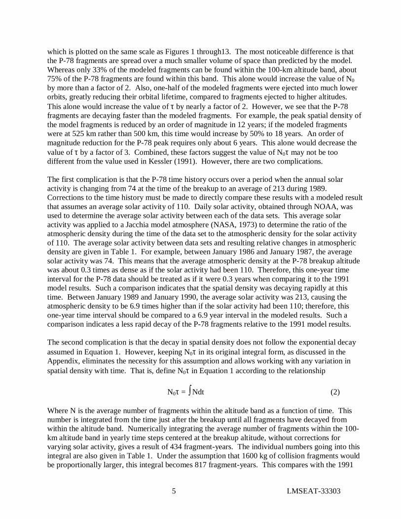
which is plotted on the same scale as Figures 1 through13. The most noticeable difference is that the P-78 fragments are spread over a much smaller volume of space than predicted by the model. Whereas only 33% of the modeled fragments can be found within the 100-km altitude band, about 75% of the P-78 fragments are found within this band. This alone would increase the value of N0

by more than a factor of 2. Also, one-half of the modeled fragments were ejected into much lower orbits, greatly reducing their orbital lifetime, compared to fragments ejected to higher altitudes. This alone would increase the value of τ by nearly a factor of 2. However, we see that the P-78 fragments are decaying faster than the modeled fragments. For example, the peak spatial density of the model fragments is reduced by an order of magnitude in 12 years; if the modeled fragments were at 525 km rather than 500 km, this time would increase by 50% to 18 years. An order of magnitude reduction for the P-78 peak requires only about 6 years. This alone would decrease the value of τ by a factor of 3. Combined, these factors suggest the value of N0τ may not be too different from the value used in Kessler (1991). However, there are two complications. The first complication is that the P-78 time history occurs over a period when the annual solar activity is changing from 74 at the time of the breakup to an average of 213 during 1989. Corrections to the time history must be made to directly compare these results with a modeled result that assumes an average solar activity of 110. Daily solar activity, obtained through NOAA, was used to determine the average solar activity between each of the data sets. This average solar activity was applied to a Jacchia model atmosphere (NASA, 1973) to determine the ratio of the atmospheric density during the time of the data set to the atmospheric density for the solar activity of 110. The average solar activity between data sets and resulting relative changes in atmospheric density are given in Table 1. For example, between January 1986 and January 1987, the average solar activity was 74. This means that the average atmospheric density at the P-78 breakup altitude was about 0.3 times as dense as if the solar activity had been 110. Therefore, this one-year time interval for the P-78 data should be treated as if it were 0.3 years when comparing it to the 1991 model results. Such a comparison indicates that the spatial density was decaying rapidly at this time. Between January 1989 and January 1990, the average solar activity was 213, causing the atmospheric density to be 6.9 times higher than if the solar activity had been 110; therefore, this one-year time interval should be compared to a 6.9 year interval in the modeled results. Such a comparison indicates a less rapid decay of the P-78 fragments relative to the 1991 model results. The second complication is that the decay in spatial density does not follow the exponential decay assumed in Equation 1. However, keeping N0τ in its original integral form, as discussed in the Appendix, eliminates the necessity for this assumption and allows working with any variation in spatial density with time. That is, define N0τ in Equation 1 according to the relationship

N0τ = ∫ Ndt (2) Where N is the average number of fragments within the altitude band as a function of time. This number is integrated from the time just after the breakup until all fragments have decayed from within the altitude band. Numerically integrating the average number of fragments within the 100-km altitude band in yearly time steps centered at the breakup altitude, without corrections for varying solar activity, gives a result of 434 fragment-years. The individual numbers going into this integral are also given in Table 1. Under the assumption that 1600 kg of collision fragments would be proportionally larger, this integral becomes 817 fragment-years. This compares with the 1991

6 LMSEAT-33303

model prediction of 950 fragment-years. That is, with no corrections for atmospheric changes, the P-78 value for N0τ is only slightly less than the 1991 model predictions. Correcting for a solar activity of 110 almost eliminates any disagreement. Such a correction results in a P-78 1600 kg satellite value for N0τ of 952 fragment-years, or almost the same as the 1991 model prediction. This would imply that, under the assumptions used in 1991, critical density should not be changed, and the 1989 environment is above a critical density. However, the P-78 data provides an opportunity to begin testing more of the 1991 assumptions.

SpatialDensity,No./km3

300 400 500 600 700 800 Altitude, km

10-8

10-9

10-10

10-11

Figure 1. Spatial Density of P-78 Catalogued Fragments During January, 1986 (234 fragments)

7 LMSEAT-33303


300 400 500 600 700 800 Altitude, km

10-8

10-9

10-10

10-11



300 400 500 600 700 800 Altitude, km

10-8

10-9

10-10

10-11


8 LMSEAT-33303


300 400 500 600 700 800 Altitude, km

10-8

10-9

10-10

10-11



300 400 500 600 700 800 Altitude, km

10-8

10-9

10-10

10-11


9 LMSEAT-33303


300 400 500 600 700 800 Altitude, km

10-8

10-9

10-10

10-11



300 400 500 600 700 800 Altitude, km

10-8

10-9

10-10

10-11


10 LMSEAT-33303


300 400 500 600 700 800 Altitude, km

10-8

10-9

10-10

10-11



300 400 500 600 700 800 Altitude, km

10-8

10-9

10-10

10-11


11 LMSEAT-33303


300 400 500 600 700 800 Altitude, km

10-8

10-9

10-10

10-11



300 400 500 600 700 800 Altitude, km

10-8

10-9

10-10

10-11


12 LMSEAT-33303


300 400 500 600 700 800 Altitude, km

10-8

10-9

10-10

10-11



300 400 500 600 700 800 Altitude, km

10-8

10-9

10-10

10-11


13 LMSEAT-33303


300 400 500 600 700 800 Altitude, km

10-8

10-9

10-10

10-11

Time interval between curves = 3 years.

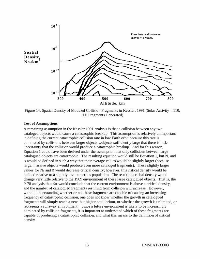
Figure 14. Spatial Density of Modeled Collision Fragments in Kessler, 1991 (Solar Activity = 110,

300 Fragments Generated)

Test of Assumptions A remaining assumption in the Kessler 1991 analysis is that a collision between any two cataloged objects would cause a catastrophic breakup. This assumption is relatively unimportant in defining the current catastrophic collision rate in low Earth orbit because this rate is dominated by collisions between larger objects…objects sufficiently large that there is little uncertainty that the collision would produce a catastrophic breakup. And for this reason, Equation 1 could have been derived under the assumption that only collisions between large catalogued objects are catastrophic. The resulting equation would still be Equation 1, but N0 and σ would be defined in such a way that their average values would be slightly larger (because large, massive objects would produce even more cataloged fragments). These slightly larger values for N0 and σ would decrease critical density; however, this critical density would be defined relative to a slightly less numerous population. The resulting critical density would change very little relative to the 1989 environment of these large catalogued objects. That is, the P-78 analysis thus far would conclude that the current environment is above a critical density, and the number of catalogued fragments resulting from collision will increase. However, without understanding whether or not these fragments are capable of causing an increasing frequency of catastrophic collision, one does not know whether the growth in catalogued fragments will simply reach a new, but higher equilibrium, or whether the growth is unlimited, or represents a runaway environment. Since a future environment is likely to be increasingly dominated by collision fragments, it is important to understand which of these fragments are capable of producing a catastrophic collision, and what this means to the definition of critical density.

14 LMSEAT-33303

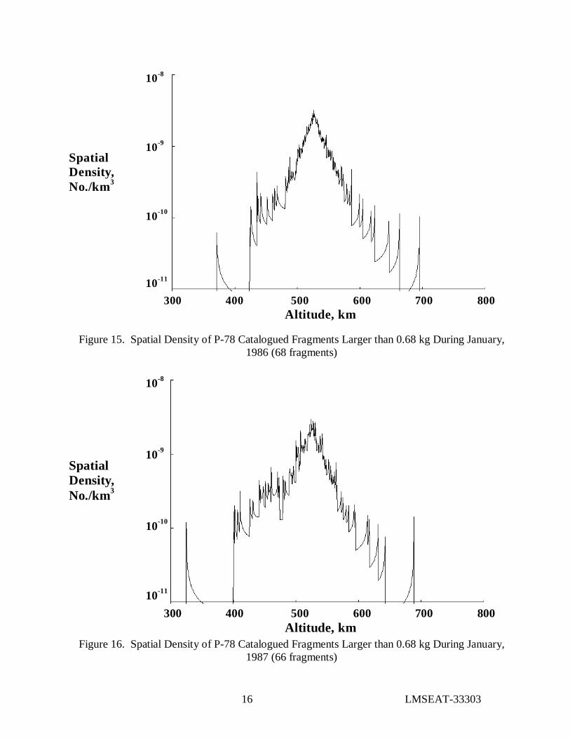
Ground hypervelocity tests have determined that for a collision to be catastrophic at 10 km/sec, the ratio of target mass to projectile mass should be less than 1250 (McKnight, 1992). This would mean that a fragment must have a mass greater than 0.68 kg in order to break up another satellite with the same 850-kg mass as P-78. The area-to-mass and debris diameter data of the P-78 fragments were used to calculate the mass of each of 202 fragments. The sum of these masses was found to be 1179 kg, or larger than the mass of the satellite. This could result from the uncertainty in the calculation of the mass of a single large fragment. However, the assumption will be made that this difference resulted from either an atmospheric density or radar cross-section systematic bias that resulted in the too-large calculated mass of all of the fragments. Therefore, all of the masses were reduced by a factor of 1.5, giving a total fragment mass of 786 kg, leaving 64 kg of fragments not counted. This procedure reduces the 234 fragments in orbit in January 1986 by a factor of more than three to 68 fragments having a mass large enough to catastrophically breakup another satellite the same size as P-78. These 68 fragments were then used to calculate spatial density, as before. The results are given in Table 1 and shown in Figures 15 through 18 for the period January 1986 to January 1989. The figures for January 1990 to January 1998 of fragments larger than 0.68 kg are identical to the corresponding figures for all cataloged objects (Figures 5 -13), because beginning in 1990, only P-78 fragments with a mass greater than 0.68 kg remained in orbit. All fragments with a mass less than 0.68 kg had reentered by January 1990. Comparing Figures 1 through 4 with Figures 15 through 18 illustrate that the more massive fragments were spread over a smaller volume of space. From Table 1, 84% of the fragments in orbit at the end of 1986with mass greater than 0.68 kg are found within the 100 km altitude band, compared to 75% for all fragments. Integrating the number of fragments within the 100-km altitude band, not correcting for atmospheric variation, gives a value for N0τ of 208 fragment-years. This value is just over a factor of 2 less than the value using all fragments, even though the sample of fragments used in the analysis has been reduced by more that a factor of 3. This results from the smaller ejection velocity and longer orbital lifetime of more massive fragments. It means that N0 and τ are not independent variables, and N0 cannot be reduced in number to change the threshold mass without also increasing τ. This emphasizes the need to use the integral in Equation 2 to evaluate N0τ. After correcting to a solar activity of 110, the value of N0τ for fragments larger than 0.68 kg is 365 fragment-years. Little adjustment may be necessary to this value of N0τ to apply it to an average, more massive collision. When the limiting mass of fragments produced in a hypervelocity collision is some fraction of the target (in this case, 1/1250 the target mass), the number of fragments produced may be independent of the target mass. This would be true if the number of fragments varies as the ratio of fragment mass to the target mass, as it does in some satellite and asteroid breakup models. The logic for these types of breakup models is as follows: If the target mass is increased, which would produce more fragments of all sizes, the projectile mass required to cause a catastrophic breakup of the increased target mass must also be increased. The net effect is that the number of fragments produced that are capable of breaking up a satellite of the larger target mass might be the same as for the smaller target mass. There are two other considerations that may increase the value of N0τ. The first consideration is whether all of P-78 fragments larger than 0.68 kg were catalogued; if they were not, then the value of N0 may need to be increased. The second consideration is that larger fragments from a larger satellite might have lower area-to-mass ratios, causing the value of τ to increase. The effect of all

15 LMSEAT-33303

of these considerations is expected to be small; however, they will be discussed in greater detail later. As discussed previously, Earth orbit is currently dominated by collisions between two intact objects, where each collision can be thought of as producing two fragmentation events, possibly doubling the value for N0τ. Therefore, under the assumption that a single breakup produces only 68 fragments that are capable of causing another catastrophic breakup, a value of N0τ somewhere between 365 and 730 fragment-years, but closer to 730, should be used in Equation 1. In addition, as previously discussed, if smaller catalogued fragments are not included, the average size of colliding objects, or the value of σ, must also be increased, all perhaps leading to only a small change in the 1991 critical density prediction. However continuing to use the existing “critical density” equations to refine the 1991 analysis would produce more uncertainty than current data justifies. The P-78 data, better collision breakup models from ground tests, and the area-to-mass ratio data does not justify the assumptions in the 1991 analysis. Although these assumptions can be modified, there is still a need for a better definition of “critical density”, and a better understanding of the consequences of exceeding a critical density, as will be discussed next. Table 1. Summary of 234 P-78 Fragments catalogued by January 1987, Solar Activity During Previous Year, and Effective Time Interval for F10.7=110 and 130

All catalogued fragments Catalogued fragments larger than 0.68 kg Date F10.7 EfT N NVol AvNt EfNt N NVol AvNt EfNt 1986 74 0.30 234 175.0 53 16 68 57 17 5 1987 74 0.30 189 132.5 154 46 66 52 55 16 1988 85 0.48 137 93.0 113 54 59 47 50 24 1989 141 2.1 57 30.9 62 130 41 26 37 77 1990 213 6.9 18 12.8 22 151 18 12.8 19 134 1991 190 5.2 16 8.7 11 56 16 8.7 11 56 1992 208 6.4 11 4.6 7 43 11 4.6 7 43 1993 150 1.6 9 2.5 4 6 9 2.5 4 6 1994 110 1.0 9 2.1 2 2 9 2.1 2 2 1995 86 0.48 9 1.8 2 1 9 1.8 2 1 1996 77 0.34 9 1.4 2 1 9 1.4 2 1 1997 72 0.29 8 1.0 1 0 8 1.0 1 0 1998 80? 0.4? 8 0.8 1 0 8 0.8 1 0 Sum 434 506 208 365 Notes Date: Date of elements set, January of given year. F10.7: Average daily solar activity over previous year (except 1986, where previous 6 months). EfT: Effective time, years. Equal to ratio of atmospheric density due to F10.7 to atmospheric density when F10.7=110 at 525 km. Effective time for F10.7=130 is 0.58 of given values. N: Number of fragments from original sample that were in orbit during January of given year. NVol: Average number of fragments between 475 km and 575 km altitude during January of given year. AvNt: Average number of fragments between 475 km and 575 km during previous year times the number of years fragments are in orbit (1 year for each year except 1986 when fragments were in orbit for 0.3 years. Obtained by averaging number in volume at given year and previous year, then multiplying by 1 year (1987-1998) or 0.3 years (1986). Units are fragment-years. EfNt: Effective fragment-years, due to varying solar activity and is EfT times AvNt. Sum is the effective fragment-years sum if F10.7 had been a constant 110. This sum would be 0.58 the given value if F10.7 had been a constant 130. Note that beginning in January 1990, all remaining fragments had a mass greater than 0.68 kg.

16 LMSEAT-33303


300 400 500 600 700 800 Altitude, km

10-8

10-9

10-10

10-11

Figure 15. Spatial Density of P-78 Catalogued Fragments Larger than 0.68 kg During January,

1986 (68 fragments)


300 400 500 600 700 800 Altitude, km

10-8

10-9

10-10

10-11

Figure 16. Spatial Density of P-78 Catalogued Fragments Larger than 0.68 kg During January,

1987 (66 fragments)

17 LMSEAT-33303


300 400 500 600 700 800 Altitude, km

10-8

10-9

10-10

10-11

Figure 17. Spatial Density of P-78 Catalogued Fragments Larger than 0.68 kg During January, 1988 (59 fragments)


300 400 500 600 700 800 Altitude, km

10-8

10-9

10-10

10-11

Figure 18. Spatial Density of P-78 Catalogued Fragments Larger than 0.68 kg During January, 1988 (41 fragments)

18 LMSEAT-33303

Critical Density Redefined Three improvements in defining critical density are appropriate. The first improvement is to distinguish between a critical density that may best be characterized as an “unstable” environment, and a critical density that is characterized as leading to a “runaway” environment. An “unstable” environment is one that cannot be maintained at its current level because random collisions will cause it to increase. However, the instability would eventually correct itself as the environment increases to a new, higher level and the number of fragments decaying from orbit also increases. A “runaway” environment has no stable level, and would continue to increase as long as the number of intact satellites in orbit is maintained to feed the debris generated by random collisions. The second improvement is to divide the debris population into two groups, intact objects and fragments. This will allow average collision cross-sections to be nearly independent of the limiting size of fragment considered. In addition, as will be seen, it introduces some simplifying concepts that contribute to understanding both unstable and runaway environments. The third improvement is to eliminate the assumption that low Earth orbit can be divided into independent altitude bands, where collisions outside each altitude band will not affect the population within an altitude band. Integrating the contribution from breakups at all altitudes eliminates the need for this assumption. The near-circular orbits of P-78 fragments simplify the understanding of the effects of collision fragments dragging down through lower altitudes. Averaged over a long period of time, the effect of a high altitude breakup on the lower altitudes is the same as if the higher altitude breakup had occurred within the lower altitude band. Consequently, fragments produced at higher altitudes can contribute significantly to instability at lower levels. However, the “altitude band” approach is educational, and can be compared with previous results; consequently, before proceeding with this third improvement, the first two improvements will be developed using the altitude band approach.

New “Critical Density” Equations To develop new definitions for “critical density”, new assumptions are required. The following assumptions seem appropriate, and lead to a simple, consistent set of equations. It will be assumed that the number of intact objects (operational and non-operational payloads, upper-stages, etc.) stays the same within an altitude band. The spatial density of these intact objects is Si and is constant. This is, if an intact object decays from the altitude band or if it breakups up within the altitude band, then another is added; if an object is added, another must be removed. Also within this volume are explosion and collision fragments, each capable of catastrophically breaking up an intact object. These fragments have an initial spatial density of Sf. No new explosion fragments are to be added to the population, and this initial fragment population is allowed to decay. The collision cross-section between two intact objects is σi, and between an intact object and a fragment is σf. A collision between an intact object and a fragment is assumed to generate N0 fragments and a collision between two intact objects generates 2N0 fragments that remain in the altitude band. Each fragment is capable of catastrophically breaking up another intact object. The characteristic decay time for these fragments is τ and found by integrating Equation 2. Under these assumptions, the resulting equilibrium spatial density of collision fragments capable of causing catastrophic collision with intact objects is

19 LMSEAT-33303

SB = Si2 σi V N0 τ/(1-Si σf V N0 τ) (3)

Notice that as SiσfVN0τ approaches 1, SB goes to infinity. Therefore, the critical density corresponding to a runaway environment is given by RSi = 1/(σf V N0 τ) (4) Notice that although this expression is similar to Equation 1, some of the terms are defined differently. The expression applies only to intact objects. It says that the conditions for a runaway are independent of the number of fragments in orbit. The term N0τ is applicable to only fragments large enough to break up an intact satellite. From the P-78 analysis thus far, at 525 km, N0τ = 365 fragment-years when solar activity averages 110. The value of σf is the size of an average intact object, and should be smaller than the average cross-section defined in Equation 1. This places the threshold for a runaway environment above the 1991 published critical density values. The threshold for a runaway environment applies to an environment that is about a factor of 2 lower than the total catalogued environment since it applies only to intact objects. This would place the 1989 environment in Kessler 1991 below the level of a runaway environment. However, a more detailed analysis of the current distribution of intact objects and their collision cross-section is required and will be discussed later. The threshold environment for an “unstable” environment does depend on the current fragment population. The question posed is “given a current fragment population, will it increase due to random collision alone?” This question is answered by setting the current fragment population equal to SB in Equation 3, and solving for the value of Si that produces an equilibrium equal to the current fragment population. The current fragment population can be defined as a factor, k, to be applied to the intact population. That is, let Sf = Si/k = SB. The critical density corresponding to an unstable environment becomes USi = 1/[(σf + k σi)V N0 τ] (5) From the similarity between Equations 4 and 5, the threshold for an unstable environment is always less than the threshold for a runaway environment. The value for σi is larger than the value of σf . If all of the intact objects were the same size and fragments were very small compared to intact objects, the collision cross-sectional area between intact objects would be four times the collision cross-sectional area between intact objects and fragments. However, the area distribution of intact objects would likely place this factor somewhere between two and four. If all catalogued fragments were capable of causing a catastrophic collision, then the value for k would be 1, since the number of catalogued fragments is about the same as the number of intact objects. However, this analysis has concluded that only 29% of the P-78 catalogued fragments immediately after the breakup were this massive. If this were typical of all breakups and no orbital decay had taken place, then the value of k would be slightly less than 4. On the other hand, by the time that the P-78 fragments had decayed to about 25% of the original sample (January 1989), then 72% of the fragments were this massive. If the same orbital decay were representative of all explosions, the value of k would be less than 2. If k = 3 and if σi = 3 σf , then USi = RSi / 10, or the threshold for an unstable environment is a factor of ten lower than the threshold for a runaway environment. These values result in a conclusion that the 1989 environment is unstable by approximately the same amount as published in Figure 4 of Kessler

20 LMSEAT-33303

1991. A later, more detailed analysis will provide more accurate values for σf, σi, k and N0 τ and a comparison of the 1999 intact population to the runaway and unstable thresholds. The conclusion was reached in Kessler 1991, that “certain regions of low Earth orbit are already unstable.” This analysis confirms that conclusion with greater confidence. However the publication assumes that an unstable population would continue to increase until “the population of large objects is sufficiently reduced, either by active removal, or by fragmentation.” The analysis thus far leads to the conclusion that the current population may not yet have reached this runaway threshold; rather, the population will increase until an equilibrium is reached. However, the level of equilibrium, given by Equation 3, is a sensitive function of the intact population characteristics. A numerical program that calculates the number of fragments as a function of time can best illustrate this sensitivity, and the time scales involved.

Numerical Model An existing “two-particle in a box” computer program was modified to use the same assumptions used to derive Equation 3. This program does not explicitly look for any equilibrium or solve for critical density levels. Rather, the program calculates the number of collisions and resulting number of collision fragments generated in a 100-km altitude band as a function of time. An approximation in the model calculates the “average” number of fragments generated per collision based on the expected frequency of intact-intact collisions and intact-fragment collisions. This approximation was required since the number of fragments per collision decreases as the number of fragments increases, since an “average” collision is more frequently an intact-fragment collision. The fragments were assumed to decay exponentially, where the value of the time constant is determined from Equation 2. Therefore, for an average solar activity of 110, from the P-78 data, N0 τ = 365 fragment-years, N0 = 57, and τ = 365/57 = 6.4 years at 525 km. At 950 km with a solar activity of 110, the atmosphere is 77 times less dense than at 525 km, so τ = 6.4 x 77 = 493 years at 950 km. A value of τ = 493 years is used to illustrate the growth of the fragment population as a function of time within the altitude band of 900 km to 1000 km. In Kessler 1991, the number of collisions between the 1989 catalogued objects was found to be 0.05 per year for low Earth orbit. The analysis also found that about half of the collisions (0.025 per year) were within the 900-km to 1000-km altitude band, and that the average collision cross-section between all catalogued objects was 10 m2. In a two-particle in a box model, the following assumptions produce the same collision rate: σi = 27.4 m2, σf = 6.45 m2, the number of intact catalogued objects is 600, and the number of catalogued fragments is 600. If 1/3 of the catalogued fragments (i.e., 200 fragments) are massive enough to cause a catastrophic collision with an intact object, the catastrophic collision rate within this band is 0.02 per year. An intact population within the 100-km altitude band of 600 objects gives a value of Si = 8.8X10-9/km3, or about same as the current population of intact objects at this altitude. A fragment population massive enough to cause catastrophic collisions of 200 give a value of k = 3, as previously estimated. These cross-sections and numbers are then assumed in the two-particles in a box model to illustrate sensitivity and time scales of the 1991 critical density predictions; later analysis will provide more accurate values to be applied to the current environment. A collision between a fragment and an intact object is assumed to produce 57 fragments within the 100-km altitude volume, while a collision between two intact objects produces twice as many fragments. Equations 3, 4 and 5 predict that, under these conditions, the environment would be

21 LMSEAT-33303

unstable, but not a runaway, and would move to an equilibrium of 1576 collision fragments, or a factor of 8 above their initial value. Figure 19 gives the results of the two-particle in a box model under these assumptions. The figure illustrates that over the first 100 years, the amount of increase is very small. The sudden increase every 50 years represents new fragments produced from a collision. After each collision, the fragments decay due to atmospheric drag. After a thousand years, the average number of fragments is beginning to stop increasing, approaching equilibrium. When the results are extended to 4000 years, the program shows that equilibrium is reached at about 1300 fragments, very close to that predicted by Equation 5. The difference between the numerical program equilibrium and the equation 5 prediction is assumed to be due to the approximation in the numerical program describing the average number of fragments produced per collision. In the Figures 20 through 23, only the number of intact objects is changed. In Figure 20, the number of intact objects is reduced to 1/2 its current value, or 300 objects. This number is of interest because it is just over the threshold for instability predicted by Equation 5. Note that over a 1000-year time period, the average number of fragments in orbit remains nearly constant, fluctuating slightly higher than 200 as each collision suddenly increases the environment. Figures 21 and 22 double the current intact population to 1200, and are shown on two different scales. Such an environment might result in about 40 years if operational procedures to limit future orbital lifetimes are not implemented, or within the next 10 years if a major constellation is placed at this altitude. Equations 3, 4 and 5 still predict this environment is unstable but not a runaway environment. According to Equation 5, this environment should reach equilibrium when the fragment population reaches 16,500. Figure 21 illustrates that this 1200-intact-object environment would increase much more rapidly than the 600-intact-object environment, increasing to a level in 150 years that had taken 1000 years in the 600-object environment. Figure 22 expands the figure scale to illustrate that the population is approaching equilibrium. However, the program predicts equilibrium is not reached until about 5000 years, at a level of 10,000 fragments…less than predicted by Equation 5, but still close. Equation 4 predicts a runaway environment when the intact population is 1570 objects. Figure 23 illustrates the results of an intact population of 2400 objects. This figure illustrates an increasing rate of increase for the fragment population, as expected for a runaway environment. Figures 19 through 23 then illustrate the interpretation of Equations 3 through 5. All of these results have assumed an average solar activity of F10.7 = 110. This may be too low a value to represent long term average solar activity…a value closer to 130 may be more appropriate. If so, the value of N0τ, as noted in Table 1,would decrease to 0.58 of its value for a solar activity of 110, so that the value of N0τ at 525 km becomes 212, or about the same as the 208 from the uncorrected data. However, as mentioned earlier, the approach to derive these equations contains an assumption that, if eliminated, could again raise the value of N0τ. The assumption that low Earth orbit can be divided into independent altitude bands ignores the consequences of collisions inside adjacent bands and does not account for all of the fragments. In reality, collision fragments move from one band to another. Therefore, this assumption will now be looked at more closely.

22 LMSEAT-33303

Number of fragments capable of catastrophic collision with an intact object between 900 km and 1000 km altitude

0 200 400 600 800 1000 Time, years

2000

1000

0

Intact population =600initial fragments =200

Figure 19. Numerical Model Prediction of Possible Future Growth in Fragment Population Due to

Collisions. (Assumes maintaining current intact population and eliminating explosions.)


0 200 400 600 800 1000 Time, years

2000

1000

0


Figure 20. Numerical Model Prediction of Possible Future Growth in Fragment Population Due to Collisions (Assumes maintaining one half current intact population and eliminating explosions.)

23 LMSEAT-33303


0 200 400 600 800 1000 Time, years

2000

1000

0


Figure 21. Numerical Model Prediction of Possible Future Growth in Fragment Population Due to Collisions (Assumes maintaining two times current intact population and eliminating explosions.)


0 400 800 1200 1600 2000 Time, years

50000

40000

30000

20000

10000

0


Previous figure

Figure 22. Numerical Model Prediction of Possible Future Growth in Fragment Population Due to Collisions (Assumes maintaining two times current intact population and eliminating explosions.)

24 LMSEAT-33303


0 400 800 1200 1600 2000 Time, years

50000

40000

30000

20000

10000

0


Figure 23. Numerical Model Prediction of Possible Future Growth in Fragment Population Due to Collisions (Assumes maintaining four times current intact population and eliminating explosions.)

Contribution of Collision Fragments from all Altitudes A fundamental function to all of these calculations is the integral of the fragment spatial density over time. Without any corrections for varying solar activity, this integral for P-78 fragments larger than 0.68 kg is very close to the sum of Figures 15 through 18, and Figures 5 through 13. More accurately, it was assumed that Figure 15 represents the altitude profile of fragments from the time of breakup in September 1985 and for the first six months of 1986. Figure 16 is assumed to represent the altitude profile for the last six months of 1986 and the first six months of 1987, and so on. This reduces to the sum of the figures, except for Figure 15, where this figure is weighted by 0.8 years. Figure 24 is the result of that sum. For convenience of discussion this integral is defined as St(h), or

St(h) = ∫Sf dt (6) where h is altitude, and the integral is to be integrated over the time, t, from a time just after the breakup to a time after all fragments have reentered. The peak value of St is at the breakup altitude of 525 km. At higher altitudes, the fragment ejection velocity controls the value of St; at lower altitudes, atmospheric density controls the value. Figure 24 also shows an approximation to St. The approximation below the breakup altitude varies almost exactly inversely as the

25 LMSEAT-33303

atmospheric density varies. Also shown is the 100-km altitude band used to perform all previous analysis. Equation 2 can be rewritten to express N0 as a function of St, or

N0τ = ∫St dU (7) where U is volume. Integrating Equation 7 over the volume interval shown in Figure 24 (from 475 km to 575 km) results in the value for N0τ of 208 fragment-years as given in Table 1. This is the time-averaged number of fragments found within the volume element over their orbital lifetime. However, this average could be obtained by setting up the problem slightly differently. Rather than considering an average breakup to be at 525 km and then sum the contribution over a 100-km altitude band, one could determine the sum of the contributions at an altitude of 525 km from breakups that occur at other altitudes within the volume interval. Two assumptions would be required to cause these approaches to be equal: (1) Breakups are equally likely at all altitudes within the altitude band. (2) The atmospheric density is constant within the altitude band. Figure 25 uses the approximation to St shown in figure 24 to illustrate collision breakups at four different locations under assumptions of a constant atmospheric density and compares this with an actual atmospheric density variation. The top part of Figure 25 illustrates the constant atmosphere assumption. The first panel of Figure 25 illustrates a breakup at 525 km and uses the approximation of St to identify four points and their corresponding spatial density-time values. The value of St at 475 km is A; B is the value at 525 km; C is the value at 575 km; and D is the value at 425 km. Since D is outside of the 100-km altitude band, its contribution is ignored. The number of fragments confined to the 100-km altitude band, as calculated previously by summing their contribution over volume, would be found from A + B + C. To illustrate calculating the contribution to 525 km altitude from breakups at other altitudes, consider the breakup occurring at four locations. When a collision occurs at 525 km, its contribution to 525 km is B, as illustrated in the first panel. The second panel illustrates collision at 475 km; its contribution to 525 km altitude is C. A collision at 575 km, contributes A to 525 km altitude, as illustrated in the third panel. When a collision occurs outside the 100-km altitude band, as in the last panel, its contribution is small, and is ignored. The total contributions from these four examples is B + C + A, or exactly the same contribution as if the three points had been summed in the first panel. With this approach, it is obvious that we need not ignore the contribution from breakups outside the 100-altitude band, even though the contribution may be small. However, as will be seen, the contribution from breakups outside the 100-km altitude band may not be small. The near-circular orbits of the P-78 fragments introduce a simplification that allows eliminating the assumption of a constant atmospheric density. Along the bottom of Figure 25, the above procedure is repeated under the assumption that atmospheric density varies. A, B, C, and D have been replaced with A’, B’, C’ and D’ to represent their corresponding values for breakups at the four different altitudes under the assumption of a varying atmospheric density. A collision at 525 km gives a contribution of B’, which is equal to B, as one would expect. However, a collision at 475 km would produce a value of St that is smaller than C by an amount equal to the

26 LMSEAT-33303

ratio of the atmospheric density at 525 km to the atmospheric density at 475 km. Since St is plotted on a log scale, this ratio is 10-(B-A), and the contribution at 525 km is C’ = C 10-(B-A). Because the slope of the line containing A’ and B’ is the same as the slope that describes the inverse of the atmospheric density, the changing value of St with altitude is simple to illustrate graphically. Graphically, the line containing A’ and B’ is held constant, and line B’C’ is moved along the line containing A’ and B’. The intersection point is B’ and represents the collision altitude. Applying this procedure to determine the contribution A’ from a breakup at 575 km, we find that A’=B. For a breakup at 625 km, the contribution at 525 km is D’, which is also equal to B. In fact, for every breakup above an altitude of 525 km the contribution is B, or the same as if the breakup had occurred at 525 km. The total contribution from these four panels is 3B + C 10-(B-A) and significantly larger than the contribution resulting from assuming a constant atmospheric density. This procedure then illustrates a technique of integrating Equation 7 after removing the assumption that divides low Earth orbit into independent altitude bands. Assume that St(h, h1) is defined as a function of altitude h for a breakup at a particular altitude, h1, and the orbital debris population density is constant between hmin and hmax. The contribution to the integral of Equation 7 from breakups below h1 is the volume integral containing the value of St evaluated at the same distance above h1 as the distance of the breakup altitude below h1, reduced by the ratio of the atmospheric density at h1 and at the breakup altitude. Since the rate of change of atmospheric density with altitude is reflected in the values of St below h1, this function can be used to determine the ratio of atmospheric densities. The contribution to the integral of Equation 7 from breakups above h1 is simply the value of St at h1, times the volume of space between h1 and hmax, or, expressed mathematically,

h1 hmax

N0τ (h1) = ∫ [ St (h) *St (h=2h1-h ) / St (h=h1 )] dU + ∫ St (h=h1) dU (8) hmin h1 where dU is the volume element within altitude dh, or dU = 4π(re+h)2dh and re is the radius of the Earth. If only the second half of Equation 8 is integrated over more than about 50 km altitude, the value of N0τ becomes greater than the value obtained under the previous assumption of an isolated 100-km altitude band. Consequently, several hundred kilometers of altitude contribution can significantly increase the value of N0τ. If the population density of intact objects were constant between hmin and hmax, the equilibrium population of fragments must increase with altitude, as reflected in Equation 3. Therefore, the larger the altitude band the less valid the assumption of a constant orbital debris population. However, as long as the orbital debris population density is increasing with altitude, the value of N0τ (h1) will not be over-estimated and will represent a more accurate value than that obtained using isolated altitude bands. The value for N0τ can now be evaluated under a much less restrictive assumption. Equation 8 will now be used to calculate N0τ(h=525km) under the assumption that breakup rates at altitudes between 525 km and hmax are all equal to or less than the breakup rates at 525 km. The

27 LMSEAT-33303

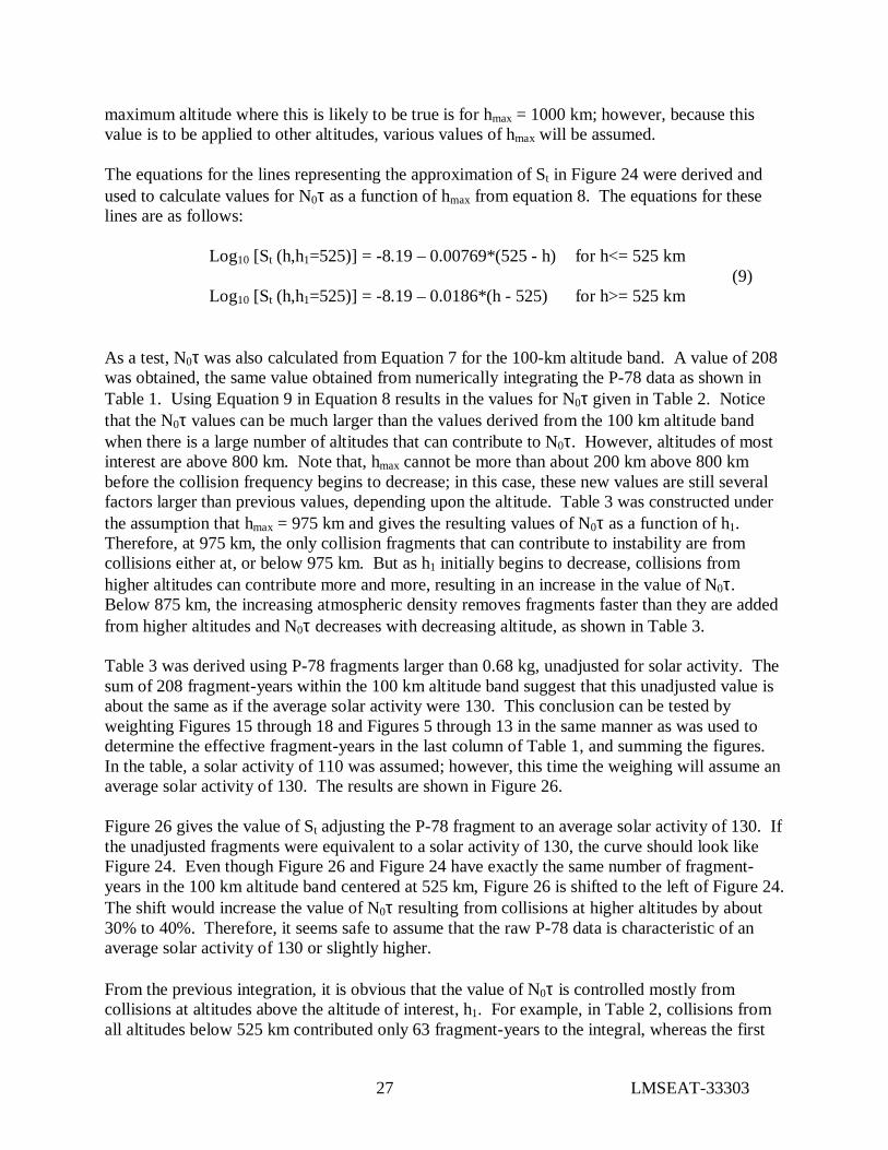
maximum altitude where this is likely to be true is for hmax = 1000 km; however, because this value is to be applied to other altitudes, various values of hmax will be assumed. The equations for the lines representing the approximation of St in Figure 24 were derived and used to calculate values for N0τ as a function of hmax from equation 8. The equations for these lines are as follows: Log10 [St (h,h1=525)] = -8.19 – 0.00769*(525 - h) for h<= 525 km (9)

Log10 [St (h,h1=525)] = -8.19 – 0.0186*(h - 525) for h>= 525 km As a test, N0τ was also calculated from Equation 7 for the 100-km altitude band. A value of 208 was obtained, the same value obtained from numerically integrating the P-78 data as shown in Table 1. Using Equation 9 in Equation 8 results in the values for N0τ given in Table 2. Notice that the N0τ values can be much larger than the values derived from the 100 km altitude band when there is a large number of altitudes that can contribute to N0τ. However, altitudes of most interest are above 800 km. Note that, hmax cannot be more than about 200 km above 800 km before the collision frequency begins to decrease; in this case, these new values are still several factors larger than previous values, depending upon the altitude. Table 3 was constructed under the assumption that hmax = 975 km and gives the resulting values of N0τ as a function of h1. Therefore, at 975 km, the only collision fragments that can contribute to instability are from collisions either at, or below 975 km. But as h1 initially begins to decrease, collisions from higher altitudes can contribute more and more, resulting in an increase in the value of N0τ. Below 875 km, the increasing atmospheric density removes fragments faster than they are added from higher altitudes and N0τ decreases with decreasing altitude, as shown in Table 3. Table 3 was derived using P-78 fragments larger than 0.68 kg, unadjusted for solar activity. The sum of 208 fragment-years within the 100 km altitude band suggest that this unadjusted value is about the same as if the average solar activity were 130. This conclusion can be tested by weighting Figures 15 through 18 and Figures 5 through 13 in the same manner as was used to determine the effective fragment-years in the last column of Table 1, and summing the figures. In the table, a solar activity of 110 was assumed; however, this time the weighing will assume an average solar activity of 130. The results are shown in Figure 26. Figure 26 gives the value of St adjusting the P-78 fragment to an average solar activity of 130. If the unadjusted fragments were equivalent to a solar activity of 130, the curve should look like Figure 24. Even though Figure 26 and Figure 24 have exactly the same number of fragment-years in the 100 km altitude band centered at 525 km, Figure 26 is shifted to the left of Figure 24. The shift would increase the value of N0τ resulting from collisions at higher altitudes by about 30% to 40%. Therefore, it seems safe to assume that the raw P-78 data is characteristic of an average solar activity of 130 or slightly higher. From the previous integration, it is obvious that the value of N0τ is controlled mostly from collisions at altitudes above the altitude of interest, h1. For example, in Table 2, collisions from all altitudes below 525 km contributed only 63 fragment-years to the integral, whereas the first

28 LMSEAT-33303

50 km above 525 km contributed another 195 fragment-years, and for every additional 50 km of altitude another approximately 200 fragment-years are contributed. This results from the fact that the collision fragments are in near circular orbits, and suggest a simplification. Table 2. Values for N0τ from P-78 Fragments larger than 0.68 kg at 525 km altitude. Equation 8 integrated from hmin=300 km to hmax. These values are compared to the sum of AvVt = 208 in Table 1. Max alt, hmax, km: 525 575 625 675 725 775 825 875 925 975 Value of N0τ, frag-yr: 63 258 456 656 859 1065 1274 1486 1701 1919

Table 3. Ratio of atmospheric density at 525 km altitude to the atmospheric density at h1 for a solar activity of 130, and the value of N0τ at h1 when hmax = 975 km.

Altitude h1, km 525 575 625 675 725 775 825 875 925 975 Ratio of atm density: 1.0 2.38 4.55 9.02 16.8 28.8 45.5 66.1 90.2 117 Value of N0τ at h1: 1919 4048 6761 11491 17892 24739 29848 30142 23272 7371

SpatialDensity-time,No.-yr/km3

300 400 500 600 700 800 Altitude, km

10-8

10-9

10-10

10-11

100 km altitude band

Figure 24. Integral of Spatial Density Over time of P-78 Fragments Larger Than 0.68 kg (September, 1985 to July, 1998)

29 LMSEAT-33303

At mospheric densit y varies with altitude and near- circular orbit fragments : Contribution to altit ude h 1 = B’ + C’ + A’ + D’ = 3B +cC.Breakup contribution D’, outside and above the 100 km altitude band, is not s mall but equal to B.

Collision at altitude h1

A

B

C

100 km band

h1

Collision at altitude h1-50 km

B

C

100 km band

h1

Collision at altitude h1+50 km

A

B

100 km band

h1


D

B

100 km band

h1

Collision at altitude h1

A’

B’

C’

100 km band

h1

Collision at altitude h1-50 km

B’

B

C’

100 km band

h1


A’

B’

B

100 km band

h1


D’ B

B

100 km band

h1

Constant at mospheric densit y: Contribution to altit ude h 1 = B + C + A. Breakup contribution D, out side 100 km altit ude band, is s mall, and hasbeen ignored. The heavy li ne is the approxi mation to ∫Sdt in Fi gure 24.

C’=10-( B- A)

C = cc A’ = B D’ = BB’=B

D

Figure 25. Contributions of Fragments to a Particular Altitude from Collisions at Various Altitudes

SpatialDensity-time,No.-yr/km3

300 400 500 600 700 800 Altitude, km

10-8

10-9

10-10

10-11

100 km altitude band

Fit to P-78 data in Fig. 24.Correction to constant solar activity of 130 resulted in a shift of the results to the left, although the average number of fragments found within the 100 km altitude band, centered at the breakup altitude, remained about the same.

30 LMSEAT-33303

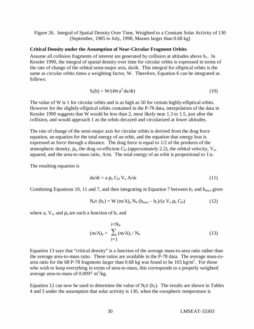
Figure 26. Integral of Spatial Density Over Time, Weighted to a Constant Solar Activity of 130 (September, 1985 to July, 1998; Masses larger than 0.68 kg)

Critical Density under the Assumption of Near-Circular Fragment Orbits Assume all collision fragments of interest are generated by collision at altitudes above h1. In Kessler 1990, the integral of spatial density over time for circular orbits is expressed in terms of the rate of change of the orbital semi-major axis, da/dt. This integral for elliptical orbits is the same as circular orbits times a weighting factor, W. Therefore, Equation 6 can be integrated as follows: St(h) = W/(4π a2 da/dt) (10) The value of W is 1 for circular orbits and is as high as 50 for certain highly-elliptical orbits. However for the slightly-elliptical orbits contained in the P-78 data, interpolation of the data in Kessler 1990 suggests that W would be less than 2, most likely near 1.3 to 1.5, just after the collision, and would approach 1 as the orbits decayed and circularized at lower altitudes. The rate of change of the semi-major axis for circular orbits is derived from the drag force equation, an equation for the total energy of an orbit, and the equation that energy loss is expressed as force through a distance. The drag force is equal to 1/2 of the products of the atmospheric density, ρa, the drag co-efficient CD (approximately 2.2), the orbital velocity, Vo, squared, and the area-to-mass ratio, A/m. The total energy of an orbit is proportional to 1/a. The resulting equation is da/dt = a ρa CD Vo A/m (11) Combining Equations 10, 11 and 7, and then integrating in Equation 7 between h1 and hmax gives N0τ (h1) = W (m/A)a N0 (hmax – h1)/(a Vo ρa CD) (12) where a, Vo, and ρa are each a function of h1 and i=N0

(m/A)a = ∑ (m/A)i / N0 (13) i=1

Equation 13 says that “critical density” is a function of the average mass-to-area ratio rather than the average area-to-mass ratio. These ratios are available in the P-78 data. The average mass-to-area ratio for the 68 P-78 fragments larger than 0.68 kg was found to be 103 kg/m2. For those who wish to keep everything in terms of area-to-mass, this corresponds to a properly weighted average area-to-mass of 0.0097 m2/kg. Equation 12 can now be used to determine the value of N0τ (h1). The results are shown in Tables 4 and 5 under the assumption that solar activity is 130, when the exospheric temperature is

31 LMSEAT-33303

980oK. Comparing these two tables with Tables 2 and 3, respectively, we see that the values of N0τ are about 20% larger in Tables 4 and 5 than the values in Tables 2 and 3. The only exception is, as expected, for the extreme conditions when the maximum hmax-h1 is near zero and no fragments can contribute to h1 under the circular orbit assumption. If the values in Tables 2 and 3 had been calculated after shifting the curves to the left, as suggested by Figure 26, the values in Tables 2 and 3 would be increased by about 35%. If a value of W=1.1 had been used to calculate Tables 4 and 5, the values in Tables 4 and 5 would be 10% higher. These two factors applied to Figures 2, 3, 4, and 5 are justifiable corrections and would cause the values of N0τ obtained under the near-circular orbit assumptions to be in almost-exact agreement with the values of N0τ obtained from the observed changes in the orbits of the P-78 fragments. The common data in these two methods of calculating N0τ is the area-to-mass, which was determined from the decay history of the P-78 fragments. Therefore, the near-circular orbit approach appears to be reasonable. Equation 12 can be combined with Equations 4 and 5, so that RSi (h1) = [a(h1) Vo(h1) ρa(h1) CD] /[σf V(h1) W (m/A)a N0 (hmax – h1)] (14) USi (h1) = [a(h1) Vo(h1) ρa(h1) CD] /[(σf + k σi) V(h1) W (m/A)a N0 (hmax – h1)] (15) Although the two velocities V and Vo have different definitions, their numerical values are about the same and they could cancel out each other. However, when the inclination distribution includes a large number of near polar orbits, such as near 900 km altitude, then the velocity V can be greater than Vo by about 30% (Kessler, 1991). Therefore, these two velocities were left in the new equations. While Equations 14 and 15 look more complicated than Equations 4 and 5, these new equations are expressed in terms of parameters that are much more easily evaluated. Table 4. Values for N0τ from P-78 Fragments larger than 0.68 kg at 525 km altitude. Equation 12 is used assuming circular orbits (W=1) and an average solar activity of 130 (ρa=3.76x10-13 kg/m3). These values are compared to the values in Table 2.

Max alt, hmax, km: 525 575 625 675 725 775 825 875 925 975 Value of N0τ, frag-yr: 0 259 518 776 1035 1294 1553 1811 2070 2329

Table 5. Values for N0τ from P-78 Fragments larger than 0.68 kg as a function of h1, assuming hmax = 975 km. Equation 12 is used assuming circular orbits (W=1) and an average solar activity of 130 (ρa=3.76x10-13 kg/m3). These values are compared to the values in Table 3.

Altitude h1, km: 525 575 625 675 725 775 825 875 925 975 Value of N0τ at h1: 2329 4927 8240 14008 21739 29808 35308 34240 23362 0

Critical Number Multiplying Equations 14 and 15 by the volume of space between h1 and hmax leads to an interesting result, and at the same time illustrates the limitation of assuming near-circular orbits. Such a multiplication converts “critical density” to “critical number”. Equations 14 and 15 become

32 LMSEAT-33303

RNi (h1) = [4πa3(h1) Vo(h1) ρa(h1) CD] /[σf V(h1) W (m/A)a N0] (16)

UNi (h1) = [4πa3(h1) Vo(h1) ρa(h1) CD] /[(σf + k σi) V(h1) W (m/A)a N0] (17) Where RNi (h1) is the number of intact objects maintained above altitude h1 that would lead to a runaway environment, and UNi (h1) is the number for an unstable environment. The interesting result is that neither equation depends upon hmax. This means, for example, no more than 490 intact objects as large as 10 m2 each can be maintained above 1000 km (ρa = 2.96 x 10 –15 kg/m3) without leading to a runaway environment, no matter how large or small the altitude band in which those objects are distributed. The only constraint is the objects are not in independent circular orbits that cannot collide with one another. To illustrate this, assume a constellation of 490 objects that are maintained within a 10-km altitude band just above 1000 km altitude and that these objects are free to randomly collide with one another. The spatial density of these 490 object is Si = 7.2 x 10 –8/ km3. Equation 14 predicts a runaway environment at this spatial density. Now assume that the 490 objects are maintained within a band twice as large, a 20-km altitude band. The spatial density is now reduced by half, but also the runaway threshold from equation 14 is reduced by half. Consequently, whether the constellation is maintained within a 10-km or 20-km altitude band, or even 50-km, maintaining 490 objects in the constellation will lead to a runaway environment. At first, this may seem incorrect. The collision rate between 490 intact objects within a 10-km altitude band is twice the collision rate of these objects within a 20-km altitude band, so one might think it is safer to spread the objects over 20-km. However, in doing so, this provides twice as much time before collision fragments can drag out of the 20-km space. The net effect is that both conditions represent a runaway environment; the only difference is the rate of the runaway. The same prediction can be obtained from Equation 4, where N0τ is obtained from Equation 7, integrating St over a volume of 10 km centered at the breakup altitude. The value of St at 1000 km is obtained from either Figure 24 or 26 by reducing the values of St by the ratio of the atmospheric density at 525 km to the density at 1000 km, or by a factor of 141. Figure 26 predicts a slightly higher runaway density since it reflects fragments remaining near their breakup altitude for shorter times, and spending longer times at lower altitudes. The rate of runaway illustrates an obvious limitation to assuming that fragments are in circular orbits. Suppose the 490 objects were spread between 1000 km and 1050 km. Any fragments produced in a circular orbit at an altitude of 1050 km would require 500 years to drag down to 1000 km altitude and feedback into the collision rate for all 490 objects. However, because collision fragments are actually in slightly elliptical orbits, the fragments are instantly spread out over the 50 km of altitude space following every collision. If the altitude band were even higher, for example between 1000 km and 1500 km, then another issue arises. While the environment may runaway, the coupling between the upper regions of this altitude band and the lower regions of the altitude band is separated by thousands of years. From a practical standpoint, a population a few hundred kilometers above 1000 km is isolated

33 LMSEAT-33303

from events at 1000 km because of the long period of time required for fragments to migrate these few hundred kilometers. Therefore, when considering instabilities in the environment, one might be advised to limit the volume of space to a small enough volume that fragments migrate over that volume, either by collision forces or atmospheric drag, in some reasonable length of time. That reasonable length of time is established by how far we think we can see into the future, by how sure we are of our understanding of the consequences of our actions, and by the level of responsibility we feel about leaving an environment problem for future generations, maybe 100 or 1000 years from now. There is no clear answer. Above 1000 km altitude, it is probably a good idea to consider any regions in low Earth orbit that are separated by more than about 100 km to be independent of one another. At altitudes of tens of thousands of kilometers, collision forces can more easily spread fragments over larger altitude bands, and the regions may have to be separated by more than 100 km to be independent.

Completeness of P-78 Data Until now, it as been assumed that the 68 catalogued fragments larger than 0.68 kg represented a complete sample of fragments of this mass and larger. Figure 27 is a plot of the log of the cumulative number of P-78 fragments as a function of log mass. The plot is close to linear, and follows a collision breakup model where number varies as the ratio of fragment mass to target mass to a power somewhere between –0.75 and –0.85 for sizes larger than 2 kg. This is as expected from most hypervelocity collision breakup models. For sizes smaller than 2 kg, the number does not increase as rapidly, suggesting that some of these fragments may not have been catalogued. Within the size interval between 2 kg and 0.68 kg, there are 31 fragments; 4 of these have diameters derived from their RCS of 15 cm and 2 of these had diameters of only 11 cm. Of all the 234 P-78 fragments, only 2 were determined to have a diameter less than 11 cm; a size of 11 cm is near the absolute smallest size that can be catalogued; sizes as small as 15 cm are difficult to catalogue. The fact that 11 to 15 cm objects were cataloged at sizes larger than 0.68 kg makes it probable that some fragments as small as 0.68 kg had an RCS corresponding to objects smaller than 11 cm. A metal sphere 11 cm in diameter would have to have a mass density of slight less than 1 g/cc to have a mass of 0.68 kg. Consequently, it is possible that a dense metal or even an aluminum fragment could have a physical size of less than 11 cm and a mass greater than 0.68 kg. A linear extrapolation from sizes larger than 2 cm on Figure 27 using a slope between –0.75 and 0.85 suggests that the number of fragments larger than 0.68 kg should be somewhere between 80 and 95. Looking at ground hypervelocity breakup tests leads one to the same conclusion. The only ground hypervelocity breakup test of an actual satellite was the Transit/OSCAR satellite during the SOCIT series of hypervelocity tests. This test, sponsored by the Department of Defense, impacted a 150 g aluminum sphere at 6 km/sec into a 35.4 kg Navy navigation satellite (Hogg, et.al., 1993). The purpose of the test was to characterize in the laboratory the debris generated by a hypervelocity collision in space. The data analysis was completed with funding from NASA to more accurately characterize the resulting fragments. The mass of a fragment which would break up another satellite of Transit mass is 34.5/1250 = 0.0276 kg. The number of loose fragments of this size or larger was about 80. However, the NASA-sponsored analysis concentrated on statistically analyzing the much larger number of fragments that had been captured in foam that lined the chamber. Some of the fragments larger than 0.0276 kg were

34 LMSEAT-33303

captured in the foam. The NASA-sponsored analysis concluded that the number of fragments larger than 0.0276 kg should be about 90 to 100 (McKnight, et. al., 1995), or about the same number of fragments larger than 1/1250 of the target mass suggested from the linear extrapolation of the P-78 data. Consequently, it is reasonable to assume that a catastrophic breakup of a satellite from a hypervelocity collision will produce more than the 68 catalogued fragments of P-78. About 90 fragments is a more realistic number. This would also mean that the approximately 22 fragments that were not cataloged would have small area-to-mass ratios to avoid detection. If these 22 fragments all had a mass of 0.68 kg and an effective diameter of 10 cm, their area-to-mass ratio would be 0.012 sq. m2/kg. Previously, it was determined that the 68 catalogued fragments had an “effective” average area-to-mass ratio of 0.0097 m2/kg; consequently, the uncatalogued fragments would have to be either smaller than 10 cm, or more massive than 0.68 kg, or both to lower this average significantly. Another test to determine whether the effective average area-to-mass should be adjusted is to average the mass-to-area ratios for a larger limiting mass where it can be safely assumed that all of the fragments were catalogued. At a fragment size of 2 kg, the effective average becomes 0.0070 m2/kg; at 3 kg, it becomes 0.0063 m2/kg. The effective average decreases with increasing size. However, such a trend could be explained as simply the result of larger fragments. But, as discussed earlier, an average collision between objects currently in orbit would be slightly larger than the P-78 satellite; consequently, the area-to-mass ratio of these larger fragments may be more representative. Therefore, using an effective average area-to-mass ratio somewhere between 0.0070 m2/kg and 0.0093 m2/kg would be justified based on the P-78 data alone.

Number ofFragmentsof mass mand larger

0.1 1.0 10 100 1000 Mass, kilograms

1000

100

10

0

N ~ m-.8

P-78 Data

35 LMSEAT-33303

Figure 27. Cumulative Number of P-78 Catalogued Fragments as a Function of Mass (January 1986)

Upper-stage Fragmentation Data There is no fragmentation data on the hypervelocity breakup of upper-stages. However, there is data on upper-stage breakups resulting from explosions in orbit. Since nearly half of all intact objects are upper-stages, one should be aware of possible differences in the resulting collision fragment mass and area-to-mass distributions of upper-stages compared to payloads. The on-orbit explosion data may provide some clues. Area-to-mass data on 3,605 explosion fragments from 15 explosions of upper-stages in orbit was derived in the same manner as the area-to-mass data for the P-78 fragments. The diameter of these fragments was determined from the radar-cross section, just as it was with the P-78 fragments. Table 6 is a list of the 15 upper-stage explosions. These 15 events generated a total of 3,741 catalogued fragments and are believed to be representative of some of the more energetic explosions in Earth orbit; consequently, if any explosion can duplicate a hypervelocity collision, these might come closest. Of the 3,605 fragments in the data sample, 1,889 were still in orbit as of July 1999, when there were a total of 3,430 catalogued fragments from all breakups in Earth orbit. Consequently, these 15 explosions represent 55% of the currently catalogued fragment population (Johnson, et. al., 1999). The mass of each fragment was obtained in the same manner as the P-78 fragments, except in this case, the derived mass did not appear to be biased, so no correction factors were applied. The number of fragments with masses larger than 1/1250 of the dry mass of the upper-stage was then obtained and the average mass-to-area of those fragments. These results are also shown in Table 6. Notice that most of the explosions produced a smaller number of the more massive fragments than the 68 fragments produced by P-78. The average number of fragments more massive than 1/1250 of the exploding mass was 49.5 fragments. But even more different than the number was the average mass-to-area ratios. The average mass-to-area ratio of these fragments for P-78 was 103 kg/m2; none of the explosion events produced an average ratio that was greater than half of the P-78 average. The average mass-to-area ratio of all fragments larger than 1/1250 of the upper-stage dry mass was 23.2 kg/m2. These results imply that breakups of upper-stages have significantly less of an effect on the stability of the environment than breakups of payloads, producing fewer fragments massive enough to be of concern and fragments that reenter much quicker than payload fragments. Upper-stages are mostly empty tanks; consequently, one might expect their fragments to be less massive and include the larger area of the sides of the tank. However, there are also a number of reasons to believe that these explosions might not be representative of hypervelocity collisions. The high concentration of energy in a hypervelocity collision can produce more numerous, more dense fragments than an explosion. The low-intensity explosions that caused these breakups are known to produce fewer small fragments (Bess, 1975). The amount of energy that caused these explosions is not known. Even though these explosions produced a larger number of catalogued fragments, most of the fragments were very light and may have resulted from an explosion where little energy was released. Consequently, without verifying tests, this data cannot be considered characteristic of hypervelocity collisions. However, the data suggest important trends that would justify hypervelocity tests.

36 LMSEAT-33303

The explosion data does provide an important measurement to determine the number of fragments currently in Earth orbit that are capable of causing a catastrophic collision. This sample contains 744 fragments larger than 1/1250 of the upper-stage dry mass, or 20% of the number of catalogued fragments produced. These more-massive fragments will likely be the last to decay due to atmospheric drag. Consequently, at altitudes around 1500 km or higher, where few fragments have decayed, the number of the more-massive fragments is slightly more than 20% of the catalogued fragments. Around altitudes of 800 km or lower, the older, lighter fragments may have decayed so that most of the remaining fragments are these more-massive fragments. Table 6. Upper-stage Explosion Data. Data sample similar to the P-78 data sample where area-to-mass and RCS are used to determine the number of fragments generated larger than 1/1250 of the dry mass of the upper-stage and the average mass-to-area of those fragments. Upper-stage, Associated payload

Dry mass, kg

No. Fragments larger than 1/1250 of dry mass

Average mass-to-area kg/m2 of larger fragments

Delta, Landsat 1 800 76 21.2 Delta, Landsat 2 840 57 32.4 Delta, Landsat 3 900 41 23.9 Delta, NOAA 3 840 48 13.7 Delta, NOAA 4 840 32 19.5 Delta, NOAA 5 840 30 18.2 Delta, Nimbus 6 840 40 22.7 Delta, Himawari 900 63 32.1 Agena, Nimbus 4 600 57 15.7 Agena, OPS 7613 600 54 25.2 Titan transtage, OV2 2555 73 46.9 Able Star, Transit 4A 625 91 20.5 Ariane, Spot 1400 25 11.7 SL-16, Cosmos 2227 9000 23 34.0 Long March 4, Feng 1000 34 10.4

Application of Equations and Data Equations have been derived which predict the conditions for an unstable environment, and hypervelocity and explosion data has been analyzed to determine the values of critical parameters in those equations. The equations have been applied to a few hypothetical situations. The equations will now be applied to the current low Earth orbit environment. The low Earth orbit has been described in terms of the catalogued spatial density as a function of altitude, as is shown in Figure 28, using a February 1999 catalogue of 8,631 objects. This catalogue contains orbital information obtained by the US Space Command plus additional information gathered by NASA. The additional information includes a classification of the object type (upper-stage rocket body, payload, operational debris, fragment debris, anomalous debris, and debris distributor), the mass of the object if known, the physical dimensions if known, and an estimated size based on an average radar cross-section using the size-determination model developed to support Haystack radar observations.

37 LMSEAT-33303

Given this data, the first task is to define “intact objects”. Two possibilities were considered: Intact objects could be defined either any object whose mass is known, or as upper-stages and payloads. After some consideration, it was determined that either definition produced about the same results. However the second definition, that intact objects are payloads and rocket bodies, was the most consistent and provided the most flexibility. Some of the objects whose mass was known were the largest fragments of an upper-stage explosion; others were small operational debris with masses that were small and more characteristic of fragments. In addition, this second definition allows looking at payloads and rocket bodies independently, if desired. Figure 29 gives the spatial density of intact objects under the payloads/upper-stage definition. Four regions stand out as regions of high concentration of intact objects: (1) 570 km to 670 km; (2) 750 km to 860 km; (3) 920 km to 1020 km; and (4) 1350 km to 1550 km. Region 2 includes the Iridium constellation that causes the very sharp peak between 775 km and 780 km. The region below 670 km may be sufficiently low that atmospheric drag will remove fragments quickly so that this concentration may not be material; however, it will be included in the analysis since fragments generated in the regions above it will quickly decay into this region. Most fragments generated in region 3 that are massive enough to cause a catastrophic collision will require a few hundred years to decay into region 2, accelerated somewhat by collision scattering. Thus, the long-term stability of region 2 will be assumed to depend on region 3. However, the time for such fragments to decay from region 4 into region 3 is about 8,000 years; consequently, the region above 1350 km will be assumed to have no effect on the regions below 1000 km. Below 1000 km, when payloads and upper-stages are looked at independently, they are found to show the same concentrations as Figure 29, with the spatial density of each being about equal, except in region 4. In region 4, the concentration of intact objects is about 90% payloads and only 10% upper-stages. The difference between Figures 28 and 29 is mostly the spatial density of fragments. This difference for the three regions below 1020 km suggests that the number of catalogued fragments is about equal to the number of intact objects. As discussed earlier, most of the older, catalogued explosion fragments below 800 km are probably massive enough to cause a catastrophic collision with a payload or upper-stage. If it is assumed that half of these fragments are this massive, then the ratio of intact objects to massive fragments, k, is two. That is, an approximate value of k=2 for altitudes below 1000 is consistent with the available data. Near 1500 km the number of catalogued fragments is only about 40% the number of intact objects. Since atmospheric drag has not had a chance to remove many of the high area-to-mass ratio fragments, only about 25% of these fragments are massive enough to cause a catastrophic collision. This leads to a value of k=10 for the region between 1350 km and 1500 km.

38 LMSEAT-33303

Spatial Density, Number/km

3

0 500 1000 1500 2000 Altitude, Km

10 -7

10 -8

10 -9

10 -10

Figure 28. Spatial Density of All Catalogued Objects (February, 1999)

Spatial Density, Number/km

3

0 500 1000 1500 2000 Altitude, Km

10 -7

10 -8

10 -9

10 -10

Figure 29. Spatial Density of Intact Objects (February, 1999 Catalogue)

39 LMSEAT-33303

Collision Cross-Sections Collision cross-sections were determined using the US Space Command/NASA catalogue from both the physical dimensions and the inferred size derived from the RCS. When using the physical dimensions, if the object had only one dimension, it was assumed to be a sphere; if it had a length and one other dimension, it was assumed to be a cylinder, and if it had three dimensions, it was assumed to be a box. When using the RCS-derived size, the object was assumed to be a sphere. The average cross-section was assumed to be 1/4 of the object’s surface area. To determine the average collision cross-section for an intact-fragment collision, it was assumed that a fragment was a point. Therefore, the average collision cross-section of an intact-fragment collision was the average cross-section of intact objects. To determine the average collision cross-section for an intact-intact collision, the same procedure was used as was used in Kessler 1978, where the collision cross-section between any two intact objects was calculated, then summed over the distribution of intact cross-sections for all combinations of intact pairs. For intact objects with an orbital perigee greater than 400 km, and an apogee less than 1100 km, the physical dimensions of the intact objects resulted in the following values: σf = 11.4 m2; σi = 40.5 m2. The ratio of σi /σf = 3.6 is only slightly less than 4, the maximum ratio if all intact objects had been the same size. Using the RCS-derived size resulted in collision cross-sections that were about 65% of those based on physical dimensions. The difference suggests a problem with the size-determination model. This model was derived under the assumption that the radar characteristics of lab-produced fragments was characteristic of all objects in space; this assumption may not be valid for intact objects. Consequently, it will be assumed that the cross-sections derived from the known physical dimensions is characteristic of intact objects. These derived cross-sections appear to be significantly larger than the average of 10 m2 found in Kessler 1991. However, the earlier average cross-section was defined differently and included fragment-fragment collisions. In addition, there is a slight trend toward larger intact objects over the past 10 years. For example, using the 1989 data, a value of σf = 9.7 m2 was obtained based on known physical dimensions at that time. Finally, different assumptions were made if the physical dimensions were not known. In the earlier analysis, if the physical dimensions were not known, the RCS was used, and if the RCS was not available, the size was assumed to be very small. This would tend to bias the results toward smaller sizes. In this analysis, an object is not included in determining average cross-section if no physical information is available. If the exclude objects were “typical”, then no bias should be introduced. Large intact objects at altitudes below 400 km, such as the MIR Space Station, were avoided in determining average collision cross-sections. Between 400 km and 1100 km, these averages are not a sensitive function of altitude, although the regions of highest intact concentrations also include larger intact objects. For Example, the averages for the first region, 570 km to 670 km are σf = 14.4 m2 and σi = 53.8 m2; the second region 750 km to 860 km, σf = 12.0 m2 and σi = 40.3 m2; the third region 920 km to 1020 km, σf = 14.1 m2 and σi = 53.3 m2. The smallest cross-sections are located in the second region. However, this altitude band includes a concentration of near-polar orbits that increases collision rates by a few tens of a percent over those calculated from a more even distribution of orbital inclinations. This increased collision rate could be expressed either in terms of an increased velocity or an increased collision cross-section; it becomes convenient here to express the increased rate in terms of increased collision cross-

40 LMSEAT-33303

section. Consequently, all three regions below 1100 km could be summarized as having σf = 14 m2 and σi = 53 m2. In the fourth region, 1350 km to 1550 km, intact objects are much smaller than those in lower altitudes and the cross-section averages are considerably less. The averages for this region are σf = 2.3 m2 and σi = 6.6 m2. Below 1000 km the average collision cross-sections for payloads only is about 0.35 times the average for intact objects, while the average collision cross-sections for upper-stages is about 1.65 times the average for intact objects. Therefore, even though the number of payloads and upper-stages may be equal, catastrophic collisions involving upper-stages are much more probable than collisions involving payloads. This places increased importance on obtaining data on the hypervelocity breakup of upper-stage rocket bodies.

Number as a Function of Altitude and Current Regions of Instability The current regions of potential instability will now be examined using the derived equations and the values of parameters that go into those equations. Equations 16 and 17 are the form of the instability equations most applicable for the distribution of intact objects in Figure 29. To use these equations, it is assumed that only intact objects below 1020 km contribute to any instability below 1020 km. That is, the region between 1350 km and 1550 km will be considered independent of lower altitudes because of the long period of time for fragments to decay into the lower regions. In Equations 16 and 17 for the regions below 1020 km, the following values represent the most realistic values based on hypervelocity impact data and the current catalogue of objects in orbit: N0 = 90, (m/A)a = 125 kg/m2, σf = 14 m2, σi = 53 m2, W=1.1, CD =2.2, and k=2. Between 1350 km and 1550 km, where average intact sizes are smaller and fewer fragments are found, the following changes are necessary: (m/A)a = 100 kg/m2, σf = 2.3 m2, σi = 6.6 m2, and k=10. At all altitudes, atmospheric densities were determined from NASA SP-8021 under the assumption of an average solar activity of 130. When combined with geomagnetic activity, this solar activity represents an exospheric temperature of 980 degrees Kelvin. Figure 30 gives the number of intact objects found between the given altitude and an altitude of 1020 km. This figure was derived from Figure 29 by multiplying spatial density by volume to obtain number, then summed between 1020 km and the given lower altitude. The figure illustrates that there are just over 1000 intact objects below 1020 km, and about 400 intact objects between 900 km and 1020 km. Also shown are the threshold numbers for both a runaway environment and for an unstable environment from Equations 16 and 17. Where the number of intact objects exceeds these thresholds, maintaining this environment of intact objects will cause the fragment population to increase. If the number of intact objects exceeds the unstable threshold, the increase will be either to a higher but eventually stable value; if the number of intact objects exceeds the runaway threshold, the environment will runaway over an infinite amount of time to an infinite number of fragments. The region of space between 600 km and 1000 km is well above the unstable threshold and the region of space between 800 km and 970 km is above the runaway threshold.

41 LMSEAT-33303

It is instructive to compare the runaway environment for the region near 900 km with the numerical model results illustrated in Figure 19, where an unstable, but not runaway, environment containing 600 intact objects was illustrated for this region. This illustration used a “particle-in-a-box” logic, as did Kessler 1991, which is now shown to place the thresholds for instability at too high a level. The concept that collision fragments “drag through” regions of concern, rather than being scattered by collision forces with some fragments “lost”, lowers the levels of instability. This “drag through” concept, which accounts for all fragments, combined with the realization that not all P-78 fragments larger than 0.68 kg were catalogued, increases the value of N0 to 90, and decreases the thresholds by a factor of 1.6. The concept also allows for the atmospheric density to vary with altitude so that the “average” amount of time that fragments spend within any region is increased. In this case, combined with a slightly higher mass-to-area ratio of fragments not catalogued, the effective value for τ is increased to 729 years, despite the fact that solar activity was increased to 130, lowering the thresholds by another factor of 1.5. However, the largest factor resulted from the increase in the collision cross-section, lowering the thresholds by another factor of 2.2. To illustrate this possible runaway environment, these new values for N0 and τ, as well as the new collision cross-sections, were used in the numerical model to predict a possibly more realistic future environment for this altitude than Figure 19. As determined from Figure 30, 400 intact objects were assumed to be between 900 km and 1000 km. The results are shown in Figure 31. The figure illustrates that while the number of fragments only doubles after about 100 years, this rate of growth remains constant for hundreds of years. An expanded scale plot would show that the rate of growth actually increases slightly over several thousand years, and shows no sign of beginning to decrease, as expected in a runaway environment. If there were data to support the assumption that collision produced fragments from payloads and upper-stages were the same in number and area-to-mass ratio, then one could be fairly confident of the predictions in Figures 30 and 31. However, as discussed earlier, there is no data to test this assumption and the upper-stage explosion data shows a large difference in fragments. Given the functional form of Equations 16 and 17, a “best case” assumption for altitudes below 1020 km would be to assume that upper-stages contribute nothing to collision fragments. This “best case” is illustrated in Figure 32, where only payloads are shown and compared to the two thresholds. The only parameters changed from Figure 30 to obtain these thresholds was to reduce the collision cross-section to that of payloads only, or σf = 4.9 m2, σi = 18.55 m2. While this assumption clearly places the current environment under the runaway threshold, the region between 700 km and 1000 km is above the unstable threshold. Even this “best case” assumption leads to a larger region of instability than predicted in Kessler 1991. The actual regions of instability and runaway environment below 1020 km must be somewhere between that predicted in Figures 30 and 32, and must await future data. The same uncertainty does not exist for the region between 1350 km and 1550 km. This is because few rocket bodies are found within this region, and payloads dominate it. Figure 33 gives the number of intact objects below 1550 km and the resulting thresholds for a runaway and unstable environment, using the smaller collision cross-sections and mass-to-area ratio, and the larger value of k previously defined for this region. The results predict that the region between 1300 km and 1420 km is above the runaway threshold and the entire region between 1000 km

42 LMSEAT-33303

and 1500 km is above the unstable threshold. The conclusion that the region between 1350 km and 1550 km is above the threshold for a runaway environment was also reached by Su, 1993. The smaller sizes of objects in this region insure that the rate of growth of this runaway environment is considerably less than for a runaway environment below 1000 km. The slow growth rate is illustrated in Figure 34 by using the numerical model. The runaway environment is approximated by adopting a value of τ = 3000 years and the appropriate collision cross-sections for this region. Although the growth rate is slow, initially increasing by 90 fragments after more than 200 years, the rate can be expected to continue for as long as the current intact population is maintained.

Number ofIntactObjectsBelow 1020km Altitude

0 500 1000 1500 2000 Altitude, Km

10000

1000

100

10

1

Runaway Threshold

Unstable Threshold

Current Population ofUpper Stages and Payloads

Figure 30. Possible Regions of Instability Below 1020 km (February, 1999 Catalogue)

43 LMSEAT-33303


0 200 400 600 800 1000 Time, years


2000

1000

0

Figure 31. Numerical Model Prediction Using Parameters Obtained from Analysis (Assumes maintaining current intact population and eliminating explosions.)

Number ofPayloadsBelow 1020km Altitude

0 500 1000 1500 2000 Altitude, Km

10000

1000

100

10

1

Runaway Threshold

Unstable Threshold

Current Population of Payloads

Figure 32. “Best Case” Regions of Instability Below 1020 km (February, 1999 Catalogue)

44 LMSEAT-33303

Number ofIntactObjectsBelow 1550km Altitude

0 500 1000 1500 2000 Altitude, Km

10000

1000

100

10

1

Runaway Threshold

Unstable Threshold

Current Populationof Intact Objects

Figure 33. Regions of Instability Below 1550 km (February, 1999 Catalogue)


0 200 400 600 800 1000 Time, years

Intact population =500initial fragments = 50

2000

1000

0

Figure 34. Numerical Model Prediction Using Parameters Obtained from Analysis (Assumes maintaining current intact population and eliminating explosions.)

45 LMSEAT-33303

Conclusions Conventional wisdom suggests that if explosions are eliminated and new spacecraft are required to reenter within 25 years so that the number of spacecraft does not increase, then the growth in the orbital debris population will also be eliminated. The data and analysis presented here provide strong evidence that these actions are insufficient to prevent future increases in the orbital debris population. If the current population of spacecraft is held constant, random collisions among these spacecraft will produce fragments at a rate faster than natural forces can remove them from space, and the fragment population will continue to increase. The rate of increase is currently low and the period of time that the rate continues is uncertain, but it may continue forever. If the current spacecraft population were allowed to continue to increase, the rate of increase of collision fragments would increase significantly. The USAF’s intentional collision breakup of the P-78 satellite and the Department of Defense’s laboratory hypervelocity breakup of a payload have provided the best data on the consequences of random collisions in Earth orbit. An analysis of the orbital decay history of the P-78 fragments leads to the conclusion that, if the current intact satellite population is maintained, large regions of low Earth orbit will be unstable. This instability would result from random collisions causing a slowly increasing fragment population, especially in the 700 km to 1000 km altitude region. For altitudes below 1000 km, the increase may level off and reach equilibrium over the next 1000 years or longer. However, if these hypervelocity tests are representative of upper-stage collisions as well, then an equilibrium environment in the region between 800 km and 970 km will never be reached. In this case, the number of fragments can be expected to increase by a factor of 10 in 700 years, and will continue to increase at an increasing rate for as long as the current intact population is maintained. The absence of hypervelocity breakup data for upper-stages is a critical limitation in determining which of these possibilities is most accurate, especially since most catastrophic collisions will involve an upper-stage. If the fragments from a hypervelocity breakup of upper-stages have the same characteristics as explosion fragments, then an equilibrium will be reached; if the fragments have the characteristics of a payload hypervelocity breakup, then no equilibrium exists. The conclusions for the region between 1350 km and 1550 km are less uncertain. Small payloads dominate this region, so we have more confidence in the conclusion that this region may never reach equilibrium as long as the current intact population is maintained. However, the rate of growth in this region is very slow. If the current intact population is allowed to continue to increase before being maintained at a particular level, the rate of increase in collision fragments can increase significantly. For example, an intact population of twice the current population could result in an order of magnitude increase in the fragment growth rate, and an equilibrium fragment population that is 40 or 50 times the current fragment population. In practice, under these conditions and after some period of time, the intact population would be difficult to maintain because the fragment population would become too hazardous to continue space operations in low Earth orbit. These results strongly support the implementation of current policy to limit the accumulation of intact objects in Earth orbit and suggest that more actions may be required.

46 LMSEAT-33303

Acknowledgements The author wishes to thank Anette Bade (Consultant) for providing databases organized with the P-78 fragment orbital data in one-year intervals, and the derived area-to-mass and sizes from their RCS. In addition, the author thanks Dr. Phillip Anz-Meador (Viking) for providing databases containing the US Space Command Catalogue, physical dimensions and masses of most upper-stages and payloads, and explosion fragment data which included the derived area-to-mass and sizes from RCS. Finally, the author thanks Dr. Albert A. Jackson (Lockheed) for gathering solar activity data from NOAA

References Anselmo, L., A. Cordelli, P. Farinella, C. Pardini, and A. Rossi, “Modelling the Evolution of the Space Debris Population: Recent Research Work in Pisa”, ESA SP-393, pp. 393-344, 1997. Bess, T.D., “Mass Distribution of Orbiting Man-Made Space Debris”, NASA TND-8108, 1975. Hogg, D.M., T.M Cunningham, W.M. Isbell, “Final Report on the SOCIT Series of Hypervelocity Impact Tests”, Wright Laboratory, Armament Directorate, Report No. WL-TR-93-7025, July 1993. Johnson, Nicholas, Anette Bade, Peter Eichler, Eleanor Cizek, Sara Robertson, Thomas Settecerri, “History of On-Orbit Satellite Fragmentations”, JSC-28383, Eleventh Edition, updated July 1999. Kessler, Donald J. and Burton G. Cour-Palais, “Collision Frequency of Artificial Satellites: The Creation of a Debris Belt”, JGR, Vol. 83, No. A6, pp. 2637-2646, June 1, 1978. Kessler, Donald J., “Collision Probability at Low Altitudes Resulting from Elliptical Orbits”, Adv. Space Res., Vol. 10, No. 3-4, pp. (3)393-(3)396, 1990. Kessler, D.J., “Collisional Cascading: The Limits of Population Growth in Low Earth Orbit”, Adv. Space Res., Vol. 11, No. 12, pp. 63-66, 1991. NASA, “Models of Earth’s Atmosphere (90 to 2500 km)”, NASA SP-8021, a monograph prepared by Marshall Space Flight Center, March 1973. McKnight, D.S. and C. Brechin, “Debris Creation via Hypervelocity Impact”, AIAA-90-0084. Presented at the AIAA 28th Aerospace Sciences Meeting, Reno, NV, January 8-11, 1990. McKnight, Darren S., Robert Maher and Larry Nagl, “Fragmentation Algorithms for Satellite Targets (FAST) Empirical Breakup Model, Version 2.0” Prepared for DOD/ DNA Orbital Debris Spacecraft Breakup Modeling Technology Transfer Program by Kaman Sciences Corporation, September 1992.

47 LMSEAT-33303

McKnight, Darren, Nicholas Johnson, Michael Fudge and Timothy Maclay, “Analysis of SOCIT Debris Data and Correlation to NASA’s Breakup Models”, Kaman Sciences Corporation, prepared for NASA Johnson Space Center under contract number NAS 9-19215, July 1995. Reynolds, Robert C., Anette Bade, Peter Eichler, Albert A. Jackson, Paula H. Krisko, Mark Matney, Donald J. Kessler and Phillip D. Anz-Meador, “NASA Standard Breakup Model, 1998 Revision”, Prepared by Lockheed Martin Space Mission Systems & Services for NASA under Task Order HECSN74D, September 1998. Stansbery, E.G., D.J. Kessler, T.E. Tracy, M.J. Matney and J.F. Stanley, “Haystack Radar Measurements of the Orbital Debris Environment”, NASA, Johnson Space Center publication JSC-26655, May 20, 1994. Su, Shin-Yi, “On Runaway Conditions of Orbital Debris Environment”, Adv. Space Res., Vol. 13, No. 8, pp (8)221-(8)224, 1993.

48 LMSEAT-33303

Appendix: Background Equations for Calculating Environment Stability

Assume that the orbital debris environment in a volume element ∆U is in exact equilibrium. That is, if an intact object decays from that volume, it is replaced, either by launching a new object into the volume, or by another intact object decaying from a higher altitude into the volume. Fragments are assumed to be generated only by collisions between intact objects, or intact objects and collision fragments. The breakup rate, dB/dt, due to collisions is such that fragments are generated by collisions at the same rate they are removed by atmospheric drag, and consequently, the collision rate is constant with time. Assume an average collision breakup produces N0 fragments, giving a spatial density in the volume element of S0 immediately after a breakup. Assume that the fragments from this breakup decay with time, so that the number of fragments and spatial density as a function of time due to this single breakup is N1(t) and S1(t), respectively. Over some arbitrary period of time, T, the average spatial density due to this single breakup is the integral of S1(t) over T, divided by T. If T is a large interval of time, and B breakups occur during time T, then the average spatial density of collision fragments due to B breakups during time T is T

SB = (B/T)∫S1(t)dt (1A) 0 As T goes to infinity, ∞ ∞

SB = (dB/dt)∫S1(t)dt = (dB/dt)(1/∆U)∫N1(t)dt (2A) 0 0 where SB is the equilibrium spatial density of collision fragments. Equation 2A is a general equation describing any equilibrium collision fragment population to any threshold size, depending upon how dB/dt and S1 are defined. For example, if dB/dt is the equilibrium collision rate between any two-catalogued objects, and N1 is the average number of catalogued objects produced in a collision, then SB is the equilibrium spatial density of collision fragments that could be catalogued. In this case the dB/dt = S2σV∆U/2, where S is the equilibrium spatial density of catalogued objects; this expression for the breakup rate is used in equation 2A to obtain Equation 1 in this paper and the critical density in Kessler (1991). Equation 1 also assumes that N1 decays exponentially so that the integral of N1(t)dt is N0τ, and that, if the current environment were in equilibrium, then half of the catalogued objects must be fragments, or SB = S/2. The critical density lines in Kessler (1991) therefore represents the spatial density where the equilibrium catalogued population would have a fragment population that is one-half the total catalogue. Kessler also describes a procedure to obtain a proper collision cross-section and velocity that is consistent with the definition of the breakup rate.

49 LMSEAT-33303

Equation 2A could also be applied to components of the total population. For example, the collision breakup rate due only to intact objects colliding is dBi/dt = Si

2σi V∆U/2, and the breakup rate due only to larger fragments (fragments large enough to catastrophically break up an intact object) colliding with intact objects is dBf/dt = SiSfσf V∆U. The equilibrium spatial density SB is then the sum of the equilibrium spatial density of these two components, and is to the same threshold size as N1. Under the assumptions that N1 is the number of fragments produced from a fragment-intact collision, then a collision between two intact objects produces 2N1 fragments, and that the integral of N1(t) dt can be expressed as N0τ, leads to an equilibrium fragment spatial density SB = Si

2σiVN0τ + SiSfσfVN0τ. If the same threshold is set for SB as Sf, then SB = Sf, leading to Equation 3 in this paper.

Critical Density of Spacecraft in Low Earth Orbit: Using ...

Documents

Transcript of Critical Density of Spacecraft in Low Earth Orbit: Using ...