Credit Spreads Explained

Credit Spreads Explained

Credit investors need a measure to determine how much they are being paid to compensate them for assuming

the credit risk embedded within a security. A number of such measures exist, and are commonly known as credit

spreads since they attempt to measure the return of the credit asset relative to some higher credit quality

benchmark. Each has its own strengths and weaknesses. In this article, we define, describe and analyse the main

credit spreads for fixed rate bonds , floating rate notes and the credit default swap.

Dominic O'Kane and Saurav Sen

Fixed IncomeQuantitative Credit Research

March 2004

Lehman Brothers | Quantitative Credit Research Quarterly

15 March 2004 Please see important analyst certifications at the end of this report. 1

Credit Spreads Explained Credit investors need a measure to determine how much they are being paid to compensate them for assuming the credit risk embedded within a security. A number of such measures exist, and are commonly known as credit spreads since they attempt to measure the return of the credit asset relative to some higher credit quality benchmark. Each has its own strengths and weaknesses. In this article, we define, describe and analyse the main credit spreads for fixed rate bonds1, floating rate notes and the credit default swap.

1. INTRODUCTION

It is useful for credit investors to have a measure to determine how much they are being paid to compensate them for assuming the credit risk embedded within a security. This credit risk may be embedded within a bond issued by some corporate or sovereign or may be synthesized through some credit derivative. Such a measure of credit quality should enable comparison between securities issued by a company, which may differ in terms of maturity, coupon or seniority. It should also facilitate comparisons with the securities of other issuers. Ultimately it should enable the credit investor to identify relative value opportunities within the bonds of a single issuer, and across different issuers.

When we enlarge our universe of credit instruments to include not just fixed rate bonds, but also floating rate bonds, asset swaps and default swaps, it is only natural to try to define a credit risk metric which also allows a comparison across instruments. For example, we would like to know when a credit default swap is priced fairly relative to a cash bond when both are linked to the same issuer. This is especially important for determining the relative value of a default swap basis trade.

While we would like one simple credit measure, there is in fact a multiplicity of such measures. Most are called “credit spreads” since they attempt to capture the difference in credit quality by measuring the return of the credit risk security as a spread to some higher credit quality benchmark, typically either the government (assumed credit risk free) curve or the same maturity Libor swap rate (linked to the funding rate of the AA-rated commercial banking sector).

Well-known credit measures include the yield spread, the asset swap spread, the option adjusted spread (OAS), the zero volatility spread, the discount margin, the default swap spread and the hazard rate. Each is defined in its own particular way and so has its own corresponding strengths and weaknesses. However, since they play such a fundamental role in the trading, analysis and valuation of credit securities, it is essential that there exist a clear picture as to the information contained in each of these different credit spreads.

The purpose of this report is to define, explain and examine these different credit spreads. We would also like to understand the relationship between different credit spread measures. To do this we have to set up a unifying credit risk modelling framework through which we can express each of these credit-spread measures. Such a model will enable us to understand how different measures behave with changing credit quality and asset indicatives. A comparison of the various credit spread measures is left to a forthcoming Quantitative Credit Research Quarterly article.

1 An analysis of spread measures within the context of agency bonds has been published in Tuckman (2003).

Dominic O’Kane +44 20-7102-2628

[email protected]

Saurav Sen +44 20-7102-2940

[email protected]


15 March 2004 2

The remainder of this paper is organised as follows: We describe a number of credit spread measures in turn, starting with those for fixed coupon cash bonds, followed by those for floating rate bonds. We focus mainly on the spread measures quoted by Bloomberg on its YAS, YAF and ASW pages and also those used by Lehman Brothers on Lehman Live. Additionally, we define and explain the credit default swap spread.

2. CREDIT SPREAD MEASURES FOR FIXED RATE BONDS

We start by discussing the most common credit spread measures for fixed rate bonds.

THE YIELD SPREAD

The yield spread, also known as the yield-yield spread, is probably the most widely used credit spread measure used by traders of corporate bonds. Its advantage is that it is simply the difference between two yields – that of the credit bond and that of the associated treasury benchmark and so is easy to compute and sufficiently transparent that it is often used as the basis to price in the closing of a crossing trade of credit bond versus treasury bond.

Definition The yield spread is the difference between the yield-to-maturity of the credit risky bond and the yield-to-maturity of an on-the-run treasury benchmark bond with similar but not necessarily identical maturity.

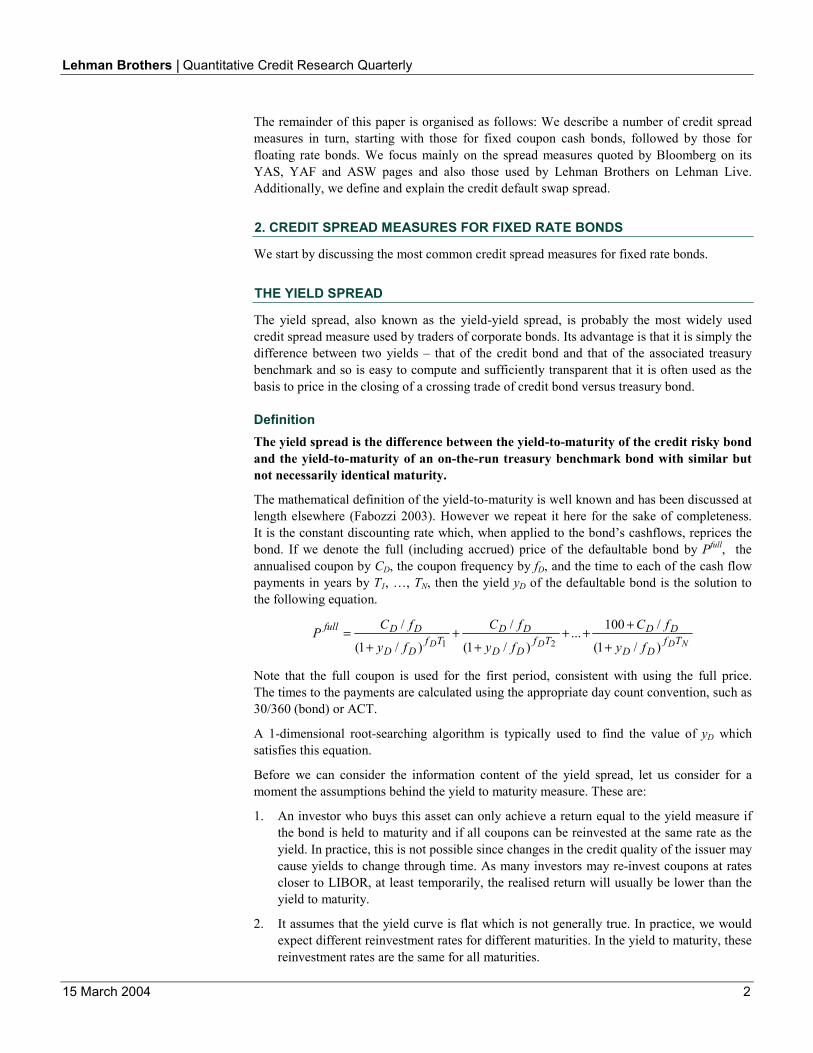
The mathematical definition of the yield-to-maturity is well known and has been discussed at length elsewhere (Fabozzi 2003). However we repeat it here for the sake of completeness. It is the constant discounting rate which, when applied to the bond’s cashflows, reprices the bond. If we denote the full (including accrued) price of the defaultable bond by Pfull, the annualised coupon by CD, the coupon frequency by fD, and the time to each of the cash flow payments in years by T1, …, TN, then the yield yD of the defaultable bond is the solution to the following equation.

NDDD TfDD

DDTf

DD

DDTf

DD

DDfull

fy

fC

fy

fC

fy

fCP)/1(

/100...)/1(

/

)/1(

/21 +

++++

++

=

Note that the full coupon is used for the first period, consistent with using the full price. The times to the payments are calculated using the appropriate day count convention, such as 30/360 (bond) or ACT.

A 1-dimensional root-searching algorithm is typically used to find the value of yD which satisfies this equation.

Before we can consider the information content of the yield spread, let us consider for a moment the assumptions behind the yield to maturity measure. These are:

1. An investor who buys this asset can only achieve a return equal to the yield measure if the bond is held to maturity and if all coupons can be reinvested at the same rate as the yield. In practice, this is not possible since changes in the credit quality of the issuer may cause yields to change through time. As many investors may re-invest coupons at rates closer to LIBOR, at least temporarily, the realised return will usually be lower than the yield to maturity.

2. It assumes that the yield curve is flat which is not generally true. In practice, we would expect different reinvestment rates for different maturities. In the yield to maturity, these reinvestment rates are the same for all maturities.


15 March 2004 3

To calculate the yield spread we also need to calculate the yield of the benchmark government bond yB as above. The yield spread is then given by the following relationship:

BD yy −=Spread Yield .

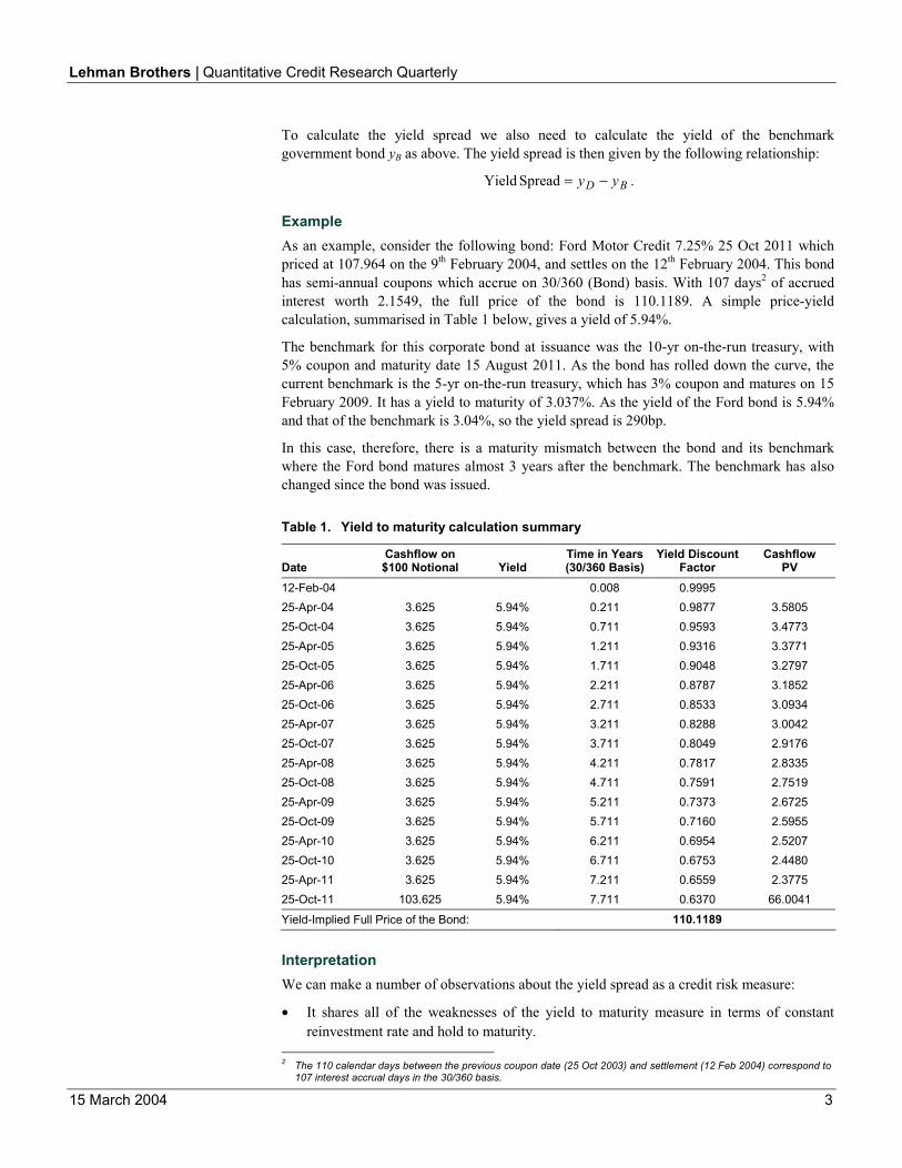
Example As an example, consider the following bond: Ford Motor Credit 7.25% 25 Oct 2011 which priced at 107.964 on the 9th February 2004, and settles on the 12th February 2004. This bond has semi-annual coupons which accrue on 30/360 (Bond) basis. With 107 days2 of accrued interest worth 2.1549, the full price of the bond is 110.1189. A simple price-yield calculation, summarised in Table 1 below, gives a yield of 5.94%.

The benchmark for this corporate bond at issuance was the 10-yr on-the-run treasury, with 5% coupon and maturity date 15 August 2011. As the bond has rolled down the curve, the current benchmark is the 5-yr on-the-run treasury, which has 3% coupon and matures on 15 February 2009. It has a yield to maturity of 3.037%. As the yield of the Ford bond is 5.94% and that of the benchmark is 3.04%, so the yield spread is 290bp.

In this case, therefore, there is a maturity mismatch between the bond and its benchmark where the Ford bond matures almost 3 years after the benchmark. The benchmark has also changed since the bond was issued.

Table 1. Yield to maturity calculation summary

Date Cashflow on $100 Notional Yield

Time in Years (30/360 Basis)

Yield Discount Factor

Cashflow PV

12-Feb-04 0.008 0.9995 25-Apr-04 3.625 5.94% 0.211 0.9877 3.5805 25-Oct-04 3.625 5.94% 0.711 0.9593 3.4773 25-Apr-05 3.625 5.94% 1.211 0.9316 3.3771 25-Oct-05 3.625 5.94% 1.711 0.9048 3.2797 25-Apr-06 3.625 5.94% 2.211 0.8787 3.1852 25-Oct-06 3.625 5.94% 2.711 0.8533 3.0934 25-Apr-07 3.625 5.94% 3.211 0.8288 3.0042 25-Oct-07 3.625 5.94% 3.711 0.8049 2.9176 25-Apr-08 3.625 5.94% 4.211 0.7817 2.8335 25-Oct-08 3.625 5.94% 4.711 0.7591 2.7519 25-Apr-09 3.625 5.94% 5.211 0.7373 2.6725 25-Oct-09 3.625 5.94% 5.711 0.7160 2.5955 25-Apr-10 3.625 5.94% 6.211 0.6954 2.5207 25-Oct-10 3.625 5.94% 6.711 0.6753 2.4480 25-Apr-11 3.625 5.94% 7.211 0.6559 2.3775 25-Oct-11 103.625 5.94% 7.711 0.6370 66.0041

Yield-Implied Full Price of the Bond: 110.1189

Interpretation We can make a number of observations about the yield spread as a credit risk measure:

• It shares all of the weaknesses of the yield to maturity measure in terms of constant reinvestment rate and hold to maturity.

2 The 110 calendar days between the previous coupon date (25 Oct 2003) and settlement (12 Feb 2004) correspond to

107 interest accrual days in the 30/360 basis.


15 March 2004 4

• Another disadvantage of being based on yield to maturity is that it is not a measure of return of a long defaultable bond, short treasury position.

• As a relative value measure, it can only be used with confidence to compare different bonds with the same maturity which may have different coupons.

• The benchmark security is chosen to have a maturity close to but not usually coincident with that of the defaultable bond. This mismatch means that the measure is biased if the underlying benchmark curve is sloped.

• The benchmark security can change over time, as the bond rolls down the curve. This is illustrated in the example above, where the bond switches from being benchmarked against a 10-yr on-the-run treasury security to a 5-yr on-the-run. As a result, yield spread is not a consistent measure through time.

The bottomline is that the yield and yield-spread measures are only rough measures of return. In no way do they actually measure the realised yield of holding the asset. For these reasons, the yield spread should only be used strictly as a way to express the price of a bond relative to the benchmark, rather than a measure of credit risk.

The only time when it may become useful is if the asset and Treasury are both trading at or very close to par. In this case, the yield to maturity of the defaultable bond and treasury are close to their coupon values and the yield spread is a measure of the annualised carry from buying the defaultable bond and shorting the Treasury. However this information is already known, so even then the yield spread does not add any value.

INTERPOLATED SPREAD

To overcome the issue of the maturity mismatch, it is possible to use a benchmark yield where the correct maturity yield has been interpolated off the appropriate reference curve. Rather than choose a specific reference benchmark bond, the idea is to use a reference yield curve which can be interpolated.

Definition The Interpolated Spread or I-spread is the difference between the yield to maturity of the bond and the linearly interpolated yield to the same maturity on an appropriate reference curve.

The simplest way to interpolate the yield off the treasury curve is to find two treasury bonds which straddle the maturity of the defaultable bond. It is then simple to linearly interpolate the yield to maturity of these two treasury bonds to find the yield corresponding to the maturity of the credit-risky bond. If the maturities of the two government bonds are TG1 and TG2 and the yields to maturity are yG1 and yG2, then the interpolated spread is given by

−

−−

+−= )( 112

121 GD

GG

GGGD TT

TTyy

yyISpread .

Other choices of reference curves include a Constant Maturity Treasury (CMT) rates curve, or the LIBOR swap rate curve. The reference curve is always specified when quoting I-spread.

Example Consider the following bond: Ford Motor Credit 7¼ 25 Oct 2011 which priced at 107.964 on the 9th February 2004, and settles on the 12th February 2004.


15 March 2004 5

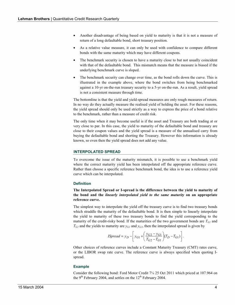
If we consider the other benchmark bonds on the US Treasury curve (shown in Figure below), we see that the two which straddle the maturity of our defaultable bond are the 3¼ Jan-09 with a yield of 3.0742% and the 4¼ Nov-13 with a yield of 4.0791%. Linearly interpolating these in maturity time gives an interpolated yield of 3.65%.

The resulting interpolated spread becomes 5.94% minus 3.65% which is 229bp. Note that this is less than the yield spread to the treasury benchmark, as the benchmark has shorter maturity than the credit bond and the treasury curve is upward-sloping.

Figure 1. I-spread against US Treasury yield curve (active)

0.00

1.00

2.00

3.00

4.00

5.00

6.00

0 2 4 6 8 10

Maturity (Years)

Yield (%)

Bond: T=7.7Y, YTM=5.94%

Active US Treasuries229bp

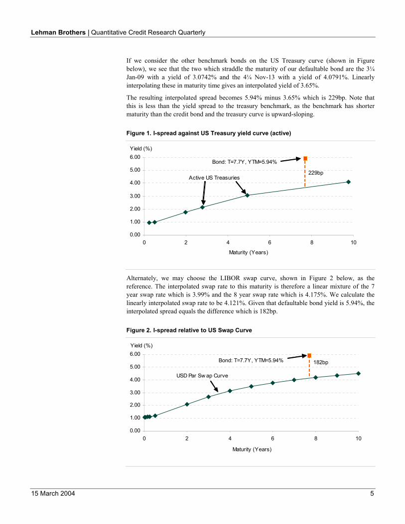
Alternately, we may choose the LIBOR swap curve, shown in Figure 2 below, as the reference. The interpolated swap rate to this maturity is therefore a linear mixture of the 7 year swap rate which is 3.99% and the 8 year swap rate which is 4.175%. We calculate the linearly interpolated swap rate to be 4.121%. Given that defaultable bond yield is 5.94%, the interpolated spread equals the difference which is 182bp.

Figure 2. I-spread relative to US Swap Curve

0.00

1.00

2.00

3.00

4.00

5.00

6.00

0 2 4 6 8 10

Maturity (Years)

Yield (%)

USD Par Sw ap Curve

Bond: T=7.7Y, YTM=5.94% 182bp


15 March 2004 6

Interpretation If the reference curve is upward sloping and the benchmark has a shorter maturity then the I-spread will be less than the yield spread. If the reference curve is downward sloping and the maturity is shorter than that of the benchmark then the I-spread will be greater than the yield spread.

Viewed purely as a yield comparison, I-spread gets around the problem of mismatched maturity which affects yield spread, but it does not necessarily correspond to the yield to maturity of a traded reference bond. In addition, it inherits all the drawbacks of the yield to maturity measure, and so should be interpreted as a way to express the price of the defaultable bond relative to a curve.

I-spread does take into account the shape of the term structure of interest rates, but only in a very crude way. The option adjusted spread, which we describe next, does so in a more robust manner.

OPTION-ADJUSTED SPREAD (OAS)

The Option Adjusted Spread (OAS) was originally conceived as a measure of the amount of optionality priced into a callable or puttable bond. However, the definition of the OAS is not option specific. Indeed it can also be used to measure the credit risk embedded in a bond.

Definition The Option Adjusted Spread is the parallel shift to the LIBOR zero rate curve required in order that the adjusted curve reprices the bond.

The OAS is sometimes referred to as the Zero-Volatility Spread (ZVS) or Z-Spread. In the latter case, semi-annual compounding is always assumed (e.g. on Bloomberg).

If we choose discrete compounding for the OAS with a frequency equal to that of the bond f, then the OAS, denoted by Ω, satisfies the following relationship:

)()(1

)()( )(

1

100)(

1

1nTf

nT

n

jjTf

jT

full

fr

frf

CP×

=×

Ω++

+

Ω++

= ∑ .

where C is the annual coupon of the bond and the LIBOR zero rates are related to LIBOR discount factors ZT as follows:

fZr TfTT ×−= ×− ]1)[( )/(1 .

In OAS calculations, time is measured as calendar time in years, rather than being dependent on the basis of the bond, as is the case with the yield to maturity calculation. A one-dimensional root-searching algorithm is used to solve this equation.

The Lehman Brothers convention, used on LehmanLive, is to use continuous compounding for the OAS, so that the above equation becomes

)()(

1

)()( 100 nT

nT

n

j

jTjT

full eZeZfCP Ω−

=

Ω− += ∑ .


15 March 2004 7

As a spread measure the OAS has a number of important differences from the yield spread. They are

1. The OAS is typically measured against LIBOR, although the reference curve is always specified and can be taken as the treasury curve as well.

2. The OAS reflects a parallel shift of the spread against LIBOR. Only the spreads are bumped rather than the whole yield. As a consequence, the OAS takes into account the shape of the term structure of LIBOR rates.

3. The OAS assumes that cashflows can be reinvested at LIBOR+OAS. As a result, future expectations about interest rates are taken into account. However there still remains reinvestment risk as it is not possible to lock in this forward rate today.

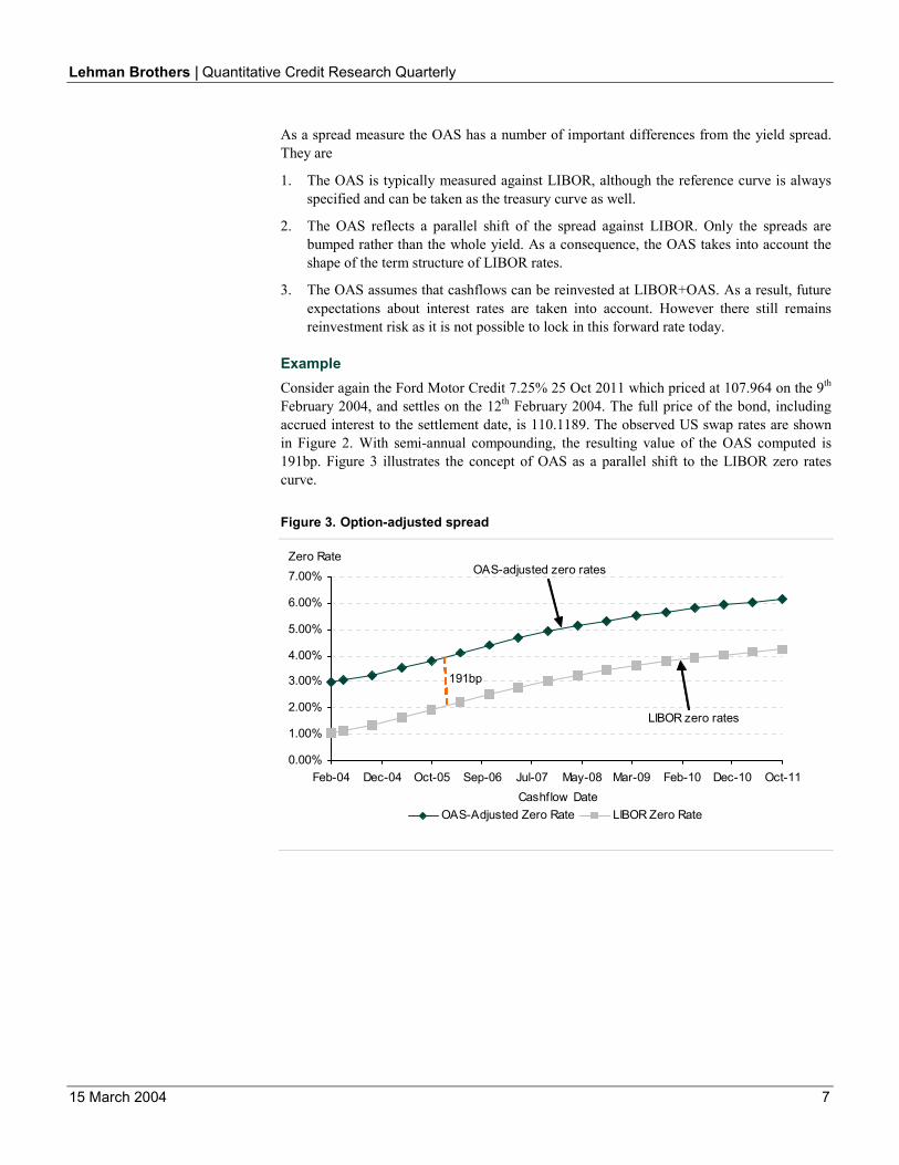
Example Consider again the Ford Motor Credit 7.25% 25 Oct 2011 which priced at 107.964 on the 9th February 2004, and settles on the 12th February 2004. The full price of the bond, including accrued interest to the settlement date, is 110.1189. The observed US swap rates are shown in Figure 2. With semi-annual compounding, the resulting value of the OAS computed is 191bp. Figure 3 illustrates the concept of OAS as a parallel shift to the LIBOR zero rates curve.

Figure 3. Option-adjusted spread

0.00%

1.00%

2.00%

3.00%

4.00%

5.00%

6.00%

7.00%

Feb-04 Dec-04 Oct-05 Sep-06 Jul-07 May-08 Mar-09 Feb-10 Dec-10 Oct-11

Zero Rate

OAS-Adjusted Zero Rate LIBOR Zero RateCashflow Date

OAS-adjusted zero rates

LIBOR zero rates

191bp


15 March 2004 8

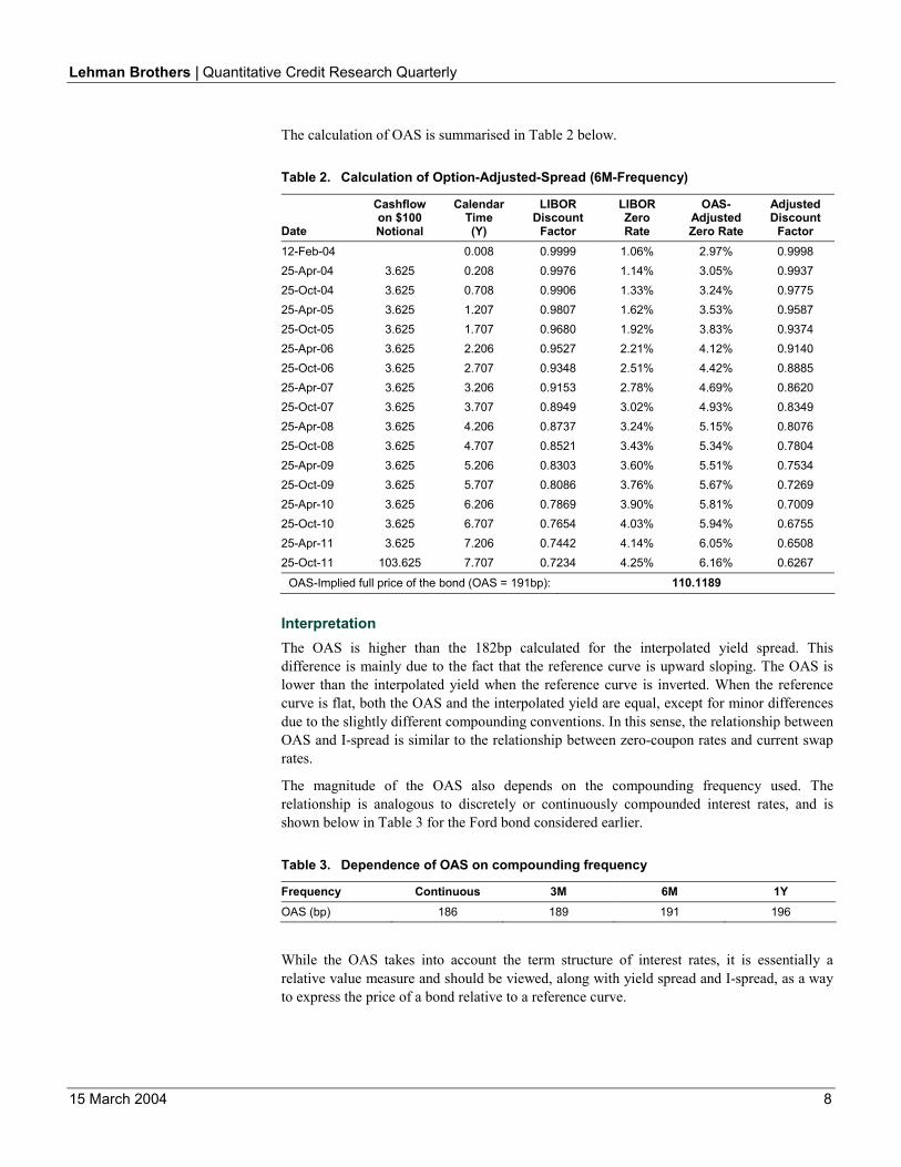
The calculation of OAS is summarised in Table 2 below.

Table 2. Calculation of Option-Adjusted-Spread (6M-Frequency)

Date

Cashflow on $100 Notional

Calendar Time (Y)

LIBOR Discount

Factor

LIBOR Zero Rate

OAS-Adjusted Zero Rate

Adjusted Discount

Factor 12-Feb-04 0.008 0.9999 1.06% 2.97% 0.9998 25-Apr-04 3.625 0.208 0.9976 1.14% 3.05% 0.9937 25-Oct-04 3.625 0.708 0.9906 1.33% 3.24% 0.9775 25-Apr-05 3.625 1.207 0.9807 1.62% 3.53% 0.9587 25-Oct-05 3.625 1.707 0.9680 1.92% 3.83% 0.9374 25-Apr-06 3.625 2.206 0.9527 2.21% 4.12% 0.9140 25-Oct-06 3.625 2.707 0.9348 2.51% 4.42% 0.8885 25-Apr-07 3.625 3.206 0.9153 2.78% 4.69% 0.8620 25-Oct-07 3.625 3.707 0.8949 3.02% 4.93% 0.8349 25-Apr-08 3.625 4.206 0.8737 3.24% 5.15% 0.8076 25-Oct-08 3.625 4.707 0.8521 3.43% 5.34% 0.7804 25-Apr-09 3.625 5.206 0.8303 3.60% 5.51% 0.7534 25-Oct-09 3.625 5.707 0.8086 3.76% 5.67% 0.7269 25-Apr-10 3.625 6.206 0.7869 3.90% 5.81% 0.7009 25-Oct-10 3.625 6.707 0.7654 4.03% 5.94% 0.6755 25-Apr-11 3.625 7.206 0.7442 4.14% 6.05% 0.6508 25-Oct-11 103.625 7.707 0.7234 4.25% 6.16% 0.6267

OAS-Implied full price of the bond (OAS = 191bp): 110.1189

Interpretation The OAS is higher than the 182bp calculated for the interpolated yield spread. This difference is mainly due to the fact that the reference curve is upward sloping. The OAS is lower than the interpolated yield when the reference curve is inverted. When the reference curve is flat, both the OAS and the interpolated yield are equal, except for minor differences due to the slightly different compounding conventions. In this sense, the relationship between OAS and I-spread is similar to the relationship between zero-coupon rates and current swap rates.

The magnitude of the OAS also depends on the compounding frequency used. The relationship is analogous to discretely or continuously compounded interest rates, and is shown below in Table 3 for the Ford bond considered earlier.

Table 3. Dependence of OAS on compounding frequency

Frequency Continuous 3M 6M 1Y OAS (bp) 186 189 191 196

While the OAS takes into account the term structure of interest rates, it is essentially a relative value measure and should be viewed, along with yield spread and I-spread, as a way to express the price of a bond relative to a reference curve.


15 March 2004 9

ASSET SWAP SPREAD (ASW)

Unlike the spread measures described so far, the asset swap spread is a traded spread rather than an artificial measure of credit spread.

Definition The Asset swap spread is the spread over LIBOR paid on the floating leg in a par asset swap package.

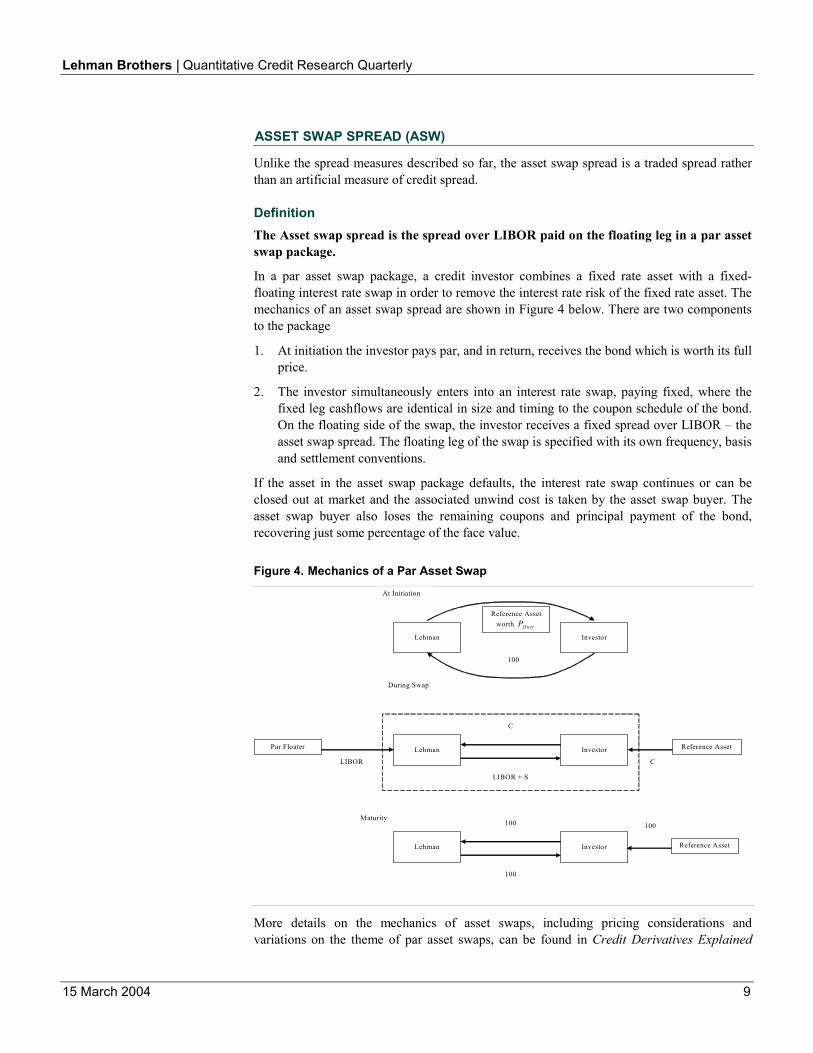
In a par asset swap package, a credit investor combines a fixed rate asset with a fixed-floating interest rate swap in order to remove the interest rate risk of the fixed rate asset. The mechanics of an asset swap spread are shown in Figure 4 below. There are two components to the package

1. At initiation the investor pays par, and in return, receives the bond which is worth its full price.

2. The investor simultaneously enters into an interest rate swap, paying fixed, where the fixed leg cashflows are identical in size and timing to the coupon schedule of the bond. On the floating side of the swap, the investor receives a fixed spread over LIBOR – the asset swap spread. The floating leg of the swap is specified with its own frequency, basis and settlement conventions.

If the asset in the asset swap package defaults, the interest rate swap continues or can be closed out at market and the associated unwind cost is taken by the asset swap buyer. The asset swap buyer also loses the remaining coupons and principal payment of the bond, recovering just some percentage of the face value.

Figure 4. Mechanics of a Par Asset Swap

Lehman

100

Investor

Lehman

Investor

Reference Asset worth DirtyP

C

Reference Asset

LIBOR + S

C

Lehman

Investor

100

100

Maturity

Par Floater

LIBOR

At Initiation

During Swap

Reference Asset

100

More details on the mechanics of asset swaps, including pricing considerations and variations on the theme of par asset swaps, can be found in Credit Derivatives Explained


15 March 2004 10

(March 2001), and Tuckman (2003), where we show that the par asset swap spread is given by the formula:

01PVPPA

fullLIBOR −=

Equation 1

Here, PLIBOR is the value of the bond’s cashflows discounted at LIBOR, Pfull is the market price of the bond, and PV01 is the LIBOR discounted present value of a 1bp coupon stream, paid according to the frequency, basis and stub conventions of the floating leg of the interest rate swap.

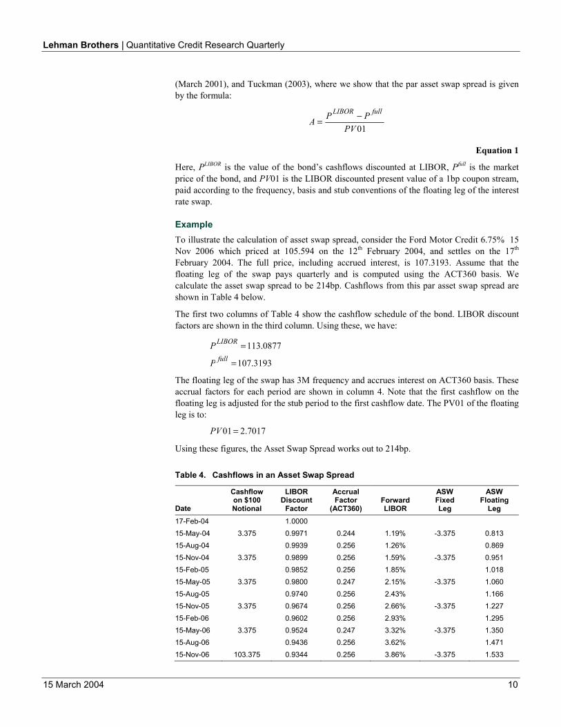
Example To illustrate the calculation of asset swap spread, consider the Ford Motor Credit 6.75% 15 Nov 2006 which priced at 105.594 on the 12th February 2004, and settles on the 17th February 2004. The full price, including accrued interest, is 107.3193. Assume that the floating leg of the swap pays quarterly and is computed using the ACT360 basis. We calculate the asset swap spread to be 214bp. Cashflows from this par asset swap spread are shown in Table 4 below.

The first two columns of Table 4 show the cashflow schedule of the bond. LIBOR discount factors are shown in the third column. Using these, we have:

3193.107

0877.113

=

=full

LIBOR

P

P

The floating leg of the swap has 3M frequency and accrues interest on ACT360 basis. These accrual factors for each period are shown in column 4. Note that the first cashflow on the floating leg is adjusted for the stub period to the first cashflow date. The PV01 of the floating leg is to:

7017.201 =PV

Using these figures, the Asset Swap Spread works out to 214bp.

Table 4. Cashflows in an Asset Swap Spread

Date

Cashflow on $100 Notional

LIBOR Discount

Factor

Accrual Factor

(ACT360) Forward LIBOR

ASW Fixed Leg

ASW Floating

Leg 17-Feb-04 1.0000 15-May-04 3.375 0.9971 0.244 1.19% -3.375 0.813 15-Aug-04 0.9939 0.256 1.26% 0.869 15-Nov-04 3.375 0.9899 0.256 1.59% -3.375 0.951 15-Feb-05 0.9852 0.256 1.85% 1.018 15-May-05 3.375 0.9800 0.247 2.15% -3.375 1.060 15-Aug-05 0.9740 0.256 2.43% 1.166 15-Nov-05 3.375 0.9674 0.256 2.66% -3.375 1.227 15-Feb-06 0.9602 0.256 2.93% 1.295 15-May-06 3.375 0.9524 0.247 3.32% -3.375 1.350 15-Aug-06 0.9436 0.256 3.62% 1.471 15-Nov-06 103.375 0.9344 0.256 3.86% -3.375 1.533


15 March 2004 11

Interpretation One thing to understand about the asset swap spread is that if the asset in the asset swap defaults immediately after initiation, the investor, who has paid 100 for the asset swap, is left with an asset which can be sold for a recovery price R, and an interest rate swap worth 100-P where P is the full price of the bond at initiation. The loss to the investor is -100-R-(100-P) = P-R, the difference between the full price of the bond and the recovery price of the defaulted bond. If the price of the asset is par, i.e. P = 100, then the loss on immediate default is 100-R, similar as we shall see to a default swap.

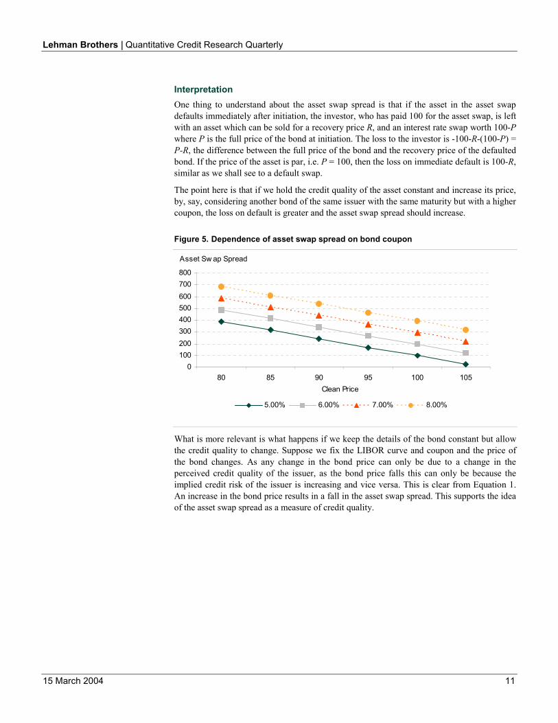
The point here is that if we hold the credit quality of the asset constant and increase its price, by, say, considering another bond of the same issuer with the same maturity but with a higher coupon, the loss on default is greater and the asset swap spread should increase.

Figure 5. Dependence of asset swap spread on bond coupon

0100200300400500600700800

80 85 90 95 100 105Clean Price

5.00% 6.00% 7.00% 8.00%

Asset Sw ap Spread

What is more relevant is what happens if we keep the details of the bond constant but allow the credit quality to change. Suppose we fix the LIBOR curve and coupon and the price of the bond changes. As any change in the bond price can only be due to a change in the perceived credit quality of the issuer, as the bond price falls this can only be because the implied credit risk of the issuer is increasing and vice versa. This is clear from Equation 1. An increase in the bond price results in a fall in the asset swap spread. This supports the idea of the asset swap spread as a measure of credit quality.


15 March 2004 12

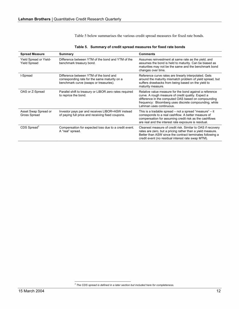
Table 5 below summarises the various credit spread measures for fixed rate bonds.

Table 5. Summary of credit spread measures for fixed rate bonds

Spread Measure Summary Comments Yield Spread or Yield-Yield Spread

Difference between YTM of the bond and YTM of the benchmark treasury bond.

Assumes reinvestment at same rate as the yield, and assumes the bond is held to maturity. Can be biased as maturities may not be the same and the benchmark bond changes over time.

I-Spread Difference between YTM of the bond and corresponding rate for the same maturity on a benchmark curve (swaps or treasuries).

Reference curve rates are linearly interpolated. Gets around the maturity mismatch problem of yield spread, but suffers drawbacks from being based on the yield to maturity measure.

OAS or Z-Spread Parallel shift to treasury or LIBOR zero rates required to reprice the bond.

Relative value measure for the bond against a reference curve. A rough measure of credit quality. Expect a difference in the computed OAS based on compounding frequency: Bloomberg uses discrete compounding, while Lehman uses continuous.

Asset Swap Spread or Gross Spread

Investor pays par and receives LIBOR+ASW instead of paying full price and receiving fixed coupons.

This is a tradable spread – not a spread “measure” – it corresponds to a real cashflow. A better measure of compensation for assuming credit risk as the cashflows are real and the interest rate exposure is residual.

CDS Spread3 Compensation for expected loss due to a credit event. A “real” spread.

Cleanest measure of credit risk. Similar to OAS if recovery rates are zero, but a pricing rather than a yield measure. Better than ASW since the contract terminates following a credit event (no residual interest rate swap MTM).

3 The CDS spread is defined in a later section but included here for completeness.


15 March 2004 13

3. CREDIT SPREAD MEASURES FOR FLOATING RATE NOTES

We now turn to Floating Rate Notes (FRNs). In contrast to fixed rate bonds, there are fewer commonly quoted measures of spread for FRNs. These are the quoted margin which determines contractual cashflows, discount margin which is similar to yield-to-maturity, and zero-discount margin which is similar to OAS. We now describe each in turn.

QUOTED MARGIN (QM)

The quoted margin is not strictly a spread measure; it is simply the spread over the LIBOR index paid by a floating rate note.

Definition The quoted margin is the fixed, contractual spread over the floating rate index, usually LIBOR, paid by a floating rate note.

Once issued, the quoted margin of the bond is contractually fixed. In certain cases, defined within the bond prospectus, it may step up or down. It is therefore not a dynamic measure of ongoing credit quality. At most it only reflects the credit quality of the issuer on the issue date of the bond since this was the spread over LIBOR at which the bond could be issued at par

Example To illustrate credit spread measures for FRN’s, we consider a Ford Motor Credit bond with maturity 6 January 2006. This bond pays quarterly coupons indexed to the 3M-Euribor with accrued interest computed on an ACT360 basis. It is currently trading at a clean price of 101.09.

The quoted margin for this bond is 175bp. The floating rate is set at the start of each period, so that the coupon is known 3 months in advance. In this case, the size of the coupon due on 6 April 2004 is 3.87% (annualised), which means that the floating rate was fixed at 2.12% on 6 January 2004.

DISCOUNT MARGIN (DM)

Unlike the quoted margin, the discount margin is a dynamic spread measure which reflects the ongoing perceived credit quality of the note issuer. It is a simple measure of spread which assumes that the underlying reference curve is flat.

Definition The discount margin is the fixed add-on to the current LIBOR rate that is required to reprice the bond.

Discount margin measures yield relative to the current LIBOR level and does not take into account the term structure of interest rates. In this sense, it is analogous to the YTM of a fixed rate bond.

The expected cashflows of an FRN are usually based on forward LIBOR rates. In the discount margin calculation, however, the assumption is that all future realised LIBOR rates will be equal to the current LIBOR rate. Cashflows are therefore projected as the current LIBOR plus quoted margin (except for the first cashflow, which is known for sure). Discount


15 March 2004 14

factors are also based on the current level of LIBOR, adjusted by a margin. The size of the margin is chosen to reprice the FRN, in which case it is called the discount margin.

The discount margin δ satisfies the following relationship:

)(100)()()(1 21

n

n

jjj

stub

fixfull TZqLTZL

qLP δ

=δ ++∆+

δ+∆+

+= ∑

where

)(11)(;

)(1)(

)(1

11

δ+∆+=

δ+∆+= δ

−δδ

stubj

jj L

TZL

TZTZ

and we have used the following notation:

Pfull = Full price of the FRN

q = Quoted margin on the FRN

Lfix = Known LIBOR rate for the current coupon period

Lstub = LIBOR between the valuation date and the next coupon date

L = Current LIBOR for the term of the FRN coupons (e.g. 3M)

∆1,…,∆n = Coupon accrual periods in the appropriate basis (e.g. ACT360)

T1,…,Tn = Cashflow dates for the FRN

This calculation assumes that all future LIBOR cash flows are equal to the previous fixing. As a result, no account is taken of the shape of the LIBOR forward curve as in the par floater calculation.

Example The concept of discount margin is best illustrated using an example. Consider the same bond as before, i.e. Ford €+175bp 6 Jan 2006. The previous Euribor fixing, which together with the quoted margin determines the cashflow at the next coupon date, is 2.12%. The stub Euribor to the next coupon date, used to determine the discount factor, is 2.057%.

The bond pays quarterly coupons. The current level of 3M-Euribor is 2.064%. For all cashflows beyond the next coupon date to maturity, the discount margin calculation assumes that the realised Euribor rate is equal to 2.064%. This is also used in discounting.

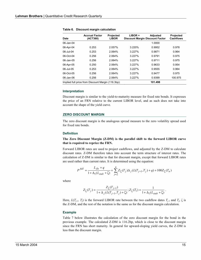
The calculation of discount margin is illustrated in Table 6. Since the Euribor fixing for the current period is known, we can compute accrued interest. The full price of the FRN is 101.50. The discount margin comes out to 116.3bp.

As with most spread calculations for fixed rate bonds, we typically need to use a 1-dimensional root-searching algorithm to solve for the discount margin.


15 March 2004 15

Table 6. Discount margin calculation

Date Accrual Factor

(ACT360) Projected

LIBOR LIBOR +

Discount Margin Adjusted

Discount FactorProjected Cashflows

06-Jan-04 1.0000 06-Apr-04 0.253 2.057% 3.220% 0.9952 0.978 06-Jul-04 0.253 2.064% 3.227% 0.9871 0.964 06-Oct-04 0.256 2.064% 3.227% 0.9791 0.975 06-Jan-05 0.256 2.064% 3.227% 0.9711 0.975 06-Apr-05 0.250 2.064% 3.227% 0.9633 0.954 06-Jul-05 0.253 2.064% 3.227% 0.9555 0.964 06-Oct-05 0.256 2.064% 3.227% 0.9477 0.975 06-Jan-06 0.256 2.064% 3.227% 0.9399 100.975

Implied full price from Discount Margin (116.3bp): 101.498

Interpretation Discount margin is similar to the yield-to-maturity measure for fixed rate bonds. It expresses the price of an FRN relative to the current LIBOR level, and as such does not take into account the shape of the yield curve.

ZERO DISCOUNT MARGIN

The zero discount margin is the analogous spread measure to the zero volatility spread used for fixed rate bonds.

Definition The Zero Discount Margin (Z-DM) is the parallel shift to the forward LIBOR curve that is required to reprice the FRN.

Forward LIBOR rates are used to project cashflows, and adjusted by the Z-DM to calculate discount rates. Z-DM therefore takes into account the term structure of interest rates. The calculation of Z-DM is similar to that for discount margin, except that forward LIBOR rates are used rather than current rates. It is determined using the equation:

)(100)),(()()(1 2

11

n

n

jjjjj

stub

fixfull TZqTTLTZL

qLP ζ

=−ζ ++∆+

ζ+∆++

= ∑

where

)(11)(;

)),((1)(

)(1

11

1

ζ+∆+=

ζ+∆+= ζ

−

−ζζ

stubjjj

jj L

TZTTL

TZTZ .

Here, L(Tj-1, Tj) is the forward LIBOR rate between the two cashflow dates Tj-1 and Tj, ζ is the Z-DM, and the rest of the notation is the same as for the discount margin calculation.

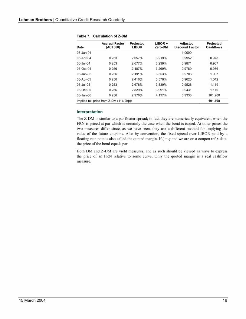
Example Table 7 below illustrates the calculation of the zero discount margin for the bond in the previous example. The calculated Z-DM is 116.2bp, which is close to the discount margin since the FRN has short maturity. In general for upward-sloping yield curves, the Z-DM is less than the discount margin.


15 March 2004 16

Table 7. Calculation of Z-DM

Date Accrual Factor

(ACT360) Projected

LIBOR LIBOR + Zero-DM

Adjusted Discount Factor

Projected Cashflows

06-Jan-04 1.0000 06-Apr-04 0.253 2.057% 3.219% 0.9952 0.978 06-Jul-04 0.253 2.077% 3.239% 0.9871 0.967 06-Oct-04 0.256 2.107% 3.269% 0.9789 0.986 06-Jan-05 0.256 2.191% 3.353% 0.9706 1.007 06-Apr-05 0.250 2.416% 3.578% 0.9620 1.042 06-Jul-05 0.253 2.678% 3.839% 0.9528 1.119 06-Oct-05 0.256 2.829% 3.991% 0.9431 1.170 06-Jan-06 0.256 2.976% 4.137% 0.9333 101.208

Implied full price from Z-DM (116.2bp): 101.498

Interpretation The Z-DM is similar to a par floater spread; in fact they are numerically equivalent when the FRN is priced at par which is certainly the case when the bond is issued. At other prices the two measures differ since, as we have seen, they use a different method for implying the value of the future coupons. Also by convention, the fixed spread over LIBOR paid by a floating rate note is also called the quoted margin. If ζ = q and we are on a coupon refix date, the price of the bond equals par.

Both DM and Z-DM are yield measures, and as such should be viewed as ways to express the price of an FRN relative to some curve. Only the quoted margin is a real cashflow measure.


15 March 2004 17

4. CREDIT DEFAULT SWAP SPREAD

The CDS spread is the contractual premium paid to a protection seller in a credit default swap contract. As such it measures the compensation to an investor for taking on the risk of losing par minus the expected recovery rate of a bond if a credit event occurs before the maturity of the CDS contract. It is termed a “spread” even though it does not explicitly reference any interest rate curve. However, implicitly, the reference curve is Libor.

Definition The CDS spread is the contractual spread which determines the cashflows paid on the premium leg of a credit default swap.

It is the spread which makes the expected present value of the protection and premium legs the same. The valuation of CDS is described fully in the references and reviewed in the next section, but we can consider a simple example to explain the basic concepts.

Example Suppose an investor sells protection on $10mm notional to a 5-year horizon on a credit risky issuer at a default swap spread of 200bp. The investor is paid for protection in the form of fixed quarterly instalments of approximately $50,000. The payments stop if the issuer defaults prior to maturity, in which case the value of protection delivered by the seller is par minus the recovery rate. Assuming a recovery rate of 40%, the investor would lose $6mm.

It has been shown that the valuation of a CDS position requires a model. The reader is referred to O’Kane and Turnbull (2003) for a more detailed discussion.

Interpretation The CDS spread is arguably the best measure of credit risk for several reasons. First, a CDS contract is almost a pure credit play, with low interest rate risk. Second, it corresponds to a realisable stream of cashflows, which compensates an investor for a loss of par minus the recovery rate of the issuer following a credit event. All cashflows cease and the contract is settled following a credit event. Third, an investor can trade CDS to a number of fixed terms, so we should be able to observe a term structure. Finally, the CDS market is relatively liquid, so that CDS spreads accurately reflect the market price of credit risk.

5. CONCLUSIONS

In this article, we have tried to explain the precise definition and significance of the plethora of market terms used to express the credit risk embedded in a bond. There is an important distinction between measures of yield and tradable measures of spread. The former should be viewed as convenient ways to express the price of a bond or FRN relative to some benchmark instrument (bond, rate or curve). The latter can be translated into physical cashflows. There remains the important issue of how these spreads compare with each other, particularly in regard to their relative magnitudes and sensitivities to changes in the credit quality of the underlying bond. This analysis is left to a forthcoming paper in the Quantitative Credit Research Quarterly series.


15 March 2004 18

6. REFERENCES

1. Tuckman, B.: “Measures of Asset Swap Spread and their Corresponding Trades”. Lehman Brothers Fixed Income Research, January 2003.

2. Fabozzi, F. (ed.): “The Handbook of Fixed Income Securities”. Wiley, 2003.

3. McAdie, R. and O’Kane, D.: “Explaining the Basis: Cash Versus Default Swaps”. Lehman Brothers Structured Credit Research, May 2001.

4. Naldi, M., O’Kane, D., et al.: “The Lehman Brothers Guide to Exotic Credit Derivatives”. Special supplement to Risk magazine, October 2003.

5. O’Kane, D.: “Credit Derivatives Explained”. Lehman Brothers Structured Credit Research, March 2001.

6. O’Kane, D. and Schloegl, L.: “Modelling Credit – Theory and Practice”. Lehman Brothers Analytical Research Series, February 2001.

This material has been prepared and/or issued by Lehman Brothers Inc., member SIPC, and/or one of its affiliates (“Lehman Brothers”) and has been approved by Lehman BrothersInternational (Europe), regulated by the Financial Services Authority, in connection with its distribution in the European Economic Area. This material is distributed in Japan by LehmanBrothers Japan Inc., and in Hong Kong by Lehman Brothers Asia Limited. This material is distributed in Australia by Lehman Brothers Australia Pty Limited, and in Singapore by LehmanBrothers Inc., Singapore Branch. This document is for information purposes only and it should not be regarded as an offer to sell or as a solicitation of an offer to buy the securities orother instruments mentioned in it. No part of this document may be reproduced in any manner without the written permission of Lehman Brothers. We do not represent that thisinformation, including any third party information, is accurate or complete and it should not be relied upon as such. It is provided with the understanding that Lehman Brothers is notacting in a fiduciary capacity. Opinions expressed herein reflect the opinion of Lehman Brothers and are subject to change without notice. The products mentioned in this documentmay not be eligible for sale in some states or countries, and they may not be suitable for all types of investors. If an investor has any doubts about product suitability, he should consulthis Lehman Brothers’ representative. The value of and the income produced by products may fluctuate, so that an investor may get back less than he invested. Value and income maybe adversely affected by exchange rates, interest rates, or other factors. Past performance is not necessarily indicative of future results. If a product is income producing, part of thecapital invested may be used to pay that income. Lehman Brothers may make a market or deal as principal in the securities mentioned in this document or in options, futures, or otherderivatives based thereon. In addition, Lehman Brothers, its shareholders, directors, officers and/or employees, may from time to time have long or short positions in such securities or inoptions, futures, or other derivative instruments based thereon. One or more directors, officers, and/or employees of Lehman Brothers may be a director of the issuer of the securitiesmentioned in this document. Lehman Brothers may have managed or co-managed a public offering of securities for any issuer mentioned in this document within the last three years,or may, from time to time, perform investment banking or other services for, or solicit investment banking or other business from any company mentioned in this document.

2004 Lehman Brothers. All rights reserved.Additional information is available on request. Please contact a Lehman Brothers’ entity in your home jurisdiction.

Lehman Brothers Fixed Income Research analysts produce proprietary research in conjunction with firm trading desks that trade as principal in the instrumentsmentioned herein, and hence their research is not independent of the proprietary interests of the firm. The firm’s interests may conflict with the interests of aninvestor in those instruments.Lehman Brothers Fixed Income Research analysts receive compensation based in part on the firm’s trading and capital markets revenues. Lehman Brothers andany affiliate may have a position in the instruments or the company discussed in this report.The views expressed in this report accurately reflect the personal views of Dominic O’Kane and Saurav Sen, the primary analyst(s) responsible for this report,about the subject securities or issuers referred to herein, and no part of such analyst(s)’ compensation was, is or will be directly or indirectly related to the specificrecommendations or views expressed herein.The research analysts responsible for preparing this report receive compensation based upon various factors, including, among other things, the quality of theirwork, firm revenues, including trading and capital markets revenues, competitive factors and client feedback.

To the extent that any of the views expressed in this research report are based on the firm’s quantitative research model, Lehman Brothers hereby certify (1) thatthe views expressed in this research report accurately reflect the firm’s quantitative research model and (2) that no part of the firm’s compensation was, is or will bedirectly or indirectly related to the specific recommendations or views expressed in this report.

Any reports referenced herein published after 14 April 2003 have been certified in accordance with Regulation AC. To obtain copies of these reports and their certifications,please contact Larry Pindyck ([email protected]; 212-526-6268) or Valerie Monchi ([email protected]; 44-207-102-8035).

Credit Spreads Explained

Documents

Transcript of Credit Spreads Explained