1

Credit Spread Arbitrage in Emerging Eurobond Markets

Caio Ibsen Rodrigues de Almeida *,a Antonio Marcos Duarte, Jr. **

Cristiano Augusto Coelho Fernandes ***

Abstract Simulating the movements of term structures of interest rates plays an important role when optimally allocating portfolios in fixed income markets. These movements allow the generation of scenarios that provide the assets’ sensitivity to the fluctuation of interest rates. The problem becomes even more interesting when the portfolio is international. In this case, there is a need to synchronize the different scenarios for the movements of the interest rate curves in each country. An important factor to consider, in this context, is credit risk. For instance, in the corporate Emerging Eurobond fixed income market there are two main sources of credit risk: sovereign risk and the relative credit among the companies issuers of the eurobonds. This article presents a model to estimate, in a one step procedure, both the term structure of interest rates and the credit spread function of a diversified international portfolio of eurobonds, with different credit ratings. The estimated term structures can be used to analyze credit spread arbitrage opportunities in Eurobond markets. Numerical examples taken from the Argentinean, Brazilian and Mexican Eurobond markets are presented to illustrate the practical use of the methodology.

Please address all correspondence to: Antonio Marcos Duarte, Jr., Director

Risk Management Unibanco S.A.

Av. Eusébio Matoso, 891 / 5 andar 05423-901 São Paulo, SP, Brazil

Phone: 55-11-30971668 Fax: 55-11-30974276

a The first author acknowledges the financial support granted by FAPERJ

* Pontifícia Universidade Católica do Rio de Janeiro, Brazil. E-mail: caio@ele.puc-rio.br ** Unibanco S.A., Brazil. E-mail: antonio.duarte@unibanco.com.br *** Pontifícia Universidade Católica do Rio de Janeiro, Brazil. E-mail: cris@ele.puc-rio.br

2

1. Introduction

The prices of fixed income assets depend on three components (Litterman

and Iben [1988]): the risk free term structure of interest rates, embedded options

values and credit risk. Optimally allocating portfolios in fixed income markets

demands a detailed analysis of each of these components.

Several authors have already considered the risk free term structure

estimation problem. For example, Vasicek and Fong [1982] suggest a statistical

model based on exponential splines. Litterman and Scheinkman [1991] verified that

there are three orthogonal factors which explain the majority of the movements of the

US term structure of interest rates. These three factors form the basis for many fixed

income pricing and hedging applications. For instance, these factors are used in Singh

[1997] to suggest optimal hedges.

Some bonds present embedded options. In general, the price of an embedded

option is a nonlinear function of its underlying bond price on all dates before the

option maturity date. An embedded option depends not only on the actual term

structure of interest rates, but also on the evolution of this term structure during the

life of the option. Several models have been proposed for the evolution of the term

structure of interest rates. These models are classified in two major groups (Heath et

al. [1992]): equilibrium models (Cox et al. [1985], among others) and arbitrage free

models (Heath et al. [1992], Ho and Lee [1986], Vasicek [1977], among others). At

this point in time, the pricing of embedded options using arbitrage free models is

perceived as the most appropriate because the parameters can be chosen to be

consistent with the actual term structure of interest rates and, consequently, to the

actual prices of bonds (Heath et al. [1992]). The process modeled can be the short-

term interest rate, the whole term structure of interest rates, or the forward rates

curve. No matter what the process is, when it is Markovian, it is usually implemented

using binomial trees (Black et al. [1990]) or trinomial trees (Hull and White [1993]).

Almeida et al. [1998] presented a model to decompose the credit risk of term

structures of interest rates using orthogonal factors, such as Legendre polynomials

(Sansone [1959]). In this model, the term structure of interest rates is decomposed in

3

two curves: a benchmark curve and a credit spread function. The last one is modeled

using a linear combination of Legendre polynomials.

In this article we present a model to estimate, in a single step, both the term

structure of interest rates and the credit spread function of an international portfolio of

bonds with different credit ratings. This model extends the approach proposed in

Almeida et al [1998]. It allows the joint estimation of the credit spread function of

any international portfolio with different credit ratings. This extension is crucial when

analyzing credit spread arbitrage opportunities in fixed income markets. For the

purpose of illustration, we concentrate on the Emerging Corporate Eurobond market,

studying the three most important in Latin America: Argentina, Brazil and Mexico.

However, the methodology is quite general, and can be applied to any fixed income

portfolio composed by bonds with different credit ratings.

This article is organized as follows. Section 2 explains the model. Section 3

presents the estimation process for its parameters. Section 4 explains the methodology

used for optimally allocating portfolios using the model. Section 5 presents three

practical examples of detection and exploitation of arbitrage opportunities in the Latin

American Eurobond market. Section 6 presents a summary of the article, and the

conclusions.

2. The Model

Suppose we want to analyze a portfolio in the Emerging Eurobond market.

Assets with the same cash flow and embedded option structures, but different credit

ratings, ought to have different prices. For this reason, when structuring fixed income

portfolios, it is fundamental to estimate and simulate the movements of different term

structures of interest rates, one for each credit rating in the portfolio. One possibility

would be to estimate a term structure, for each credit rating. There is a statistical

problem with the amount of data available when relying on this approach: in the

emerging eurobond market there are usually very few liquid bonds for each credit

rating. A joint estimation procedure is thus necessary.

4

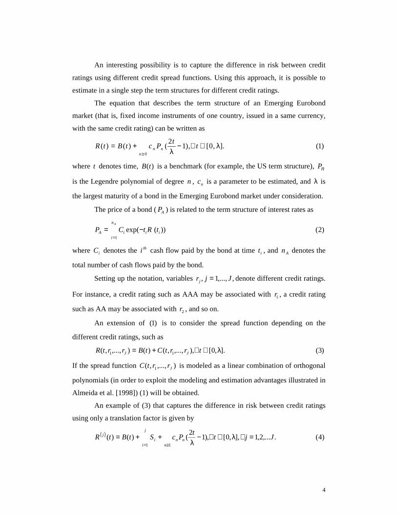
An interesting possibility is to capture the difference in risk between credit

ratings using different credit spread functions. Using this approach, it is possible to

estimate in a single step the term structures for different credit ratings.

The equation that describes the term structure of an Emerging Eurobond

market (that is, fixed income instruments of one country, issued in a same currency,

with the same credit rating) can be written as

)1( ].,0[,)12()()(0

λλ

∈∀−+=≥

ttPctBtR nn

n

where t denotes time, )(tB is a benchmark (for example, the US term structure), nP

is the Legendre polynomial of degree n , nc is a parameter to be estimated, and λ is

the largest maturity of a bond in the Emerging Eurobond market under consideration.

The price of a bond ( AP ) is related to the term structure of interest rates as

)2( ))(exp(1=

−=An

iiiiA tRtCP

where iC denotes the thi cash flow paid by the bond at time it , and An denotes the

total number of cash flows paid by the bond.

Setting up the notation, variables ,,...,1, Jjrj = denote different credit ratings.

For instance, a credit rating such as AAA may be associated with 1r , a credit rating

such as AA may be associated with 2r , and so on.

An extension of )1( is to consider the spread function depending on the

different credit ratings, such as

)3( ].,0[),,...,,()(),...,,( 11 λ∈∀+= trrtCtBrrtR JJ

If the spread function ),...,,( 1 JrrtC is modeled as a linear combination of orthogonal

polynomials (in order to exploit the modeling and estimation advantages illustrated in

Almeida et al. [1998]) (1) will be obtained.

An example of (3) that captures the difference in risk between credit ratings

using only a translation factor is given by

( ) )4( .,...2,1],,0[,)12()()(11

JjttPcStBtR nn

n

j

ii

j =∀∈∀−++=≥=

λλ

5

where iS is a nonnegative spread variable (that is, jiSi ,...,2,1 0 =∀≥ ) that measures

the difference in risk between the thi )1( − and the thi credit ratings, and J represents

the total number of credit ratings.

A limitation of )4( is that all J estimated term structures are parallel.

Although very limited, )4( captures the fact that bonds with “better” ratings ought to

have smaller prices (everything else being equal). In other words: the “better” the

rating, the higher the interest rates used to price bonds with that particular rating.

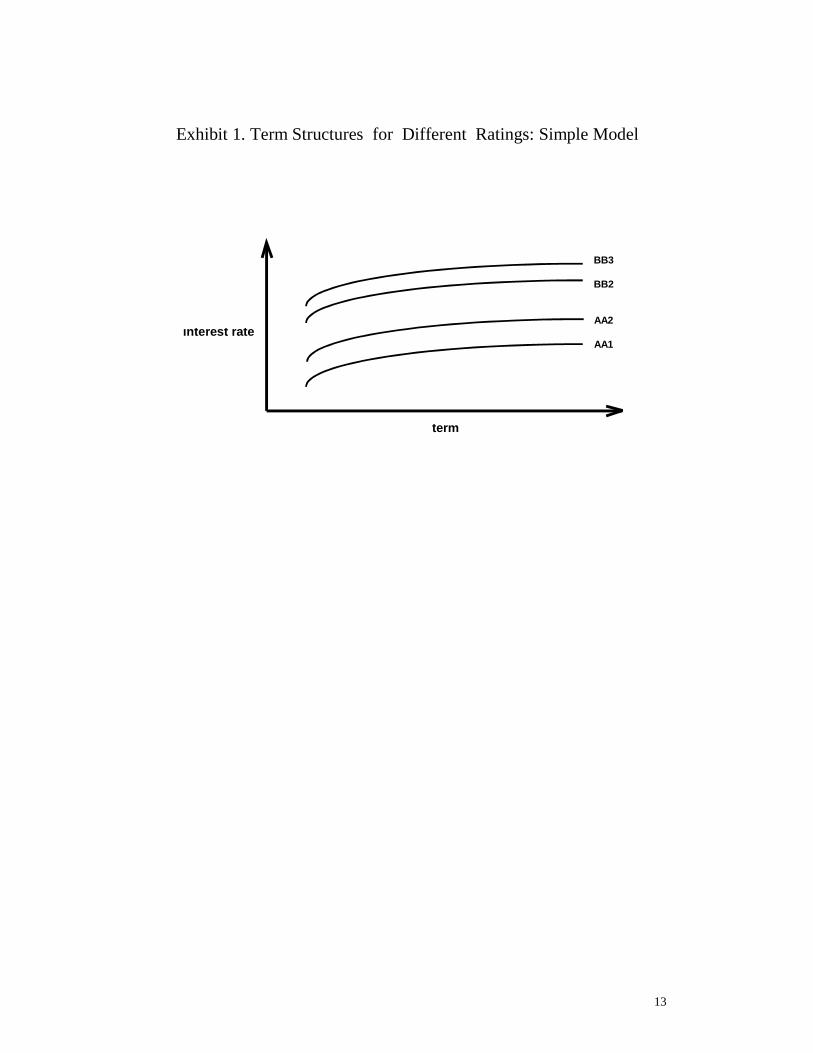
Exhibit 1 depicts a possible output for )4( .

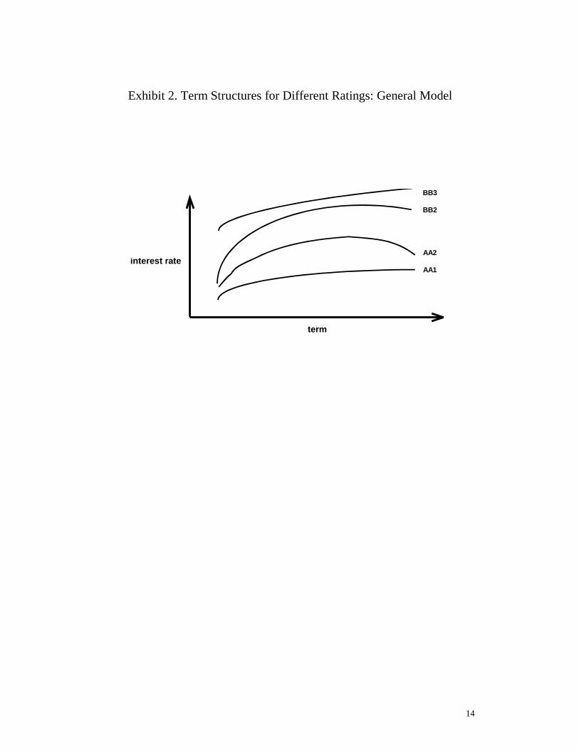
It is possible to exhibit more general models than that given in )4( (that is, a

model which allows the term structures obtained for different credit ratings to differ

not only by a translation factor). Exhibit 2 presents a schematic drawing of possibles

term structures of interest rates for different credit ratings, in a more general model.

3. Joint Estimation of Term Structures

Let us consider the simplest case first (that is, (4)). The objective is to estimate

the variables JiSi ,...,1, = and the coefficients ,...,, 321 ccc . The final results of this

estimation process are J different term structures of interest rates, each related to a

different rating.

Let us define the discount function )()( tD j for rating jr to be

( ) )5( ,...,1],,0[,)(exp)( )()( JjtttRtD jj =∈∀−= λ

We assume that m eurobonds are available to estimate the coefficients. We

assume that jm eurobonds possess a rating jr . The residual term ke of the statistical

fit obtained for the price of the thk eurobond satisfies

(6) ,...,2,1,)(111

)( mketDuooapk

k

f

lkkl

jkl

ccallk

pputkkk =∀+=−++

=

where kp denotes the price of the thk eurobond, ka denotes the accrued interest of

the thk eurobond, putk1 and call

k1 are dummy variables (Draper and Smith [1966])

6

indicating the existence of embedded put and call options in the eurobond, o p and oc

are unknown parameters related to the prices of the embedded put and call options,

kf denotes the number of remaining cash flows of the thk eurobond, klt the time

remaining for payment of the lth cash flow klu of the thk eurobond, and kj denotes

the rating of the thk eurobond (for instance, if the rating of the thk eurobond is 3r ,

then 3=kj ).

The estimation process is based in a two step procedure:

1. Identify influential observations (Rousseeuw and Leroy [1987]) using an

extension of Cook’s statistics (Atkinson [1988]). This first step is important

because in the Emerging Eurobond market there are many illiquid or “badly”

priced bonds. If these bonds are not appropriately handled during the estimation

phase, they may distort the term structures estimated.

2. Use a duration weighted estimation process after removing all the influential

observations detected in the first step. The estimation should preferably use robust

techniques, such as the Least Sum of Absolute Deviation or the Least Median of

Squares (Rousseeuw and Leroy [1987]). The use of duration weights incorporates

heteroskedasticity in the nonlinear regression model by allowing the volatility of

the eurobond prices to be proportional to its duration (as suggested in Vasicek and

Fong [1982]).

A numerical example illustrating the practical use of this methodology is

presented next.

4. A Numerical Example of the Estimation Process

Let us consider the joint estimation of Brazilian and Mexican eurobonds

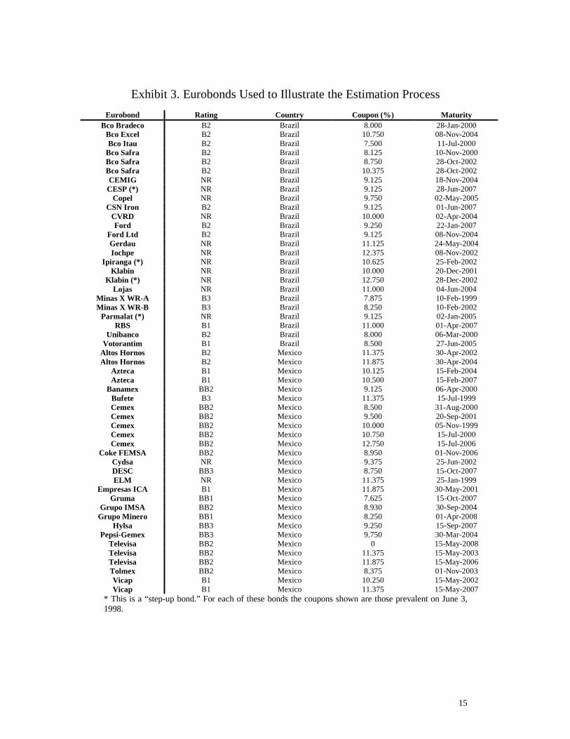
term structures using (4). Fifty-two eurobonds are used: twenty-five Brazilian;

twenty-seven Mexican. The eurobonds are classified in seven different credit ratings

(by Bloomberg Agency): BB1, BB2, BB3, B1, B2, B3 and NR (Not Rated). Exhibit 3

presents the main characteristics of the fifty-two eurobonds. Prices were collected on

June 3, 1998.

7

Three leverage points were detected in the first step of the estimation

process: one Brazilian (Iochpe); two Mexican (Bufete and Grupo Minero). Exhibit

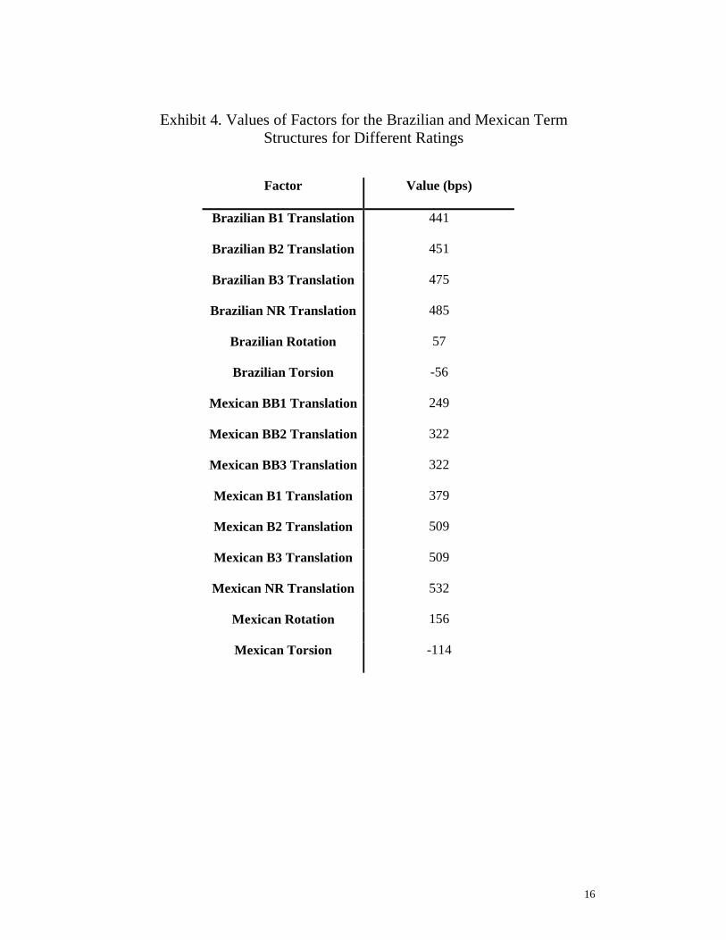
4 presents the parameters estimated for both the Brazilian and the Mexican eurobond

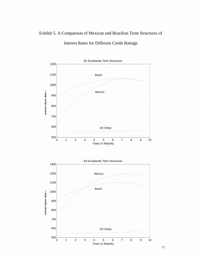
term structures. Exhibit 5 displays four estimated term structures: two related to the

credit rating B1; two related to the credit rating B3.

Note that for the Brazilian term structures, the translation factor varies just a

few basis points when different ratings are compared: for instance, the difference

between the B1 and the B3 translation factors is only 34 basis points (= 475 – 441; in

Exhibit 4). On the other hand there is a difference of 130 basis points between the B1

and B3 Mexican translation factors (= 509 – 379). This is a first indication that those

Brazilian companies (in Exhibit 3) issuing eurobonds presented more homogeneous

price values than the price of Mexican companies.

The next sections illustrate how the term structures in Exhibit 5 can be used

to exploit arbitrage in the Emerging Eurobond market. 5. Detection and Exploitation of Arbitrage Opportunities

The following five steps are proposed to detect and exploit arbitrage

opportunities in Latin American Eurobond markets:

1. Choose a set of eurobonds with a common rating.

2. Estimate the term structures of interest rates for each country.

3. Based on the estimated term structures, consider possible future scenarios for their

relative movement.

4. Analyze the sensitivity of different eurobond portfolios to the scenarios generated.

5. Obtain a portfolio that better adjusts to the scenarios expected.

Two numerical examples are presented to illustrate the practical use of these

five steps. These examples consider the following data4:

1. Brazil and Mexico: B1 Eurobonds.

2. Argentina and Mexico: BB2 Eurobonds.

8

5.1 Brazil and Mexico: B1 Eurobonds

Exhibit 5 depicts the Brazilian and the Mexican B1 term structures. The

Mexican term structure lies below the Brazilian term structure, indicating that the

Brazilian B1 eurobonds are “cheaper” when compared to Mexican B1 eurobonds.

The large difference between the translation, rotation and torsion factors of the

two term structures (see Exhibit 4) suggests as a probable future scenario one where

the curves converge to each other. That is, if there are no economic conditions leading

these two countries to behave radically different, we could expect their term

structures (with the same rating) to converge.

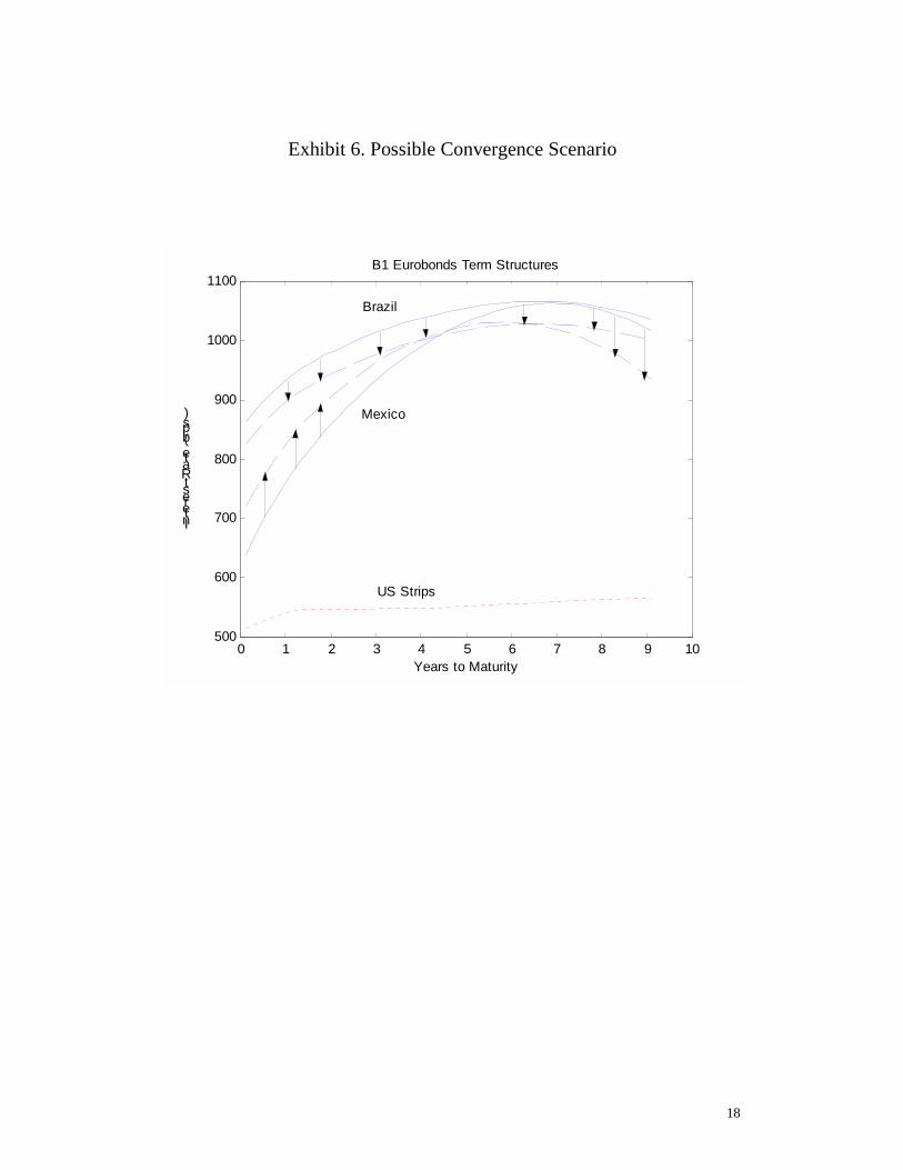
Exhibit 6 depicts a scenario for the convergence of the two term structures.

The arrows indicate the direction of the movements that would be observed for each

term structure in this situation. These scenarios could be associated with a decrease in

the external long term emerging markets borrowing rate. For the sake of illustration,

we consider as possible future scenarios only those where the Brazilian translation

factor and the Mexican rotation factor change their values.

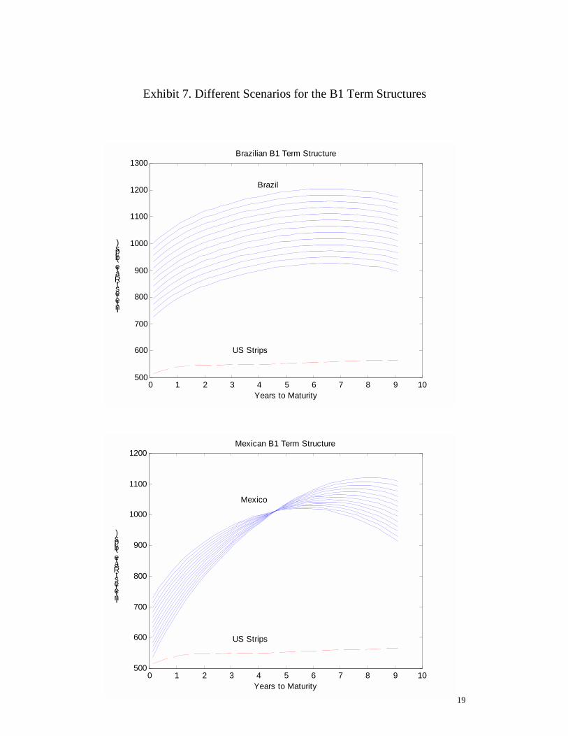
A set of scenarios for each term structure is generated. The prices of the

eurobonds for each of these scenarios are calculated. Exhibit 7 depicts possible

scenarios for the Brazilian and the Mexican term structures. Exhibit 8 presents the

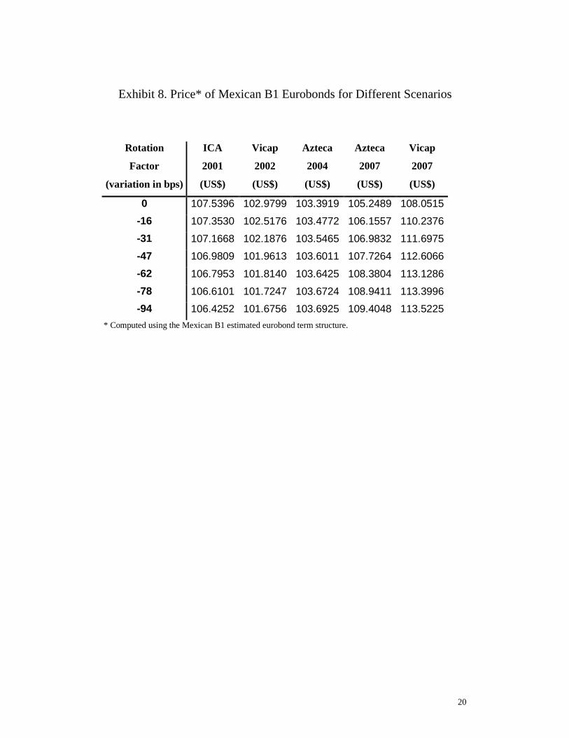
prices of the Mexican B1 eurobonds for six scenarios. Exhibit 9 presents the prices of

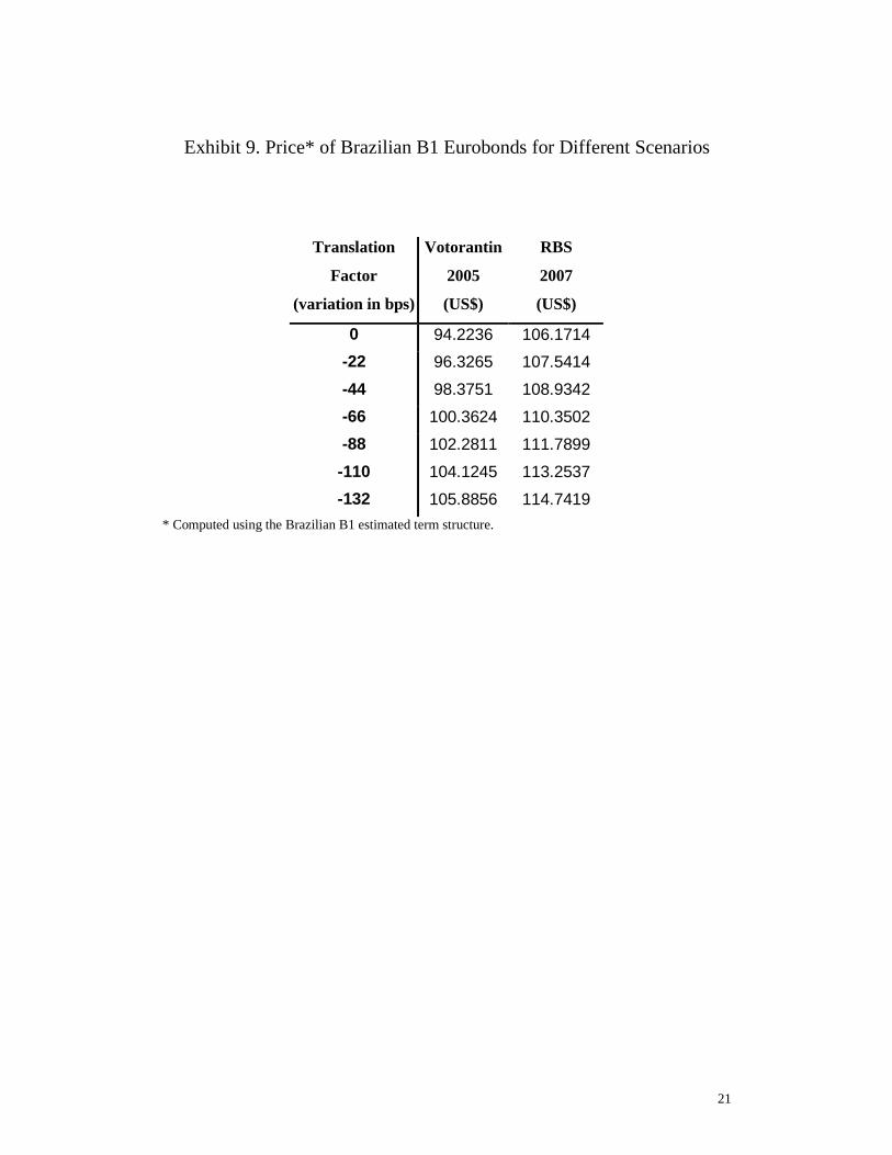
the Brazilian B1 eurobonds for six scenarios.

We note that a nine-year maturity is the largest in the Brazilian and Mexican

B1 eurobond market. We concentrate our analyses of the term structures in two

regions: region I, with maturities less than 4.5 years; and region II, with maturities

greater than 4.5 years. Exhibit 8 and Exhibit 9 show that in this situation, all Brazilian

B1 bonds would increase their values, short-term Mexican bonds (maturing in region

I; ICA 2001 and Vicap 2002) would decrease their values, and long-term Mexican

bonds (maturing in region II; Azteca 2004, Azteca 2007 and Vicap 2007) would

increase their values. A good strategy would be to buy Brazilian bonds and long-term

Mexican bonds, and to sell short-term Mexican bonds.

9

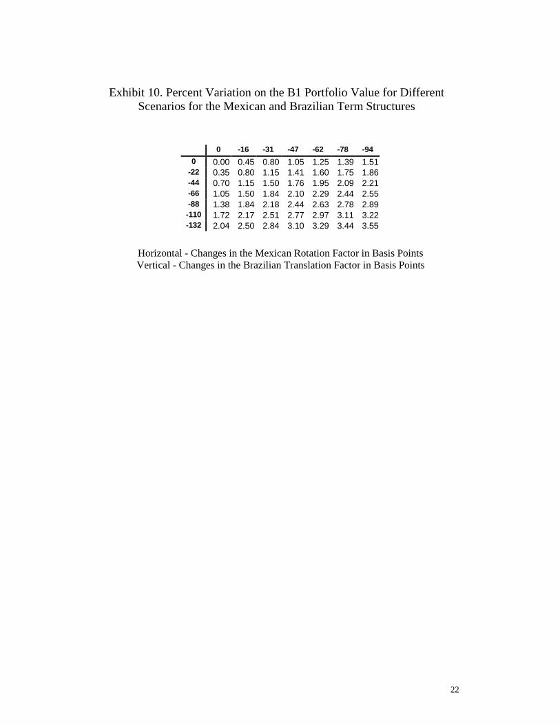
Exhibit 10 presents the percent variation of a proposed portfolio long Azteca

2004, Azteca 2007, Vicap 2007, Votorantin 2005 and RBS 2007, US$ 10 million

each, and short ICA 2001 and Vicap 2002, US$ 25 million each. In the most

favorable scenario the Mexican rotation factor decreasing by 94 basis points and

the Brazilian translation factor decreasing by 132 basis points the portfolio

provides a gain of 3.55%.

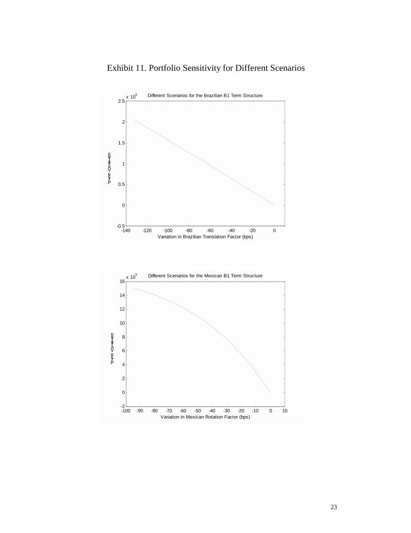
Exhibit 11 presents the portfolio sensitivity to the Brazilian translation factor

and the Mexican rotation factor. The plots in Exhibit 11 are interesting decision

making tools, providing an order of magnitude of possible gains/losses. Obviously,

the use of detailed risk management reports are strongly recommended to better

analyze the market risks involved in case the expected scenarios (in Exhibit 7) do not

materialize.

5.2 Argentina and Mexico: BB2 Eurobonds

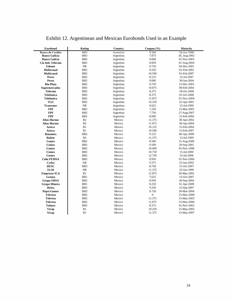
In this second example we consider the Argentinean and Mexican eurobond

markets. The eurobonds used for the joint estimation of term structures are given in

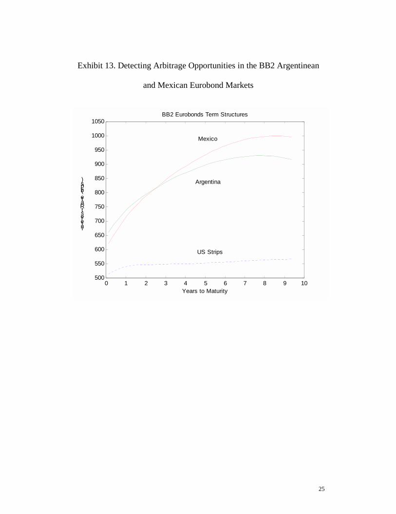
Exhibit 12. An example of the term structures estimated is given in Exhibit 13:

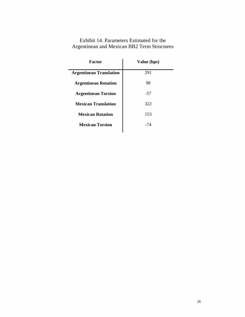
Argentinean and Mexican BB2 term structures. The parameters estimated for the two

BB2 term structures are given in Exhibit 14.

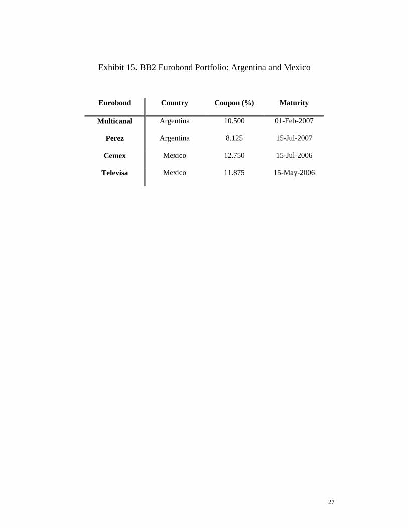
Let us suppose that a fixed income manager is positioned on a portfolio

composed by the eurobonds listed in Exhibit 15. Suppose as a probable scenario in

the near future is for a substantial reduction on long-term Mexican BB2 rates, a small

increase on short-term Mexican BB2 rates, and also a substantial reduction on

Argentinean BB2 rates. This scenario can be obtained by decreasing the Argentinean

translation factor to get the effect of reducing Argentinean interest rates, and a

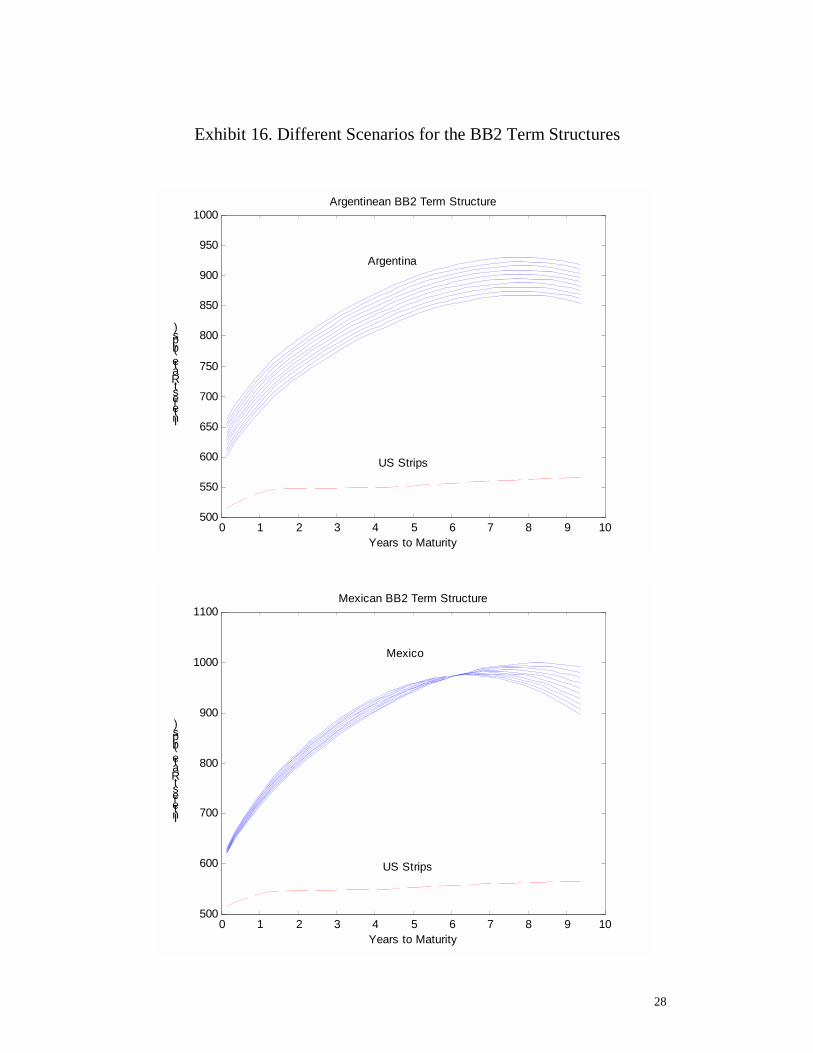
combination of changes in the Mexican rotation and torsion factors. Exhibit 16

depicts several scenarios incorporating these expectations. For example, in the most

extreme scenario considered, the Mexican term structure experiences a reduction of

approximately 90 basis points on long-term rates, an increase around 30 basis points

10

on medium-term rates, and an increase around 10 basis points on the short-term

interest rates.

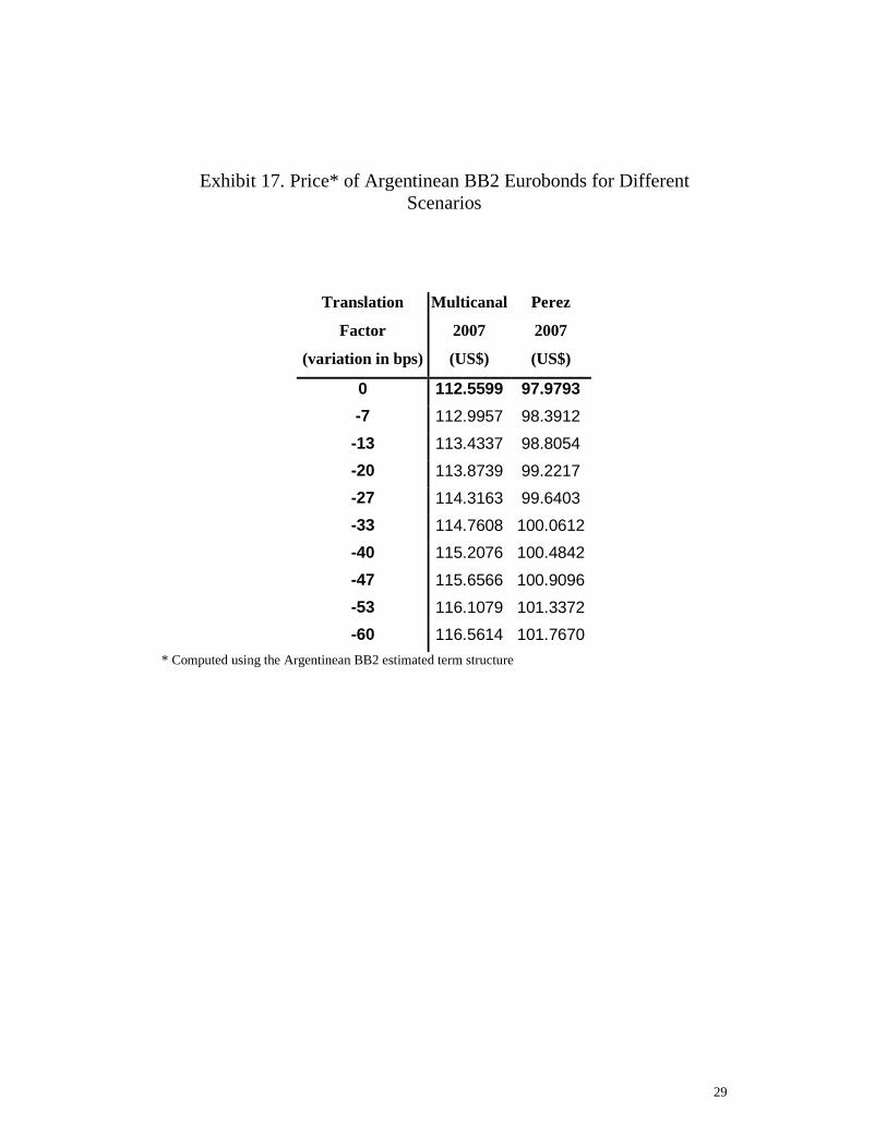
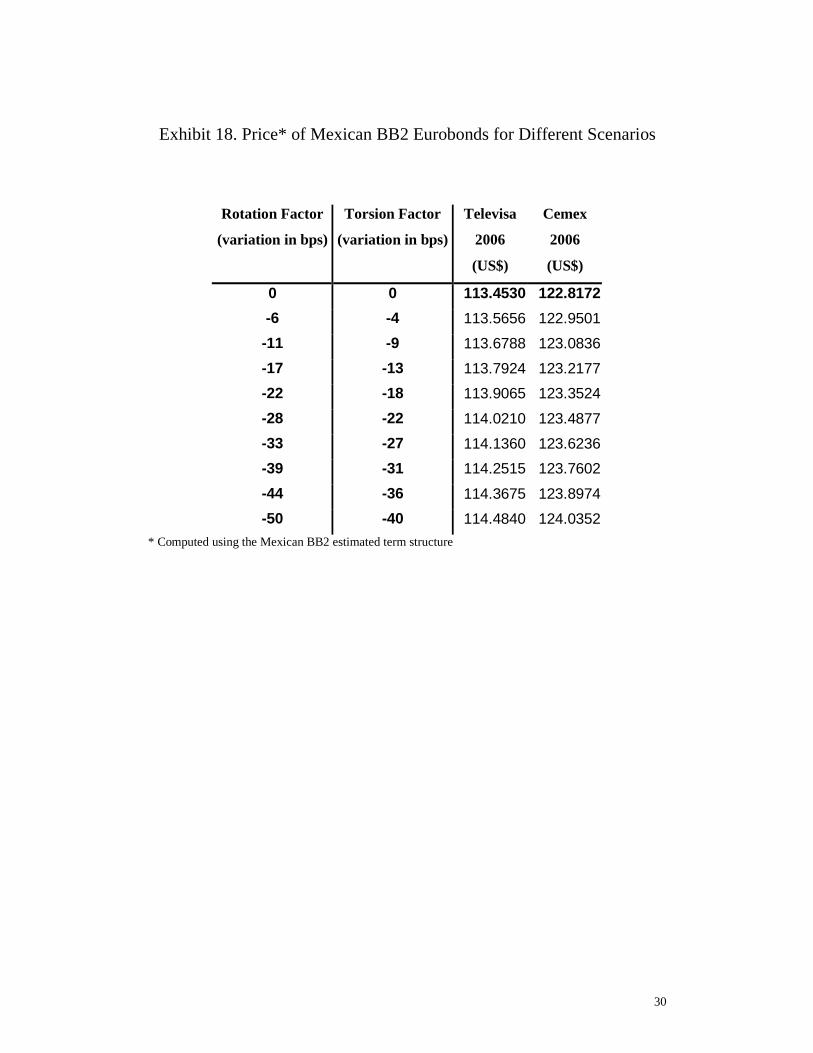
Exhibit 17 presents the prices for the Argentinean eurobonds in the manager’s

portfolio for nine scenarios. Exhibit 18 presents the prices for the Mexican eurobonds

for nine scenarios. The manager’s portfolio is composed by a long position in

Multicanal 2007, Perez 2007 and Televisa 2006, US$ 5 million, and a short position

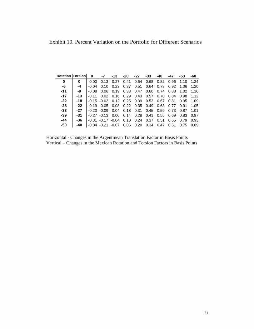
Cemex 2006, US$ 15 million. Exhibit 19 presents the portfolio percent variation for

each scenario depicted in Exhibit 16. We observe that the best performance of the

portfolio (for the scenarios displayed in Exhibit 19) provides a gain of 1.24%.

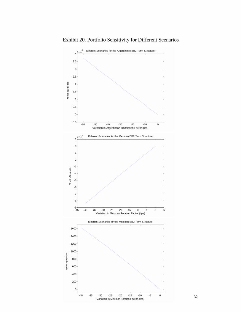
Finally, Exhibit 20 depicts the portfolio sensitivity to parallel changes in the

Argentinean term structure, and the rotational and torsional changes in the Mexican

term structures.

6. Conclusion

This article presents a methodology for the joint estimation of term structures

of interest rates of bonds with different credit ratings. The model is based on an

optimization procedure which assumes that the term structures movements are driven

by orthogonal factors. The estimated curves are useful for risk analysis, derivatives

pricing and portfolio selection. The methodology is efficient from the computational

point of view and is particularly useful when analyzing markets with few liquid

bonds, such as Emerging Eurobond markets. The methodology is completely

compatible with scenario analysis models for portfolio optimization and asset-liability

management.

Latin America Eurobond markets are used to illustrate the practical use of the

methodology. We explore some simple examples of arbitrage between international

term structures with the same rating, using scenario analysis to select portfolios.

Although the joint estimations realized in the article involve just pairs of countries

(Brazil versus Mexico and Argentina versus Mexico) the joint estimation process

could involve several countries.

11

References

Almeida, C.I.R., A.M.Duarte Jr. and C.A.C.Fernandes. “Decomposing and

Simulating the Movements of Term Structures of Interest Rates in Emerging

Eurobonds Markets”, Journal of Fixed Income, 1 (1998), pp. 21-31.

Atkinson, A.C. Plots, Transformations and Regression. Oxford: Oxford

Science Publications, 1988.

Black, F., E.Derman, and W.Toy. “A One-Factor Model of Interest Rates and

its application to Treasure Bond Options”, Financial Analysts Journal, 46 (1990), pp.

33-39.

Cox, J.C., J.E.Ingersoll, and S.A.Ross. “A Theory of the Term Structure of

Interest Rates”, Econometrica, 53 (1985), pp. 385-407.

Draper,N., and H.Smith. Applied Regression Analysis. New York: Wiley,

1966.

Heath, D., R.Jarrow, and A.Morton, “Bond Pricing and the Term Structure of

Interest Rates”, Econometrica, 60 (1992), pp. 77-105.

Ho, T.S.Y., and S.B.Lee, “Term Structure Movements and the Pricing of

Interest Rate Contingent Claims”, Journal of Financial and Quantitative Analysis, 41

(1986), pp. 1011-1029.

Hull, J., and A.White, “Numerical Procedures for Implementing Term

Structure Models I: Single Factor Models”, Journal of Derivatives, 2 (1994), pp. 7-

16.

Legendre, A.M. Sur l'Attraction des Sphéroides. Mémoires Mathematiques et

Physiques Présentés à l'Acadamie Royal Des Sciences, X, 1785.

Litterman, R. and T.Iben “Corporate Bond Valuation and the Term Structure

of Credit Spreads”, Technical Report, Financial Strategies Series, Goldman Sacks,

November 1988.

Litterman, R. and J.A. Scheinkman. “Common Factors Affecting Bond

Returns.” Journal of Fixed Income, 1 (1991), pp. 54-61.

Rousseeuw,P.J., and A.M.Leroy. Robust Regression and Outlier Detection.

New York: Wiley, 1987.

12

Sansone, G. Orthogonal Functions. New York: Interscience Publishers, 1959.

Singh, M.K. “Value-at-Risk Using Principal Components Analysis.” Journal

of Portfolio Management, 24 (1997), pp. 101-112.

Vasicek, O.A., and H.G.Fong. “Term Structure Modeling Using Exponential

Splines.” Journal of Finance, 37 (1982), pp. 339-348.

Vasicek, O.A. “An equilibrium Characterization of the Term Structure”

Journal of Financial Economics, 5 (1977), pp. 177-188.

13

Exhibit 1. Term Structures for Different Ratings: Simple Model

BB3

BB2

AA2interest rate

AA1

term

14

Exhibit 2. Term Structures for Different Ratings: General Model

BB3

BB2

AA2interest rate

AA1

term

15

Exhibit 3. Eurobonds Used to Illustrate the Estimation Process

Eurobond Rating Country Coupon (%) Maturity Bco Bradeco B2 Brazil 8.000 28-Jan-2000

Bco Excel B2 Brazil 10.750 08-Nov-2004 Bco Itau B2 Brazil 7.500 11-Jul-2000

Bco Safra B2 Brazil 8.125 10-Nov-2000 Bco Safra B2 Brazil 8.750 28-Oct-2002 Bco Safra B2 Brazil 10.375 28-Oct-2002 CEMIG NR Brazil 9.125 18-Nov-2004 CESP (*) NR Brazil 9.125 28-Jun-2007

Copel NR Brazil 9.750 02-May-2005 CSN Iron B2 Brazil 9.125 01-Jun-2007

CVRD NR Brazil 10.000 02-Apr-2004 Ford B2 Brazil 9.250 22-Jan-2007

Ford Ltd B2 Brazil 9.125 08-Nov-2004 Gerdau NR Brazil 11.125 24-May-2004 Iochpe NR Brazil 12.375 08-Nov-2002

Ipiranga (*) NR Brazil 10.625 25-Feb-2002 Klabin NR Brazil 10.000 20-Dec-2001

Klabin (*) NR Brazil 12.750 28-Dec-2002 Lojas NR Brazil 11.000 04-Jun-2004

Minas X WR-A B3 Brazil 7.875 10-Feb-1999 Minas X WR-B B3 Brazil 8.250 10-Feb-2002

Parmalat (*) NR Brazil 9.125 02-Jan-2005 RBS B1 Brazil 11.000 01-Apr-2007

Unibanco B2 Brazil 8.000 06-Mar-2000 Votorantim B1 Brazil 8.500 27-Jun-2005

Altos Hornos B2 Mexico 11.375 30-Apr-2002 Altos Hornos B2 Mexico 11.875 30-Apr-2004

Azteca B1 Mexico 10.125 15-Feb-2004 Azteca B1 Mexico 10.500 15-Feb-2007

Banamex BB2 Mexico 9.125 06-Apr-2000 Bufete B3 Mexico 11.375 15-Jul-1999 Cemex BB2 Mexico 8.500 31-Aug-2000 Cemex BB2 Mexico 9.500 20-Sep-2001 Cemex BB2 Mexico 10.000 05-Nov-1999 Cemex BB2 Mexico 10.750 15-Jul-2000 Cemex BB2 Mexico 12.750 15-Jul-2006

Coke FEMSA BB2 Mexico 8.950 01-Nov-2006 Cydsa NR Mexico 9.375 25-Jun-2002 DESC BB3 Mexico 8.750 15-Oct-2007 ELM NR Mexico 11.375 25-Jan-1999

Empresas ICA B1 Mexico 11.875 30-May-2001 Gruma BB1 Mexico 7.625 15-Oct-2007

Grupo IMSA BB2 Mexico 8.930 30-Sep-2004 Grupo Minero BB1 Mexico 8.250 01-Apr-2008

Hylsa BB3 Mexico 9.250 15-Sep-2007 Pepsi-Gemex BB3 Mexico 9.750 30-Mar-2004

Televisa BB2 Mexico 0 15-May-2008 Televisa BB2 Mexico 11.375 15-May-2003 Televisa BB2 Mexico 11.875 15-May-2006 Tolmex BB2 Mexico 8.375 01-Nov-2003 Vicap B1 Mexico 10.250 15-May-2002 Vicap B1 Mexico 11.375 15-May-2007

* This is a “step-up bond.” For each of these bonds the coupons shown are those prevalent on June 3, 1998.

16

Exhibit 4. Values of Factors for the Brazilian and Mexican Term Structures for Different Ratings

Factor Value (bps)

Brazilian B1 Translation 441

Brazilian B2 Translation 451

Brazilian B3 Translation 475

Brazilian NR Translation 485

Brazilian Rotation 57

Brazilian Torsion -56

Mexican BB1 Translation 249

Mexican BB2 Translation 322

Mexican BB3 Translation 322

Mexican B1 Translation 379

Mexican B2 Translation 509

Mexican B3 Translation 509

Mexican NR Translation 532

Mexican Rotation 156

Mexican Torsion -114

17

Exhibit 5. A Comparison of Mexican and Brazilian Term Structures of

Interest Rates for Different Credit Ratings

0 1 2 3 4 5 6 7 8 9 10500

600

700

800

900

1000

1100

1200

Years to Maturity

Interest Rate (bps)

B1 Eurobonds Term Structures

US Strips

Brazil

Mexico

0 1 2 3 4 5 6 7 8 9 10500

600

700

800

900

1000

1100

1200

1300

Years to Maturity

Interest Rate (bps)

B3 Eurobonds Term Structures

US Strips

Mexico

Brazil

18

Exhibit 6. Possible Convergence Scenario

0 1 2 3 4 5 6 7 8 9 10500

600

700

800

900

1000

1100

Years to Maturity

Interest Rate (bps)

B1 Eurobonds Term Structures

Brazil

Mexico

US Strips

19

Exhibit 7. Different Scenarios for the B1 Term Structures

0 1 2 3 4 5 6 7 8 9 10500

600

700

800

900

1000

1100

1200

1300

Years to Maturity

Interest Rate (bps)

Brazilian B1 Term Structure

US Strips

Brazil

0 1 2 3 4 5 6 7 8 9 10500

600

700

800

900

1000

1100

1200

Years to Maturity

Interest Rate (bps)

Mexican B1 Term Structure

US Strips

Mexico

20

Exhibit 8. Price* of Mexican B1 Eurobonds for Different Scenarios

Rotation

Factor

(variation in bps)

ICA

2001

(US$)

Vicap

2002

(US$)

Azteca

2004

(US$)

Azteca

2007

(US$)

Vicap

2007

(US$)

0 107.5396 102.9799 103.3919 105.2489 108.0515 -16 107.3530 102.5176 103.4772 106.1557 110.2376 -31 107.1668 102.1876 103.5465 106.9832 111.6975 -47 106.9809 101.9613 103.6011 107.7264 112.6066 -62 106.7953 101.8140 103.6425 108.3804 113.1286 -78 106.6101 101.7247 103.6724 108.9411 113.3996 -94 106.4252 101.6756 103.6925 109.4048 113.5225

* Computed using the Mexican B1 estimated eurobond term structure.

21

Exhibit 9. Price* of Brazilian B1 Eurobonds for Different Scenarios

Translation

Factor

(variation in bps)

Votorantin

2005

(US$)

RBS

2007

(US$)

0 94.2236 106.1714 -22 96.3265 107.5414 -44 98.3751 108.9342 -66 100.3624 110.3502 -88 102.2811 111.7899

-110 104.1245 113.2537 -132 105.8856 114.7419

* Computed using the Brazilian B1 estimated term structure.

22

Exhibit 10. Percent Variation on the B1 Portfolio Value for Different Scenarios for the Mexican and Brazilian Term Structures

0 -16 -31 -47 -62 -78 -94 0 0.00 0.45 0.80 1.05 1.25 1.39 1.51

-22 0.35 0.80 1.15 1.41 1.60 1.75 1.86-44 0.70 1.15 1.50 1.76 1.95 2.09 2.21-66 1.05 1.50 1.84 2.10 2.29 2.44 2.55-88 1.38 1.84 2.18 2.44 2.63 2.78 2.89

-110 1.72 2.17 2.51 2.77 2.97 3.11 3.22-132 2.04 2.50 2.84 3.10 3.29 3.44 3.55

Horizontal - Changes in the Mexican Rotation Factor in Basis Points Vertical - Changes in the Brazilian Translation Factor in Basis Points

23

Exhibit 11. Portfolio Sensitivity for Different Scenarios

-140 -120 -100 -80 -60 -40 -20 0-0.5

0

0.5

1

1.5

2

2.5x 106 Different Scenarios for the Brazilian B1 Term Structure

Price Variation

Variation in Brazilian Translation Factor (bps)

-100 -90 -80 -70 -60 -50 -40 -30 -20 -10 0 10-2

0

2

4

6

8

10

12

14

16x 105

Variation in Mexican Rotation Factor (bps)

Price Variation

Different Scenarios for the Mexican B1 Term Structure

24

Exhibit 12. Argentinean and Mexican Eurobonds Used in an Example

Eurobond Rating Country Coupon (%) Maturity Banco de Credito BB3 Argentina 9.500 24-Apr-2000

Banco Galicia BB3 Argentina 7.875 26_Aug-2002 Banco Galicia BB3 Argentina 9.000 01-Nov-2003

Cia Intl. Telecom BB2 Argentina 8.850 01-Aug-2004 Edenor NR Argentina 9.750 04-Dec-2001

Multicanal BB2 Argentina 9.250 01-Feb-2002 Multicanal BB2 Argentina 10.500 01-Feb-2007

Perez BB2 Argentina 8.125 15-Jul-2007 Perez BB2 Argentina 9.000 30-Jan-2004

Rio Plata BB2 Argentina 8.750 15-Dec-2003 Supermercados BB3 Argentina 10.875 09-Feb-2004

Telecom BB2 Argentina 8.375 18-Oct-2000 Telefonica BB3 Argentina 8.375 01-Oct-2000 Telefonica BB2 Argentina 11.875 01-Nov-2004

TGS BB2 Argentina 10.250 25-Apr-2001 Transener NR Argentina 9.625 15-Jul-1999

YPF BB2 Argentina 7.250 15-Mar-2003 YPF BB2 Argentina 7.750 27-Aug-2007 YPF BB2 Argentina 8.000 15-Feb-2004

Altos Hornos B2 Mexico 11.375 30-Apr-2002 Altos Hornos B2 Mexico 11.875 30-Apr-2004

Azteca B1 Mexico 10.125 15-Feb-2004 Azteca B1 Mexico 10.500 15-Feb-2007

Banamex BB2 Mexico 9.125 06-Apr-2000 Bufete B3 Mexico 11.375 15-Jul-1999 Cemex BB2 Mexico 8.500 31-Aug-2000 Cemex BB2 Mexico 9.500 20-Sep-2001 Cemex BB2 Mexico 10.000 05-Nov-1999 Cemex BB2 Mexico 10.750 15-Jul-2000 Cemex BB2 Mexico 12.750 15-Jul-2006

Coke FEMSA BB2 Mexico 8.950 01-Nov-2006 Cydsa NR Mexico 9.375 25-Jun-2002 DESC BB3 Mexico 8.750 15-Oct-2007 ELM NR Mexico 11.375 25-Jan-1999

Empresas ICA B1 Mexico 11.875 30-May-2001 Gruma BB1 Mexico 7.625 15-Oct-2007

Grupo IMSA BB2 Mexico 8.930 30-Sep-2004 Grupo Minero BB1 Mexico 8.250 01-Apr-2008

Hylsa BB3 Mexico 9.250 15-Sep-2007 Pepsi-Gemex BB3 Mexico 9.750 30-Mar-2004

Televisa BB2 Mexico 0 15-May-2008 Televisa BB2 Mexico 11.375 15-May-2003 Televisa BB2 Mexico 11.875 15-May-2006 Tolmex BB2 Mexico 8.375 01-Nov-2003 Vicap B1 Mexico 10.250 15-May-2002 Vicap B1 Mexico 11.375 15-May-2007

25

Exhibit 13. Detecting Arbitrage Opportunities in the BB2 Argentinean

and Mexican Eurobond Markets

0 1 2 3 4 5 6 7 8 9 10500

550

600

650

700

750

800

850

900

950

1000

1050

Years to Maturity

Interest Rate (bps)

BB2 Eurobonds Term Structures

US Strips

Argentina

Mexico

26

Exhibit 14. Parameters Estimated for the Argentinean and Mexican BB2 Term Structures

Factor Value (bps)

Argentinean Translation 291

Argentinean Rotation 98

Argentinean Torsion -57

Mexican Translation 322

Mexican Rotation 153

Mexican Torsion -74

27

Exhibit 15. BB2 Eurobond Portfolio: Argentina and Mexico

Eurobond Country Coupon (%) Maturity

Multicanal Argentina 10.500 01-Feb-2007

Perez Argentina 8.125 15-Jul-2007

Cemex Mexico 12.750 15-Jul-2006

Televisa Mexico 11.875 15-May-2006

28

Exhibit 16. Different Scenarios for the BB2 Term Structures

0 1 2 3 4 5 6 7 8 9 10500

550

600

650

700

750

800

850

900

950

1000

Years to Maturity

Interest Rate (bps)

Argentinean BB2 Term Structure

Argentina

US Strips

0 1 2 3 4 5 6 7 8 9 10500

600

700

800

900

1000

1100

Years to Maturity

Interest Rate (bps)

Mexican BB2 Term Structure

US Strips

Mexico

29

Exhibit 17. Price* of Argentinean BB2 Eurobonds for Different Scenarios

Translation

Factor

(variation in bps)

Multicanal

2007

(US$)

Perez

2007

(US$)

0 112.5599 97.9793 -7 112.9957 98.3912 -13 113.4337 98.8054 -20 113.8739 99.2217 -27 114.3163 99.6403 -33 114.7608 100.0612-40 115.2076 100.4842-47 115.6566 100.9096-53 116.1079 101.3372-60 116.5614 101.7670

* Computed using the Argentinean BB2 estimated term structure

30

Exhibit 18. Price* of Mexican BB2 Eurobonds for Different Scenarios

Rotation Factor

(variation in bps)

Torsion Factor

(variation in bps)

Televisa

2006

(US$)

Cemex

2006

(US$)

0 0 113.4530 122.8172 -6 -4 113.5656 122.9501 -11 -9 113.6788 123.0836 -17 -13 113.7924 123.2177 -22 -18 113.9065 123.3524 -28 -22 114.0210 123.4877 -33 -27 114.1360 123.6236 -39 -31 114.2515 123.7602 -44 -36 114.3675 123.8974 -50 -40 114.4840 124.0352

* Computed using the Mexican BB2 estimated term structure

31

Exhibit 19. Percent Variation on the Portfolio for Different Scenarios

Rotation Torsion 0 -7 -13 -20 -27 -33 -40 -47 -53 -60 0 0 0.00 0.13 0.27 0.41 0.54 0.68 0.82 0.96 1.10 1.24 -6 -4 -0.04 0.10 0.23 0.37 0.51 0.64 0.78 0.92 1.06 1.20

-11 -9 -0.08 0.06 0.19 0.33 0.47 0.60 0.74 0.88 1.02 1.16 -17 -13 -0.11 0.02 0.16 0.29 0.43 0.57 0.70 0.84 0.98 1.12 -22 -18 -0.15 -0.02 0.12 0.25 0.39 0.53 0.67 0.81 0.95 1.09 -28 -22 -0.19 -0.05 0.08 0.22 0.35 0.49 0.63 0.77 0.91 1.05 -33 -27 -0.23 -0.09 0.04 0.18 0.31 0.45 0.59 0.73 0.87 1.01 -39 -31 -0.27 -0.13 0.00 0.14 0.28 0.41 0.55 0.69 0.83 0.97 -44 -36 -0.31 -0.17 -0.04 0.10 0.24 0.37 0.51 0.65 0.79 0.93 -50 -40 -0.34 -0.21 -0.07 0.06 0.20 0.34 0.47 0.61 0.75 0.89

Horizontal - Changes in the Argentinean Translation Factor in Basis Points Vertical – Changes in the Mexican Rotation and Torsion Factors in Basis Points

32

Exhibit 20. Portfolio Sensitivity for Different Scenarios

-45 -40 -35 -30 -25 -20 -15 -10 -5 0 5-9

-8

-7

-6

-5

-4

-3

-2

-1

0

1x 10

4

Price Variation

Variation in Mexican Rotation Factor (bps)

Different Scenarios for the Mexican BB2 Term Structure

-60 -50 -40 -30 -20 -10 0-0.5

0

0.5

1

1.5

2

2.5

3

3.5

4x 10

5 Different Scenarios for the Argentinean BB2 Term Structure

Variation in Argentinean Translation Factor (bps)

Price Variation

-40 -35 -30 -25 -20 -15 -10 -5 0

0

200

400

600

800

1000

1200

1400

1600

Price Variation

Variation in Mexican Torsion Factor (bps)

Different Scenarios for the Mexican BB2 Term Structure