Credit Derivatives and the Default Risk of Large Complex

Financial Institutions

Giovanni Calice, Christos Ioannidis, Julian Williams1,∗

Abstract

This paper addresses the impact of developments in the credit risk transfer market on theviability of a group of systemically important financial institutions. We propose a bank defaultrisk model, in the vein of the classic Merton-type, which utilizes a multi-equation framework tomodel forward-looking measures of market and credit risk using the credit default swap (CDS)index market as a measure of the global credit environment. In the first step, we establish theexistence of significant detrimental volatility spillovers from the CDS market to the banks’ equityprices, suggesting a credit shock propagation channel which results in serious deterioration of thevaluation of banks’ assets. In the second step, we show that substantial capital injections arerequired to restore the stability of the banking system to an acceptable level after shocks to theCDX and iTraxx indices. Our empirical evidence thus informs the relevant regulatory authoritieson the magnitude of banking systemic risk jointly posed by CDS markets.

Keywords: Distance to Default, Credit Derivatives, Credit Default Swap Index, FinancialStabilityJEL Classification: C32, G21, G33

∗Corresponding AuthorEmail addresses: g.calice@soton.ac.uk (Giovanni Calice), c.ioannidis@bath.ac.uk (Christos

Ioannidis), julian.williams@abdn.ac.uk (Julian Williams)1We would like to thank the participants in the 50th Annual Conference of the Italian Economic Associ-

ation (Rome), The Money and Finance Research Group (MoFiR) Conference on The Changing Geographyof Money, Banking and Finance in a Post-Crisis World (Ancona); the XVII Finance Forum of the SpanishFinance Association (Madrid), the 2010 Annual Meeting of the Midwest Finance Association (Las Ve-gas), the French Finance Association 2010 International Spring Meeting (Saint-Malo), the National Bankof Poland Conference on “Heterogeneous Nations and Globalized Financial Markets: New Challenges forCentral Banks” (Warsaw), the CEPS/ECMI Workshop on “European Capital Markets: Walking on ThinIce/ECMI AGM” (Brussels), the IJCB Spring Conference on “The Theory and Practice of Macro-PrudentialRegulation” (Madrid), the Fifth International Conference on “Central Banking, Regulation and Supervi-sion after the Financial Crisis” Finlawmetrics 2010 (Bocconi University, Milan), the 5th Annual Seminaron Banking, Financial Stability and Risk of the Banco Central do Brasil on “The Financial Crisis of 2008,Credit Markets and Effects on Developed and Emerging Economies” (Sao Paulo), the Norges Bank Finan-cial Stability Conference on ”Government Intervention and Moral Hazard in the Financial Sector” (Oslo),the Federal Reserve Bank of Cleveland Conference on ”Countercyclical Capital Requirements” (Cleveland),the 10th Annual FDIC-JFSR Bank Research Conference on ”Finance and Sustainable Growth” (Arlington)and seminar series at the Deutsche Bundesbank, Banque de France, Banca d’Italia, Swiss National Bank,

Preprint September 28, 2010

1. Introduction

In 2007-2008 the global financial system has undergone a period of unprecedented in-

stability. The difference, however, between past financial crises and that which appears

to have begun in earnest in August 2007 is the presence of the credit derivatives (CDs)

market. The transmission of credit risk via these types of instruments appears, according

to international financial regulators, to have amplified the global financial crisis by offering

a direct and unobstructed mechanism for channelling defaults among a variety of types of

financial institutions. Whilst the causes of this crisis are fairly well recognized, the mecha-

nism of transmission of shocks between CDs markets and the banking sector is not so well

understood from an empirical perspective. In fact, the academic and practitioner literature

have not yet reached firm conclusions on the financial stability implications of credit default

swaps (CDSs) instruments.

The turbulences experienced during the crisis on OTC derivatives markets have prompted

regulators to find solutions to enhance the smooth functioning of these markets. It is crystal

clear that in a context of inadequate underwriting practices in the US subprime mortgage

markets and excessive granting of loans by non regulated entities, financial innovation based

on CDs was at the heart of the financial crisis.

The objective of this paper is to shed some light on the mechanisms involved in banking

stability by studying the credit default swap (CDS) index market during the 2005-2010

period and exploring how negative shocks affected financial institutions as the subprime

crisis of 2007 unfolded and then evolved into the global financial crisis of 2008. To explore

this issue, we address empirically the relationship between CDS index markets and the

viability of systemically important financial institutions.

We use a contingent claims approach, which explicitly integrates forward looking market

information and recursive econometric techniques to track the evolution of default risk for

Swedish Central Bank, Bank of Portugal, Federal Reserve Bank of Atlanta, International Monetary Fund,Lancaster University, University of Reading and University of Leicester. We are also grateful to Hans Hvide,Tim Barmby, Michel Habib, Chris Martin, Stuart Hyde, Michele Fratianni, Henri Pages, Daniel Gros andDavid Lando who were helpful in improving the paper. Any errors are our own.

2

a sample of 16 large complex financial institutions (LCFIs). We adopt the classic distance

to default (henceforth D-to-D) to the pricing of corporate debt. The well known market

based credit risk model is the Merton (1974) model, which views a firm’s equity liability as

a call option on asset with exercise price equals its total debt liability. By backing out asset

values and volatilities from quoted stock prices and balance sheet information, the Merton

(1974) model is able to generate updates of firms’ default probabilities. Since one of the

most important determinant of CDS prices is the likelihood of the reference entity involves

in a credit event, and this likelihood is tightly linked to stock market valuation as indicated

in the Merton (1974) theoretical framework, it is natural to investigate empirically the link

between the stock market and CDS markets.

A priori, it is not clear whether and to what extent CDS indices and LCFIs equity values

are related. We are not aware of any studies analyzing this relationship either theoretically

or empirically. There is a considerable volume of literature that attempts to describe the

effect of CDS on asset prices. Most of this literature relates to the co-movement of the CDS

market, the bond market and the equity market. However, to our knowledge, the closest

precursor to our analysis is the research by Bystrom (2005, 2006) and Longstaff (2010).

Bystrom (2004) finds a linkage between equity prices, equity return volatilities and CDS

spreads throughout studying a set of data from the European iTraxx CDS indices and stock

indexes.

Longstaff (2010) finds that during the subprime crisis of 2007, the value of asset-backed

collateralized debt obligations (CDOs) (using the ABX index as proxy) had a strong pre-

diction power for stock market returns (using the S&P 500 and the S&P 500 financial

subindex as proxies). He demonstrates empirically that the ABX indices were signalling

critical information of market distress by as much as three weeks ahead and he finds strong

evidence supporting a contagion mechanism - from the ABS subprime market to other fi-

nancial markets - driven primarily by market premia and liquidity channels instead of the

correlated-information channel. Although his data is limited to the period between 2006

and 2008 and the results focus only on the subprime crisis of 2007, the study is a highly

valuable contribution as it sheds light on the potential correlation between the ABX index

3

market and other financial markets (in primis, the equity market for financial institutions).

Our paper makes three distinctive contributions. The first contribution is a new approach

to modelling banking fragility that explicitly incorporates the transmission of corporate

credit risk from the CDS index market. Our model thus contributes to the existing literature

on credit risk models and measures of systemic risk by exploring the intuition that CD premia

are univariate timely indicators of information pertinent to systemic risks. To the best of our

knowledge, this paper is the first to combine the D-to-D analytical prediction of individual

banking fragility with measures of CD markets instability. While applications of the D-to-D

methodology have so far mostly concentrated in the option pricing literature, we show that

the Merton approach can be applied to the area of CRT. Hence, we provide a readable

implementable empirical application to infer default probabilities and credit risk (or other

tail behavior) on individual LCFIs.

To this purpose, we utilize a multivariate ARCH model to forecast the future volatility

of banks assets conditioned on the co-evolution of banks equity and the CDs market. The

incorporation of uncertainty and asset volatility are important elements in risk analysis since

uncertain changes in future asset values relative to promised payments on debt obligations

ultimately drive default risk and credit spreads - important elements of credit risk analysis

and, further, systemic risk (IMF, 2009). The econometric framework allows testing for the

predictive contribution of developments in the CD market on the stability of the banking

sector as depicted by the D-to-D of major financial institutions.

The paper includes a section that sets out the possible links between the value of banks

equity and the CDS market. The basic idea is that as banks deliberately undertake risky

projects that embed counter party risk the value and volatility of the banks assets will

co-evolve with developments in CDS markets.

In the same section we outline the econometric methodology we employ for the calculation

of the probability of default for the 16 institutions in our sample. We have opted for

a mixture of MV-GARCH model and Monte Carlo simulations instead of a multivariate

stochastic volatility model. We believe that this is a rather robust approach as it allows

us to obtain the empirical distribution of volatilities, based on the dynamic structure given

4

by the MV-GARCH model, and subsequently compute the probability of default when the

actual volatility is not known but its frequency distribution can be computed. A full account

of the methodology is presented in the paper.

The impact of developments in the CD market on the asset volatility is captured by

the evolution of the corporate investment-grade CDS indices (CDX and the iTraxx). CDX

North-American is the brand-name for the family of CDS index products of a portfolio

consisting of 5-year default swaps, covering equal principal amounts of debt of each of 125

named North American investment-grade issuers. The iTraxx Europe index is composed of

the most liquid 125 CDSs’ referencing European investment grade and high yield corporate

credit instruments.

In addition, the study makes a second methodological contribution. Having established

a relationship between CDS indices and our measure of fragility for LCFIs we turn the

focus of our analysis to the problem of determining an institution’s potential regulatory

capital requirement. To this end, we again use the VAR framework to perform a forward-

looking stress test exercise to estimate capital surcharges based on a variety of asset volatility

scenarios. Essentially, we impute the required capital injections per institution, based on

the distribution of the volatility of their own assets, given a-priori maximum probability of

default that is set at 1%. We believe that this setting constitutes a useful predictive tool

that financial regulators may wish to employ to gauge the implications for the stability of

systemically important financial institutions given developments in CDs markets.

The analytical foundations of our stress test scenario exercise draw from the stress test-

ing literature-thus allowing the model to focus on credit risk-and from the structured fi-

nance literature-thus enabling the model to consider the systemic effects of CDS shocks. By

adopting a clear and thorough methodology based on severe scenarios, providing detailed

bank-by-bank results and deploying, where necessary, remedial actions to strengthen the

capital position of individual banks, the stress test exercise is an important contribution to

strengthening the resilience and robustness of the global banking system.

In the past regulators have focused on traditional lending risks that form the basis of

bank capital requirements. The stress test provides a more rounded assessment of the

5

amount of equity a bank needs in order to be considered well capitalised relative to the

risks it is running. Since the goal is to lessen the probability of tail-risk scenarios, following

this approach, the regulator would be able to identify the highest default risk probability

assigned to each institution over the cycle and base the capital surcharge on that asset

volatility scenario.

The third contribution is an empirical test of this framework for an important category

of financial institutions, the Large Complex Financial Institutions (LCFIs), which can be

regarded as representative of the global banking system. The degree to which individual

banking groups are large in the sense that they could be a source of systemic risk depends

on the extent to which they can be a conduit for diffusing idiosyncratic and systemic shocks

through a banking system. Broadly we can distinguish between two types of pure shocks

to a banking system systemic and idiosyn1cratic. The focus of attention of the authorities,

entrusted with the remit of financial stability, is the monitoring of the impact of shocks

affecting simultaneously all the banks in the system.

A common finding in the empirical literature is that the level of banks’ exposure to

systemic shocks tends to determine the extent and severity of a systemic crisis. However,

another source of systemic risk may originate from an individual bank through either its

bankruptcy or an inability to operate. The transmission channel of the idiosyncratic shock

can be direct, for example if the bank was to default on its interbank liabilities, or indirect,

whereby a bank’s default leads to serious liquidity problems in one or more of the financial

markets where it was involved.

As far we are able to determine, this is the first investigation to establish a relationship

between the CDX and the iTraxx CDS indices and the banking sector which supports the

consideration of a transmission mechanism in order to account for the potential of default

risk of several global LCFIs. We adopt a working definition of banking instability as an

episode in which there is a significant increase in cross-market linkages after a shock occurs

in the CDS market.

In early 2009, the US Fed conducted stress tests on its banking industry and found

that 10 lenders needed nearly $75bn of additional capital between them. This managed to

6

soothe the markets and helped US banking stocks rebound. The stress tests were designed

to ensure the 19 leading US banks have enough capital in general, and equity in particular,

comfortably to survive a deeper-than-expected recession. They were also intended to provide

more standardized information about bank asset portfolios. Recently, the European Union

has also conducted stress tests on banks accounting for about 65 per cent of the EU banking

sector.

This application can be useful for supervisory scenario stress testing when complemented

with models of the probability of default and loss given default. Scenarios stress tests

involving both US and European LCFIs could help establish the level of impairment to

assets and capital needs.

Our most important findings are threefold. First, we find that systemically important

financial institutions are exposed simultaneously to systematic CDs shocks. In practice, we

find that the sensitivity of default risk across the banking system is highly correlated with

both the CDX and the iTraxx indices markets and that this relationship is of positive sign.

Hence, direct links between financial institutions and the CDS index market matter. This is

evidence of some spillover effects from the CDS market after the onset of the crisis. Second,

our model allows us to quantify the required capital needs for each LCFI via the overall

price-discovery process in the two CDS indices markets. The main insight from our estimates

is that the US government re-capitalization programmes considerably underestimated the

necessary capital injections for the US LCFIs. A plausible explanation for this result is

that the specification of our model does do not reflect any explicit or implicit government

guarantees on the total debt liabilities of the institutions. Third, XXXXXXXX

All our results have several important implications both for the financial stability lit-

erature and for global banking regulators. The study offers an insight on the intricate

interrelationships between CDS markets developments and the individual and the systemic

stability dimensions of the international banking system. It helps to quantify the trans-

mission of shocks and their volatility to a specific metric of financial stability. Our model

specification can help policymakers monitor default-risk and the distance to specific capital

thresholds of individual financial institutions at a daily frequency by testing the extent of

7

co-movements between North American and European CDS market conditions in normal as

well as stressful periods.

This suggests that our approach can serve as an early warning system for supervisors

to pursue closer scrutiny of a bank’s risk profile, thereby prompting additional regulatory

capital and enhanced supervision to discourage practices that increase systemic risk. The

remainder of the paper is organized as follows. Section §(2) briefly reviews the related

literature. Section §(3) outlines the theoretical foundations of our approach. Section 4

introduces the D-to-D approach and sketches in some detail our stress testing framework.

Section §(4) describes the data. The results are presented in §(5) and Section §(6) concludes.

2. Related Literature

The recent and growing literature on financial innovation and financial stability is char-

acterized by a lack of consensus on the net effect of CRT on the financial system. Duffie

(2008) discusses the costs and benefits of CRT instruments for the efficiency and the stability

of the financial system. The argument is that if CRT leads to a more efficient use of lender

capital, then the cost of credit is lowered, presumably leading to general macroeconomic

benefits such as greater long-run economic growth. CRT could also raise the total amount

of credit risk in the financial system to inefficient levels, and this could lead to inefficient

economic activities by borrowers. Allen and Gale (2006) develop a model of banking and

insurance and show that, with complete markets and contracts, inter-sectoral transfers are

desirable. However, with incomplete markets and contracts, CRT can occur as the result of

regulatory arbitrage and this can increase systemic risk.

Using a model with banking and insurance sectors, Allen and Carletti (2006) document

that the transfer between the banking sector and the insurance sector can lead to damaging

contagion of systemic risk from the insurance to the banking sector as the CRT induces

insurance companies to hold the same assets as banks. If there is a crisis in the insurance

sector, insurance companies will have to sell these assets, forcing down the price, which

implies the possibility of contagion of systemic risk to the banking sector since banks use

these assets to hedge their idiosyncratic liquidity risk.

8

Morrison (2005) shows that a market for CDs can destroy the signalling role of bank

debt and lead to an overall reduction in welfare as a result. He suggests that disclosure

requirements for CDs can help offset this effect. Bystrom (2005) investigates the relationship

between the European iTraxx index market and the stock market. CDS spreads have a strong

tendency to widen when stock prices fall and vice versa. Stock price volatility is also found to

be significantly correlated with CDS spreads and the spreads are found to increase (decrease)

with increasing (decreasing) stock price volatilities. The other interesting finding in this

paper is the significant positive autocorrelation present in all the studied iTraxx indices.

Building upon a structural credit risk model (CreditGrades), Bystrom (2006) reinforces

this argument through a comparative evaluation of the theoretical and the observed market

prices of eight iTraxx sub-indices. The paper’s main insight is the significant autocorrelation

between theoretical and empirical CDS spreads changes. Hence, this finding proves to

be consistent with the hypothesis that the CDS market and the stock market are closely

interrelated.

Baur and Joossens (2006) demonstrate under which conditions loan securitization can

increase the systemic risks in the banking sector. They use a simple model to show how

securitization can reduce the individual banks’ economic capital requirements by transferring

risk to other market participants and demonstrate that stability risks do not decrease due

to asset securitization. As a result, systemic risk can increase and impact on the financial

system in two ways. First, if the risks are transferred to unregulated market participants

where there is less capital in the economy to cover these risks and second if the risks are

transferred to other banks, interbank linkages increase and therefore augment systemic risk.

A recent study by Hu and Black (2008) concludes that, thanks to the explosive growth in

CDs, debt-holders such as banks and hedge funds have often more to gain if companies

fail than if they survive. The study warns that the breakdown in the relationship between

creditors and debtors, which traditionally worked together to keep solvent companies out

of bankruptcy, lowers the system’s ability to deal with a significant downwar shift in the

availability of credit.

There is also little consensus on the relative importance of CDS and bond markets, and

9

even less consensus on the CDS-equity markets relation. At least part of the difficulty has

to do with measurement.

Zhu (2003) discusses the role of the CDS market in price discovery. Using a vector

autoregression (VAR) framework, he finds that in the short run the results are slightly

in favour of the hypothesis that the CDS market moves ahead of the bond market, thus

contributing more to price discovery. Similar to Zhu approach, Longstaff, Mithal and Neis

(2005) use a VAR model to examine the lead-lag relationship between CDS, equity and

bond markets. They find that both changes in CDS premiums and stock returns often lead

changes in corporate bond yields. In Jorion and Zhang (2006) investigation of the intra-

industry credit contagion effect in the CDS market and the stock market, the CDS market

is found to lead the stock market in capturing the contagion effect.

The traditional literature on the empirical applications of the Merton Model has long

recognized that the D-to-D measure can be an efficient analytical predictor of individual firm

fragility. A vast number of contributions have been developed, particularly in the banking

literature. Chan-Lau et al (2004) measure bank vulnerability in emerging markets using the

D-to-D. The indicator is estimated using equity prices and balance-sheet data for 38 banks

in 14 emerging market countries. They find that the D-to-D can predict a bank’s credit

deterioration up to nine months in advance and it may prove useful for supervisory core

purposes.

Berndt, Douglas, Duffie, Ferguson and Schronz (2004) examine the relationship between

CDS premiums and EDFs. Moodys KMV EDFs are conditional probabilities of default,

which are fitted non-parametrically from the historical default frequencies of other firms

that had the same estimated D-to-D as the targeted firm. The D-to-D is the number of

standard deviations of annual asset growth by which its current assets exceed a measure of

book liabilities. They found that there is a positive link between 5-year EDFs and 5-year

CDS premiums. However, the sample only includes North American companies from three

industries. The result therefore might not be representative of the whole market.

Gropp et al (2006) show that the D-to-D may be a particularly suitable way to measure

bank risk, avoiding problems of other measures, such as subordinated debt spreads. The au-

10

thors employ the Merton’s model of credit risk to derive equity-based indicators for banking

soundness for a sample of European banks. They find that the Merton style equity-based

indicator is efficient and unbiased as monitoring device. Furthermore, the equity-based in-

dicator is forward looking and can pre-warn of a crisis 12 to 18 months ahead of time. The

D-to-D is able to predict banks’ downgrades in developed and emerging market countries.

Lehar (2005) proposes a new method to measure and monitor banking systemic risk.

This author proposes an index, based on the Merton model, which tracks the probability

of observing a systemic crisis - defined as a given number of simultaneous bank defaults -

in the banking sector at a given point in time. The method proposed allows regulators to

keep track of the systemic risk within their banking sector on an ongoing basis. It allows

comparing the risk over time as well as between countries. For a sample of North American

and Japanese banks (at the time of the Asian crisis in 1997/98) the author finds evidence

of a dramatic increase in the probability of a simultaneous default of the Japanese banks

whilst this decreases over time for the North American banks.

3. Methodology

We divide our empirical analysis into three sections. In the first section §§(3.1), we

develop a theoretical framework for objective levels of default risk. In the second section

of our investigation, §§(3.2), we outline a generalized stochastic volatility model of bank

assets with multiple volatility instruments. Finally in the third section §§(3.3), we define

an econometric model using a vector autoregressive model with multivariate autoregressive

conditionally heteroskedastic disturbances (VAR-MV-GARCH) to determine the time evo-

lution of the joint volatilities of the equity and our benchamrk CDS indices. We also extend

this model to infer forward looking simulations of the joint evolution of the asset value pro-

cess and hence determine the additional contingent capital requirements for each individual

LCFI.

11

3.1. Objective Levels of Default Risk

Consider a policy objective setting the default risk probability, over some relative time

horizon T − t, defined as p∗, such that for any systemically important institution, pi,t > p∗,

imposed by a regulator. The probability of default at time t, for the ith institution, will

be conditioned on the imputed conditional annualized volatility, σA,t, and value of assets,

VA,t. For any given systemically important financial institution suffering from some form

of financial distress, with probability of default, pi,t, the difference in probability p∗ − pi,t,

under the assumption of conditional normality, will correspond to the difference between

the minimum D-to-D set by the regulators and the current imputed distance

δi,t = η (p∗)− η (pi,t) (1)

If δi,t < 0, then we define δi,t as the distance to distress, if δi,t > 0, then we define δi,t as the

distance to capital adequacy. Given δi,t > 0, the required capital injection to boost the value

of assets to a point whereby η (p∗) = η (pi,t), i.e. γi,t = VA (p∗) − VA (pi,t), is defined as the

capital shortfall.

Assuming that VE is the observed value of equity and VL is the observed value of liabilities

at time t, we can treat the capital requirement problem as a typical option pricing problem.

We first take the standard assumption that VE is equivalent to a European call option on

assets at time T , which we impose exogenously. Furthermore we treat the liabilities as being

fixed. The value of this call option will be dependent on the properties of the underlying

stochastic process driving the value of assets, with structural parameters θA and the current

value of these assets VA,t, with strike price VL,t.

VE,t = C (t, T, VA,t, VL,t, θA) (2)

The value of the call option will be proportional to the probability of default

p ∝ C (t, T, VA,t, VL,tθA) (3)

12

furthermore assuming that for a given stochastic process the terminal distribution of asset

values at T is given by,

P (VA,T ) = Γ (VA,T ; t, T, VA,t, θA) (4)

for a regulator the objective is to assess whether the probability that the value of assets at

T will be less than the policy objective, i.e.

VL,T∫0

Γ (VA,T ; t, T, VA,t, θA) ds > p∗ (5)

this terminal distribution will depend on the choice of stochastic process driving VA,t.

3.2. A Stochastic Volatility Model of Bank Assets

We motivate our proposed relationship between the fluctuations of the banks’ assets and

developments in the market for CDS by considering the development of the value of the

assets VA of a typical bank with assets and liabilities VL.

Liabilities are fixed and are of known value and liquidity. Assets are chosen from a

portfolio VA of risky underlying assets and hedging instruments such that VA(t) = α′S(t) +

β′H(t), where S(t) and H(t) are vectors of risky and hedging instruments, respectively. The

appropriate length vectors of dynamically re-balanced weights that ensure the hedging ratio

maintains a target level of volatility are denoted by α and β . We define two risk vectors.

The first vector is the chosen level of risk σVA to which a bank exposes itself in order to

generate potential excess return. The second risk vector is the level of completeness of the

hedging instruments. We consider this risk vector to be driven by k − 1 risk instruments

xi ∈ {x1, . . . , xk−1} which can be regarded as representing counterparty risk embedded into

the hedging contracts used to control the banks exposure to risky assets and may or may

not be observed. Combining the assets and the instruments in the second risk vector, we

define the k length vector y (t) =[VA (t) , x1 (t) , . . . , xk (t)

]′and the multivariate stochastic

differential equation that denotes its time evolution as follows

dy (t) = µ (y (t) |θ ) dt+ σ (y (t) |θ ) dW (t) (6)

13

where µ is a vector/matrix function of drifts, σ is a vector/matrix function driving volatility

and W (t) is a k dimensional Weiner process, i.e. W i (t+ h)−W i (t) ∼ N (0, h). Regarding

the the nature of µ(·) and σ(), we proceed following the approach suggested by Williams

and Ioannidis (2010) and adopt a stochastic covariance model of the form

dy (t) = r (y (t)) dt+ Σ12 (t) (idiag (y (t)) dW (t)) (7)

ΣA (t) = A (t)A′ (t) (8)

A (t) = ivech (log a (t)) (9)

da (t) = λ (a (t)) dt+ ξ (a (t)) dW (t)σ (10)

where r (y (t)) =[rVA (t) , µ1x1 (t) , . . . , µk−1xk−1 (t)

]′The first term indicates that the evo-

lution asset growth is based on the instantaneous risk free rate r and {µ1, . . . , µk−1} are

the independent drifts of the instruments. The stochastic covariance matrix ΣA (t) consists

of a 12k (k + 1) vector stochastic process a(t). For simplicity, we set λ, for the covariance

process to zero and the volatility of volatility function, ξ (·) , is considered time invariant

ai(t) ∈ R. Williams and Ioannidis (2010) derive the optimal number of hedging instruments

for a simple stochastic covariance model to be 12k (k + 1)+1, given k diagonal and 1

2k (k − 1)

off-diagonal processes driving the volatility component. The attractive feature of this model

is that it enables to derive an analytic specification of a single quantity that combines all

the relevant variance and covariance terms as ΣA (t) is guaranteed to be PSD. The evolution

of y(t) from time t to t + h can be represented by an instantaneous multivariate Brownian

motion with covariance matrix

ΣA (t, t+ h) =

t+h∫t

f (dW (t)σ)ds (11)

where f is a function that aggregates the steps in the volatility equation in 7. The use

of the ivech transformation ensures positive semi-definiteness (PSD) on any instantaneous

realization of Σt that allows for its factorization. Now, we denote Σ12 (t) as the matrix

14

square-root of the instantaneous covariance matrix Σ(t). Depending upon the complexity

of the assumed processes driving a we can find either an analytic solution to the variance

of volatility density or use Monte Carlo simulations. Here, we implement a Monte Carlo

estimation procedure. A European call option on the bank’s assets would therefore be priced

over the integral of the possible volatilities

C (t, T, VS, K |θ ) =

∞∫0

Φ (σs)C (t, T, Vs, K, σs) ds (12)

where K is the strike price, T is the maturity of the call, under the assumption of an

equivalent time horizon T − t = h. Next we assign the C to denote the individual Black

and Scholes price of a call option with volatility σs, over an experiment space with respect

to s. Note that we are unable to observe the continuous time asset process. However, the

specification of our model can predict values of the call option, i.e. the value of equity,

that exhibit some form of stochastic covariation with the evolution of the chosen volatility

instruments. Therefore, we incorporate this property into an econometric specification of

equity. Consequently, the actual realisation of the volatility of equity results from the matrix

squareroot of the instantaneous covariance between equity and CDS indices and not merely

from the squareroot of the realisation of its variance. In practice this means simulating

across the parameter space of Σ(t), to generate draws of the volatility process.

3.3. Econometric Specification

Under the framework illustrated above, we use a vector autoregression (VAR) model,

yt = Zyt−1 +µ+ut, with BEKK type multivariate autoregressive conditionally heteroskedas-

tic disturbances to define the discrete time dynamics of the mean and variance systems.

Z is the 3 × 3 matrix of lagged coefficients, µ is a vector of intercepts and ut is a dis-

turbance process with conditional covariance matrix Etutu′t = Σt. The vector of interest

is the VAR of the equity returns and log differences of the CDX and iTraxx CDS indices,

yt = [∆ log (VE,t) ,∆ log (CDXt) ,∆ log (iT raxxt)]′. The VAR model disturbances are driven

15

by a BEKK conditional covariance model

Σt = KK ′ + AΣt−1A′ +But−1ut−1B

′ (13)

We impose a lag order of one on both the mean and variance covariance equations. KK ′

is the intercept in the variance equation and A and B are the 3 × 3 ARCH and GARCH

autoregression coefficients, respectively. The long run covariance matrix of the VAR system

disturbances takes the following form

vecΣ = (I − A⊗ A−B ⊗B)−1 vec (KK ′) (14)

The structural disturbances εt are computed from Σ12t ut = εt, where Σ

12t is the matrix square

root of Σt. Note that the mean and variance models are jointly estimated with maximum like-

lihood estimation (MLE). Setting the parameter vector θ as θ = [vecZ ′, µ′, vechK ′, vecA′, vecB′]′,

the MLE objective function is given by

L(θ)

, max

(−1

23T log (2π) +

T∑t=1

`t |θ

)(15)

where the recursion of the likelihood function is

`t |θ = det logKK ′ + A′Σt−1A+B′ (yt−1 − Zyt−2 − µ) (yt−1 − Zyt−2 − µ)′B

+ (yt − Zyt−1 − µ)′ . . .

×(KK ′ + AΣt−1A

′ +B (yt−1 − Zyt−2 − µ) (yt−1 − Zyt−2 − µ)′B′)−1

. . .

× (yt − Zyt−1 − µ) (16)

Using the estimated VAR and MV-GARCH parameters, we generate a set of Monte Carlo

pathways to simulate a set of possible future asset volatilities and then stratify these into a

set of future volatility scenarios.

16

3.4. Forward Looking Simulations

Specifically, we draw N one year (252 days) pathways of the 3× 1 column vector εt, i.e.

for the s (yt+s, Σt+s

) ∣∣εt+(s−1), . . . , εt; θ (17)

For each pathway, we compute the annualized average volatility2. We use to represent

the draw and evolution from one sample path. Following Hwertz (2005) who demonstrated

that BEKK type processes exhibit time varying multivariate fourth moments, we conduct

our simulation study across these time paths to capture this effect. We then sum over one

forward looking year Σ =∑252

s=1 Σt+s

∣∣εt+(s−1), . . . , εt; θ. Using the methodology of Merton,

we then compute for each pathway the value of assets, the volatility of assets, the distance

to default and the average probability of default.(VA, σA, η, p

), ?? outlines our approach

to computing the Merton model for a deterministic volatility. We then weight each of these

pathways by 1N

and sort them via the pathway average asset volatility. We exclude the top

and bottom 2.5% of the simulated asset volatilities and stratify the rest into ten quantiles,

ordered from low to high volatility levels. For each of these volatility quantiles, σi∈1,...,10A , we

then derive the asset volatilities and compute the D-to-D for a variety of asset levels starting

with the current implied asset value VA,t. To obtain the current asset value we take a mean

of the asset values computed over the three trading months (66 days) prior to April 29, 2009.

To further implement our test, we then construct an upward sloping curve relating the extra

required assets ∆VA against the D-to-D, for the ith volatility quantile, η∗∣∣∣VA + ∆VA;σiA .

For a particular objective D-to-D we can then compute the increase in assets required to

reestablish adequate capital buffers for each bank.

4. Data Sample

The group of LCFIs consist of eight US based institutions, three UK banks, two French

banks, two Swiss and one German banks. The Bank of England Financial Stability Review

2The variance-covariance matrices over all the paths will be centred around Σ

17

(2001) [? ] sets out classification criteria for LCFIs. Marsh, Stevens and Hawkesby (2003) [?

] provide substantial empirical evidence for this classification. To join the group of LCFIs

studied, a financial institution must feature in at least two of six global rankings on a variety

of operational activities (these are set out in table 1). We base our classification on the

2003 rankings so that all the systemically important financial institutions prior to the recent

financial crisis are included. These institutions are systemically important as the fallout from

a bank failure can cause destabilizing effects for the world financial system. It is not only an

institution’s size that matters for its systemic importance - its interconnectedness and the

vulnerability of its business models to excess leverage or a risky funding structure matter as

well. These financial institutions are ABN Amro/Royal Bank of Scotland, Bank of America,

Barclays, BNP Paribas, Citigroup, Credit Suisse, Deutsche Bank, Goldman Sachs, HSBC

Holdings, JP Morgan, Lehman Brothers, Merrill Lynch, Morgan Stanley, Societe Generale

and UBS. In addition, we consider Bear Stearns, given its crucial role as market-maker in

the global CDs market.

The CDX and iTraxx CDS indices are broad investment-grade barometers of investment

grade risk and preliminary studies suggest that these offer a reasonable benchmark of the

corporate credit environment. The data used in this paper is presented in Table ??. The

sample period extends from October 20, 2003 to April 29, 2009 for a total of 1462 trading

days. All data is obtained from Thomson Reuters, Datastream. Liabilities are reported on

a quarterly basis and are interpolated to daily frequency using piecewise cubic splines. The

equity value of the LCFIs utilized in the VAR-MV-GARCH model are dividend adjusted.

The market capitalization values are computed from the product of the number of shares

(NOSH), the closing equity price (PC) and the index adjustment factor (AF), (Datastream

series types in parentheses).

Appendix ?? presents our methods of analysis of the indices available to measure credit

risk. Figures ?? to ?? illustrate the evolution of the variables used in the econometric model

over the sample period, in addition to several other CDS benchmarks that we have examined

in the data analysis stage of this research.

18

Table 1: LCFI Inclusion Criteria, Source: Marsh, Stephens and Hawkesby (2003), page 94

1. Ten largest equity bookrunners world-wide2. Ten largest bond bookrunners world-wide3. Ten largest syndicated loans bookrunners world-wide4. Ten largest interest rate derivatives outstanding world-wide5. Ten highest FX revenues world-wide6. Ten largest holders of custody assets world-wide.

Table 2: Data InformationShort Name Full Name DataStream Mnemonic Thomson-Reuters Code

BOA Bank of America U:BAC 923937BS Bear Stearns U:BSC 936911

CITI Citigroup U: C 741344GS Goldman Sachs U: GS 696738

JPM JP Morgan U: JPM 902242LB Lehman Brothers U: LEH 131508ML Merrill Lynch U: MER 922060MS Morgan Stanley U: MWD 327998SG Societe Generale F: SGE 755457

BNP BNP Paripas F: BNP 309449DB Deutsche Bank D: DBK 905076CS Credit Suisse S: CSGN 950701

UBS UBS S: UBSN 936458BARC Barclays BARC 901443HSBC HSBC HSBA 507534

RBS Royal Bank of Scotland RBS 901450

19

4.1. Causation in Mean and Variance

We set up two restriction tests for our econometric methodology. The first is a con-

ventional directional block exogeneity test to test for directional effects on bank equity

returns. We define Z = [zi] where zi is the ith row of the mean equation coefficients,

zi = [zi,1, zi,2, zi,3]. The system consistent restriction allows for correlation in the structural

disturbances ut, but not in the autoregressive terms, Therefore, the restricted regression is of

the form yt = (I ◦ Z) yt−1 +µ+ut, where I is a 3×3 identity matrix and ◦ is the Hadamard

or element by element product. Setting the evaluated log likelihood of the restricted regres-

sion to L∗(θ1)

versus the unrestricted regression L∗(θ)

, the standard likelihood ratio test

of the in mean restriction is Λ1 = 2(L∗(θ)− L∗

(θ1))

, where Λ1 ∼ χ2(6), for each of the

block restrictions.

The variance test is slightly more complex, since the restrictions are block cross products.

Again setting yt = Zyt−1 + µ+ ut, the BEKK restriction is of the form

Σt = 12

(KK ′ + AΣt−1A

′ + But−1ut−1B′)

(18)

where A = Ψ ◦ A, B = Ψ ◦B, K = Ψ ◦K, with block restriction

Ψ =

√

2 0 0

0 1 1

0 1 1

(19)

setting the restricted likelihood to be L∗(θ2)

versus the unrestricted regression L∗(θ)

. The

likelihood test statistic is Λ2 = 2(L∗(θ)− L∗

(θ2))

. In total 12 parameters are restricted.

Therefore, Λ2 ∼ χ2(12), under the assumption of asymptotic normality3.

3To see how the covariance restriction works note that 12ΨΨ′ =

1 0 00 1 10 1 1

20

4.2. Parameter Stability Tests

Out data sample covers the period October 20, 2003 to April 29, 2009 and hence fully

covers the financial crisis that began in August 2007. An important consideration in the

parameter estimation and inference testing for this type of model is the issue of structural

breaks and substantial time variation in the underlying true parameters. To account for

this, we utilize a rolling versus static parameter estimation, which is an adaptation of the

modified KLIC forecast breakdown approach suggested in Giacomini and Rossi (2010). We

specify a minimum rolling window size of 20% of the complete sample, which is l = 292 days.

We estimate the model using a rolling window starting at t − l, t, i.e. taking t = 292 as

the starting date (November 30, 2004). We now consider two models: the model estimated

ex-post over the whole sample, denoted with superscript W and the rolling model denoted

with the superscript R. Consequently, the rolling sample comparative log likelihoods are

LRt

(θRt

), max

(−1

23T log (2π) +

t∑t−l

`t∣∣θRt)

(20)

LWt

(θW)

, −123T log (2π) +

t∑t−l

`t∣∣θW (21)

The rolling Kullback-Leibler statistic is defined as κt = LRt

(θRt

)− LW

t

(θW)

. Setting ς to

be the heteroskedasticity and autocorrelation consistent estimate of the standard deviation

of κt, we construct the rolling sum λt =∑t

t=1 ς−1κt, for t ∈ {1, ..., T}. Diebold and Mariano

(1996) derive the limit theorem for this type of comparative forecast statistic under relatively

mild distributional assumptions, suggesting that λt ∼ N (0, 1), as T →∞. As a robustness

check, we construct a Monte Carlo simulation with random and persistent jumps. These

jumps are both positive and negative in magnitude. From the simulation we generate draws

of λt. The Kolomogorov-Smirnoff test failed to reject the null of equality for 10,000 draws

versus 10,000 draws from a N (0, 1) distribution.

21

4.3. Estimating The Forward Looking Recapitalization Requirements

We establish a policy forecast period of one year, beginning on April 29, 2009. To

compute the simulations suggested in §§(3.4), we need to discriminate between the parameter

vectors θ ∈ {θRT , θW}, i.e. the whole period vector and the last 292 day estimated rolling

window parameter vector. We use the whole sample model parameters θW as the benchmark

and only choose θRT if the rolling window coefficients pertain to a better fit over the majority

of the preceding 292 days. For instance, under the normality assumption this means that

λt < 1.96 for more than 147 days out of 292, from t = T −292 to t = T , where T is April 29,

2009. We repeat this exercise for each bank. We report the optimal forward looking model

in Tables .4 and .5. In practice, the rolling window is preferred in the case of all 16 banks

in the sample4.

For each set of optimal forward looking parameters, we compute the restriction tests,

described in §§(4.1). The results are presented in Table 3. Again, we can observe that for

every bank in the analysis we reject the inclusion of the block exogeniety restrictions in

mean and variance.

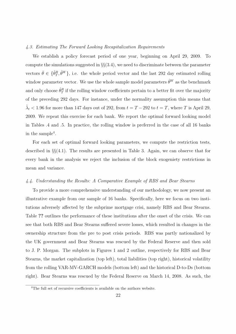
4.4. Understanding the Results: A Comparative Example of RBS and Bear Stearns

To provide a more comprehensive understanding of our methodology, we now present an

illustrative example from our sample of 16 banks. Specifically, here we focus on two insti-

tutions adversely affected by the subprime mortgage crisi, namely RBS and Bear Stearns.

Table ?? outlines the performance of these institutions after the onset of the crisis. We can

see that both RBS and Bear Stearns suffered severe losses, which resulted in changes in the

ownership structure from the pre to post crisis periods. RBS was partly nationalized by

the UK government and Bear Stearns was rescued by the Federal Reserve and then sold

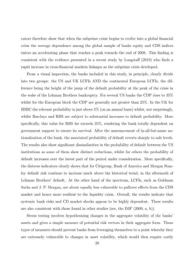
to J. P. Morgan. The subplots in Figures 1 and 2 outline, respectively for RBS and Bear

Stearns, the market capitalization (top left), total liabilities (top right), historical volatility

from the rolling VAR-MV-GARCH models (bottom left) and the historical D-to-Ds (bottom

right). Bear Stearns was rescued by the Federal Reserve on March 14, 2008. As such, the

4The full set of recursive coefficients is available on the authors website.

22

Table 3: The block exogeniety/causation tests in mean, Λ1, and variance Λ2 for each bank in the sample.

Λ1 p− value Λ2 p− valueBOA 186.3036 0.0000 4,210.4354 0.0000BS 5,000.4120 0.0000 12,936.3721 0.0000CITI 173.4772 0.0000 4,078.8147 0.0000GS 131.8649 0.0000 2,299.6358 0.0000JPM 216.0993 0.0000 3,110.2434 0.0000LB 133.2388 0.0000 5,205.7893 0.0000ML 1,410.7806 0.0000 4,754.0902 0.0000MS 213.7156 0.0000 3,130.9067 0.0000SG 156.1321 0.0000 2,328.5144 0.0000BNP 188.3487 0.0000 2,362.9616 0.0000DB 200.1796 0.0000 2,524.7460 0.0000CS 206.2118 0.0000 2,354.1980 0.0000UBS 190.0040 0.0000 2,567.1817 0.0000BARC 129.5412 0.0000 3,069.9669 0.0000HSBC 171.0778 0.0000 2,892.7295 0.0000RBS 121.8059 0.0000 3,794.0576 0.0000

we truncate the rolling analysis at this point. Consequently, we run the forward looking

recapitalization requirement from this date. Note that RBS stock was still traded until the

end of the sample window. Therefore, we carry the analysis forward to the truncation date,

that is April 29, 2009. Note also that, in addition to Bear Stearns, Merrill Lynch (acquired

by Bank of America) and Lehman Brothers (filed for bankruptcy on September 15, 2008)

are no longer traded as a separate entity within the sample.

We next compute the rolling parameter estimates for each model versus the whole sample

parameter estimates. We present four examples for each bank over the sample period. These

are plotted in Figures 3 and 4. We can observe the first order vector autoregressive coefficient,

z1,1 on equity (top left), the variance equation intercept coefficient on the equity, k1,1, (top

right), the lagged coefficient transmitting the lag of the CDX to equity, z1,2, (bottom left),

and finally the variance equation intercept cross product k1,2 for the variance of equity from

the lagged squared disturbance in the CDS index (top right).

Using the time varying parameters, we can compute the rolling comparative test statistic

and infer the correct forward looking model specification. Figures 5 and 6 present the rolling

23

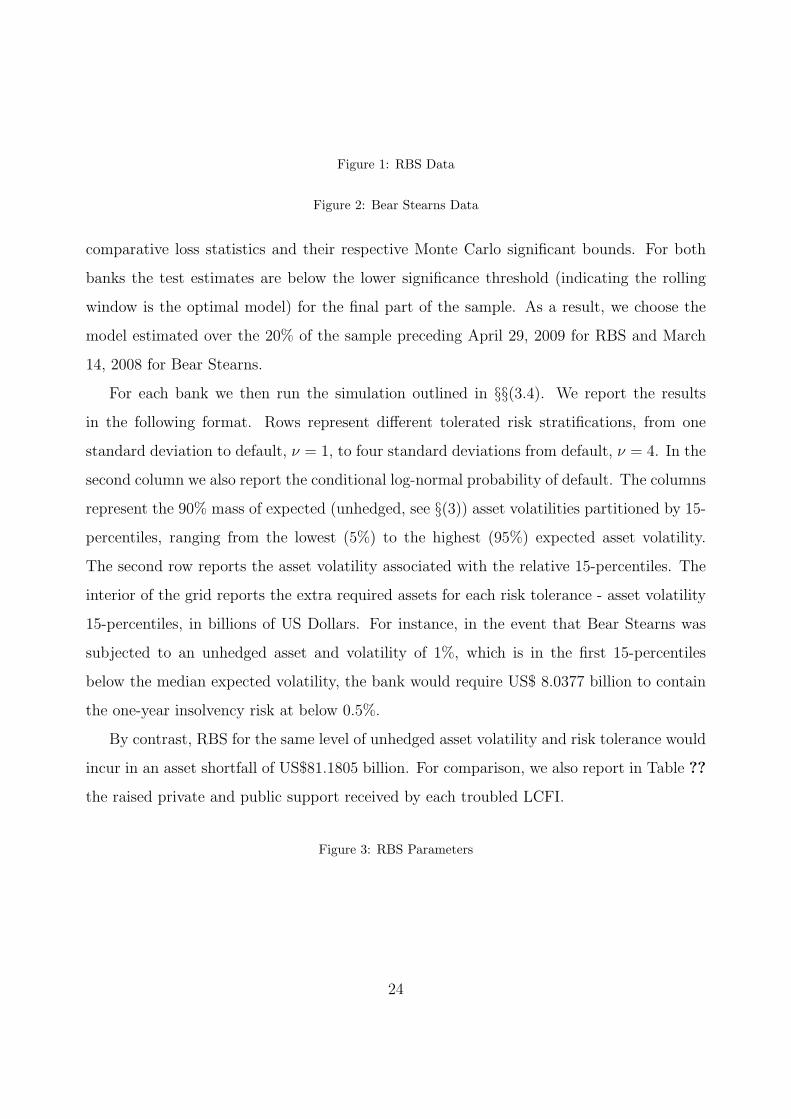
Figure 1: RBS Data

Figure 2: Bear Stearns Data

comparative loss statistics and their respective Monte Carlo significant bounds. For both

banks the test estimates are below the lower significance threshold (indicating the rolling

window is the optimal model) for the final part of the sample. As a result, we choose the

model estimated over the 20% of the sample preceding April 29, 2009 for RBS and March

14, 2008 for Bear Stearns.

For each bank we then run the simulation outlined in §§(3.4). We report the results

in the following format. Rows represent different tolerated risk stratifications, from one

standard deviation to default, ν = 1, to four standard deviations from default, ν = 4. In the

second column we also report the conditional log-normal probability of default. The columns

represent the 90% mass of expected (unhedged, see §(3)) asset volatilities partitioned by 15-

percentiles, ranging from the lowest (5%) to the highest (95%) expected asset volatility.

The second row reports the asset volatility associated with the relative 15-percentiles. The

interior of the grid reports the extra required assets for each risk tolerance - asset volatility

15-percentiles, in billions of US Dollars. For instance, in the event that Bear Stearns was

subjected to an unhedged asset and volatility of 1%, which is in the first 15-percentiles

below the median expected volatility, the bank would require US$ 8.0377 billion to contain

the one-year insolvency risk at below 0.5%.

By contrast, RBS for the same level of unhedged asset volatility and risk tolerance would

incur in an asset shortfall of US$81.1805 billion. For comparison, we also report in Table ??

the raised private and public support received by each troubled LCFI.

Figure 3: RBS Parameters

24

Figure 4: Bear Stearns Parameters

Figure 5: RBS Comparative Loss Statistic

5. Results and Analysis

5.1. Analysis of Dynamic Correlations

The objective of our analysis is to forecast the volatility of assets and its conditional

quadratic covariation with the benchmark CDS indices. The VAR-MV-GARCH model cap-

tures time varying dependency in both direction and variation of the dynamic equations of

interest (in our case equity, CDX and iTraxx). The employment of the VAR-MV-GARCH

model allows for the estimation and testing of volatility transmission between the elements

entering the VAR. The results from VAR-MV-GARCH models are presented in Appendix

B. The vast majority of the estimated coefficients are statistically significant and there is

no evidence of statistical misspecification. The results indicate a strong negative correlation

between both indices and institutional equity and more importantly when the correlation of

returns between the indices increases there is a marked rise in the negative correlation be-

tween equity returns of banks and the indices. Exclusion restrictions to establish the linear

independence of equity returns and the evolution of the indices were decisively rejected in

all cases establishing thus the empirical validity of the estimated model.

From the estimated coefficients we calculate the time evolution of the conditional volatil-

ities and associated correlation coefficients. On the basis of these estimates, we also compute

the value of the assets (Figure E.13), the imputed volatility (Figure E.17), the D-to-D (figure

E.15) and the subsequent probability of default (figure E.16) for the sixteen LCFIs. For ease

of presentation, the results are disaggregated based primarily on geography. As such, we

follow a nationality grouping classification criteria as indicated by obvious divisions between

US, UK, Swiss/German and French LCFIs. It can be seen that the time evolution of equity

volatility exhibits common characteristics across LCFI’s and, as expected, the conditional

Figure 6: Bear Stearns Comparative Loss Statistic

25

correlation with equity is consistently negative with both indices. However, there are subtle

differences in these patterns both in terms of magnitude and more importantly in terms of

the timing that changes in direction and intensity occur.

Beginning the discussion of the results with the group of US-based LCFIs, the path of

the conditional equity volatility displays a modest upward movement since August 2007,

following a very flat trajectory in the sub-period sample preceding the crisis. We can also

see that asset volatility peaks up very rapidly by the last quarter of 2008. For pure invest-

ment banks such as Goldman Sachs, Merrill Lynch and Morgan Stanley, the peaked values

range between .1 and .2 and they subsequently decline to lower levels, albeit still-elevated

compared to their pre-crisis peak values. Unsurprisingly, for Lehman Brothers the increase

is of exceptional magnitude as it is equal to 1.1, a five-fold increase compared to its peers.

At the same time the conditional correlations of the equity value for the three survived

investment banks with both the CDX and the iTraxx are negative throughout the entire

sample period and show an accelerating negative trend in early 2008. Such trend does not

dissipate even in early 2009 and demonstrates that there is a very clear pattern of feedback

effects between the CDS index market and the equity market value of these institutions. In

particular, such relationship becomes more pronounced over the financial crisis period with

an average correlation value rising almost continuously from the beginning of 2005 through

the first quarter of 2009, by which time correlation levels have increased from -.25 to -.6.

The estimated conditional correlation from the model also shows that for Lehman Brothers

correlations are relatively steady over the period starting from a substantially higher value

of approximately -.4. The Lehman collapse causes the largest increase of co-movements

between these variables.

It is important to note that at the beginning of the sample the correlation between the

equity and the CDX index tends to exceed that with the iTraxx but then this relationship

encounters a potential break during the onset of the subprime crisis, then the relative dom-

inance of the CDX almost disappears and the relative weight of the two indices becomes

virtually indistinguishable. Citigroup follows approximately the same pattern but with a

higher intensity as the maximum equity volatility reaches .35 and the correlation with both

26

indices reaches -.8. The findings also suggest that Bear Stearns equity volatility sharply

explodes in the first quarter of 2008 picking up to around 0.6, with negative conditional

correlations sharply reversing their downward trend during 2007.

Within the group of UK LCFIs, noticeably RBS exhibits the highest equity volatility,

with a value of .35, compared to relatively contained levels for HSBC (.1) and for Barclays

(.2). Thus, the equity volatility of RBS spikes dramatically during 2008, but then essen-

tially, following the UK Government’s financial support for RBS, returns to its pre-crisis

pattern. Note also that there are no major changes in the conditional correlations although

quite remarkably the average correlation of equity for the UK banks with the iTraxx index

precipitously jumps at an elevated level.

Our estimates of the conditional equity volatility of continental European banks are

substantially lower with the maximum values not exceeding .1. The volatility paths followed

by BNP Paribas, Societe Generale and UBS display a very modest upward trend and do show

abrupt upwards movements, whilst the volatility patterns observed for Deutsche Bank and

Credit Suisse track closely the levels experienced by the US and the UK institutions. With

the exception of UBS, the average correlation across the indices is of the same magnitude

and is in line with the evolution of the other two banks. Remarkably, in the case of UBS

the conditional correlation remains negative throughout the whole period and starting from

a relatively important level (-.4) declines steadily after August 2007 end ends the sample

period at just above zero.

Overall, the average correlation between the indices increases from approximately .4 (its

average pre-crisis value) to a value in excess of .6, whilst the correlation between the indices

and equity returns becomes more pronounced with an average value of -.6 compared to -.25.

Such patterns are observed uniformly across all the banks and constitute strong evidence of

detrimental volatility transmission between the evolution of the indices and the equity of all

the banks included in this study. It is the uniformity of reaction, both in terms of size and

direction to the same shock that constitutes a severe threat to the stability of the banking

system.

For all sixteen LCFIs the resulting CDPs increase very sharply during 2008. These indi-

27

cators therefore show that when the subprime crisis begins to evolve into a global financial

crisis the average dependence among the global sample of banks equity and CDS indices

enters an accelerating phase that reaches a peak towards the end of 2008. This finding is

consistent with the evidence presented in a recent study by Longstaff (2010) who finds a

rapid increase in cross-financial markets linkages as the subprime crisis developed.

From a visual inspection, the banks included in this study, in principle, clearly divide

into two groups: the US and UK LCFIs AND the continental European LCFIs, the dif-

ference being the height of the jump of the default probability at the peak of the crisis in

the wake of the Lehman Brothers bankruptcy. For several US banks the CDP rises to 35%

whilst for the European block the CDP are generally not greater than 25%. In the UK for

HSBC the relevant probability is just above 5% (on an annual basis) whilst, not surprisingly,

whilst Barclays and RBS are subject to substantial increases to default probability. More

specifically, this value for RBS far exceeds 35%, rendering the bank totally dependent on

government support to ensure its survival. After the announcement of in-all-but-name na-

tionalization of the bank, the associated probability of default reverts sharply to safe levels.

The results also show significant dissimilarities in the probability of default between the US

institutions as some of them show distinct reductions, whilst for others the probability of

default increases over the latest part of the period under consideration. More specifically,

the distress indicators clearly shows that for Citigroup, Bank of America and Morgan Stan-

ley default risk continue to increase much above the historical trend, in the aftermath of

Lehman Brothers’ default. At the other hand of the spectrum, LCFIs, such as Goldman

Sachs and J. P. Morgan, are about equally less vulnerable to pullover effects from the CDS

market and hence more resilient to the liquidity crisis. Overall, the results indicate that

systemic bank risks and CD market shocks appear to be highly dependent. These results

are also consistent with those found in other studies (see, the IMF (2009, a, b)).

Stress testing involves hypothesizing changes in the aggregate volatility of the banks’

assets and gives a simple measure of potential risk vectors in their aggregate form. These

types of measures should prevent banks from leveraging themselves to a point whereby they

are extremely vulnerable to changes in asset volatility, which would then require costly

28

readjustments, possibly forcing a bank below some critical solvency thresholds

5.2. Analysis of D-2-D Injections (Stress Testing)

In view of the econometric evidence, we proceed by conducting a bank stress-testing

exercise for a given value of the liabilities to evaluate the imputed adequate bank capital

requirements to ensure the soundness of each institution. Such a strong assumption is jus-

tified in the current circumstances because their valuation is more accurate when compared

to the valuation of assets. A stress test exercise involves hypothesizing changes in the ag-

gregate volatility of the banks’ assets and gives a simple measure of potential risk vectors

in their aggregate form. These types of measures should prevent banks from leveraging

themselves to a point whereby they are extremely vulnerable to changes in asset volatility,

which would then require costly readjustments, possibly forcing a bank below some critical

solvency thresholds.

5.3. Asset Volatility and Required Capital Injections

The results are presented in figures D.8-D.10. The limiting D-to-D is denoted by the

horizontal line that marks the associated D-to-D for each bank given the imposed 1% proba-

bility to default as the maximum tolerated stay requirement before a regulator could decide

to impose a contingent capital surcharge following a distress event. These figures associate

the required increase in the value of equity for any realised value of asset volatility condi-

tional on a fixed value of liabilities. The analysis is necessarily aggregate and stylized, and is

not intended to substitute for detailed analysis of the needs of specific institutions’ business

activities or portfolios.

The required capital injections estimates, computed using the D-to-D methodology, need

the following qualification. The assets are assumed to be drawn from a pool that preserves

the overall level of volatility and capital injections by governments are considered almost

risk-less and therefore will reduce the accumulation of balance sheet risks. Whether the

re-payment level on these assets is recognized as a liability is a current point of debate in

policy circles, particularly in the US and the UK.

29

A key aspect of the study is that stress-test indicators can show moves to medium- and

high-volatility states and hence can be used to assess the degree of current banking fragility

and uncertainty. Such indicators may also be useful in establishing whether and when a

systemic crisis is subsiding, particularly if the low-volatility state persists, and thus when

the withdrawal supportive crisis measures can be safely considered.

The volatility estimates are obtained from Monte-Carlo simulations using the estimated

coefficients from the multivariate GARCH model. They are sorted in deciles with the exclu-

sion of the tails immediately above the 2.5% cut-off. A close inspection of the range of the

projected asset volatility values reveals substantial differences across financial institutions.

Of those US LCFIs able to survive the crisis, Bank of America exhibits the largest degree of

variability of asset volatility, ranging from .019 to 0.15, whilst unsurprisingly the institution

with the narrowest dispersion is Goldman Sachs whose upper deciles remain below 0.079.

The estimated asset volatilities for Citigroup, J.P. Morgan and Morgan Stanley are shown

here to range between 0.018 and .11. By contrast, the asset volatility range for European

LCFIs is rather narrow, with the exception of RBS whose volatility range reaches 0.077

exceeding by far the upper limit of the other European institutions. Such wide variations

clearly underscore substantial differences in the resilience of LCFI to withstand identical

adverse-case scenarios. A slight increase in volatility from a given overall safe level results

in differing additional capital requirements for the sixteen institutions included in our sam-

ple. Overall, the main takeaway from our simulations is that the ’average’ asset volatility

of US-based LCFIs is substantially higher compared to non-US institutions. With such

system-wide heterogeneity across institutions the development of common prudential regu-

latory standards aimed at protecting banks solvency may prove somewhat problematic and

thus the implementation of reliable tools for this task should proceed expeditiously.

The magnitudes of the effects are nontrivial. Indeed, with respect to the US institutions,

we find that for only a rather narrow range of asset volatilities they are able to comply with

the imposed safety requirement. Morgan Stanley, Citigroup, J.P. Morgan and Goldman

Sachs require no further capital injections provided that asset volatility does not exceed

0.002. This finding is noteworthy as this value represents the lowest of deciles in the empir-

30

ical volatility distribution derived from our simulations. The results indicate that a severe

deterioration of market conditions resulting in higher asset volatility will augment aggre-

gate banking system capital needs. Assuming that all the US LCFIs were to experience

the same level of asset volatility of 0.04, a value consistent with the mid-decile of the em-

pirical distribution, the needed funds for a complete bank recapitalization will be roughly

$300bn. Interestingly, the most vulnerable institutions appear to be Bank of America and

J.P. Morgan requiring $150bn each whereas the individual capital injections for bank holding

companies such as Goldman Sachs and Morgan Stanley stand at $40bn and $50bn, respec-

tively. Furthermore, if each individual institution were subject to the ’mode’ of the empirical

asset volatility distribution, which corresponds to the fourth decile, then the required capital

adequacy, surcharges are statistically and economically significant. Specifically, we project

such injections ranging from $250bn required for Bank of America to $40bn for Goldman

Sachs.

In striking contrast, BNP Paribas and Societe Generale, the two French LCFIs in the

sample, appear to be relatively safe within the limits of their volatility distributions as no

capital injections are required for asset volatility levels not exceeding the fourth decile. Even

in presence of rather adverse volatility regimes the size of capital cushions does not exceed

$200bn. The Swiss and German banks appear somewhat more vulnerable to realisations of

volatility in excess of the third decile, although conditions have to substantially deteriorate

to absorb extra capital in the case of Deutsche Bank. This finding indicates that for realised

asset volatility at the ’mode’ these banking institutions will face a capital shortfall of $160bn.

As such, this should be viewed as indicative of the recapitalization needs by these banks to

stabilize this segment of the European banking system.

Focusing next on the UK based-LFCIs, the results show a mixed pattern. Interestingly,

HSBC appears to be the most resilient institution. For the first two deciles of volatility

no further equity is needed to meet the policy objective, whilst at ‘mode’ $100bn will be

required. In contrast, Royal Bank of Scotland seems to be one of the more vulnerable

LCFIs as reflected in its higher capital requirements. Our calculations suggest that if asset

volatility reaches the specific threshold requirement, capital injections would need to be some

31

$200bn whilst a more demanding level of volatility - standing at a ’mode’ intensity -raises the

amount of capital to be injected to around $260bn. Barclays experiences a wide range within

its volatility distribution suggesting no call for extra capital. However, a higher volatility

scenario for the bank - asset volatility at mode value of 0.017- will push up considerably the

recapitalization needs, possibly totalling $100bn.

Overall, our stress-testing results clearly highlight the dangers of significant losses, as a

relatively large number of LCFIs are not adequately capitalized and individually capable of

surviving reasonable stress events. The deterioration of the quality of assets signalled by

conditions in the CDS index market points to comparatively substantial capital injections

required to restore banks’ balance sheets to health. Notably for most European banks there

is a reasonably wide range of asset volatilities for which additional equity is not needed to

cushion potential writedowns. In contrast, for the US banks the ‘safe range’ of volatilities is

somewhat narrow. Not surprisingly, given the common heavy exposure of these institutions

to subprime-mortgage related securities, what emerges from this exercise is that in absence

of rigorous policy measures to address troubled assets, the banks included in this study

(with the notable exception of HSBC) enter the ‘insolvency state’. However, in some cases

this distress proves to be relatively short-lived. Thus, the empirical evidence underscore

that capital adequacy for systemically important financial institutions remains fractured in

response to CDS index market shocks.

Remaining in a high-volatility regime for long could indicate a serious threat to the

stability of the banking system. Consequently, there is clear evidence that the resilience

of the banking sector is conditional upon a sustained improvement to the banks’ balance

sheets. As a result, there remains considerable scope for further fresh capital infusions for

LCFIs.

Thus, these results are consistent with the emerging consensus that the long-term viabil-

ity of institutions needs to be revaluated to assess both prospects for further write downs and

potential capital needs. Without a thorough cleansing of banks’ balance sheets of impaired

assets, accompanied by restructuring and, where needed, recapitalization, risks remain that

banks’ problems will continue to exert upward pressure on systemic risk. Without making a

32

judgment about the appropriateness of our asset volatility scenarios, it is important to note

that these amounts are ’inflated’ to the degree that governments have guaranteed banks

against further losses of some of the bad assets on their balance sheets.

Furthermore, if we consider a more conservative regulatory approach establishing the

maximum tolerated default probability below 1% almost all of the institutions included in

this study will be in need of substantial additional equity injections from governments. For

any given safety limit the key information provided by developments in the CRT market

provide a valuable signal to the authorities about the additional capital requirements for

each financial institution and more importantly about the overall fragility of the banking

system.

In summary, these results do provide evidence that observing shifts in asset volatility

regimes using the CDX and iTraxx indices as aggregating measures of corporate default risk

can be helpful in detecting the degree to which the financial system is suffering a systemic

event.

6. Concluding Remarks

Bank default risk is currently the predominant issue of concern to academic, financial

practitioners and policymakers across the world. The recent failure of several LCFIs illus-

trates that the too big to fail paradigm predominant in the analysis of financial stability of

large mainstream commercial and investment banks is no longer valid. We approach the

issue of the stability of the banking sector by studying the potential effects of CDs on the

statistical moments of the equity of LFCIs.

This paper offers a concrete illustration of the direct links between the global banking

system and the CDs index market. We propose a set of models and empirical tests for

predicting the current and future linkages between various CD markets and financial in-

stitutions. Specifically, we jointly model the evolution of equity returns and asset return

volatility of 16 systemically important LCFIs, using a VAR-MV-GARCH model, with the

evolution of the two standardized CDS indices. The conditional equity volatilities are used

to impute the value and volatility of assets using a Merton type model.

33

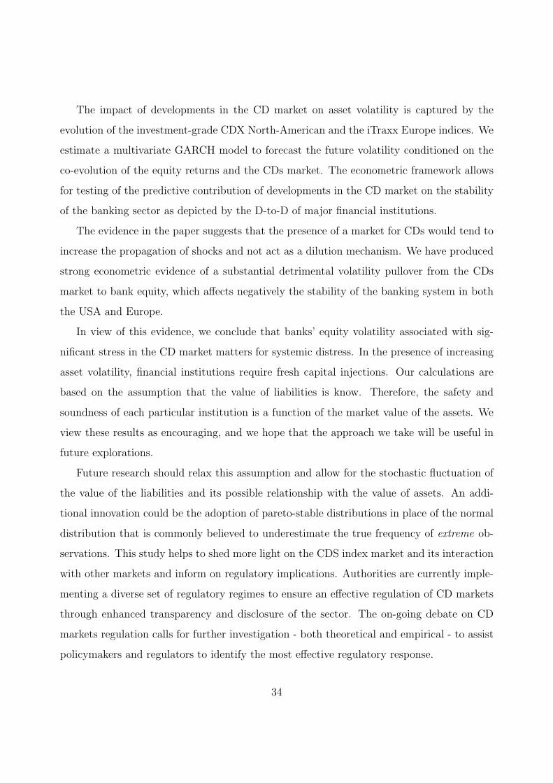
The impact of developments in the CD market on asset volatility is captured by the

evolution of the investment-grade CDX North-American and the iTraxx Europe indices. We

estimate a multivariate GARCH model to forecast the future volatility conditioned on the

co-evolution of the equity returns and the CDs market. The econometric framework allows

for testing of the predictive contribution of developments in the CD market on the stability

of the banking sector as depicted by the D-to-D of major financial institutions.

The evidence in the paper suggests that the presence of a market for CDs would tend to

increase the propagation of shocks and not act as a dilution mechanism. We have produced

strong econometric evidence of a substantial detrimental volatility pullover from the CDs

market to bank equity, which affects negatively the stability of the banking system in both

the USA and Europe.

In view of this evidence, we conclude that banks’ equity volatility associated with sig-

nificant stress in the CD market matters for systemic distress. In the presence of increasing

asset volatility, financial institutions require fresh capital injections. Our calculations are

based on the assumption that the value of liabilities is know. Therefore, the safety and

soundness of each particular institution is a function of the market value of the assets. We

view these results as encouraging, and we hope that the approach we take will be useful in

future explorations.

Future research should relax this assumption and allow for the stochastic fluctuation of

the value of the liabilities and its possible relationship with the value of assets. An addi-

tional innovation could be the adoption of pareto-stable distributions in place of the normal

distribution that is commonly believed to underestimate the true frequency of extreme ob-

servations. This study helps to shed more light on the CDS index market and its interaction

with other markets and inform on regulatory implications. Authorities are currently imple-

menting a diverse set of regulatory regimes to ensure an effective regulation of CD markets

through enhanced transparency and disclosure of the sector. The on-going debate on CD

markets regulation calls for further investigation - both theoretical and empirical - to assist

policymakers and regulators to identify the most effective regulatory response.

34

References

[1] Allen, F. and E. Carletti (2006). Credit risk transfer and contagion. Journal of Monetary Eco-

nomics 53 (1), 80–111.

[2] Allen, F. and D. Gale (2000). Financial contagion. Journal of Political Economy Vol. 108 (1), 1–33.

[3] Baur, D. and E. Joossens (2006). The effect of credit risk transfer on financial stability. EUR Working

Paper Series No. 21521.

[4] Black, F. and M. Scholes (1973). Pricing of options and corporate liabilities. Journal of Political

Economy 81 (3), 637–659.

[5] Blanco, R., S. Brennan, and I. W. Marsh (2005). An empirical analysis of the dynamic relationship

between investment-grade bonds and credit default swaps. Journal of Finance Vol. 63 (2), 2255–2281.

[6] Buraschi, A., P. Porchia, and F. Porchia (2010). Correlation risk and optimal portfolio choice. Journal

of Finance Vol. 65 (1), 393–420.

[7] Bystrom, H. N. E. (2005). Credit default swaps and equity prices: The iTraxx CDS index market. Lund

University Working Paper Series.

[8] Duffie, D. (July 2008). Innovations in credit risk transfer: Implications for financial stability. BIS

Working Paper No. 255 .

[9] Engle, R. F. and K. F. Kroner (1995). Multivariate simultaneous generalized ARCH. Econometric

Theory 11 (1), 122–150.

[10] et al., A. B. (2005). Measuting default risk premia from default swap rates and edfs. Stanford University

Working Paper .

[11] Giacomini, R. and H. White (2006). Tests of conditional predictive ability. Econometrica 74 (6),

1545–1578.

[12] Gropp, R., J. Vesala, and G. Vulpes (2006). Equity and bond market signals as leading indicators of

bank fragility. Journal of Money, Credit and Banking 38 (2), 399–428.

[13] Hawkesby, C., I. W. Marsh, and I. Stevens (2003). Comovements in the prices of securities issued by

large complex financial institutions. Bank of England: Financial Stability Review: Dec 2003 , 91–101.

[14] Hu, H. T. C. and B. Black (2008). Debt, equity, and hybrid decoupling: Governance and systemic risk

implications. European Financial Management 14 (4).

[15] Lehar, A. (2005). Measuring systematic risk: A risk management approach. Journal of Banking and

Finance 29 (10), 2577–2603.

[16] Longin, F. M. and B. Solnik (2001). Extreme correlations of international equity markets during

extremely volatile periods. Journal of Finance 56 (2), 649–676.

[17] Merton, R. C. (1974a). On the pricing of corporate debt: The risk structure of interest rates,”. Journal

of Finance 29 (2), 449–70.

35

[18] Merton, R. C. (1974b). Theory of rational option pricing. Bell Journal of Economics 4 (1), 141–83.

[19] Morrison, A. D. (2005). Credit derivatives, disintermediation, and investment decisions. Journal of

Business 78 (2), 621–648.

[20] of England, B. (2001). Financial stability review. Bank of England Publications No. 11, 137–159.

[21] Wagner, W. and I. Marsh (2006). Credit risk transfer and financial sector stability. Journal of Financial

Stability 2 (2), 173–193.

[22] Zhu, H. (2006). An empirical comparison of credit spreads between the bond market and the credit

default swap market. Journal of Financial Services Research 29 (3), 211–235.

36

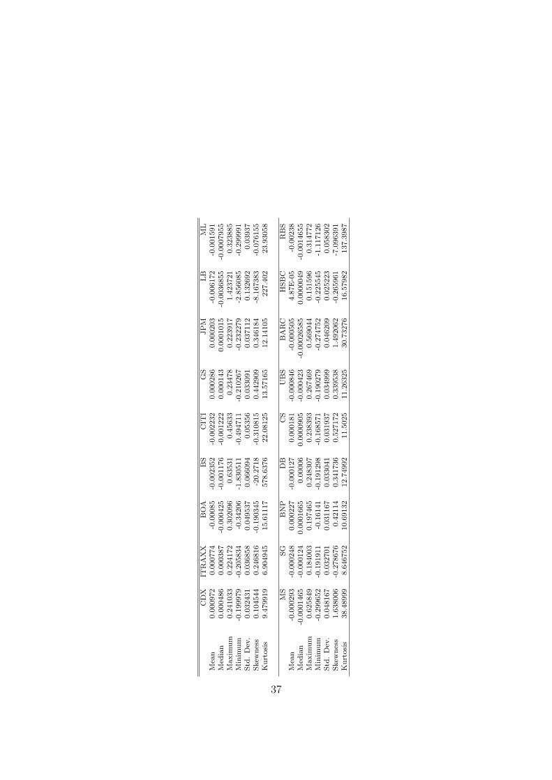
CD

XIT

RA

XX

BO

AB

SC

ITI

GS

JP

MLB

ML

Mea

n0.0

00972

0.0

00774

-0.0

0085

-0.0

02352

-0.0

02232

0.0

00286

0.0

00203

-0.0

06172

-0.0

01591

Med

ian

0.0

00486

0.0

00387

-0.0

00425

-0.0

01176

-0.0

01222

0.0

00143

0.0

001015

-0.0

036855

-0.0

007955

Maxim

um

0.2

41033

0.2

24172

0.3

02096

0.6

3531

0.4

5633

0.2

3478

0.2

23917

1.4

23721

0.3

23885

Min

imum

-0.1

99979

-0.2

05834

-0.3

4206

-1.8

30511

-0.4

94711

-0.2

10267

-0.2

32279

-2.8

56085

-0.2

99991

Std

.D

ev.

0.0

32431

0.0

36858

0.0

49537

0.0

66094

0.0

5356

0.0

33091

0.0

37112

0.1

32692

0.0

3937

Skew

nes

s0.1

04544

0.2

46816

-0.1

90345

-20.2

718

-0.3

10815

0.4

42909

0.3

46184

-8.1

67383

-0.0

76155

Kurt

osi

s9.4

79919

6.9

04945

15.6

1117

578.6

376

22.0

8125

13.5

7165

12.1

4105

227.4

02

23.9

3058

MS

SG

BN

PD

BC

SU

BS

BA

RC

HSB

CR

BS

Mea

n-0

.000293

-0.0

00248

0.0

00227

-0.0

00127

0.0

00181

-0.0

00846

-0.0

00505

4.8

7E

-05

-0.0

0238

Med

ian

-0.0

001465

-0.0

00124

0.0

001665

0.0

0006

0.0

000905

-0.0

00423

-0.0

0026585

0.0

000049

-0.0

014655

Maxim

um

0.6

25849

0.1

84003

0.1

97465

0.2

48307

0.2

38393

0.2

67469

0.5

69044

0.1

51596

0.3

14772

Min

imum

-0.2

99652

-0.1

91911

-0.1

6141

-0.1

91298

-0.1

68571

-0.1

90279

-0.2

74752

-0.2

25545

-1.1

17126

Std

.D

ev.

0.0

48167

0.0

32701

0.0

31167

0.0

33041

0.0

31937

0.0

34999

0.0

46209

0.0

25223

0.0

58302

Skew

nes

s1.6

38006

-0.2

78676

0.4

2114

0.3

41736

0.5

27172

0.3

39538

1.4

92062

-0.2

65961

-7.0

96391

Kurt

osi

s38.4

8999

8.6

46752

10.6

9132

12.7

4992

11.5

025

11.2

6325

30.7

3276

16.5

7982

137.3

987

37

Mar

ket

Cap

ital

isat

ion

Tot

alL

iabi

litie

s

July

1,20

07Se

ptem

ber

1,20

08Ja

nuar

y1,

2009

Apr

il1,

2009

July

1,20

07Se

ptem

ber

1,20

08Ja

nuar

y1,

2009

Apr

il1,

2009

Ban

kof

Am

eric

a21

0419

.313

4751

.242

062.

9645

129.

7715

6894

3000

1640

8910

0019

9185

5000

1991

8550

00B

ear

Stea

rns

1407

6.55

1359

.36

1359

.36

1359

.36

3821

0510

038

2105

100

3821

0510

038

2105

100

Cit

igro

up23

1664

.885

764.

8119

345.

8614

774.

2920

7403

3000

1796

8400

0017

0167

3000

1701

6730

00G

oldm

anSa

chs

7640

152

379.

9737

279.

8450

930.

1510

6555

4000

8101

7600

076

9330

900

7693

3090

0J.

P.M

orga

n14

8925

.214

0024

.895

212.

3810

5747

.814

3892

6000

2008

1680

0018

6662

4000

1866

6240

00L

ehm

anB

roth

ers

3290

8.72

206.

728

.59

28.9

466

6264

100

6662

6410

066

6264

100

6662

6410

0M

erri

llL

ynch

6375

9.15

3392

9.93

1862

0.86

1862

0.86

9881

1800

064

7540

000

6475

4000

064

7540

000

Mor

gan

Stan

ley

6722

6.06

3182

8.69

2173

7.09

2549

7.83

1014

1400

0060

7981

100

7186

8210

071

8682

100

Soci

ete

Gen

eral

e81

340.

4446

690.

3824

520.

5822

893.

3414

2002

5000

1584

6350

0013

5105

8000

1288

4920

00B

NP

Par

ibas

1047

97.3

7479

4.88

3507

5.99

3969

6.98

2235

9350

0029

3618

1000

2734

7270

0026

0808

3000

Deu

tsch

eB

ank

7291

2.44

3901

9.4

1499

6.36

2565

8.12

2706

4470

0031

5425

4000

2023

3360

0019

2963

7000

Cre

dit

Suis

se80

794.

2548

859.

8629

155.

9937

946.

8510

7615

6000

1008

7240

0091

5058

400

8531

2200

0U

BS

1182

13.9

4347

2.52

3698

8.34

2854

9.78

1850

6140

0017

8207

6000

1205

4410

0011

2385

0000

Bar

clay

s92

987.

2544

507.

6612

809.

8918

928.

1624

2509

2000

3609

1860

0018

9516

7000

1963

5790

00H

SBC

2182

7117

9570

.495

115.

3110

1632

2267

0300

0029

8460

9000

1977

7780

0020

4917

1000

RB

S11

3854

.555

514.

9612

514.

6920

347.

0936

7018

4000

4162

3200

0022

9294

6000

2375

7170

00

38

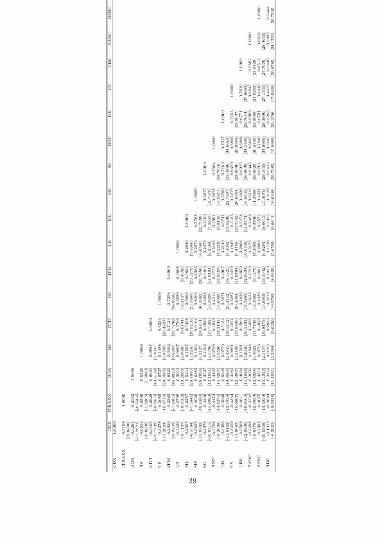
CD

XIT

RA

XX

BO

AB

SC

ITI

GS

JPM

LB

ML

MS

SG

BN

PD

BC

SU

BS

BA

RC

HSB

CR

BS

CD

X1.0

000

ITR

AX

X0.5

198

1.0

000

[19.6

436]

BO

A-0

.3294

-0.2

562

1.0

000

[-11.2

621]

[-8.5

564]

BS

-0.0

213

-0.0

595

0.0

525

1.0

000

[-0.6

900]

[-1.9

265]

[1.6

983]

CIT

I-0

.3165

-0.2

928

0.8

031

0.0

987

1.0

000

[-10.7

739]

[-9.8

856]

[43.5

134]

[3.2

047]

GS

-0.3

278

-0.3

085

0.6

727

0.1

488

0.6

334

1.0

000

[-11.2

024]

[-10.4

715]

[29.3

505]

[4.8

595]

[26.4

227]

JPM

-0.2

939

-0.2

385

0.8

125

0.0

192

0.7

124

0.7

258

1.0

000

[-9.9

259]

[-7.9

305]

[44.9

933]

[0.6

203]

[32.7

780]

[34.0

666]

LB

-0.2

436

-0.2

798

0.3

013

0.0

897

0.2

706

0.3

589

0.2

808

1.0

000

[-8.1

107]

[-9.4

102]

[10.2

003]

[2.9

080]

[9.0

741]

[12.4

147]

[9.4

450]

ML

-0.2

557

-0.2

287

0.5

414

0.1

597

0.5

438

0.5

869

0.5

824

0.2

846

1.0

000

[-8.5

394]

[-7.5

844]

[20.7

895]

[5.2

250]

[20.9

210]

[23.3

989]

[23.1

279]

[9.5

866]

MS

-0.3

235

-0.3

026

0.6

383

0.1

294

0.6

104

0.8

203

0.6

385

0.2

974

0.5

768

1.0

000

[-11.0

362]

[-10.2

488]

[26.7

694]

[4.2

127]

[24.8

811]

[46.3

082]

[26.7

850]

[10.0

580]

[22.7

969]

SG

-0.2

978

-0.4

236

0.3

527

0.1

102

0.3

920

0.4

258

0.3

463

0.2

478

0.2

190

0.3

675

1.0

000

[-10.0

715]

[-15.0

988]

[12.1

681]

[3.5

798]

[13.7

562]

[15.1

929]

[11.9

191]

[8.2

584]

[7.2

453]

[12.7

570]

BN

P-0

.2758

-0.4

174

0.4

102

0.0

790

0.4

029

0.4

214

0.3

722

0.2

183

0.2

094

0.3

878

0.7

684

1.0

000

[-9.2

638]

[-14.8

273]

[14.5

207]

[2.5

596]

[14.2

138]

[15.0

009]

[12.9

457]

[7.2

219]

[6.9

145]

[13.5

811]

[38.7

616]

DB

-0.3

386

-0.3

929

0.5

249

0.0

770

0.5

184

0.5

871

0.4

907

0.2

149

0.3

741

0.5

760

0.7

199

0.7

317

1.0

000

[-11.6

162]

[-13.7

939]

[19.9

066]

[2.4

945]

[19.5

712]

[23.4

152]

[18.1

825]

[7.1

062]

[13.0

236]

[22.7

497]

[33.4

860]

[34.6

610]

CS

-0.3

450

-0.4

364

0.3

583

0.0

991

0.3

974

0.5

287

0.3

479

0.1

949

0.3

155

0.5

279

0.6

670

0.6

806

0.7

155

1.0

000

[-11.8

687]

[-15.6

607]

[12.3

907]

[3.2

169]

[13.9

806]

[20.1

064]

[11.9

794]

[6.4

156]

[10.7

342]

[20.0

654]

[28.8

990]

[29.9

903]

[33.0

607]

UB

S-0

.3508

-0.4

641

0.4

004

0.1

591

0.4

569

0.4

826

0.3

652

0.2

968

0.3

478

0.4

626

0.6

915

0.6

988

0.6

771

0.7

610

1.0

000

[-12.0

930]

[-16.9

166]

[14.1

086]

[5.2

046]

[16.5

834]

[17.7

883]

[12.6

634]

[10.0

349]

[11.9

774]

[16.8

445]

[30.9

039]

[31.5

406]

[29.7

014]

[37.8

683]

BA

RC

-0.2

698

-0.3

732

0.3

695

0.1

048

0.3

426

0.3

532

0.2

720

0.2

179

0.2

482

0.3

319

0.6

345

0.6

837

0.5

959

0.5

547

0.5

887

1.0

000

[-9.0

479]

[-12.9

859]

[12.8

385]

[3.4

022]

[11.7

749]

[12.1

902]

[9.1

275]

[7.2

083]

[8.2

736]

[11.3

588]

[26.5

025]

[30.2

430]

[23.9

585]

[21.5

253]

[23.5

128]

HSB

C-0

.2982

-0.4

075

0.4

313

0.0

776

0.4

620

0.4

439

0.3

881

0.2

069

0.2

574

0.4

321

0.6

704

0.7

340

0.6

731

0.6

440

0.6

513

0.6

613

1.0

000

[-10.0

859]

[-14.4

050]

[15.4

343]

[2.5

157]

[16.8

179]

[15.9

919]

[13.5

942]

[6.8

294]

[8.6

015]

[15.4

670]

[29.1

653]

[34.8

900]

[29.3

866]

[27.1

755]

[27.7

076]

[28.4

653]

RB

S-0

.1913

-0.2

694

0.3

253

0.0

783

0.2

856

0.3

219

0.2

423

0.1

730

0.2

026

0.3

129

0.5

416

0.5

247

0.5

296

0.4

672

0.5

430

0.5

993

0.5

404

1.0

000

[-6.2

921]

[-9.0

328]

[11.1

051]

[2.5

364]

[9.6

220]

[10.9

785]

[8.0

629]

[5.6

709]

[6.6

811]

[10.6

348]

[20.7

982]

[19.8

969]

[20.1

556]

[17.0

600]

[20.8

780]

[24.1

701]

[20.7

330]

39

Tab

le.4

:B

OA

BS

CIT

IG

SJPM

LB

ML

MS

SG

BN

PD

BC

SU

BS

BA

RC

HSB

CR

BS

z1

,1-0

.0113

-0.0

318

0.0

375

-0.0

244

-0.0

626

-0.0

657

0.0

016

0.0

342

0.1

017

-0.0

138

0.0

305

0.0

891

0.0

862

0.0

048

-0.0

269

-0.0

349

[-0.4

236]

[-0.8

225]

[1.2

636]

[-0.8

893]

[-2.4

093]

[-2.2

901]

[0.0

528]

[1.1

777]

[3.1

936]

[-0.4

429]

[1.0

491]

[2.8

896]

[2.9

669]

[0.1

765]

[-0.8

874]

[-1.1

621]

z1

,2-0

.0254

-0.0

000

-0.0

318

-0.0

643

-0.0

466

-0.0

938

0.0

000

-0.0

185

-0.0

642

-0.0

716

-0.0

576

-0.0

628

-0.0

550

-0.0

590

-0.0

178

-0.0

760

[-1.8

007]

[-0.0

009]

[-2.4

855]

[-3.4

293]

[-2.8

785]

[-2.9

560]

[0.0

192]

[-0.8

380]

[-3.5

811]

[-3.7

117]

[-3.4

689]

[-3.7

513]

[-3.1

389]

[-3.1

565]

[-2.2

219]

[-4.8

168]

z1

,3-0

.0041

0.0

000

-0.0

076

-0.0

464

-0.0

094

0.0

743

-0.0

000

-0.0

120

-0.0

080

0.0

063

-0.0

088

-0.0

104

-0.0

234

-0.0

241

-0.0

152

0.0

292

[-0.2

872]

[0.0

020]

[-0.4

409]

[-2.4

724]

[-0.5

516]

[1.8

530]

[-0.0

136]

[-0.5

116]

[-0.3

921]

[0.2

852]

[-0.4

586]

[-0.5

841]

[-1.1

877]

[-1.0

576]

[-1.4

858]

[1.4

673]

µ1

0.0

002

-0.0

000

0.0

004

0.0

006

0.0

007

0.0

002

-0.0

000

0.0

010

0.0

003

0.0

008

0.0

005

0.0

005

0.0

002

0.0

005

0.0

004

0.0

009

[0.6

588]

[-0.0

392]

[1.0

349]

[1.4

241]

[1.5

715]

[0.2

585]

[-0.0

104]

[1.8

848]

[0.6

782]

[1.5

088]

[1.0

748]

[0.9

706]

[0.4

751]

[1.0

103]

[1.2

968]

[1.6

641]

z2

,1-0

.0531

-0.0

212

-0.0

777

-0.1

242

-0.1

627

0.0

254

-0.1

728

-0.1

090

-0.0

166

-0.0

482

-0.0

560

-0.0

695

-0.0

563

0.0

024

-0.0

360

-0.0

002

[-2.2

633]

[-0.9

547]

[-3.6

325]

[-4.4

690]

[-6.1

065]

[5.4

799]

[-7.9

026]

[-4.6

862]

[-0.5

052]

[-1.3

278]

[-1.6

155]

[-2.0

789]

[-1.9

555]

[0.1

182]

[-0.7

244]

[-0.0

096]

z2

,20.0

017

0.0

338

0.0

058

0.0

414

0.0

018

0.0

119

0.0

105

-0.0

130

0.0

304

0.0

259

0.0

232

0.0

340

0.0

113

0.0

487

0.0

202

0.0

136

[0.0

576]

[0.9

596]

[0.1

761]

[1.3

895]

[0.0

631]

[0.3

737]

[0.3

240]

[-0.3

920]

[0.9

312]

[0.8

035]

[0.7

442]

[1.0

402]

[0.3

431]

[1.4

997]

[0.6

178]

[0.4

211]

z2

,30.3

044

0.3

002

0.2

871

0.2

794

0.2

797

0.3

213

0.2

717

0.2

744

0.2

620

0.2

639

0.2

729

0.2

667

0.2

497

0.2

779

0.2

950

0.2

683

[9.4

887]

[8.2

391]

[8.8

378]

[10.3

164]

[9.0

040]

[10.4

926]

[8.6

611]

[9.3

460]

[8.2

768]

[8.4

261]

[8.9

700]

[8.5

673]

[8.0

932]

[8.6

123]

[9.5

219]

[8.3

167]

µ2

-0.0

004

0.0

003

-0.0

007

-0.0

001

-0.0

003

-0.0

009

0.0

010

-0.0

002

-0.0

003

-0.0

000

-0.0

003

-0.0

002

-0.0

005

-0.0

004

-0.0

002

-0.0

007

[-0.5

762]

[0.3

858]

[-0.9

015]

[-0.2

899]

[-0.4

453]

[-1.1

401]

[1.2

882]

[-0.3

598]

[-0.4

751]

[-0.0

012]

[-0.4

669]

[-0.3

456]

[-0.6

571]

[-0.5

610]

[-0.2

381]

[-0.8

107]

z3

,1-0

.0227

-0.0

656

-0.0

310

-0.1

158

-0.0

935

0.0

251

-0.2

067

-0.0

849

-0.0

492

-0.0

558

-0.0

674

-0.1

078

-0.0

563

-0.0

195

-0.0

551

0.0

001

[-1.3

274]

[-3.8

388]

[-1.8

029]

[-2.7

896]

[-4.2

327]

[5.9

592]

[-11.0

947]

[-4.1

392]

[-1.6

915]

[-1.9

543]

[-2.4

214]

[-3.6

780]

[-2.1

120]

[-0.9

659]

[-1.4

221]

[0.0

099]

z3

,20.1

699

0.2

249

0.1

806

0.1

625

0.1

897

0.1

777

0.1

960

0.1

772

0.1

910

0.1

959

0.1

895

0.1

806

0.1

877

0.2

061

0.1

892

0.1

939

[8.1

896]

[8.3

999]

[7.8

573]

[5.0

805]

[9.1

551]

[8.7

253]

[7.7

854]

[8.0

724]

[8.1

770]

[8.7

984]

[9.1

738]

[8.1

333]

[8.3

862]

[9.0

631]

[7.9

232]

[8.5

376]

z3

,30.0

207

0.0

868

-0.0

080

0.0

592

-0.0

101

0.0

158

-0.0

516

0.0

246

-0.0

187

-0.0

087

-0.0

243

-0.0

240

-0.0

202

-0.0

161

-0.0

021

-0.0

001

[0.7

001]

[2.7

802]

[-0.2

678]

[1.1

994]

[-0.3

585]

[0.5

181]

[-1.5

831]

[0.8

470]

[-0.6

191]

[-0.2

927]

[-0.8

235]

[-0.8

244]

[-0.6

684]

[-0.5

277]

[-0.0

657]

[-0.0

061]

µ3

-0.0

003

0.0

001

-0.0

006

0.0

001

-0.0

005

-0.0

009

0.0

011

-0.0

000

-0.0

000

-0.0

000

-0.0

003

-0.0

001

-0.0

003

-0.0

003

-0.0

001

-0.0

003

[-0.4

649]

[0.1

077]

[-0.8

248]

[0.0

977]

[-0.7

388]

[-1.3

049]

[1.2

223]

[-0.1

055]

[-0.1

289]

[-0.1

046]

[-0.5

257]

[-0.1

985]

[-0.4

215]

[-0.4

229]

[-0.1

319]

[-0.3

982]

40

Tab

le.5

:B

OA

BS

CIT

IG

SJPM

LB

ML

MS

SG

BN

PD

BC

SU

BS

BA

RC

HSB

CR

BS

k1

,10.0

015

-0.0

000

0.0

023

0.0

014

0.0

014

0.0

002

0.0

000

0.0

021

0.0

027

0.0

025

0.0

020

0.0

025

0.0

017

0.0

020

-0.0

001

0.0

030

[8.7

168]

[-0.5

360]

[13.7

300]

[5.9

156]

[6.7

041]

[0.0

298]

[0.5

820]

[7.6

889]

[7.7

069]

[7.1

997]

[8.6

885]

[7.5

796]

[6.7

697]

[6.7

754]

[-0.1

188]

[11.7

987]

k1

,2-0

.0002

0.0

026

-0.0

001

0.0

033

-0.0

005

0.0

030

-0.0

035

-0.0

004

-0.0

011

-0.0

011

-0.0

009

-0.0

015

-0.0

009

-0.0

008

0.0

026

-0.0

015

[-0.3

719]

[0.0

895]

[-0.1

828]

[7.1

179]

[-0.7

325]

[0.0

292]

[-0.1

332]

[-0.7

655]

[-2.1

564]

[-2.4

321]

[-1.6

446]

[-3.0

490]

[-1.3

696]

[-1.6

578]

[0.1

171]

[-2.5

886]

k1

,30.0

000

0.0

003

0.0

003

0.0

026

-0.0

000

0.0

039

-0.0

013

0.0

004

-0.0

009

-0.0

008

-0.0

004

-0.0

004

-0.0

005

-0.0

005

0.0

050

-0.0

013

[0.0

605]

[0.0

024]

[0.7

257]

[1.6

912]

[-0.0

958]

[0.0

300]

[-0.0

176]

[0.8

850]

[-1.7

587]

[-1.6

363]

[-0.9

367]

[-0.8

357]

[-1.0

657]

[-0.8

424]

[0.1

207]

[-1.9

268]

k2

,20.0

043

0.0

019

0.0

042

0.0

007

0.0

041

0.0

028

0.0

004

0.0

043

0.0

041

0.0

040

0.0

042

0.0

041

0.0

042

0.0

042

-0.0

037

0.0

038

[11.8

982]

[0.0

510]

[12.0

833]

[0.4

224]

[11.7

785]

[0.0

261]

[0.0

019]

[11.6

282]

[10.5

663]

[11.2

480]

[11.2

697]

[10.4

623]

[11.7

192]

[11.6

208]

[-0.2

266]

[11.0

338]

k2

,30.0

020

0.0

014

0.0

024

0.0

089

0.0

020

-0.0

012

0.0

041

0.0

022

0.0

016

0.0

016

0.0

017

0.0

018

0.0

017

0.0

020

0.0

002

0.0

015

[5.8

932]

[0.0

076]

[8.3

134]

[0.4

646]

[5.4

553]

[-0.0

039]

[0.0

028]

[5.7

262]

[4.9

476]

[4.9

615]

[5.0

011]

[5.3

294]

[4.9

811]

[5.8

228]

[0.0

039]

[3.8

540]

k3

,30.0

035

0.0

008

-0.0

035

-0.0

000

-0.0

034

0.0

000

0.0

011

-0.0

037

0.0

033

0.0

033

0.0

036

0.0

034

0.0

034

0.0

035

-0.0

000

0.0

033

[12.5

825]

[0.0

032]

[-12.9

494]

[-0.0

000]

[-11.7

893]

[0.0

000]

[0.0

002]

[-11.8

544]

[12.3

801]

[12.2

436]

[12.3

460]

[11.8

341]

[12.5

018]

[12.7

701]

[-0.0

000]

[12.1

015]

A1

0.3

500

0.8

178

0.4

219

0.2

584

0.2

729

0.4

538

0.7

077

0.2

849

0.3

504

0.2

747

0.2

911

0.3

340

0.2

643

0.3

206

0.3

359

0.5

181

[22.5

452]

[81.1

842]

[20.8

889]

[19.8

571]

[20.4

104]

[30.8

470]

[61.9

968]

[21.8

299]

[19.9

274]

[14.7

010]

[21.5

320]

[18.7

879]

[16.9

423]

[24.3

199]

[22.9

355]

[46.2

015]

A2

0.2

603

0.1

882

0.2

529

0.3

318

0.2

494

0.2

912

0.2

590

0.2

605

0.2

642

0.2

525

0.2

767

0.2

623

0.2

704

0.2

549

0.2

465

0.2

528

[16.7

437]

[16.6

667]

[17.4

033]

[19.2

090]

[16.6

432]

[15.5

988]

[14.8

741]

[17.1

981]

[15.8

140]

[15.6

025]

[17.4

513]

[15.8

295]

[15.7

396]

[14.6

751]

[15.1

470]

[16.9

238]

A3

0.3

152

0.0

844

0.2

526

0.4

145

0.3

356

0.3

033

0.2

829

0.3

399

0.2

956

0.3

034

0.3

158

0.2

929

0.3

111

0.2

938

0.3

405

0.2

706

[19.7

256]

[10.4

001]

[17.7

373]

[10.1

469]

[21.9

345]

[15.8

910]

[14.2

168]

[19.6

893]

[18.4

202]

[18.1

029]

[18.6

393]

[17.0

637]

[18.0

399]

[17.3

355]

[16.7

938]

[17.4

146]

B1

,10.9

427

0.7

934

0.9

150

0.9

657

0.9

634

0.9

474

0.8

076

0.9

603

0.9

391

0.9

594

0.9

568

0.9

425

0.9

656

0.9

515

0.9

533

0.8

903

[210.1

620]

[3498.8

957]

[137.5

982]

[348.5

225]

[311.4

317]

[392.6

591]

[1942.0

523]

[287.4

377]

[183.1

192]

[175.9

423]

[259.8

678]

[157.8

795]

[251.3

334]

[281.5

061]

[240.4

076]

[145.0

429]

B2

,20.9

608

0.9

817

0.9

631

0.9

449

0.9

630

0.9

558

0.9

663

0.9

606

0.9

591

0.9

616

0.9

559

0.9

584

0.9

571

0.9

613

0.9

633

0.9

630

[236.0

391]

[578.0

862]

[261.2

307]

[198.0

115]

[249.8

207]

[196.1

223]

[259.3

536]

[241.2

347]

[212.5

441]

[223.8

041]

[208.2

144]

[207.0

664]

[203.9

593]

[215.0

648]

[234.2

748]

[267.6

662]

B3

,30.9

452

0.9

968

0.9

599

0.9

190

0.9

401

0.9

481

0.9

583

0.9

373

0.9

520

0.9

494

0.9

450

0.9

519

0.9

469

0.9

510

0.9

376

0.9

580

[165.8

104]

[1671.9

791]

[236.6

457]

[65.0

249]

[160.0

957]

[151.3

784]

[168.1

619]

[145.9

701]

[184.9

690]

[171.0

815]

[159.9

146]

[174.2

307]

[162.6

896]

[171.8

329]

[126.8

111]

[217.2

194]

41

Table .6: BOAσα=0.05 σα=0.20 σα=0.35 σα=0.50 σα=0.65 σα=0.80 σα=0.95

η p(η) 0.0207 0.0222 0.0247 0.0280 0.0346 0.0454 0.08601 0.1586 32.7031 35.8843 41.1420 47.8915 61.9483 85.0088 176.86741.5 0.0668 53.7815 58.5676 66.5171 76.6619 97.8949 132.7219 272.17012 0.0227 75.0791 81.5019 92.2014 105.8278 134.4558 181.5152 371.64952.5 0.0062 96.5982 104.7021 118.1940 135.4323 171.6410 231.4129 475.54133 0.0013 118.3411 128.1710 144.4985 165.4201 209.4755 282.4841 583.97653.5 0.0002 140.3100 151.8998 171.1570 195.8639 248.0005 334.7287 697.15294 0.0000 162.5074 175.8915 198.1491 226.7212 287.1836 388.1560 815.3456

Table .7: BSσα=0.05 σα=0.20 σα=0.35 σα=0.50 σα=0.65 σα=0.80 σα=0.95

η p(η) 0.0063 0.0084 0.0100 0.0118 0.0147 0.0183 0.02681 0.1586 0.5451 1.2165 1.7333 2.3088 3.2758 4.4347 7.25741.5 0.0668 1.5587 2.5634 3.3388 4.2075 5.6633 7.4031 11.65472 0.0227 2.5723 3.9186 4.9579 6.1140 8.0682 10.3985 16.10752.5 0.0062 3.5910 5.2790 6.5796 8.0377 10.4888 13.4213 20.62723 0.0013 4.6147 6.6428 8.2149 9.9673 12.9252 16.4716 25.20493.5 0.0002 5.6385 8.0168 9.8530 11.9123 15.3853 19.5498 29.84034 0.0000 6.6659 9.3909 11.5047 13.8673 17.8621 22.6588 34.5463

Table .8: CITIσα=0.05 σα=0.20 σα=0.35 σα=0.50 σα=0.65 σα=0.80 σα=0.95

η p(η) 0.0210 0.0225 0.0237 0.0255 0.0287 0.0357 0.04981 0.1586 28.5317 31.1782 33.2771 36.4709 42.1788 54.9721 80.87471.5 0.0668 46.8404 50.8381 54.0027 58.8028 67.3807 86.6883 125.85682 0.0227 65.3423 70.7240 74.9698 81.4080 92.9847 118.9856 171.96712.5 0.0062 84.0396 90.8326 96.1809 104.3079 118.9247 151.8802 219.24633 0.0013 102.9386 111.1664 117.6389 127.5201 145.2678 185.3608 267.71463.5 0.0002 122.0423 131.7278 139.3508 151.0164 171.9740 219.4377 317.40824 0.0000 141.3477 152.5194 161.3459 174.8003 199.0710 254.1213 368.3549

Table .9: GSσα=0.05 σα=0.20 σα=0.35 σα=0.50 σα=0.65 σα=0.80 σα=0.95

η p(η) 0.0181 0.0199 0.0220 0.0283 0.0341 0.0422 0.05711 0.1586 0.0000 11.9832 13.6585 18.7479 23.5148 30.1794 42.76381.5 0.0668 17.7163 19.8001 22.3209 29.9997 37.1748 47.2416 66.29682 0.0227 24.9007 27.6952 31.0783 41.4002 51.0639 64.6668 90.50992.5 0.0062 32.1501 35.6693 39.9318 52.9674 65.2087 82.4629 115.42283 0.0013 39.4650 43.7231 48.8824 64.7012 79.5902 100.6376 141.05563.5 0.0002 46.8459 51.8575 57.9312 76.5926 94.2122 119.1990 167.42914 0.0000 54.2936 60.0733 67.0792 88.6696 109.0939 138.1627 194.5646

42

Table .10: JPMσα=0.05 σα=0.20 σα=0.35 σα=0.50 σα=0.65 σα=0.80 σα=0.95

η p(η) 0.0183 0.0205 0.0238 0.0282 0.0348 0.0458 0.07621 0.1586 26.1236 30.3231 36.8266 45.4195 58.3192 80.6012 144.39201.5 0.0668 43.5918 49.9137 59.6957 72.6650 92.1297 125.8037 222.52842 0.0227 61.2198 69.7066 82.8598 100.2713 126.5207 172.0378 303.72042.5 0.0062 79.0199 89.7037 106.3054 128.3126 161.5018 219.3269 388.07383 0.0013 96.9883 109.9071 130.0253 156.7189 197.1164 267.7376 475.69753.5 0.0002 115.1212 130.3191 154.0228 185.5510 233.3628 317.2729 566.71804 0.0000 133.4204 150.9416 178.3009 214.7870 270.2313 367.9385 661.2665

Table .11: LBσα=0.05 σα=0.20 σα=0.35 σα=0.50 σα=0.65 σα=0.80 σα=0.95

η p(η) 0.0153 0.0170 0.0200 0.0231 0.0303 0.0368 0.05531 0.1586 5.2570 6.0564 7.5798 9.1133 12.7370 16.0775 25.80311.5 0.0668 9.0150 10.2197 12.5136 14.8206 20.2872 25.3228 40.03132 0.0227 12.7993 14.4174 17.4972 20.5930 27.9442 34.7385 54.65572.5 0.0062 16.6179 18.6499 22.5310 26.4314 35.7260 44.3279 69.68873 0.0013 20.4671 22.9174 27.6157 32.3364 43.6193 54.0940 85.15183.5 0.0002 24.3435 27.2224 32.7516 38.3145 51.6397 64.0433 101.04554 0.0000 28.2470 31.5684 37.9393 44.3633 59.7768 74.1816 117.3818

Table .12: MLσα=0.05 σα=0.20 σα=0.35 σα=0.50 σα=0.65 σα=0.80 σα=0.95

η p(η) 0.0144 0.0164 0.0190 0.0221 0.0268 0.0373 0.07501 0.1586 7.3927 8.9716 10.9363 13.3747 17.0634 25.3325 56.71471.5 0.0668 12.8496 15.2093 18.1686 21.8381 27.3993 39.8679 87.42392 0.0227 18.3400 21.5090 25.4698 30.3949 37.8659 54.6757 119.31782.5 0.0062 23.8641 27.8591 32.8405 39.0532 48.4871 69.7669 152.43253 0.0013 29.4331 34.2592 40.2815 47.8086 59.2476 85.1460 186.80833.5 0.0002 35.0470 40.7098 47.7933 56.6605 70.1441 100.8134 222.49314 0.0000 40.6953 47.2112 55.3767 65.6102 81.2044 116.7745 259.5530

Table .13: MSσα=0.05 σα=0.20 σα=0.35 σα=0.50 σα=0.65 σα=0.80 σα=0.95

η p(η) 0.0163 0.0177 0.0198 0.0247 0.0318 0.0402 0.05401 0.1586 8.5237 9.6156 11.1593 14.8421 20.1939 26.6820 37.50911.5 0.0668 14.4819 16.1242 18.4424 23.9815 32.0469 41.8492 58.23182 0.0227 20.4865 22.6919 25.7982 33.2468 44.1041 57.3250 79.51542.5 0.0062 26.5377 29.3175 33.2273 42.6249 56.3466 73.1157 101.38373 0.0013 32.6358 36.0013 40.7306 52.1156 68.7854 89.2277 123.85963.5 0.0002 38.7849 42.7439 48.3088 61.7202 81.4300 105.6676 146.94394 0.0000 44.9922 49.5459 55.9626 71.4537 94.2642 122.4419 170.6528

43

Table .14: SGσα=0.05 σα=0.20 σα=0.35 σα=0.50 σα=0.65 σα=0.80 σα=0.95

η p(η) 0.0108 0.0119 0.0131 0.0145 0.0163 0.0189 0.02601 0.1586 8.6896 10.1533 11.9094 13.8448 16.3846 20.1114 30.29071.5 0.0668 16.2458 18.4330 21.0822 24.0012 27.8296 33.4280 48.75782 0.0227 23.8554 26.7955 30.3211 34.2211 39.3638 46.8709 67.47662.5 0.0062 31.4875 35.1850 39.6307 44.5266 50.9878 60.4473 86.42743 0.0013 39.1860 43.6320 48.9852 54.9138 62.7022 74.1543 105.62073.5 0.0002 46.8967 52.1330 58.4107 65.3660 74.5175 87.9914 125.08944 0.0000 54.6830 60.6649 67.9046 75.8836 86.4417 101.9600 144.7996

Table .15: BNPσα=0.05 σα=0.20 σα=0.35 σα=0.50 σα=0.65 σα=0.80 σα=0.95

η p(η) 0.0099 0.0106 0.0112 0.0119 0.0130 0.0148 0.01871 0.1586 15.0177 17.0099 18.7971 20.5850 23.9050 28.9842 40.07491.5 0.0668 29.0291 32.0073 34.6783 37.3668 42.3761 50.0361 66.70702 0.0227 43.1146 47.1186 50.7093 54.3001 60.9655 71.2264 93.58862.5 0.0062 57.2668 62.2666 66.7770 71.3055 79.7105 92.5578 120.73193 0.0013 71.4929 77.5488 82.9791 88.4091 98.5443 114.1015 148.13803.5 0.0002 85.7873 92.8501 99.2457 105.6408 117.5091 135.7871 175.80094 0.0000 100.1554 108.3042 115.6106 122.9282 136.6222 157.6152 203.7230

Table .16: DBσα=0.05 σα=0.20 σα=0.35 σα=0.50 σα=0.65 σα=0.80 σα=0.95

η p(η) 0.0070 0.0075 0.0082 0.0090 0.0098 0.0110 0.01341 0.1586 0.0000 0.0000 0.0000 0.0000 0.0000 13.4019 18.52601.5 0.0668 12.2912 13.9666 16.0248 18.5710 21.1919 24.9386 32.60152 0.0227 19.6373 21.8685 24.6092 27.9993 31.4884 36.5221 46.81052.5 0.0062 26.9835 29.7704 33.2075 37.4840 41.8851 48.1747 61.10133 0.0013 34.3549 37.7312 41.8782 47.0070 52.2850 59.8972 75.46613.5 0.0002 41.7749 45.7125 50.5488 56.5667 62.7834 71.6669 89.96224 0.0000 49.1949 53.7020 59.2832 66.1854 73.2879 83.5298 104.5467

Table .17: CSσα=0.05 σα=0.20 σα=0.35 σα=0.50 σα=0.65 σα=0.80 σα=0.95

η p(η) 0.0136 0.0150 0.0172 0.0195 0.0229 0.0269 0.03891 0.1586 8.2749 9.6197 11.6540 13.8389 17.0513 20.8538 32.42761.5 0.0668 14.5341 16.5615 19.6273 22.9176 27.7525 33.4689 50.94502 0.0227 20.8557 23.5532 27.6677 32.0855 38.5752 46.2745 69.82592.5 0.0062 27.2110 30.6119 35.7759 41.3435 49.5207 59.2422 89.07733 0.0013 33.6001 37.7182 43.9523 50.6924 60.5903 72.3801 108.70663.5 0.0002 40.0499 44.8723 52.1987 60.1330 71.7857 85.7124 128.72124 0.0000 46.5374 52.0769 60.5268 69.6664 83.1225 99.2134 149.1286

44

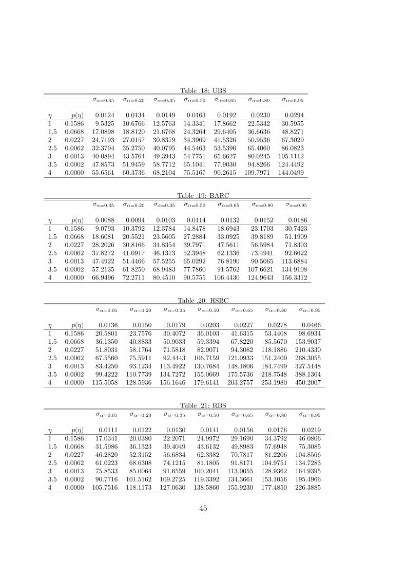
Table .18: UBSσα=0.05 σα=0.20 σα=0.35 σα=0.50 σα=0.65 σα=0.80 σα=0.95

η p(η) 0.0124 0.0134 0.0149 0.0163 0.0192 0.0230 0.02941 0.1586 9.5325 10.6766 12.5763 14.3341 17.8662 22.5342 30.59551.5 0.0668 17.0898 18.8120 21.6768 24.3264 29.6405 36.6636 48.82712 0.0227 24.7193 27.0157 30.8379 34.3969 41.5326 50.9536 67.30292.5 0.0062 32.3794 35.2750 40.0795 44.5463 53.5396 65.4060 86.08233 0.0013 40.0894 43.5764 49.3943 54.7751 65.6627 80.0245 105.11123.5 0.0002 47.8573 51.9459 58.7712 65.1041 77.9030 94.8266 124.44924 0.0000 55.6561 60.3736 68.2104 75.5167 90.2615 109.7971 144.0499

Table .19: BARCσα=0.05 σα=0.20 σα=0.35 σα=0.50 σα=0.65 σα=0.80 σα=0.95

η p(η) 0.0088 0.0094 0.0103 0.0114 0.0132 0.0152 0.01861 0.1586 9.0793 10.3792 12.3784 14.8478 18.6943 23.1703 30.74231.5 0.0668 18.6081 20.5521 23.5605 27.2884 33.0925 39.8189 51.19092 0.0227 28.2026 30.8166 34.8354 39.7971 47.5611 56.5984 71.83032.5 0.0062 37.8272 41.0917 46.1373 52.3948 62.1336 73.4941 92.66223 0.0013 47.4922 51.4466 57.5255 65.0292 76.8190 90.5065 113.68843.5 0.0002 57.2135 61.8250 68.9483 77.7860 91.5762 107.6621 134.91084 0.0000 66.9496 72.2711 80.4510 90.5755 106.4430 124.9643 156.3312

Table .20: HSBCσα=0.05 σα=0.20 σα=0.35 σα=0.50 σα=0.65 σα=0.80 σα=0.95

η p(η) 0.0136 0.0150 0.0179 0.0203 0.0227 0.0278 0.04661 0.1586 20.5801 23.7576 30.4072 36.0103 41.6315 53.4408 98.69341.5 0.0668 36.1350 40.8833 50.9033 59.3394 67.8220 85.5670 153.90372 0.0227 51.8031 58.1764 71.5818 82.9071 94.3082 118.1886 210.43302.5 0.0062 67.5560 75.5911 92.4443 106.7159 121.0933 151.2409 268.30553 0.0013 83.4250 93.1234 113.4922 130.7684 148.1806 184.7499 327.51483.5 0.0002 99.4222 110.7739 134.7272 155.0669 175.5736 218.7548 388.13644 0.0000 115.5058 128.5936 156.1646 179.6141 203.2757 253.1980 450.2007

Table .21: RBSσα=0.05 σα=0.20 σα=0.35 σα=0.50 σα=0.65 σα=0.80 σα=0.95

η p(η) 0.0111 0.0122 0.0130 0.0141 0.0156 0.0176 0.02191 0.1586 17.0341 20.0380 22.2071 24.9972 29.1690 34.3792 46.08061.5 0.0668 31.5986 36.1323 39.4049 43.6132 49.8983 57.6948 75.30852 0.0227 46.2820 52.3152 56.6834 62.3382 70.7817 81.2206 104.85662.5 0.0062 61.0223 68.6308 74.1215 81.1805 91.8171 104.9751 134.72833 0.0013 75.8533 85.0064 91.6559 100.2041 113.0055 128.9362 164.93953.5 0.0002 90.7716 101.5162 109.2725 119.3392 134.3661 153.1056 195.49664 0.0000 105.7516 118.1173 127.0630 138.5860 155.9230 177.4850 226.3885

45