Credit Default Swap Valuation withCounterparty Risk

Seng Yuen Leung1

HSBCHong Kong, China

Yue Kuen Kwok2

Department of MathematicsHong Kong University of Science and Technology

Clear Water Bay, Hong Kong, China

Using the reduced form framework with inter-dependent default correla-tion, we perform valuation of credit default swap with counterparty risk.The inter-dependent default risk structure between the protection buyer,protection seller and the reference entity in a credit default swap are char-acterized by their correlated default intensities, where the default intensityof one party increases when the default of another party occurs. We ex-plore how settlement risk and replacement cost affect the swap rate incredit default swaps.

KEY WORDS: Counterparty risk, contagious defaults, intensity model, credit

default swap

1 Introduction

According to the Credit Derivatives Report of British Bankers’ Association(2002), nearly half of the market share of credit derivatives trading is cap-tured by single-named credit swap contracts. A credit default swap (CDS)is a contract agreement which allows the transfer of credit risk of a riskyasset/basket of risky assets from one party to the other. A financial institu-tion may use a CDS to transfer credit risk of a risky asset while continuesto retain the legal ownership of the asset.3 The rapid growth of the credit

1The opinions expressed in this paper are exclusively the personal views of the authorand should not be cited as opinion and interpretation of HSBC, Hong Kong, China

2Author to whom any correspondence should be addressed. E-mail: maykwok@ust.hk3Apart from hedging purpose, CDSs are recently often used by synthetic deal managers

to tailor credit risk and create arbitrage opportunity not available in the cash markets.

1

default swap market has reached to the stage where credit default swaps onreference entities are more actively traded than bonds issued by the referenceentities. The choice of credit sensitive instruments for empirical studies ondefault risk has slowly moved from risky corporate bonds to credit defaultswaps on the bonds (Longstaff et al . 2003; Ericsson et al ., 2004). Defaultswap premia are believed to reflect changes in credit risk more accuratelyand quickly than corporate bond yield spreads.

Assume that party A holds a corporate bond and faces the credit riskarising from default of the bond issuer (reference party C). To seek protec-tion against such default risk, party A enters a CDS contract in which heagrees to make a stream of periodic premium payments, known as the swappremium to party B (CDS protection seller). In exchange, party B promisesto compensate A (CDS protection buyer) for its loss in the event of default ofthe bond (reference asset). A CDS involves three parties: protection buyer,protection seller, and issuer of the reference bond. Unlike interest rate swapsand currency swaps, where cash flows are exchanged between the two coun-terparties periodically, the protection seller pays only when default of thereference bond occurs.

As remarked by Jarrow and Yu (2001), “an investigation of counterpartyrisk is incomplete without studying its impact on the pricing of credit deriva-tives.” We would like to address the following queries in this paper. How doesthe inter-dependent default risk structure between the protection seller andthe reference bond affect the swap rate? Should we go to a European bank ora Korean bank as the protection seller for a Korean bond? Can the protec-tion seller fulfill its obligation to make the compensation payment at the endof the settlement period, given that its credit quality may have deteriorateddue to contagious effect arising from the default of the reference bond? Whatwould be the impact on the swap rate due to potential replacement cost ofentering a new CDS contract when the protection seller defaults prior to thereference bond? To determine a fair swap rate of a CDS in the presence ofcounterparty risks, the inter-dependent default risk structures between theseparties must be considered simultaneously.

For interest rate swaps, theoretical analyzes show that the difference inswap rates between two counterparties of different credit ratings is much lessthan the difference in their debt rates. For example, for a 5-year interest rateswap between a given party paying LIBOR and another party paying a fixedrate, Duffie and Huang (1996) find that the replacement of the given fixed-rate counterparty with a lower quality counterparty whose bond yields are

2

100 basis points higher would only increase the swap rate by roughly 1 basispoint. However, the very nature of contingent compensation payment upondefault in a CDS may lead to a higher counterparty risk exposure comparedto that of an interest rate swap. Our results show that CDS dealers shouldnot quote the same rates to all counterparties irrespective of their creditratings, like the usual practice in interest rate swaps market.

There have been numerous works on credit default swap valuation. Duffie(1999) proposes a non-model based pricing approach where a credit defaultswap is priced by reference to spreads over the riskfree rate of par floatingrate bonds of the same quality. He also discusses the estimation of the haz-ard rate from defaultable bond prices. Based on the reduced form approachwith correlated market and credit risks, Jarrow and Yildirim (2002) obtainclosed form valuation formula for the swap rate of a CDS. In their model, thedefault intensity is assumed to be “almost” linear in the short interest rate.To examine the impact of counterparty risk on the pricing of a CDS, Jarrowand Yu (2001) assume an inter-dependent default structure that avoids loop-ing default and simplifies the payoff structure where the protection seller’scompensation is made only at the maturity of the swap. They discover thata CDS may be significantly overpriced if the default correlation between theprotection seller and reference entity is ignored. Hull and White (2001) applythe credit index model for valuing CDS with counterparty risk. They arguethat if the default correlation between the protection seller and the referenceentity is positive, then the default of the counterparty will result in a positivereplacement cost for the protection buyer. Their results show that the CDSswap rates increase with credit index correlation and the rates may differ bymore than 10% when the protection seller’s credit rating decreases from AAAto BBB and the value of the credit index correlation is 0.6 or higher. Usinga structural default correlation model, Kim and Kim (2003) conclude thatthe pricing error in a CDS can be quite substantial if the correlation betweenthe default risks of the counterparty and reference bond is ignored. Chenand Filpovic (2003) develop a generalized affine model to price credit defaultswaps under default correlations and counterparty risk. By the specificationanalysis of the affine process, they manage to incorporate market-credit riskcorrelation, joint credit migrations and firm specific default risk into theirpricing model. Yu (2004) uses the “total hazard” approach to construct thedefault processes from independent and identically distributed exponentialrandom variables. He obtains an analytic expression of the joint distributionof default times in his two-firm and three-firm contagion models. Under the

3

framework of contagious defaults, the default risk is modeled by the reducedform approach, where the probability of default is determined by an exoge-nously specified instantaneous default intensity. The contagious defaults areeffected by inter-dependent default risk structure between the parties, wherethe default intensity of one party increases when the default of another partyoccurs.

In this paper, we would like to analyze the impact of correlated risksbetween the three parties in a CDS using similar contagion models. Insteadof following Yu’s approach, we employ the change of measure introducedby Collins-Dufresne et al . (2002) in our valuation procedures. Using thischange of measure, our counterparty risk model reduces to the standardreduced form model. Specifically, the probability measure of firm i is definedby its default intensity which is absolutely continuous with respect to the riskneutral measure and zero probability is assigned to firm i if default occursbefore maturity. Compared to the total hazard construction (Yu, 2004), theanalytic derivation procedures using the change of measure approach becomeless tedious. In his CDS pricing model, Yu (2004) places several assumptionson the payment structures in order to simplify his calculations. Firstly, theprotection buyer is assumed to make continuous premium payment at theswap rate till expiration, provided that the buyer does not default prior toexpiry. However, the swap payment terminates upon default of either oneof the three parties in market practice. Secondly, the protection seller isassumed to make the contingent compensation payment on the expirationdate, provided that the protection seller survives beyond the expiration dateof the swap.

Distinctive from others’ work on CDS valuation with counterparty risk,we consider the more realistic scenario in which the compensation paymentupon default of the reference party is made at the end of the settlementperiod after default. If the protection seller defaults prior to the referenceentity, then the protection buyer renews the CDS with a new counterparty.Supposing that the default risks of the protection seller and reference entityare positively correlated, we would like to estimate the expected replacementcost due to an increase in the swap rate in the new CDS. The change ofmeasure technique provides an effective tool for CDS valuation in our morerefined pricing model. Furthermore, we extend our counterparty risk frame-work to the three-firm contagion model by including the possibility of defaultof the protection buyer. This represents an extension from unilateral defaultto bilateral defaults among the counterparties.

4

The paper is organized as follows. In Section 2, we present the setupof the two-firm contagion model. We employ the inter-dependent defaultmodel to analyze the effects of settlement risk and replacement cost on thefair swap rate of a CDS. In Section 3, the analysis of correlated default risksin CDS valuation is extended to the three-firm model where all three partieshave inter-dependent default structure. The paper is ended with conclusiveremarks in the last section.

2 Two-firm Model

We consider an uncertain economy with a time horizon of T described by afiltered probability space (Ω,F , FtT

t=0, P ) satisfying F = FT , where P isthe risk-neutral (equivalent martingale) measure in the sense of Harrison andKreps (1979), that is, all security prices discounted by the risk-free interestrate process rt are martingale under P . We use the Cox framework to specifythe random default times. We denote the default time of firm i by

τ i = inf

t :

∫ t

0

λis ds ≥ Ei

, (1a)

where Eii∈I is a set of independent unit exponential random variables. Wefurther assume that τ i possesses a strictly positive Ft-predictable intensityλi

t with right-continuous sample paths such that

M it = Nt −

∫ t∧τ i

0

λis ds (1b)

is a (P,Ft)-martingale. Under the above characterization, given the FXt -

adapted intensity λit, the conditional survival probability of firm i is given

by

P [τ i > T |Ft] = E

[exp

(−

∫ T

t

λis ds

)∣∣∣Ft

]. (2)

In this section, we perform credit default swap valuation using the two-firm contagion model. The likelihood of default of the protection seller (firmB) with random default time τB and the reference entity (firm C) with ran-dom default time τC are modeled by their correlated default intensities whilethe protection buyer (firm A) is assumed to be default-free. Under the CDScontract, a periodic stream of swap premium payments will be paid to the

5

protection seller until the occurrence of a contractually defined credit event(either protection seller defaults or the reference entity defaults) or the expi-ration of the contract, whichever comes earlier. If the reference entity defaultsprior to the expiration of the contract, then the protection buyer receives thecompensation from the protection seller on the settlement date (at the endof the settlement period). The compensation is given by the difference be-tween the face value and the recovery value of the reference entity, less theswap premium that has accrued since the last payment date. The accruedpremium is calculated on a time-proportional basis. If the protection sellerdefaults prior to the default of the reference entity, the contract terminates.The protection buyer enters a new contract with another counterparty forthe remaining life of the original CDS.

To simplify our CDS valuation, we assume a flat term structure of risklessinterest rate r.4 In our two-firm contagion model, the inter-dependent defaultrisk structure between firm B and firm C is characterized by the correlateddefault intensities:

λBt = b0 + b21τC≤t (3a)

λCt = c0 + c21τB≤t, (3b)

where the default intensity λBt (λC

t ) jumps by the amount b2 (c2) when firmC (B) defaults. The parameters b0, b2, c0 and c2 are assumed to be constantand distinct. Without loss of generality, we take the notional to be $1 andassume zero recovery upon default. Since it takes no cost to enter a CDS,the value of the swap rate S2(T ) under this two-firm model is determined by

n∑

i=1

E[e−rTi S2(T ) 1τB∧τC>Ti

]+ S2(T )A2(T )

= E[e−r(τC+δ)1τC≤T1τB>τC+δ

], (4)

where T1, · · · , Tn are the swap payment dates with 0 = T0 < T1 < · · · <Tn = T and δ is the length of the settlement period. Here, τC + δ representsthe settlement date at the end of the settlement period. We assume thatthe payment dates are uniformly distributed, that is, Ti+1 − Ti = ∆T for1 ≤ i ≤ n − 1. The first term in Eq. (4) gives the present value of the sum

4Without loss of analytical tractability, our framework can be extended to stochasticinterest rate within the class of affine structure.

6

of periodic swap payments (terminated when either B or C defaults or atmaturity) and S2(T )A2(T ) is the present value of the accrued swap premiumfor the fraction of period between τC and the last payment date. The presentvalue of accrued swap premium is given by

S2(T )A2(T ) = S2(T )

n∑

i=1

E

[e−rτC

(τC − Ti−1

∆T

)1Ti−1<τC<Ti1τB>τC

], (5)

where the accrued premium is paid at τC andτC − Ti−1

∆Trepresents the frac-

tion of the time interval between successive payment dates. To computeS2(T ), we set the present value of protection buyer’s payment equal to thepresent value of the compensation payment made at τC + δ, conditional ondefault of C prior to T and no default of B prior to τC + δ. The buyer mayface potential replacement cost when τB < min(τC, T ). However, since S2(T )represents the fair swap rate charged by the seller party B, the replacementcost should not be included in the calculation of the swap premium.

Compared to other CDS valuation models in the literature, our pricingframework models the payoff structures closer to reality, in particular, thecompensation is payable in the end of settlement period after C’s default,and periodic discrete payments are made at T1, . . . , Tn.

2.1 Change of Measure

We adopt the change of measure introduced by Collins-Dufresne et al . (2002)in our valuation procedure of the swap rate. Accordingly, we define a firm-specific probability measure P i which puts zero probability on the pathswhere default occurs prior to the maturity T . Specifically, the change ofmeasure is defined by

ZT ,dP i

dP

∣∣∣∣∣FT

= 1τ i>T exp

(∫ T

0

λis ds

), (6)

where P i is a firm-specific (firm i) probability measure which is absolutelycontinuous with respect to P on the stochastic interval [0, τ i). One can showthat ZT is a uniformly integrable P -martingale with respect to FT and isalmost surely strictly positive on [0, τ i) and almost surely equal to zero on[τ i,∞) [see Collins-Dufresne et al . (2004)]. To proceed the calculations under

7

the measure P i, we enlarge the filtration to F i = (F it )t≥0 as the completion

of F = (Ft)t≥0 by the null sets of the probability measure P i.Under the default risk structure specified in Eq. (3a,b), the survival prob-

abilities of firm B and firm C are defined recursively through each other andthis leads to the phenomenon of “looping default.” Under the new measureP B defined by Eq. (6), λC

t = c0 for t < T , so this effectively neglect theimpact of firm B’s default on the intensity of firm C, so looping default nolonger exists. An analogous argument also holds under the measure P C.

Using the change of measure, the joint density of default times (τB, τC)is found to be (see Appendix A)

f(t1, t2) =

c0(b0 + b2)e

−(b0+b2)t1−(c0−b2)t2, t2 ≤ t1,

b0(c0 + c2)e−(c0+c2)t2−(b0−c2)t1, t2 > t1.

(7)

The marginal density of the default times τB and τC can be obtained byintegrating the joint density f(t1, t2). This gives

P [τB ∈ dt1]

dt1=

(b0 + b2)c0

c0 − b2

[e−(b0+b2)t1 − e−(b0+c0)t1

]+ b0e

−(b0+c0)t1 (8a)

and

P [τC ∈ dt2]

dt2=

(c0 + c2)b0

b0 − c2

[e−(c0+c2)t2 − e−(b0+c0)t2

]+ c0e

−(b0+c0)t2. (8b)

Consequently, the marginal survival probabilities are given by

P [τB > t1] =c0e

−(b0+b2)t1 − b2e−(b0+c0)t1

c0 − b2

, (9a)

and

P [τC > t2] =b0e

−(c0+c2)t2 − c2e−(b0+c0)t2

b0 − c2. (9b)

2.2 Swap Premium in the Two-firm Model

Using the joint density f(t1, t2) given in Eq. (7) and performing the expec-tation calculations in Eq. (4), one can show that the swap premium is givenby (see Appendix B)

S2(T ) =c0e

−(b0+b2+r)δ(1 − e−βT )

β

[e−β∆T (1 − e−βn∆T )

1 − e−β∆T+ A2(T )

]−1

, (10)

8

where β = b0+c0+r and the expression for A2(T ) is given in Appendix B. It isinteresting to observe that S2(T ) is independent of c2, though the calculationof S2(T ) involves E[e−rTi1τB∧τC>Ti]. A more careful consideration revealsthat an increase of the default intensity of C by c2 due to B’s default wouldhave impact only on the replacement cost. Since the calculation of S2(T )does not include the effect of replacement cost, the independence of S2(T )on c2 seems logically.

The impact of contagious default structure between the protection sellerB and the reference asset C on the swap premium is illustrated in Figure 1.Consistent with our intuition, the swap premium decreases with b0 as theprotection buyer is willing to pay a lower premium when dealing with a morerisky protection seller. The swap premium becomes smaller as b2 assumes ahigher value because the default of C increases the default probability of B.Similar to other credit risk factors, the swap premium is highly sensitive tothe underlying default risk of C proxied by c0.

From Eq. (10), one deduces that the swap premium is not quite sensitiveto the length of the protection period. This is consistent with the empiricalstudies by Aunon-Nerin et al . (2002). They have tested several specificationsfor the maturity effect, but none of them appear to be significant.

2.3 Settlement Risk and Replacement Cost

We now turn our attention to the settlement risk and replacement cost in aCDS. Suppose a financial institution enters a CDS to protect its underlyingasset. But this does not mean that default risk can be fully hedged due tothe possibility of swap seller’s default occurred before the settlement date.Observe that if firm B is default-free, the swap premium is then given by

n∑

i=1

E[e−rTiS2(T ) 1τC>Ti

]+ S2(T )A2(T ) = E

[e−r(τC+δ)1τC≤T

], (11)

where

A2(T ) =n∑

i=1

E

[e−rτC

(τC − Ti−1

∆T

)1Ti−1<τC<Ti

].

To examine the effect of settlement risk on the swap premium , we define theswap premium spread V (T ) to be the difference of the swap premium with

9

and without settlement risk, that is,

V (T ) = S2(T )− S2(T ). (12)

Intuitively speaking, it is not clear that whether V (T ) is strictly positive.In a CDS, the protection buyer inevitably faces a trade-off between a higherpresent value of compensation for its loss in the event of C’s default, that is,

E[e−r(τC+δ)1τC≤T

]≥ E

[e−r(τC+δ)1τC≤T1τB>τC+δ

]

and a higher present value of total swap payments due to an obligation tomake compensation to swap buyer upon the default of underlying asset, thatis,

E[e−rTi1τC>Ti

]+ A2(T ) ≥ E

[e−rTi1τB∧τC>Ti

]+ A2(T ).

It is quite straightforward to derive S2(T ), which can be obtained by settingb0 = b2 = 0 in S2(T ).

The change on settlement risk premium with respect to the settlementperiod δ is illustrated in Figure 2. We observe that the settlement riskpremium increases as δ becomes larger, and its sensitivity is very significant.Doubling the value of c0 from 0.1 to 0.2 leads to a significant increase of60 basis points in the settlement risk premium. The effect of b0 and b2

have relatively less influence on the settlement risk premium. We find thatthe default correlation between the protection seller and the reference asset,proxied by b2, is slightly more important than the underlying risk of theprotection seller when settlement risk is analyzed. This suggests that theprotection buyer should be aware of the credit rating of its counterparty B,its correlated default risk with the reference asset as well as the settlementperiod in order to determine a fair swap premium.

From protection buyer’s perspective, it is uncertain to pay a stream offixed payments for credit protection throughout the whole period due to thedefault of the protection seller. In the presence of counterparty risk, the creditrating of the reference entity varies over time. This results a change in swappremium when entering a CDS at a different time. Specifically, the protectionbuyer can benefit or lose from a new contact, depending upon the creditrating of the reference entity at the default time of the original protectionseller. In our model, the rating movement depends on the sign of b2 and c2.We define the replacement cost as the excess premium required to enter a newcontract upon the default of the original protection seller. Mathematically,

10

the default intensity of the reference entity becomes a constant after thedefault of the protection seller, that is,

λCt = c0 + c2. (13)

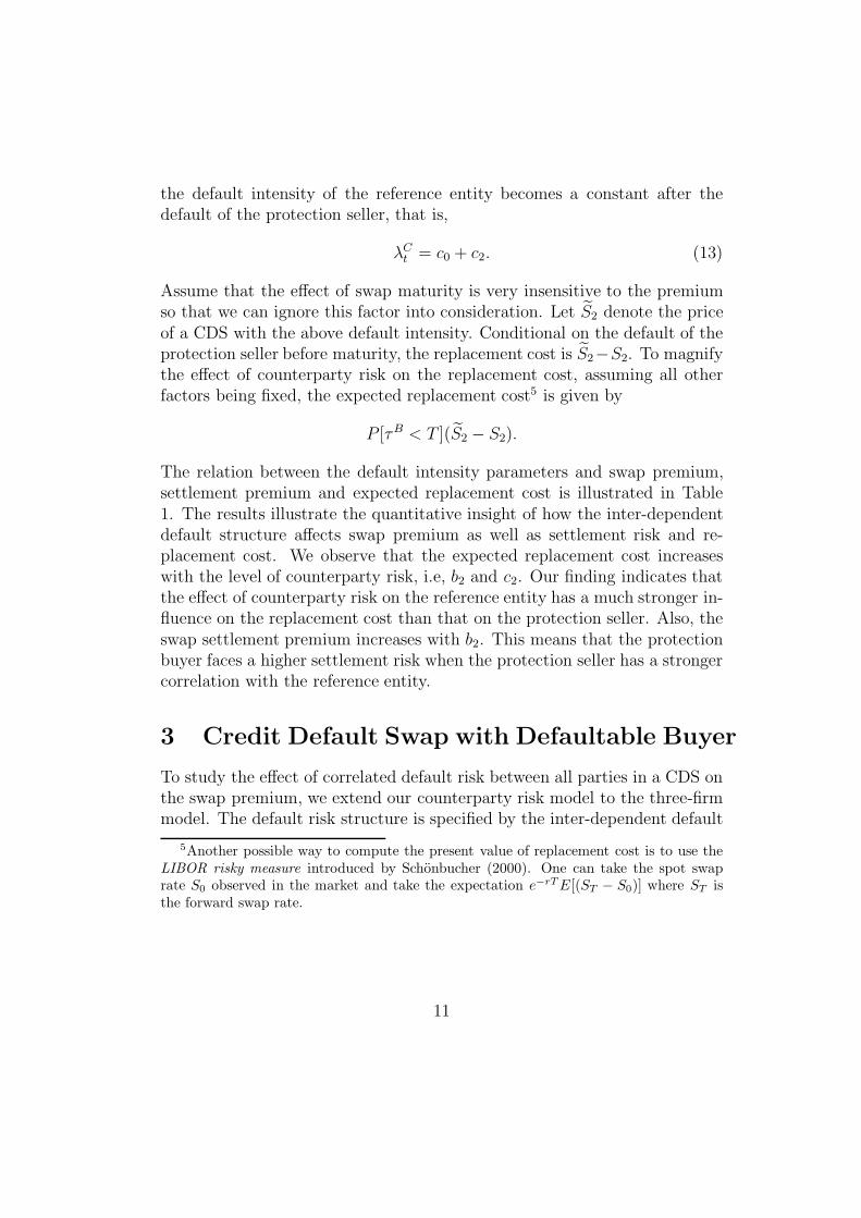
Assume that the effect of swap maturity is very insensitive to the premiumso that we can ignore this factor into consideration. Let S2 denote the priceof a CDS with the above default intensity. Conditional on the default of theprotection seller before maturity, the replacement cost is S2−S2. To magnifythe effect of counterparty risk on the replacement cost, assuming all otherfactors being fixed, the expected replacement cost5 is given by

P [τB < T ](S2 − S2).

The relation between the default intensity parameters and swap premium,settlement premium and expected replacement cost is illustrated in Table1. The results illustrate the quantitative insight of how the inter-dependentdefault structure affects swap premium as well as settlement risk and re-placement cost. We observe that the expected replacement cost increaseswith the level of counterparty risk, i.e, b2 and c2. Our finding indicates thatthe effect of counterparty risk on the reference entity has a much stronger in-fluence on the replacement cost than that on the protection seller. Also, theswap settlement premium increases with b2. This means that the protectionbuyer faces a higher settlement risk when the protection seller has a strongercorrelation with the reference entity.

3 Credit Default Swap with Defaultable Buyer

To study the effect of correlated default risk between all parties in a CDS onthe swap premium, we extend our counterparty risk model to the three-firmmodel. The default risk structure is specified by the inter-dependent default

5Another possible way to compute the present value of replacement cost is to use theLIBOR risky measure introduced by Schonbucher (2000). One can take the spot swaprate S0 observed in the market and take the expectation e−rT E[(ST − S0)] where ST isthe forward swap rate.

11

intensities

λAt = a0 + a11τB≤t + a21τC≤t, (14a)

λBt = b0 + b11τA≤t + b21τC≤t, (14b)

λCt = c0 + c11τA≤t + c21τB≤t. (14c)

From this setting, it is evident that the default probability of each partyin the CDS depends on the default status of other firms. This model nestsa number of simpler models. For instance, it reduces to the two-firm modelin Section 2 if we take a0 = a1 = a2 = 0. If we take c1 = c2 = 0, the defaultstatus of both counterparties in the CDS do not affect the credit rating of thereference asset. One may provide the financial interpretation as follows: thereference asset, say a risky bond, is issued by a large firm C whose defaulthas an economy-wide impact. A small firm A holds this bond and wants toenter a CDS for the protection of the bond upon C’s default. Suppose thatA finds a swap seller, say B, in the same sector, so A and B have correlateddefault risk.

3.1 Swap Premium in the Three-firm Model

We employ the three-firm model specified by Eqs.(6a,6b,6c) to price a CDS.Under this framework, we study the effect of each party’s default on the swappremium. Suppose that the protection buyer (firm A) holds a defaultableasset issued by firm C, and enter a CDS contract from the protection seller(firm B). Distinct from the two-firm model, the protection buyer is obligatedto pay the periodic swap premium until the expiration of the contract, or theoccurrence of the default either by the protection seller, the reference asset oritself, whichever is earlier. As before, upon the default of the reference asset,the protection buyer receives from the protection seller the difference betweenthe face value and the recovery value of the reference entity. Moreover,if the protection buyer defaults prior to the default of the reference asset,the protection seller can simply walk away from the contract and has noobligation to pay the compensation to the protection seller.

In the presence of defaultable swap buyer, the swap premium is deter-

12

mined by

n∑

i=1

E[e−rTiS3(T )1τA∧τB∧τC>Ti

]+ S3(T )A3(T )

= E[e−r(τC+δ)1τC≤T1τA>τC1τB>τC+δ

]. (15)

To determine the swap premium S3(T ), it requires the knowledge of thejoint density f(t1, t2, t3) of (τA, τB, τC). By following similar calculation pro-cedures as those for the two-firm model, the joint density f(t1, t2, t3) is foundto be

f(t1, t2, t3) =

a0(b0 + b1)(c0 + c1 + c2)×e−(a0−b1−c1)t1−(b0+b1−c2)t2−(c0+c1+c2)t3, t1 < t2 < t3,a0(c0 + c1)(b0 + b1 + b2)×e−(a0−b1−c1)t1−(c0+c1−b2)t3−(b0+b1+b2)t2, t1 < t3 < t2,b0(a0 + a1)(c0 + c1 + c2)×e−(b0−a1−c2)t2−(a0+a1−c1)t1−(c0+c1+c2)t3, t2 < t1 < t3,c0(a0 + a2)(b0 + b1 + b2)×e−(c0−a2−b2)t3−(a0+a2−b1)t1−(b0+b1+b2)t2, t3 < t1 < t2,b0(c0 + c2)(a0 + a1 + a2)×e−(b0−c2−a1)t2−(c0+c2−a2)t3−(a0+a1+a2)t1, t2 < t3 < t1,c0(b0 + b2)(a0 + a1 + a2)×e−(c0−b2−a2)t3−(b0+b2−a1)t2−(a0+a1+a2)t1, t3 < t2 < t1.

(16)With the aid of f(t1, t2, t3), the swap premium S3(T ) is given by

S3(T ) = Lχ(T )

[e−α∆T (1 − e−αn∆T )

1 − e−α∆T+ A3(T )

]−1

e−rδ, (17)

where α = a0 + b0 + c0 + r, Lχ(T ) and A3(T ) are presented in Appendix D.Note that when we set a0 = a1 = a2 = 0, S3(T ) reduces to the swap premiumS2(T ) in Eq. (10).

In Figures 3 and 4, we plot the swap premium against varying values ofdefault intensity parameters in the three-form model. Figure 3 illustratesthat the reference asset’s default risk proxied by c0 gives the most significantimpact on swap premium, and an increasing higher value of c0 gives rise to ahigher swap premium. On the other hand, the default risk of the protectionbuyer has little impact on the swap premium, i.e., an increase in the likeli-hood of default of the protection buyer (a higher value of a0) only increases

13

the swap premium marginally. It is because when the financial health of theprotection seller affects the default status of the underlying asset, this con-tagion effect makes the underlying asset more risky, in turn the protectionseller would take a higher swap premium. Unlike the effect of the protectionseller and the underlying asset, this effect is of third-order, so the impact ismuch less significant.

The expression for the swap premium in Eq. (17) shows no dependenceon a1, c1, and c2. Financially speaking, prior to the default of the underlyingasset, the default event of the protection buyer or the protection seller willterminate the contract. This explains why a1, c1 and c2 have no influenceon the swap premium. Though S3(T ) in Eq. (17) has dependence on a2,one can show that the change of the swap premium is insensitive to a2, andthis can be explained by a similar argument. Figure 4 illustrates the changeof swap premium with respect to varying levels of the default risk of theprotection seller. The swap premium declines with the credit quality of theprotection seller proxied by b0. However, the degree of magnitude in thechange is relatively low compared with that of c0. In addition, a strongercorrelated default risk with other counterparties on the protection seller, alower swap premium the protection buyer is willing to pay, as seen by theincreases in b1 and b2 lead to lower swap premium, while the swap premium ismore sensitive to b2. The order of sensitivity to the protection seller is b2, b0

and b1. Similar to the two-firm model, the swap premium is also insensitiveto maturity.

4 Conclusion

In this paper, using both the two-firm and three-firm contagion risk models,we provide the insight on how counterparty risks influence the swap rate ina credit default swap. It may be possible for a financial institution to havegood estimates of marginal distributions (or default intensities), yet end upwith the wrong evaluation of its credit exposure. For example, firm A couldestimate a parametric model using the bond prices issued by firm B. However,if the counterparty risk for firm B is incorrectly identified by another partywhose default is independent of firm C, this could severely overprice the swaprate due to neglect of default correlation. Our findings can be summarizedas follows:

1. For CDS valuation, the swap premium can be significantly affected by

14

counterparty risk. If the protection seller (firm B) has a higher correla-tion with the reference asset (firm C), then the swap premium becomesslightly lower. It is due to the fact that the swap buyer (firm A) is ex-pected to pay a lower swap premium for less protection on its referenceasset. On the other hand, when C has a higher correlation with A andB, the swap premium has no change at all. Though the occurrence ofdefault either of A or B (prior to the default of C) increases the defaultprobablility of C, the contract is then immediately terminated, so ithas no impact on the swap premium. The same reasoning can be usedto explain the insignificant change on the swap premium due to the im-pact of A’s default on B. Due to the very nature of the CDS structure,the impact of default either of B or C on A does not give any changeon the swap premium. Suppose B defaults prior to C, A can simplywalk away and enter a new contract for the remaining period. WhenA survives longer than C during the life of the contract, A will receivecompensation from B, independent of whether A defaults or not beforethe settlement date. In summary, the default risk of C is the primarydeterminant of the swap premium, and a higher value of c0 leads to asignificant increase in swap premium. Both results agree with finan-cial intuition. Furthermore, the swap premium increases with a0 anddeclines with b0, but this effect is comparatively less pronounced.

2. The swap premium shows almost a flat term structure for all maturities.This behavior is probably attributed to our CDS payment structure.When B defaults prior to C’s default, the protection buyer can simplywalk away and enters a new contract for the remaining period. How-ever, when the protection buyer defaults prior to C’s default, B has theright to terminate the contract and has no obligation on the protec-tion. This leads to the insensitivity of the swap premium with respectto maturity.

3. The change of settlement risk premium with respect to the settlementperiod is highly sensitive: a longer settlement period, a higher settle-ment risk premium. This suggests that the protection buyer shouldbe aware of the credit rating of its counterparty B and the settlementperiod in order to determine a fair swap premium.

Our work also provides the motivation for investigating other credit riskissues. It is worth to study the effect of counterparty risk on other credit

15

derivatives and structured products. Since the default intensity of one partyjumps until another party defaults, the contagion model is unable to capturethe intermediate change in credit rating of counterparties prior to creditevent. Unlike structural models, it is not appropriate to use our frameworkto price structured credit products with strong dependence on the prior-to-maturity change in credit rating. On the other hand, the contagion modelprovides nice analytic tractability for multi-asset instruments while moststructural models have great difficulty to provide an extension to the inter-dependent default structure for a basket of multiple assets.

References

Aunon-Nerin, D., Cossin, D., Hricko, T., and Huang, Z. (2002). Exploring for the deter-minants of credit risk in credit default swap transaction data: Is fixed-income markets’information sufficient to evaluate credit risk?. Working paper of HEC-University of Lau-sanne and FAME.

British Bankers’ Association (2002). BBA Credit derivatives report 2001/2002.

Chen, L., and Filipovic, D. (2003). Pricing credit default swaps under default correlationsand counterparty risk. Working paper of Princeton University.

Collin-Dufresne, P., Goldstein, R., and Hugonnier, J. (2002). A general formula for pricingdefaultable securities. Econometrica 72, 1377-1407.

Duffie, D., and Huang, M. (1996). Swap rate and credit quality, Journal of Finance 51,921-949.

Duffie, D. (1999). Credit swap valuation. Financial Analysts Journal Jan/Feb issue,73-87.

Ericsson, J., Jacobs, K., and Oviedo-Helfenberger, R. (2004). The determinants of creditdefault swap premia. Working paper of McGill University.

Harrison, M., and Kreps, D. (1979). Martingales and arbitrage in multi-period securitiesmarkets. Journal of Economic Theory 20, 381-408.

Hull, J., and White, A. (2001). Valuing credit default swaps II: modeling default correla-tions. Journal of Derivatives 8, 12-22.

16

Jarrow, R., and Yu, F. (2001). Counterparty risk and the pricing of defaultable securities.Journal of Finance 56, 1765-1799.

Jarrow, R., and Yildirim, Y. (2002). A simple model for valuing default swaps when bothmarket and credit risk are correlated. Journal of Fixed Income 11(4), 7-19.

Kim, M.A., and Kim, T.S. (2003). Credit default swap valuation with counterparty defaultrisk and market risk. Journal of Risk 6(2), 49-80.

Longstaff, F.A., Mithal, S., and Neis, E. (2003). The credit-default swap market: Is creditprotection priced correctly. Working paper of University of California at Los Angeles.

Schonbucher, P. (2000). A LIBOR market model with default risk. Working paper ofBonn University.

Yu, F. (2004). Correlated defaults and the valuation of defaultable securities. Workingpaper of University of California at Irvine.

17

Appendix

A. Joint density of default times (τB, τC)

Let EC[·] denote the expectation taken under the measure P C . Fort1 < t2, the joint distribution of the pair of default times is found to be

P [τB > t1, τC > t2]

= E[1τB>t11τC>t2

]

= EC

[1τB>t1 exp

(−

∫ t2

0

(c0 + c21τB≤s) ds

)]

= e−c0t2EC[1τB>t1 exp

(−c2(t2 − τB)1τB≤t2

)]

= e−c0t2

[∫ t2

t1

b0e−b0u−c2(t2−u) du +

∫ ∞

t2

b0e−b0u du

]

= b0e−(c0+c2)t2

[e−(b0−c2)t1 − e−(b0−c2)t2

b0 − c2

]+ e−(b0+c0)t2.

The fourth equality follows from the fact that λBt = b0 for t ≤ t2 under P C .

By a similar argument, for t2 < t1, the joint distribution is given by

P [τB > t1, τC > t2] = c0e

−(b0+b2)t1

[e−(c0−b2)t2 − e−(c0−b2)t1

c0 − b2

]+ e−(b0+c0)t1.

The differentiation of P [τB > t1, τC > t2] with respect to t1 and t2 gives the

joint density of the default times in Eq. (7).

B. Swap premium S2(T ) of the two-firm model

Using the joint density f(t1, t2), we obtain

E

[e−

∫ τC+δ0 r ds1τC≤T1τB>τC+δ

]=

c0e−(b0+b2+r)δ[1 − e−(b0+c0+r)T ]

b0 + c0 + r.

To evaluate E[e−rTi1τB∧τC>Ti

], we can take the advantage of the change

of measure to avoid tedious integration involving f(t1, t2). Specifically, wehave

18

E[e−rTi1τB∧τC>Ti

]

= e−rTiE[1τB>Ti1τC>Ti

]

= e−rTiEC

[1τB>Ti exp

(−

∫ Ti

0

(c0 + c2)1τB≤s ds

)]

= e−(c0+r)TiEC[1τB>Ti

]

= e−(b0+c0+r)Ti.

By letting β = b0 + c0 + r and observing ∆T = Ti+1 − Ti for 1 ≤ i ≤ n − 1,we obtain

n∑

i=1

e−(b0+c0+r)Ti =e−β∆T (1 − e−βn∆T )

1 − e−β∆T.

In Appendix D, we will derive A3(T ). Since A3(T ) is an extension of A2(T )with the inclusion of the default possibility of the protection buyer, A3(T ) isreduced to A2(T ) by taking a0 = 0. Combining all these results, we obtainthe swap premium S2(T ) in Eq. (10). As a result, we obtain

A2(T ) =c0

∆T

[1 − e−(b0+c0+r)T

(b0 + c0 + r)2− Te−(b0+c0+r)T

b0 + c0 + r

]

− c0

b0 + c0 + r

N∑

i=1

Ti−1

[e−(b0+c0+r)Ti−1 − e−(b0+c0+r)Ti

].

C. Joint density of default times (τA, τB, τC)

Suppose t1 < t2 < t3, we have

P [τA > t1, τB > t2, τ

C > t3]

= E[1τA>t11τB>t21τC>t3

]

= EC

[1τA>t11τB>t2 exp

(−

∫ t3

0

(c0 + c11τA≤s + c21τB≤s) ds

)]

= e−c0t3EC[1τA>t11τB>t2 e

−c1(t3−τA) 1τA≤t3−c2(t3−τB) 1τB≤t3

].

19

Note that

1τA>t11τB>t2

= 1t1<τA≤t21t2<τB≤t3 + 1t2<τA≤t31t2<τB≤t3 + 1τA>t31t2<τB≤t3

+1t1<τA≤t21τB>t3 + 1t2<τA≤t31τB>t3 + 1τA>t31τB>t3.

Hence, we have

P [τA > t1, τB > t2, τ

C > t3]

= e−(c0+c1+c2)t3EC[1t1<τA≤t21t2<τB<t3e

c1τA+c2τB]

+ e−(c0+c1+c2)t3EC[1t1<τA≤t21τB>t3e

c1τA]

+ e−(c0+c1+c2)t3EC[1t2<τA≤t31t2<τB≤t3e

c1τA+c2τB]

+ e−(c0+c1+c2)t3EC[1t2<τA≤t31τB>t3e

c1τA]

+ e−(c0+c1+c2)t3EC[1t2<τB≤t31τA>t3e

c2τB]

+ e−(c0+c1+c2)t3EC[1τA>t31τB>t3

].

Under the measure P C and for t < t3, the default intensities λAt and λB

t aregiven by

λAt = a0 + a11τB≤t

λBt = b0 + b11τA≤t.

Using the joint density of (τA, τB)

f(u1, u2) = a0(b0 + b1)e−(b0+b1)u2−(a0−b1)u1 , u1 < u2,

one can compute EC[1t1<τA≤t21τB>t3e

c1τA]

and other similar terms.

Once we have obtained P [τA > t1, τB > t2, τ

C > t3], we differentiate thedistribution function with respect to t1, t2 and t3 to give the joint densityfunction

f(t1, t2, t3) = a0(b0 + b1)(c0 + c1 + c2) e−(a0−b1−c1)t1−(b0+b1−c2)t2−(c0+c1+c2)t3,

for t1 < t2 < t3.

20

We can obtain f(t1, t2, t3) for other permutation in a similar manner and getthe results in Eq. (16).

D. Swap premium S3(T ) of the three-firm model

Using the joint density function f(t1, t2, t3) for t3 < t2 < t1 and t3 <t1 < t2, we obtain

Lχ(T )

, E[e−r(τC+δ)1τC≤T1τA>τC1τB>τC+δ

]

=c0(a0 + a2)e

−(b0+b1+b2+r)δ

(a0 + a2 − b1)(a0 + b0 + c0 + r)

[1 − e−(a0+b0+c0+r)T

]

− c0(a0 + a2)(b0 + b1 + b2)e−(a0+a2+b0+b2+r)δ

(a0 + a2 − b1)(a0 + b0 + c0 + r)(a0 + a2 + b0 + b2)

[1 − e−(a0+b0+c0+r)T

]

+c0(b0 + b2)(b0 + b1 + b2)e

−(a0+a2+b0+b2+r)δ

(a0 + b0 + c0 + r)(a0 + a2 + b0 + b2)

[1 − e−(a0+b0+c0+r)T

]

where the vector of parameters χ = (a0, a2, b0, b1, b2, c0) captures the corre-lated default “characteristic.” The expectation E

[e−rTi1τA∧τB∧τC>Ti

]can

be handled in a similar fashion as that in the two-firm model. The expecta-tion calculations are given by

E[e−rTi1τA∧τB∧τC>Ti

]

= e−rTiEA

[1τB>Ti1τC>Ti exp

(−

∫ Ti

0

(a0 + a1)1τB≤s + a21τC≤s ds

)]

= e−(a0+r)TiEA[1τB>Ti1τC>Ti

].

For t ≤ Ti, the dynamics of the default intensities of firm B and firm C underP A are

λBt = b0 + b21τC≤t

λCt = c0 + c21τB≤t.

Using the result in the two-firm model (see Appendix B), we have

EA[1τB>Ti1τC>Ti

]= e−(b0+c0)Ti,

21

and soE

[e−rTi1τA∧τB∧τC>Ti

]= e−(a0+b0+c0+r)Ti.

This leads to

n∑

i=1

E[e−rTi1τA∧τB∧τC>Ti

]=

e−α∆T (1 − e−αn∆T )

1 − e−α∆T,

where α = a0 + b0 + c0 + r. It remains to evaluate A3(T ), which is defined by

A3(T ) =n∑

i=1

E

[e−rτC

(τC − Ti−1

∆T

)1Ti−1<τC<Ti1τA∧τB>τC

].

Using f(t1, t2, t3) for t3 < t2 < t1 and t3 < t1 < t2, and performing straight-forward integration, we obtain

E[e−rτC

1Ti−1<τC<Ti1τA∧τB>τC

]

=c0

a0 + b0 + c0 + r

[e−(a0+b0+c0+r)Ti−1 − e−(a0+b0+c0+r)Ti

],

and

E[τCe−rτC

1Ti−1<τC<Ti1τA∧τB>τC

]

= c0

[e−(a0+b0+c0+r)Ti−1 − e−(a0+b0+c0+r)Ti

(a0 + b0 + c0 + r)2

+Ti−1e

−(a0+b0+c0+r)Ti−1 − Tie−(a0+b0+c0+r)Ti

a0 + b0 + c0 + r

]

As a result, we obtain

A3(T ) =c0

∆T

[1 − e−(a0+b0+c0+r)T

(a0 + b0 + c0 + r)2− Te−(a0+b0+c0+r)T

a0 + b0 + c0 + r

]− c0

(a0 + b0 + c0 + r)∆Tn∑

i=1

Ti−1

[e−(a0+b0+c0+r)Ti−1 − e−(a0+b0+c0+r)Ti

].

22

(b0, c0)

(b2, c2) (0.05, 0.05) (0.1, 0.05) (0.05, 0.1)1.21% 1.21% 2.44%

(0.05, 0.05) 0.02% 0.03% 0.05%0.59% 0.85% 0.63%1.20% 1.20% 2.41%

(0.1, 0.05) 0.04% 0.05% 0.08%0.62% 0.89% 0.73%1.22% 1.21% 2.44%

(0.05, 0.1) 0.02% 0.03% 0.05%1.12% 1.67% 1.23%

Table 1: The entries illustrate the effect of the underlying defaultrisk (b0 and c0) and the counterparty risk (b2 and c2) onthe swap premium (first row), settlement premium (sec-ond row) and replacement cost (third row). We take thenotional to be $1, risk-free interest rate r to be 5%, matu-rity T of 10 years, and settlement period δ of 0.25 year.

23

0 0.05 0.1 0.15 0.2 0.25 0.3 0.35 0.4 0.45 0.52.15

2.2

2.25

2.3

2.35

2.4

2.45

2.5

2.55

2.6

2.65

b0

Sw

ap P

rem

ium

in P

erce

ntag

e (%

)

b2=0.15, c

0=0.1

b2=0.3, c

0=0.1

b2=0.15, c

0=0.11

0 0.05 0.1 0.15 0.2 0.25 0.3 0.35 0.4 0.45 0.5

2.2

2.4

2.6

2.8

b2

Sw

ap P

rem

ium

in P

erce

ntag

e (%

)

b0=0.15, c

0=0.1

b0=0.3, c

0=0.1

b0=0.15, c

0=0.11

0 0.05 0.1 0.15 0.2 0.25 0.3 0.35 0.4 0.45 0.50

2

4

6

8

10

12

c0

Sw

ap P

rem

ium

in P

erce

ntag

e (%

)

b0=0.15, b2=0.15

b0=0.3, b2=0.15

b0=0.15, b2=0.3

Fig. 1: Swap premium in a two-firm model The protection buyer(firm A) is assumed to be default-free. The swap premium S2(T )is plotted against various parameters in the contagion risk model,illustrating the impact of the intrinsic and correlated risks of thereference entity and protection seller on the swap premium. Thebase parameter values are: r = 0.05, δ = 0.25, ∆T = 0.25, b0 =0.15, b2 = 0.15, c0 = 0.1, c2 = 0.1, T = 10.

24

0.1 0.2 0.3 0.4 0.5 0.6 0.7 0.8 0.9 10

0.2

0.4

0.6

0.8

1

1.2

1.4

δ

Sett

lem

en

t R

isk

Pre

miu

m in

perc

en

tag

e (

%)

b0=0.15, b

2=0.15, c

0=0.1

b0=0.3, b

2=0.15, c

0=0.1

b0=0.15, b

2=0.3, c

0=0.1

b0=0.15, b

2=0.15, c

0=0.2

Fig. 2: Change of settlement risk premium on δ. The base parametervalues are: r = 0.05, ∆T = 0.25, b0 = 0.15, b2 = 0.15, c0 =0.1, c2 = 0.1.

25

0 0.05 0.1 0.15 0.2 0.25 0.3 0.35 0.4 0.45 0.52.35

2.4

2.45

2.5

2.55

2.6

2.65

2.7

2.75

2.8

2.85

a0

Sw

ap P

rem

ium

in P

erc

enta

ge (

%)

b0=0.1, c

0=0.1

b0=0.2, c

0=0.1

b0=0.1, c

0=0.11

0 0.05 0.1 0.15 0.2 0.25 0.3 0.35 0.4 0.45 0.50

2

4

6

8

10

12

14

c0

Sw

ap

Pre

miu

m in

Pe

rce

nta

ge

(%

)

a0=0.1, b

0=0.1

a0=0.2, b

0=0.1

a0=0.1, b0=0.2

Fig. 3: Impact of risk of default of the protection buyer and thereference entity on swap premium. The base parameter valuesare: r = 0.05, δ = 0.25, ∆T = 0.25, T = 10, a0 = 0.1, a1 =0.05, a2 = 0.05, b0 = 0.1, b1 = 0.05, b2 = 0.05, c0 = 0.1, c1 =0.05, c2 = 0.05.

26

0 0.05 0.1 0.15 0.2 0.25 0.3 0.35 0.4 0.45 0.52.3

2.35

2.4

2.45

2.5

2.55

b0

Sw

ap P

rem

ium

in P

erce

ntag

e (%

)

b1=0.05, b

2=0.05

b1=0.1, b

2=0.05

b1=0.05, b

2=0.1

0 0.05 0.1 0.15 0.2 0.25 0.3 0.35 0.4 0.45 0.52.415

2.42

2.425

2.43

2.435

2.44

2.445

2.45

2.455

2.46

2.465

b1

Sw

ap P

rem

ium

in P

erce

ntag

e (%

)

b0=0.1, b

2=0.05

b0=0.15, b

2=0.05

b0=0.1, b

2=0.1

0 0.05 0.1 0.15 0.2 0.25 0.3 0.35 0.4 0.45 0.52.1

2.15

2.2

2.25

2.3

2.35

2.4

2.45

2.5

b2

Sw

ap P

rem

ium

in P

erce

ntag

e (%

)

b0=0.1, b

1=0.05

b0=0.2, b

1=0.05

b0=0.1, b

1=0.1

Fig. 4: Impact of risk of default of the protection seller on swappremium. The base parameter values are: r = 0.05, δ =0.25, ∆T = 0.25, T = 10, a0 = 0.1, a1 = 0.05, a2 = 0.05, b0 =0.1, b1 = 0.05, b2 = 0.05, c0 = 0.1, c1 = 0.05, c2 = 0.05.

27