Credit Default Swap Spreads and Systemic Financial Risk

Stefano Giglio

⇤

April 2014

Abstract

This paper measures the joint default risk of financial institutions by exploiting informa-tion about counterparty risk in credit default swaps (CDS). A CDS contract written by abank to insure against the default of another bank is exposed to the risk that both banksdefault. From CDS spreads we can then learn about the joint default risk of pairs ofbanks. From bond prices we can learn the individual default probabilities. Since knowingindividual and pairwise probabilities is not sufficient to fully characterize multiple defaultrisk, I derive the tightest bounds on the probability that many banks fail simultaneously.

⇤University of Chicago, 5807 S. Woodlawn Avenue, Chicago, IL 60637, and NBER. Email: ste-fano.giglio@chicagobooth.edu. Phone: 7738341957. I owe special thanks to Effi Benmelech, John Campbelland Emmanuel Farhi for their many comments and suggestions. Also, I am very grateful to Ruchir Agar-wal, Robert Barro, Hui Chen, John Cochrane, Pierre Collin-Dufresne, Josh Coval, Tom Cunningham, MikkelDavies, Ian Dew-Becker, Darrell Duffie, Ben Friedman, Bob Hall, Eugene Kandel, Leonid Kogan, Anton Ko-rinek, David Laibson, Greg Mankiw, Ian Martin, Parag Pathak, Carolin Pflueger, Monika Piazzesi, JacopoPonticelli, Martin Schneider, Tiago Severo, Andrei Shleifer, Kelly Shue, Alp Simsek, Ken Singleton, HolgerSpamann, Jeremy Stein, Bob Turley, Tom Vogl, Charles-Henri Weymuller and seminar participants at theHarvard Macro Lunch, the Harvard Finance Lunch, the MIT Sloan Finance Lunch, the Stanford Institutefor Theoretical Economics, the Program for Evolutionary Dynamics at Harvard, the Federal Reserve Bankof Chicago, London Business School, NYU Stern, Dartmouth Tuck, Stanford GSB, Northwestern Kellogg,Princeton, MIT Sloan, Chicago Booth, Berkeley Haas, Yale SOM, Carnegie Mellon Tepper, Wharton, EIEF,CREDIT, Duke and the Federal Reserve Board for many helpful suggestions.

1 Introduction

The market for credit default swaps (CDS), contracts that insure against a default event, isan over-the-counter market dominated by large financial intermediaries. These banks buy andsell insurance against the default of a variety of entities, like firms and countries; often, theyalso insure against the default of other large banks.

Since the bank that sells the CDS contract can default, the buyer of the CDS is exposed tocounterparty risk. In particular, suppose that bank A sells a credit default swap against bankB. The CDS price then reflects the individual probability that B defaults as well as the jointprobability that A and B default: the purchaser of the CDS may not receive the promisedinsurance payment from A, if when B defaults A defaults as well. Such counterparty risk cansignificantly lower the CDS spread (the value of the insurance) when the risk of joint defaultof the two banks is high – as during systemic risk episodes. At the same time, the price ofbank-issued bonds is not affected by counterparty risk: bond prices reflect only individualdefault probabilities.

Bond prices together with the prices of CDSs written by banks against other banks, there-fore, contain information about individual and pairwise default risk of these financial institu-tions. In this paper, I show how to combine CDS and bond price data to infer the probabilityof joint default of several banks and ultimately measure systemic risk in financial markets.This represents an improvement over traditional measures that only use CDS or bond dataseparately, since it allows to observe direct information about the joint default probabilitiesacross banks.

While using bond and CDS data together gives us more information about joint defaultrisks, individual and pairwise probabilities alone do not completely pin down the probabilitythat many banks default together, which is what constitutes systemic risk. To construct ameasure of systemic risk, strong functional form assumptions are usually imposed on the jointdistribution function of defaults. In this paper, instead, I show how to construct bounds onthe probability that several banks default together, derived without imposing any assumptionabout the shape of the joint distribution function. In particular, I show how the problem offinding the maximum and minimum probability of joint default of several banks consistentwith the observed bond and CDS prices can be reformulated as a linear programming problem,which can be easily solved numerically even when the number of banks considered is large. Inaddition, the linear programming approach allows me to compute the contribution to systemicrisk of each individual institution, at the upper and lower bound of joint default risk.

Using CDS and bond data from 2004 to 2010, I compute the tightest bounds on theprobability that at least r out of 15 large financial institutions default within a month, fordifferent values of r ranging from 1 to 4. The bounds on systemic risk that I calculate reveal

1

features of the evolution of systemic risk that are missed by most other measures that do nothave direct information on joint default risks.

First, systemic risk measures based on either bond prices or CDS prices (but not bothtogether) indicate a sharp increase in systemic risk already in 2007.1 Figure 1 reports two(very simple) examples of such measures, the average CDS spread and the average bond yieldspread2 of the 15 largest financial institutions. Using information on joint default risk, I canactually exclude a large increase in systemic default risk before Bear Stearns’ failure in March2008. Only after March 2008 systemic risk increases sharply, reaching a peak in early 2009.Therefore, the combination of bonds and CDS prices allows us to better measure the timingof the rise in systemic risk.

More generally, using my methodology I can decompose some of the observed spikes inCDS and bond spreads (visible in Figure 1) into idiosyncratic versus systemic risk. Forexample, I can exclude that the spike in CDS spreads observed in the month before BearStearns’ collapse corresponded to an increase in systemic risk. Similarly, only part of therise in spreads observed in the month after Lehman’s default can be due to an increase insystemic risk. In the paper I show that only by considering all the information contained inindividual bond and CDS spreads one can decompose the idiosyncratic and systematic partof the spreads’ movements. Simpler measures that do not use all information in bonds andCDSs will miss these patterns and mistake idiosyncratic risk for systemic risk during thoseepisodes.

Besides obtaining informative results about the level of systemic risk during the crisis, theapproach allows us to compute the individual contribution to systemic risk of each bank, aswell as the joint default probabilities of subsets of banks. From this analysis, we learn thatmore than one month before their simultaneous collapse, Lehman Brothers and Merrill Lynchwere already indicated (by bond and CDS prices) as the pair of banks with the highest possibleprobability of joint default. In addition, Lehman Brothers appears from the estimates as thebank whose contribution to systemic risk was highest all the way since March 2008.

The approach to measuring systemic risk employed in this paper differs from other sys-temic risk measures that also use bond or CDS data, but only extract individual defaultprobabilities from CDS spreads or bond prices – ignoring counterparty risk. To fully char-acterize the joint distribution function of defaults, they make strong assumptions about theshape of this distribution, for example imposing multivariate normality of returns.3 All the

1For example, Huang, Zhou and Zhu (2009) and Segoviano and Goodhart (2009).2The bond yield spread is defined as the bond yield minus the yield of the Treasury bond of corresponding

maturity.3If some additional parameters need to be specified after choosing a certain copula (for example correla-

tions), these are usually estimated from historical data. Huang, Zhou and Zhu (2009), Avesani, Pascual andLi (2006) and Segoviano and Goodhart (2009) are prominent examples of this approach.

2

information about tail events these measures employ comes only from the individual defaultprobabilities. In Section 4.4, I compare my results with a measure of systemic risk obtainedfrom a standard multivariate normal model, that uses bond spreads to extract individual de-fault probabilities. The comparison shows that the strong functional form assumptions maylead to underestimating systemic risk in some periods; in other periods, instead, the normalmodel overestimates systemic risk, because it ignores the additional restrictions on systemicrisk derived from the pricing of counterparty risk in CDS spreads. In fact, in the paper I showthat ignoring the effect of counterparty risk in CDS spreads can actually bias the results ofthese measures, since in periods of high systemic risk, counterparty risk lowers the observedCDS spreads – which will then be interpreted as a lower amount of default risk.4

The market-based approach of this paper (that uses information about future defaultsembedded in current market prices) has also several advantages over non-market-based ap-proaches to measure systemic risk. Relative to reduced-form measures that estimate the jointdefault probabilities using historical data on returns,5 the bounds constructed in this paperhave the advantage of immediately incorporating new information as soon as it is reflectedin prices. In addition, the bounds – based on forward-looking market prices – do not needto rely on a few data points to estimate the tails of the distributions, as reduced-form his-torical returns measures do. Relative to structural measures of default based on the Merton(1974) model,6 the measure I construct requires less stringent assumptions about the liabilitystructure of financial institutions.

Three limitations affect the empirical construction of the bounds. First, the presence ofan unobserved liquidity process in the bond market confounds the estimation of individualdefault probabilities. Second, for every bank, I observe only an average of the CDS quotesacross counterparties, rather than counterparty-specific quotes. Third, I obtain bounds onrisk-neutral, not objective, probabilities of systemic events.7 Risk-neutral probabilities areinteresting since they reveal the markets’ combined perception of the probability and sever-ity of these states of the world. In addition, they can be considered upper bounds on theobjective default probabilities, as long as default states are states with high marginal utility.

4An alternative approach, followed by Longstaff and Rajan (2008) and Bhansali, Gingrich and Longstaff(2008), looks directly at the price of tranches of portfolios of CDSs. To measure the joint default risk of largefinancial intermediaries, we would need to observe the prices of tranches of portfolios of CDSs of the mainfinancial institutions, while in practice we observe portfolios of more than a hundred firms, both financials andnonfinancials (like the CDX).

5Acharya et al. (2010) and Adrian and Brunnermeier (2011) are recent examples of measures based onhistorical returns data.

6For example, Lehar (2005) and Gray et al. (2008) apply the Merton (1974) model to estimating jointdefault probabilities.

7Anderson (2009) underlines the differences between the two by comparing risk-neutral default processesobtained from CDS spreads with objective processes obtained using historical data on defaults.

3

Notwithstanding these limitations, the bounds allow us to learn significant information aboutthe evolution of systemic risk during the financial crisis.

The paper proceeds as follows. After discussing the role of counterparty risk in CDScontracts in section 2, section 3 shows how to construct the optimal probability bounds.Section 4 presents the empirical results on the evolution of systemic risk during the financialcrisis, and section 5 concludes.

2 CDSs and Counterparty Risk

2.1 The CDS Market – an Introduction

In a typical CDS contract, the protection seller offers the protection buyer insurance againstthe default of an underlying bond issued by a certain company, called the reference entity. Theseller commits to buy the bond from the protection buyer for a price equal to its face valuein the event of default by the reference entity (or other defined credit event). In some cases,the contract is cash settled, so that the seller directly pays the buyer the difference betweenthe face value and the recovery value of the bond.8 The buyer pays a quarterly premium,the CDS spread, quoted as an annualized percentage of the notional value insured. If defaultoccurs, the contract terminates. If default does not occur during the life of the contract, thecontract terminates at its maturity date.

While in general these contracts are traded over the counter and can be customized bythe buyer and the seller, in recent years they have become more standardized, following theguidelines of the International Swaps and Derivatives Association (ISDA). The CDS marketis quite liquid, at least for the 5-year maturity contract, with low transaction costs to initiatea contract with a market maker on short notice, and with numerous dealers posting quotes(see Blanco et al. (2005) and Longstaff et al. (2005)). Reliable quotes for the 5-year maturityCDS can be obtained through several financial data providers (e.g. Bloomberg, Markit).

The CDS market has grown quickly in the last few years. Notional exposures grew fromabout $5 trillion in 2004 to around $60 trillion at its peak in 2007, and despite the financialcrisis, the total notional exposure (total amount insured) is still around $40 trillion. The highliquidity of the CDS market has made it the easiest way to adjust exposures to credit risk,and has been the primary reason for its growth. As a consequence, rather than trading in thebond market or canceling agreements already in place, adjustments of credit exposures havemostly been achieved by simply entering new CDS contracts, possibly offsetting existing ones.At the center of this network of CDS contracts, a few main dealers operate with very high

8See Appendix C for more details on the contract.

4

gross and low net exposures, emerging as the main counterparties in the market. For example,Fitch Ratings (2006) states that in 2006 the top 10 counterparties accounted for about 89%of the total protection sold. With the crisis, the market concentrated even more after some ofits key players disappeared.

2.2 Counterparty Risk

Traded over the counter, a CDS contract involves counterparty risk: the protection seller maygo bankrupt during the life of the CDS and therefore might not be able to comply with thecommitments arising from the contract.9 When the counterparty goes bankrupt, the contractterminates and a claim arises equal to the current value of the contract. A buyer of a CDScontract is then exposed to the risk that when the seller defaults, the credit risk of the referenceentity is higher than it was when the contract was originated. In this case, the buyer has aclaim against the bankrupt counterparty, which might be difficult to recover in full. The largerthe increase in the CDS spread of the reference entity (its credit risk) when the seller defaults,the larger the amount the seller owes the buyer. In the extreme case, in which the bankruptcyof the seller occurs simultaneously with the default of the reference entity, the payment dueto the buyer would be equal to the full notional value of the CDS, and the buyer would havea very large claim against the bankrupt counterparty. The buyer risks not to get paid exactlyin the one state where the CDS contract is supposed to pay off, thus greatly reducing theex-ante value of the insurance.

The CDS buyer can be exposed to a large loss even without a simultaneous default of thereference entity and the seller. For example, the reference entity might default after the sellerdefaults, but the default risk of the reference already jumps when the seller goes bankrupt.In this case the amount the buyer has to claim against the bankrupt seller can be very high.Alternatively, the buyer might suffer a large loss if the default of the reference entity triggersthe subsequent default of the counterparty, for example if the latter is not adequately hedged.All these cases – collectively referred to as double default cases – are relevant for the value ofthe CDS to the buyer even though the two defaults do not occur simultaneously: in all thesecases the buyer finds herself with a large amount owed by the bankrupt counterparty.

The value of the CDS protection crucially depends on how much of this claim the buyer canexpect to recover from the counterparty in bankruptcy. Like other derivatives, CDS claims areprotected by “safe harbor” provisions. These provisions exempt claimants from the automatic

9The role of counterparty risk in CDS spreads has been studied by Hull and White (2001), Jarrow andTurnbull (1995), Jarrow and Yu (2001), and more recently by Arora, Gandhi and Longstaff (2012) and Baiand Collin-Dufresne (2012). To mitigate counterparty risk, which stems mainly from the over-the-counternature of the contract, there are now several proposals to create a centralized clearinghouse. For a detaileddiscussion, see Duffie and Zhu (2011).

5

stay of the assets of the firms, so that the buyers can immediately seize any collateral that hasbeen posted for them, as discussed below. Additionally, positions across different derivativeswith the same counterparty can be netted against each other. The latter fact potentiallyincreases the recovery in case of counterparty default, but only if the buyer finds herself withlarge enough out-of-the-money positions with the seller, when the seller defaults, to offset thecounterparty exposure arising from the CDS contract.

For all amounts that remain after netting and seizing posted collateral, the buyer is anunsecured creditor in the bankruptcy process, and as such is exposed to potentially large losses(Roe 2011).

2.3 The Pricing of Counterparty Risk: a Simple Example

A simple two-period example of the pricing of bonds and CDSs can be useful to understandthe role of counterparty risk for CDS prices. Suppose that N dealers issue zero-coupon bondswith a face value of $1 maturing at time 1, and consider the CDS contract written at time 0by each of them against the default of each other. Call Ai the event of default of institutioni at time 1. Call P (Ai) the probability of default of bank i, and P (Ai \ Aj) the probabilityof joint default of i and j at time 1. All probabilities are risk-neutral. Call R the expectedrecovery rate on the unsecured bond in case of default, and suppose that in the event ofjoint default the CDS claim recovers a fraction S. Note that S � R since as an unsecuredcreditor the buyer of CDS protection would obtain R in bankruptcy court, but netting andcollateralization mean that she might recover part of the amount even before going to court.Finally, assume that the risk-free rate between periods 0 and 1 is zero.

In this setting, the price of the bond issued by i, pi, is determined as:

pi = (1� P (Ai)) + P (Ai)R (1)

If there is no counterparty risk in the CDS contract, the insurance premium zi, or CDSspread, paid at time 0 to insure that bond is:

zi = P (Ai)(1�R)

since the CDS pays the amount not recovered by the bond (1 � R) in case of default. Anarbitrage relation then links the bond and the CDS (Longstaff et al. (2005)): zi = 1� pi.

Consider now the case in which there is counterparty risk in the CDS contract. Then, thespread paid to buy insurance from j against i’s default will be:

6

zji = [P (Ai)� P (Ai \ Aj)] (1�R) + P (Ai \ Aj)(1�R)S

= [P (Ai)� (1� S)P (Ai \ Aj)] (1�R) (2)

since the buyer of protection obtains the full payment (1�R) if the reference entity defaultsalone, and only a fraction S of it otherwise. The spread zji decreases with the probability ofjoint default P (Ai \Aj); the arbitrage relation with the bond is broken. Note that the effectof counterparty risk, (1 � S)P (Ai \ Aj), could be as large as the default risk itself, P (Ai).Only if defaults are independent we would have P (Ai\Aj) = P (Ai)P (Aj), but this is unlikelyto be the case for financial intermediaries even at short horizons, as visible during financialcrises.

Importantly, equation (2) shows that by only looking at CDS spreads it is not possibleto distinguish the component of the CDS spread that comes from the risk of the referenceentity, P (Ai), from the joint default risk with the counterparty, P (Ai \ Aj), since the spreadzji depends on both. Therefore, unless one makes additional assumptions, it is not possibleto detect counterparty risk in CDSs using CDS data alone. For example, Arora et al. (2012)study the cross-section of CDS prices across counterparties under the assumption that givena reference entity i, counterparty risk of i with each counterparty j is captured by P (Aj), notby P (Ai \ Aj) as the theory would predict.10

From equation (2) we also see that ignoring counterparty risk biases the estimates of defaultprobability extracted from CDS spreads downwards. In particular, measures of systemic riskobtained by averaging the CDS spreads of banks (as in Figure 1) depend negatively on averagesof P (Ai\Aj) across i and j. If joint default risk increases, these measures would then decrease,and erroneously suggest a decrease in systemic risk.

2.4 Collateral Agreements and Counterparty Risk

In order to protect buyers against counterparty risk, some (but not all) CDS contracts involvea collateral agreement. The presence of collateral improves the recovery of the contract incase of counterparty default (in the notation of the example presented above, it increases S).Under the standard collateral agreement, a small margin is posted at the inception of thecontract. Subsequent collateral calls are tied to changes in the value of the CDS contract, aswell as to the credit risk of the seller.

While helpful in reducing counterparty exposure, collateral agreements cannot eliminate10In the empirical analysis of Section 4, in which I allow for individual and joint default probabilities to move

independently, I find that this assumption is often violated: the pairwise probabilities behave quite differentlyfrom the individual ones.

7

counterparty risk. No CDS contract can be collateralized at all times to cover the full claimpotentially arising from a double default, since the event of double default cannot be fullyanticipated, and posting large amounts of excess collateral would be very costly. In practice,the gap between the amount of collateral posted at each point in time and the claim thatcan arise in case of double default can be very large. First, according to the ISDA MarginSurvey 2008, only about 66% of the nominal exposure in credit derivatives, of which CDSs arethe most important type, had a collateral agreement at all in 2007 and 2008;11 in addition,collateral agreements were employed much less frequently when the counterparty was a largedealer. Second, margins were often posted at a less than daily frequency: only 61% of alltrades executed by large dealers had daily collateral adjustment, most of which concentratedin inter-dealer trades. For 26% of trades by large dealers margins were not adjusted regularly.Finally, often collateral posted was lower than the current value of the position. Even the CDSbuyer that most aggressively called for collateral during the crisis, Goldman Sachs, wasn’talways fully covered on its CDS exposures with other large dealers (in particular, AIG).12

More generally, the sudden nature of default events imposes counterparty risk even when thecurrent value of the positions is fully covered by collateral: the jump-to-default risk will notbe eliminated by collateral.

The Lehman bankruptcy is an interesting example of the limits of collateralization. Beforethe weekend of September during which Lehman collapsed and two other large financial in-stitutions were bailed out (Merrill Lynch and AIG), low CDS spreads were suggesting a smallrisk of bankruptcy of those institutions. The joint shock to the three institutions was certainlynot anticipated, and the amount of collateral posted before the collapse was small. For exam-ple, someone who bought a 5-year Lehman CDS a month before its default would have beenin the money, on Friday September 12th, by about 15 cents on the dollar; this would havebeen the amount of collateral in her possession if the contract was fully collateralized. Thenext day, once Lehman defaulted, she would have been owed by her counterparties 92 centson the dollar, an amount much higher than the collateral posted. As it turned out, thanks tothe government bailout of Merrill Lynch and AIG, a double default event did not materialize.However, these events show that the risk of simultaneous collapse of several banks is relevant,and that standard collateralization practices would not have prevented large losses to buyersof CDS contracts, had the government decided not to intervene.

It is worth discussing here a recent study of counterparty risk pricing by Arora et al. (2012),who have access to proprietary data that report the quotes posted by different counterparties.

11This number went up to 93% in 2011 as collateralization became more widely used.12The documents reported in Appendix A refer specifically to a large amount ($22bn) of CDS protection

bought by Goldman from AIG on super-senior tranches of CDOs, but arguably similar practices were used onall credit derivatives instruments.

8

They document that dealers with high CDS spreads posted quotes systematically lower thanthe other dealers for the same reference entity, and especially so after Lehman’s bankruptcy.However, they also report that for most reference entities, the difference is small, in the orderof a few basis points. This suggests that counterparty risk may only be partially incorporatedinto CDS prices; however, it is important to take into account the following considerations.

First, the study looks at the relation between the price quoted by each dealer and itsmarginal – or individual – default risk, as captured by the CDS spread against the counter-party. However, what matters for CDS pricing is the joint default risk of the reference entityand the counterparty; the results I present in the paper (see for example Section 4.3) show thatthere can be a significant difference between marginal and pairwise default risk, and this maytranslate into a weak observed relation between marginal default risk and the quotes posted bythe dealers. Second, the study looks at the cross-sectional variation of quotes across counter-parties around the daily average (i.e., controlling for day fixed effects): therefore, the exercisefilters out all components of counterparty risk which are common to all dealers. Given thatthe financial crisis affected several large financial institutions at the same time, this commoneffect could be quite large, if not dominant. The bounds I construct are based only on theaverage quote and therefore do not depend on the cross-sectional dispersion around it at all:on this respect, the results obtained in this paper complement those in Arora et al. (2012).Finally, in this paper I allow – but do not impose – counterparty risk to explain part of thedifference between bond yields and CDS spreads. To the extent that in fact counterparty riskwas not priced in these securities, this will be reflected in the empirical results.

To conclude, the presence of collateral agreements improves but does not solve the problemof counterparty risk related to double default: the amount owed by the CDS seller in case ofdouble default may be very large, and for the reasons specified above it may easily exceed thecollateral posted. Appendix A reports more evidence on the limits of collateralization. TheAppendix also shows that buyers of CDSs were aware of this residual counterparty risk evenbefore the crisis hit13, and frequently believed that the best way to reduce their remainingcounterparty exposure was to buy additional CDS protection against their counterparty, whichdirectly increased the cost of buying CDS protection.

3 Construction of the probability bounds

This section shows how to construct probability bounds on systemic risk for a network ofbanks in which bond and CDS prices are observed, starting with a simple 3-bank example.

13For example, Barclays Capital issued a report in February 2008, “Counterparty Risk in Credit Markets”,precisely on the effect of counterparty risk on CDS prices.

9

3.1 Introductory example: 3 banks

Consider a two-period setting, and suppose that the financial sector consists of only threeintermediaries – banks 1, 2 and 3. Protection against the default of i 2 I ⌘ {1, 2, 3} must bebought from a bank j 2 I\i , i.e. one of the other two intermediaries. By inverting the pricingformulas (1) and (2), if we observe all bond prices pi and all CDS spreads zji, we can learnthe marginal default probabilities of each bank as well as the pairwise default probabilities foreach pair (i, j) of banks. For example, from bond and CDS spreads we might obtain:

P (Ai) = 0.2 8i

P (A1 \ A2) = P (A2 \ A3) = 0.07, P (A1 \ A3) = 0.01 (3)

We can measure systemic risk by studying Pr, the probability of joint default of at least r

financial intermediaries:

P1 = P (A1 [ A2 [ A3) (4)

P2 = P ((A1 \ A2) [ (A2 \ A3) [ (A1 \ A3)) (5)

P3 = P (A1 \ A2 \ A3) (6)

Information about individual and pairwise probabilities is insufficient to fully characterizePr. Figure 2 presents an example, a Venn diagram in which areas represent default probabili-ties. The area of each event is the same across the two panels, so the marginal probabilities ofdefault are the same. The same is true for the pairwise default probabilities (0.07, 0.07, 0.01):they also are equal across the two panels. However, P3, the intersection of all three events, ispositive (0.01) in the left panel and zero in the right panel; similarly, P1 and P2 are differentacross panels.

Knowledge of marginal and pairwise probabilities, however, allows us to put bounds onother probabilities, and in particular on systemic risk Pr. For example, because we knowP (A1 \ A2 \ A3) P (A1 \ A3), we can immediately establish P3 0.01. Finding the otherbounds is more complicated. The object of the rest of this Section is to show how to find thetightest possible ones.14

3.2 N banks and Linear Programming representation

I now show how to construct the tightest possible bounds for systemic default probabilities Pr

(the probability that at least r out of N banks default) given a set of individual and pairwiseprobabilities, using linear programming.

14For this example, they are 0.45 P1 0.46, 0.13 P2 0.15, 0 P3 0.01.

10

Suppose that we know a set of marginal and pairwise default probabilities of the type:P (Ai) = ai, P (Ai \ Aj) = aij. Then, for any r, we could find the tightest upper bound onPr conditional on our information set by looking for the probability system that solves theproblem:

maxPr (7)

s.t.P (Ai) = ai

...

P (Ai \ Aj) = aij

We solve the corresponding minimization problem to find the tightest lower bound.In general, finding a solution to problem (7) is a difficult task, as it requires us to search

in the space of all possible probability systems. However, as shown by Hailperin (1965)and Kwerel (1975), probability bound problems of this type can be transformed into linearprogramming (LP) problems. LP problems are difficult to solve analytically, but easy to solvenumerically even as the scale of the problem gets large. Additionally, the linearity of theproblem guarantees that the global optimum is always achieved when it exists.

The LP approach to probability bounds is summarized by the following proposition, basedon Hailperin (1965):

Proposition 1. The solution to problem (7) can be found as a solution to the linear program-

ming problem:

maxp c0p (8)

s.t.

Fp = b

p � 0, i0p = 1

where p is the unknown vector and i is a vector of ones, and where the vectors c, b and the

matrix F depend only on the available information, i.e. on the values ai, ..., aij. The lower

bound is obtained by solving the corresponding minimization problem.

I now describe the main intuition behind the linear programming approach. In AppendixB, I provide a detailed description of the algorithm. Start from the basic default events{A1, ..., AN}, and consider the finest partition V of the sample space generated from theseevents through union and intersection. This partition will have 2N elements. For example,Figure 3 reports the 8 elements of the partition for the case N = 3. Calling A the complementof A, the partition V will contain: {A1 \ A2 \ A3}, {A1 \ A2 \ A3}, etc.

11

Knowing the probabilities of these 8 elementary events is enough to know the probabilityof any union or intersection of the original events A1, A2 and A3 and their complements. Forexample, Pr{A1 \ A2} = Pr{A1 \ A2 \ A3}+ Pr{A1 \ A2 \ A3}.

Together, the probabilities of the elements of V therefore represent the whole probabilitysystem generated by the basic default events. Since V contains 2N elements, it is also possibleto represent this probability space by a vector p with 2N elements, each corresponding tothe probability of an elementary event in V . To do this, we only need to choose a mappingbetween the elements of p and the elements of V . For example, the mapping shown in thefigure associates the first element of p to Pr{A1 \ A2 \ A3}, the second element of p toPr{A1 \ A2 \ A3}, and so on.

It follows that we can express the probability of any union or intersection of the basicevents as a specific sum of elements in p: if A0 is an event obtained by union or intersectionof the basic default events, we will have Pr{A0} = c

0p for some vector c. In our example:

P (A1 \ A2) = [0 0 0 0 0 0 1 1] · p

P2 ⌘ P ((A1 \ A2) [ (A2 \ A3) [ (A1 \ A3)) = [0 0 0 1 0 1 1 1] · p

P3 ⌘ P (A1 \ A2 \ A3) = [0 0 0 0 0 0 0 1] · p

The objective function and all constraints of problem (7) can then be written as linearfunctions of a vector p. We can join all of them in matrix form and write: Fp = b. Finally,when solving the maximization problem we also require that p actually represents a probabilitysystem. For this purpose, we need that all probabilities of the elementary events in V arenonnegative (p � 0) and they sum to 1, since V represents a partition of the sample space(i0p = 1, where i is a vector of ones). Given these linear constraints on p, we can then maximizeover the unknown vector p.

3.2.1 Probability bounds with inequalities and linear combinations of the con-straints

In the previous Section I showed how to construct probability bounds when we have marginaland pairwise probability constraints of the form P (Ai) = ai, ..., P (Ai \ Aj) = aij. A linearprogramming representation can be derived in two additional cases:

a) When we have linear inequality constraints in addition to equality constraints. Inequalitiesof the form P (Ai) ai will be represented by inequality constraints of the form d

0p ai.

b) When we have constraints in terms of linear combinations of the marginal and pairwiseprobabilities. For example, the constraint 1

2 (P (Ai \ Aj) + P (Ai \ Ah)) = b can also be rep-resented in the LP problem by a linear constraint on p. To see why, take the two vectors

12

cij and cih such that c

0ijp represents P (Ai \ Aj) and c

0ihp represents P (Ai \ Ah). Then,

12 (P (Ai \ Aj) + P (Ai \ Ah)) = b is represented by 1

2c0p = b, with c = cij + cih.

The fact that the LP approach still works in these two cases is important because, asI show below, the availability of data for bonds and CDSs only allows us to obtain linearconstraints of the form a) and b).

3.3 Construction of the bounds with bond and CDS data

3.3.1 Reduced-form pricing models for bonds and CDSs

In order to estimate marginal and pairwise default probabilities using observed prices, I specifya pricing model for bonds and CDSs that takes into account not only default risk, but alsoother important determinants of prices. I employ, with few modifications, the reduced formpricing model of Duffie (1998), Lando (1998), Duffie and Singleton (1999), and Longstaff,Mithal and Neis (2005).

The starting point for the model is the specification of the risk-neutral dynamics of therisk-neutral hazard rate (intensity process) of default for firm i, hi

t, and of a liquidity process�

it that affects the bonds of firm i:

dh

it = �

ip

h

itdZhit

d�

it = ⌘

idZ�it

where h

it will always be nonnegative, while the liquidity process may potentially be positive

or negative. Zhi and Z�i are standard Brownian motions. The fact that CDS spreads, whichdepend in large part on h

it, are extremely persistent – for all banks, a Dickey-Fuller test does

not reject the null of unit root – provides a justification for representing h

it as a martingale. I

also model �it as a random walk following Longstaff, Mithal and Neis (2005).

As shown by Longstaff, Mithal and Neis (2005), the price at time 0 of a fixed coupon bondissued by a bank i with maturity T , recovery rate R and coupon c is determined as (subscripti is omitted from the formula):

P (c, R, T ) = E

2

4c

T̂

0

exp(�ˆ t

0

rs + hs + �sds)dt

3

5

+E

exp(�

ˆ T

0

rs + hs + �sds)

�+ E

2

4R

T̂

0

htexp(�ˆ t

0

rs + hs + �sds)dt

3

5 (9)

13

where the expectation is taken under the risk-neutral measure. The first term is the presentvalue of the coupons; the second term is the present value of the principal payment at timeT ; the last term is the present value of the amount recovered in case of default. FollowingLongstaff et al. (2005), a closed-form solution for the bond (see Appendix C) can be obtainedassuming independence under risk-neutral probabilities of the processes for the risk free rate,Zh and Z�. In the model specified above, the price of a bond at time t only depends on thecurrent values of �i

t and h

it, in addition to the volatility of the two processes ⌘ and �, and of

course T,R and c.The parameter �i

t , the per-period cost of holding the bond, captures the liquidity premia inbond prices as in Duffie (1999).15 While in theory many other factors can affect the bond-CDSbasis (defined as the difference between CDS spreads and bond yields), like delivery optionand restructuring clauses in CDSs, they typically have a small effect, as discussed in AppendixC. Liquidity premia in bond markets, instead, have a first order effect on the bond price and,consequently, on the bond/CDS basis, and need to be taken into account explicitly.16 Liquiditypremia in CDS markets may also be relevant; as I discuss below, �i

t can also be interpretedas capturing the difference in liquidity premia between bonds and CDSs, in the case liquiditypremia are present in both.17

The pricing formula for a CDS is obtained starting from the same reduced-form model,with the addition that counterparty risk is explicitly considered. I assume that, conditionalon the contract still being active at time t + s, if the seller does not default within the nextperiod but the reference entity defaults, the payment is made in full. If instead both thereference entity and the seller default in the same period, the buyer recovers only a fractionof the promised amount. The process for the joint default of banks i and j is governed by:

dh

ij = �

ijph

ijdZhij

I allow the joint default intensity h

ij to vary separately from the two individual default prob-abilities over time, h

i and h

j, therefore capturing time variation in the short-term defaultcorrelations. As a consequence, contrary to a large part of the literature, I do not assume thatdefaults are independent at short horizons. In the estimation, I impose that h

ij is not higherthan h

i and h

j (see below). Calling S the recovery rate of the CDS contract in case of double15This parameter may also be interpreted as the opportunity cost that arbitrageurs with limited capital

incur when buying bonds on the margin, as in the model of Garleanu and Pedersen (2011).16For example, see Bao et al. (2011), Chen et al. (2007), Collin-Dufresne et al. (2007), Huang and Huang

(2012), or Longstaff et al. (2005).17Bongaerts, de Jong and Driessen (2011) have argued for the presence of liquidity premia in CDS spreads.

Generally, the CDSs of the particular financial institutions considered here remained within the most tradedCDSs of all even during the crisis (Fitch Ratings), so CDS liquidity premia are likely small for these institutions.

14

default of the seller and the reference entity, the spread of the CDS written by j against i, zji,solves:

E[zji

T̂

0

exp(�ˆ t

0

rs + (his + h

js � h

ijs )ds)dt]

= E[

T̂

0

exp(�ˆ t

0

rs + (his + h

js � h

ijs )ds) {

⇥h

it � h

ijt

⇤(1�R) + h

ijt S(1�R)}dt] (10)

The left-hand side of the formula represents the present value of payments to the protectionseller; they only occur as long as neither a credit event occurred nor the counterparty defaulted.The right-hand side represents the expected payment in case of default. In each period,conditional on both firms surviving until then, there is a probability (hi

t � h

ijt )dt that the

reference entity defaults while the counterparty has not defaulted, so that the payment of(1 � R) is made in full. With probability h

ijt dt there is a double-default event, and only a

fraction S of that payment is recovered.In the bond and CDS pricing model presented so far, the spread of a CDS written by j

against institution i depends positively on the credit risk of i, hi, and negatively on the jointdefault risk h

ij. The yield of a bond issued by i depends positively on both the credit risk ofi, captured by h

i, and the liquidity premium �

i. The basis, or the difference between the CDSspread and the bond yield, will be determined by a combination of counterparty risk h

ij andliquidity premium �

i.Finally, to extract probabilities from observed prices I need to make assumptions about the

recovery rates R and S. As discussed in Section 2, due to the status of CDSs in bankruptcyand to the presence of collateral, S is at least as large as R. As a baseline case, I assumeS = R = 30%, which corresponds to the case in which little or no collateral is posted onthe CDS contract. Section 4.5 explores the robustness of the results to different assumptionsabout R and S, as well as the case of stochastic recovery rates correlated with the defaultevents.

As presented so far, the reduced-form model cannot be directly estimated because of thepresence of the unobserved liquidity process �t. In addition, equation (10) is not linear inthe probabilities h

i, hj and h

ij, so that we cannot directly use it in the linear programmingformulation. I now make additional modeling assumptions that allow me to estimate thebounds using the linear programming approach with the available data.

15

3.3.2 Obtaining linear inequalities on P (Ai) from bonds: P (Ai) h

it

In the model presented above the price of a bond at time t depends on the current values ofh

it and �

it and on the variances of the two processes, �2 and ⌘

2 respectively. Here, I employapproximate pricing formulas for bonds that ignore the convexity terms related to �

2 and ⌘

2. Ido this for two reasons. First, the liquidity process is unobservable, so it would be very difficultto estimate ⌘

2 (its variance). Second, this approximation allows me to extract the marginaland joint default probabilities using only the information in the cross-section of bonds andCDSs, separately for each time t. This means that I can estimate the bounds separately dayby day, which is computationally convenient. To gauge how good this approximation is, Iestimate �

2 using CDS prices to proxy for hit (ignoring counterparty risk) for all banks, and I

show by simulation that for a typical 5-year bond the approximation error from ignoring theconvexity terms is less than 0.1% of the correct price of the bond.18

In estimating the hazard rates from bonds and CDS prices, I discretize all pricing formulasto a monthly frequency. In what follows, I refer to h

it as the marginal probability of default

during month t estimated from the discretized model, and similarly h

ijt will correspond to be

the joint probability of default during month t. As discussed in Section 2, a month is theappropriate horizon to employ when thinking about counterparty risk: from the point of viewof the buyer of a CDS, double default risk (captured by h

ijt ) does not only arise from the

exactly simultaneous default of the two banks. Rather, the joint default of two banks withina relatively short horizon of time (here taken to be a month) may produce large losses for aCDS buyer.

After ignoring the convexity terms and discretizing at the monthly horizon, the price ofthe bond at time t will be:

Pt(c, R, T ) = c

TX

s=1

�(t, t+ s)(1� h

it)

s(1� �

it)

s

!

+�(t, t+ T )(1� h

it)

T (1� �

it)

T +R

TX

s=1

�(t, t+ s)(1� h

it)

s�1(1� �

it)

s�1h

it

!(11)

where �(t, t+ s) is the risk-free discount factor from t to t+ s.While this approximation of the bond price is very tractable, it still depends on the liquidity

parameter �

i which we do not observe and is difficult to estimate. Without knowing �

i, wecannot extract hi from bond prices. However, if we impose a lower bound on �

it – a much easier

task than estimating it – we can obtain an upper bound on h

it and therefore still construct

18In particular, I calibrate the bond with 5 years maturity and at a level of hazard rate at the 90th percentileof those observed during the financial crisis.

16

the bounds on systemic risk: as I discussed in section 2, we can use the corresponding linearinequality as a constraint in the linear programming problem.

To see how we can obtain an upper bound on h

it, note that the price of a bond is decreasing

in both �

it and h

it: a low bond price can be explained by either high �

it (high liquidity premia) or

by high h

it (high credit risk). The maximum h

it compatible with an observed price corresponds

to the minimum possible �

it . Once we fix a lower bound for �

it , call it �

it, to find an upper

bound on h

it we can simply estimate the level of hi

t that prices the bonds issued by firm i when�

it = �

it. Call this estimated upper bound h

ti.

Separately at each time t and for each firm i, I estimate h

ti using equation (11) by mini-

mizing the mean absolute pricing error among the cross-section of outstanding bonds, afterimposing �

it = �

it.19 The upper bound on the marginal probability h

it (or, equivalently, P (Ai))

obtained in this way can be used directly as a constraint in the LP problem (to compute thetime-t bounds):

P (Ai) h

it (12)

Naturally, the upper bound depends on the specific lower bound on � chosen, �it. I examine

three plausible lower bounds on �

it .

The weakest possible assumption is just that �

it � 0, for all t and i: a large literature has

established that bond liquidity premia are definitely not negative. A second possibility is toassume that liquidity premia were, during the crisis, at least as high as they were in 2004(the beginning of my sample). Assume that �

it can be decomposed into the product of two

components: �

it = ↵i�t. ↵i is fixed over time but varies by firm and is scaled to capture the

average liquidity premium of bank i in 2004 (equivalently, �t = 1 in 2004). �t captures thecommon movement in liquidity premia for financial firms. If we believe that counterparty riskplayed a minor role in CDS pricing back in 2004, we can estimate ↵i directly from the averagebond/CDS basis in 200420, and impose �

it � ↵i.

Finally, my preferred approach obtains a time-varying lower bound for the liquidity processby comparing the financial institutions in the sample to non-financial institutions with highcredit rating, and therefore with the lowest margins and cost of funding. A CDS written bya financial institution on a safe non-financial firm, j, is much less likely to be affected by therisk of double default. If the two defaults are close to independent, the bond/CDS basis ofthese nonfinancial firms will essentially only reflect liquidity premia. Under this assumption,for a set J of nonfinancial firms with high credit rating, I estimate �

jt for each t and j from the

19The average bond pricing error is below 2% of the price in 90% of the periods t, and below 5% in 95% ofthe cases. All results are robust to the use of mean squared pricing error as a loss function.

20I take the average of the basis in 2004 as opposed to the basis on, say, 1/1/2004, to reduce noise. Thebasis was not volatile during that period, so the exact window used to define ↵i makes little difference to theresults. It also makes very little difference if one uses the basis in any other period before mid 2007.

17

bond/CDS basis. I then decompose �

jt as �j

t = ↵j�⇤t , and extract the common component for

non-financial firms �

⇤t , again normalized so that �

⇤t = 1 in 2004.21 The margin requirements

and other liquidity-related costs for the bonds of these firms arguably increased less duringthe crisis than for bonds issued by financial firms, so �

⇤t �t. I then obtain a third possible

constraint on the liquidity process of financial firms: �

it � ↵

i�

⇤t . If liquidity premia change

in a way that is correlated with systemic risk, this approach will capture it and allow us toobtain tighter bounds.

One important advantage of imposing only a lower bound on �

it is that most results go

through if we instead interpret �

it as the relative liquidity of bonds and CDSs. While credit

default swaps are more liquid than bonds, they may nonetheless incorporate some liquiditypremia. As long as the assumptions on the lower bound for �

it are valid when interpreted in

terms of relative liquidity (for example: �

it � 0 corresponds to bonds being always less liquid

than CDSs, and so on), the bounds computed here will be valid.In some cases, the calibrated liquidity premium can be larger than the observed bond-CDS

basis (in other words, after adjusting the bond yield for the liquidity component, it becomeslower than the CDS spread: the liquidity-adjusted basis is positive). For example, when theliquidity process is calibrated to fully explain the average basis in 2004, around half of thebanks will have a positive liquidity-adjusted basis in each given day during that year. Whenthis happens, I reduce the effect of liquidity up to the point where the liquidity-adjusted bondyield is not any more below the CDS spread: all the bond-CDS basis is explained by liquidity,and counterparty risk goes to zero. This phenomenon occurs less frequently as the financialcrisis unfolds and the basis widens for more banks.

3.3.3 Obtaining average linear constraints from CDS

The CDS pricing formula (10) is not linear in the marginal and pairwise default probabilities,h

it, h

jt and h

ijt . To be able to use the CDS information in the linear programming problem,

the formula needs to be approximated to be linear in the default probabilities. I employ anapproximation to the CDS pricing formula, described in detail in Appendix C, that allows meto write:

z

jit ' (hi

t � (1� S)hijt )(1�R) (13)

which is linear in the marginal and pairwise probabilities, so it can be used as a constraintin the LP problem. As reported in the Appendix, the approximation is extremely good, withapproximation errors below 0.3% of the true CDS spread for a wide range of parameter values.Again, I will use the discretized version of this formula, in which z

jit represents the monthly

21This can be done under the assumption that �jt is observed with independent proportional noise ✏jt , i.e.

we observe �̃jt = �j

t ✏jt ; we can then estimate the series �⇤

t for each t using OLS on the logs.

18

CDS spread, and h

it and h

ijt are the monthly default probabilities. Note also that when

imposing this constraint in the LP problem, the optimization will automatically ensure that0 h

ijt min{hi

t, hjt} for all t, so that the probability system is always internally consistent.

Note also that I don’t observe the spread z

ijt for each pair of banks i and j. Rather, for

each reference entity i, I only observe (from Markit or Bloomberg) the average CDS quoteamong its N-1 counterparties:

z

it =

1

N � 1

X

j 6=i

z

jit

from which I can obtain the linear constraint between marginal and pairwise probabilities

z

it =

(h

it � (1� S)

"1

N � 1

X

j 6=i

h

ijt

#)(1�R) (14)

Therefore, only information about average counterparty risk is available for the estimationof the probability bounds. Note that (14) is still a linear constraint on the marginal proba-bilities hi

t (or Pt(Ai)) and the pairwise ones hijt (or Pt(Ai \Aj)), so that as described above it

can be used as a constraint in the linear programming problem.Finally, I do not observe the exact set of counterparties that contribute quotes each day

to the data providers. For this reason I compute bounds for the group of 15 largest dealersby volume and trade count, which are likely to represent the sample of firms from which thequotes come from.22 To find the most active dealers during the crisis, I employ a list of theTop 15 dealers by activity in July 2008 provided by Credit Derivatives Research. While BearStearns could not be a part of that list (it had already been bought by JP Morgan), FitchRatings (2006) shows that it was an important player in the CDS market in 2006, and thereforeI include it in the sample. I drop HSBC for lack of enough bond data, so that in the endmy sample includes 15 banks, 9 American and 6 European (listed in Table 1). After March15th 2008 Bear Stearns disappears, and after September 12th 2008 both Lehman Brothersand Merrill Lynch drop out of the group. I assume that each of these large dealers has thesame probability of contributing a quote, and I explore alternative hypotheses in Section 4.5.

To conclude, to estimate the bounds I maximize and minimize, separately for every timet, the probability that at least r out of N banks default together (Pr) subject to:

1) the N linear inequality constraints on the individual default probabilities, obtained fromthe cross-section of bonds of each bank, eq. (12)

2) the N average linear constraints on the pairwise default probabilities of the form (14),obtained from the N observed CDS prices (one for each bank as a reference entity).

22The market is extremely concentrated, and the top 10 dealers account for more than 90% of the volumeof CDS sold.

19

3.3.4 Bond and CDS data

The data cover the period from January 2004 to June 2010 with daily frequency. For eachof the 15 institutions considered, I obtain clean closing prices23 from Bloomberg for seniorunsecured zero and fixed coupon bonds with maturity less than 10 years. Given that thematurity of CDSs is 5 years, it would also be possible to use only outstanding bonds ofremaining maturity close to 5 years when comparing bonds and CDSs. However, for manyEuropean firms we do not have enough bonds around the 5-year maturity for all periods,so that we need to use a wider window. The quotes provided by Bloomberg are indicative,not necessarily actionable. However, if the bond is TRACE-eligible, Bloomberg reports theclosing price from TRACE, which corresponds to an actual trade. I exclude callable, putable,sinking, and structured bonds, since their prices reflect the value of the embedded options. Iremove all bonds for which I have price information for less than 5 trading days.

I consider bonds denominated in five main currencies: USD, Euro, GBP, Yen, CHF. SinceBloomberg data on European bonds is fairly limited, I integrate them with bond pricing datafrom Markit whenever it adds at least 5 observations to the price series of each bond. As thereference risk-free rate, I use government zero-coupon yields obtained from Bloomberg. Asdiscussed in Section 4.5, results are robust to using swap rates.

Table 1 reports some statistics on the availability of bond data. For each institution, wecan see the average daily number of valid bond prices available, in total and by year. TheTable shows that for some European dealers, bond data is scarce especially in the early partof the sample.

I obtain data on the 5-year CDS contract (the only liquid maturity throughout the sampleperiod) from Markit.24 Markit reports spreads that are obtained by averaging the quotesreported by different dealers, after removing stale prices and outliers.25

Table 2 reports summary statistics on CDS spreads. While CDS spreads between 2004and 2010 are usually quite low, on the order of 50bp (0.5%), they reach levels higher than1000bp (10%) in some periods. On the right side of Table 2, I report statistics for the basis

zi � (yi � r

F ), where zi is the CDS spread, yi is the 5-year interpolated bond yield and r

F

the 5-year Treasury rate. As expected, the basis is usually negative, because the CDS spread23Clean prices adjust the price for the coupon accrued between actual coupon payment dates, as if coupons

were paid continuously. This corresponds to the pricing model I employ for bonds and CDSs.24All results are robust to using Bloomberg - CMA data instead. Note that I do not observe bid and ask

quotes for CDS spreads, but only mid quotes. Ask quotes might be more appropriate to capture the effect ofcounterparty risk; however note that using mid quotes will if anything overestimate the basis and result in aless tight but still correct upper bound on systemic risk, so all the results remain valid.

25Removing outliers, while helpful to reduce noise coming from erroneous prices, can potentially bias thereported CDS spread away from the average spread if the distribution of quotes is skewed. This in particularcan be a concern if the distribution of quotes is left-skewed, i.e. most dealers have low counterparty risk buta few dealers have higher counterparty risk, as the observed CDS spread would be biased upwards.

20

is lower than the corresponding bond yield spread. Only in a few cases the basis becomespositive.

4 Empirical Results

4.1 Bounds on the level of systemic risk

I start by presenting the empirical results under my preferred liquidity assumption, thatcalibrates the liquidity process using the bond/CDS basis of nonfinancial firms. In the notationof Section 3, I assume �

it � ↵

it�

⇤t , where �

⇤t is a time-varying component estimated from

nonfinancial firms that allows to capture at least some of the variation in liquidity premiaover the crisis.26

Figure 4 presents the bounds on the probability that at least r financial institutions defaultwithin a month, Pr, for r between 1 and 4. The upper and lower bounds on the probabilitythat at least one bank defaults, P1, vary significantly over time. The width of the boundsis less than 1% before 2008, and increases to about 3% in 2009. For all r > 1, the lowerbound on Pr is 0. The upper bound, however, is relatively tight, and displays noticeable timevariation between 2007 and 2010. For example, the maximum monthly probability that atleast 4 banks default is at most a few basis points before March 2008, and rises up to about1% at the peak in 2009.

All the bounds in the Figure suggest an increase in systemic risk up to early 2009, followedby a decrease starting in May 2009 after the positive results from the stress tests on thesebanks (in which the main banks were deemed by the Fed to be resilient to severe systemic riskscenarios). Systemic risk picks up again at the very end of the sample (June 2010), followingworries about the stability of the European banking system.

While the bounds on different degrees of systemic risk – from P1 in the top panel to P4

in the bottom panel – often move in similar ways during the crisis, significant differencesemerge during specific periods. Before Bear Stearns’ collapse in March 2008, the probabilitythat at least one bank defaults increases noticeably, but this spike does not appear for themaximum probability that many banks default (bottom three panels) until the day BearStearns collapses. Similarly, during the month after Lehman Brothers’ collapse in September2008 we observe a spike in maximum systemic risk, but the spike is smaller for r > 1 than

26The estimated process for �⇤ – normalized to be 1 in 2004, capturing proportional movements in liquidity– increases by up to 5 times between 2007 and 2008, then decreases back to levels at or below 1 after May2009. To compute �⇤ I look at the nonfinancial firms that compose the CDX IG index (the main CDS indexof investment-grade bonds), restricting to those with credit rating of A1 or higher (according to Moody’s). Ihave enough bond and CDS data for 8 of them: Boeing, Caterpillar, John Deere, Disney, Honeywell, IBM,Pfizer, Walmart.

21

it is for r = 1. For these periods, the bounds suggest an interesting decomposition of themovements of bond yields and CDS spreads into idiosyncratic and systemic risk: systemicrisk (the probability that many banks default) was not spiking as much as idiosyncratic risk(as captured by P1, the probability that at least one bank defaults).

The results in Figure 4 are obtained under the most stringent calibration of the liquidityprocess among the three presented in Section 3.3.2. In that calibration, a time-varying lowerbound for liquidity (extracted from nonfinancial firms) explains a portion of the bond-CDSbasis of financial institutions; this limits the part of the basis that can be due to counterpartyrisk, therefore tightening the upper bound on systemic risk. The main results of the analysis,and in particular the decomposition between idiosyncratic and systemic risk, are present evenunder weaker assumptions about �. Figure 5 reports the bounds obtained under the threedifferent liquidity calibrations discussed in Section 3.3.2. The top panel reports, for reference,the bounds on P1 under the preferred liquidity calibration, the same as in Figure 4. Thebottom three panels report the bounds on P4 under the three liquidity calibrations discussedin Section 3.3.2: nonnegative liquidity premia, liquidity premia at least as high as 2004, andliquidity premia calibrated to nonfinancials.

Comparing the bottom three panels we can see that while making more stringent liquidityassumptions does tighten significantly the upper bound on P4, the main decomposition ofidiosyncratic and systemic risk is present even under the weakest calibration �

it � 0 (second

panel of the Figure). This decomposition between idiosyncratic and systemic risk holds verystrongly in the months around Bear Stearns, in which none of the bottom three panels show apeak similar to the one we observe for P1 in the top panel. A similar result holds, less strongly,for the month after Lehman’s collapse.

The bounds on systemic risk reported in Figure 4 give the following account of the financialcrisis. Up to the collapse of Bear Stearns, bond and CDS prices indicate that systemic risk waslow. The upper bound on P4, the probability that at least 4 banks default together, does not

indicate a sharp increase in systemic risk at the beginning of 2008, contrary to what severalother measures of systemic risk suggest, e.g. the average CDS spread.27 As confirmed by thetop panel of Figure 4, the observed increase in bond yields and CDS spreads in early 2008 isdue to idiosyncratic, not systemic risk. After jumping in March 2008, systemic risk increasedsmoothly up to April 2009. After Lehman’s collapse in September 2008, the probability thatat least one (other) bank would default shows a large spike for a whole month. However,a smaller spike is observed for the probability that many banks default. Systemic risk thendeclines in 2009 and 2010.

The main patterns of this decomposition can be traced back to the raw data depicted27See Huang, Zhou and Zhu (2009) or Segoviano and Goodhart (2009).

22

in Figure 1. Episodes of high idiosyncratic risk but low systemic risk are those in which thebond yields and CDS spreads tend to spike but the difference between the two (the bond/CDSbasis) does not. For example, this clearly applies to the events of March 2008: the averagebasis (dotted line) is low all the way until after Bear Stearns’ collapse on March 15th, then itjumps. Since the methodology presented in this paper extracts information on counterpartyrisk, and therefore pairwise default risk, from the bond/CDS basis, periods in which bondyields and CDS spreads spike but the basis does not cannot be interpreted as episodes of highsystemic risk. As a consequence, the bounds interpret the small basis observed consistentlyup to March 2008 as indicating low counterparty (and systemic) risk; after the basis widensin March 2008, the maximum amount of systemic risk increases dramatically. The intuitionfor this result is simple: if agents were worried about the joint default risk of these banksthey should have required a much higher discount for these CDSs than we observe, since thesewere exactly the banks that were selling protection against each other. This effect is evenstronger once we take into account that part of the basis is due to liquidity, not counterpartyrisk. The methodology presented in this paper allows us to capture and aggregate optimallyall this information.

These empirical results are also consistent with the common view of the events of the fi-nancial crisis. Before Bear Stearns collapsed, market participants were aware of the possibilitythat banks could fail. However, a joint default event of multiple banks within a short hori-zon was seen as unlikely, and therefore counterparty risk for a buyer of CDS protection wasperceived to be low.28 Bear Stearns’ collapse showed that defaults of these large banks couldhappen suddenly, in a way that would not allow buyers to cover their counterparty exposuresin time. Only then the basis starts to widen. Similarly, while people observed Lehman’ssudden default in September 2008, they also observed the government saving Merrill Lynchand AIG in the next two days – thus avoiding a multiple default event. Markets learned thatthe government might let a bank fail but was unlikely to let many banks fail - hence the largerspike in P1 than in P2, P3 and P4.

All these results were derived for risk-neutral probabilities. But importantly, if this de-composition between idiosyncratic and systemic risk holds for risk-neutral probabilities, itshould hold even more strongly for objective probabilities. Around Bear’s collapse and afterLehman’s default, we observe that P1 spikes, but maximum values of P2, P3 and P4 do notincrease as much. Suppose P1 was jumping due to an increase in risk premia: agents’ marginalutility becomes higher in states of the world when at least one bank defaults. Since events in

28Even Bernanke, in his February 28th 2008 testimony (two weeks before Bear’s collapse), remarked: “Therewill probably be some bank failures. There are some small and in many cases new banks that have heavilyinvested in real estate in locales where prices have fallen. Among the largest banks, the capital ratios remaingood and I don’t expect any serious problems among the larger banks.” (Feb 28th Senate Banking Committee).

23

which many banks default arguably happen in states of the world with even higher marginalutility, we would then expect P2, P3 and P4 to increase even more. But empirically, the latterdo not increase as much in these cases. Therefore these episodes are likely to be driven bymovements in the objective probabilities, and not in risk premia: the objective probabilitythat one bank would fail increases while the objective probability that many default does not.

4.2 Probability bounds with different information sets

To understand the importance of using all available information (bonds and CDS spreads ofall banks), in this Section I compare the optimal bounds with bounds obtained using smallerinformation sets.

4.2.1 Using only bonds or only CDSs

The top panel of Figure 6 compares the bounds on P4 obtained using all information availableto bounds obtained using only bond prices or only CDS spreads. In particular, the thin linesin the top panel represent the upper bounds obtained using only bond prices, i.e. discardingthe constraints coming from CDS prices (all lower bounds are 0). The dotted lines use onlyCDS data, ignoring the constraints coming from bond prices (upper bounds on marginalprobabilities). Both sets of bounds ignore the information contained in the bond/CDS basis,since in neither case the basis is observed. The shaded bounds represent the full-informationbounds.

The bounds on P4 that do not use information contained in the basis tell quite a differentstory than the bounds that use all the information available. In particular, they present a sharpincrease in systemic risk before March 2008 and a much larger spike after September 2008. Infact, these bounds on P4 closely resemble the bounds on idiosyncratic risk P1 shown in the toppanel of Figure 4. They do not allow to distinguish relative movements of idiosyncratic andsystemic risk. This confirms the importance of considering the information in the bond/CDSbasis to learn the most about systemic risk.

4.2.2 Using only cross-sectional averages of bond and CDS spreads

Another useful exercise is to examine what we can learn about systemic risk if we only look ataverage bond and CDS spreads across banks (essentially the information depicted in Figure1), rather than using the disaggregated bond and CDS prices of the N banks.

As a consequence of the linearity of the constraints in the marginal and pairwise probabili-ties (see Section 3.2.1), we can compute the optimal bounds that only use average information

24

by simply averaging the available constraints across the N banks, obtaining therefore only oneconstraint for the average bond price and one constraint for the average CDS spread.

This exercise is useful because it allows us to gauge how much information we gain fromthe asymmetry of the probability system. In particular, I prove in Appendix B that:

Proposition 2. Among all probability systems with the same average marginal and pairwise

default probabilities, the widest bounds on systemic risk, for any r, are obtained for the sym-

metric system, in which all marginal probabilities are the same (and equal to the average) and

all pairwise probabilities are the same (and equal to the average).

Proof. See Appendix B.

This Proposition implies that asymmetry in marginal and pairwise probabilities always

results in more informative bounds. By comparing the bounds obtained under our full infor-mation set to the ones obtained by looking at average bond and CDS spreads we can thengauge how much are we learning due to the asymmetry of the network.

The bottom panel of Figure 6 reports both the full-information bounds and the ones thatuse average bond and CDS spreads only. The Figure shows that in general the average bondand CDS spreads contain a significant amount of information about systemic risk. However,the Figure also shows that, for some particularly important episodes, considering the fullinformation set – and its asymmetry – is crucial to distinguish between idiosyncratic risk andsystemic risk (for example, during the period September-November 2008).

4.3 Individual contributions to systemic risk

Next I study the evolution of the default risk of each bank and its relation with the rest ofthe financial network. In particular, I study the probability systems that attain the upperbound for P4 under the liquidity calibration to nonfinancial firms. In general, the upper boundis attained by more than one probability system – in the Linear Programming formulation(8) the max is attained by more than one vector p. Across different solutions that attainthe upper bound, some default probabilities are always the same (which means that they areuniquely identified at the max, like marginal default probabilities), but some are not, likepairwise default probabilities.

Figure 7 reports a partial snapshot of the network as of August 6th 2008, five weeks beforeLehman’s collapse. The nodes of the diagram present monthly individual probabilities ofdefault. The segments that connect the nodes report the joint default probability of the twointermediaries. Since pairwise default probabilities are not uniquely identified at the upperbound, I report the range observed within the space of solutions to the maximization problemfor P4.

25

The pair at highest risk of joint default is Merrill Lynch with Lehman Brothers, followedby Lehman Brothers and Citigroup. The prices of bonds and CDSs were consistent witha high joint default risk of Lehman and Merrill even 5 weeks before the weekend in whichboth collapsed (September 13-14, 2008). Other segments of the graph show considerableheterogeneity in the marginal and pairwise probabilities of default. I omit from the graphseveral banks for which the joint default risk with other banks is zero or close to zero, eventhough their marginal default risk is relatively high – which is consistent with their defaultsbeing approximately independent from the other banks.

Next, for each pair of banks i and j I track the evolution of P (Ai), P (Aj) and P (Ai \Aj)

over time (for the pairwise probability, I report the midpoint of the range observed across allsolutions to the maximization problem). Figure 8 plots these probabilities for three differentpairs of banks (all combinations of Lehman, Merrill Lynch, and Citigroup). The upper panelreports the marginal probabilities, and the lower panel reports the joint probabilities. Thesegraphs confirm the relatively high degree of heterogeneity and variability in marginal andjoint default probabilities across banks. Interestingly, pairwise probabilities can behave quitedifferently than marginal probabilities. The data confirm that the markets anticipated thepossibility of joint collapse of Lehman Brothers and Merrill Lynch for the two months priorto that event.

We now turn to study how each institution contributed to systemic risk. I compute theprobability that institution i is involved in a multiple default event, Pr{at least 4 default \i defaults}. This probability is uniquely identified at the upper bound on systemic risk.Figure 9 plots this contribution for four banks (Citigroup, Lehman, Merrill Lynch and Bank ofAmerica) as well as the average across the other banks. The Figure shows large heterogeneityacross institutions, both in levels and in changes. While the contribution to systemic riskincreases for all banks after August 2007, the growth is faster for Lehman, Merrill Lynchand Citigroup than for the other banks. Lehman Brothers – at least at the upper bound ofsystemic risk – appears to be the most systemic institution at almost all times since March2008, and particularly so several months before its default. After September 2008, Citigroupand Bank of America become the most systemic institutions.

4.4 Additional Results

In this section I present two additional empirical exercises that can help clarify and interpretthe results on systemic risk. First, I show that if the liquidity component � is calibrated to beequal to the non-financial liquidity component �

⇤ (instead of using �

⇤ only as a lower boundfor � as in Figure 4), we can obtaining a tighter lower bound (positive though still small).Second, I compare the bounds on systemic risk with a measure of systemic risk obtained by

26

calibrating a benchmark multivariate normal model.

4.4.1 Adding an upper bound on liquidity (calibrating � = �

⇤)

Throughout the main empirical results presented in the previous sections, the lower bound onthe probability that many banks default together was zero (for r > 1). This is a consequenceof two facts. First, imposing only a lower bound on liquidity means that potentially all ofthe bond-CDS basis could be explained by liquidity, which in turn means that we cannot ruleout that joint default probabilities are all zero. Second, we are concerned with the probabilitythat many (more than 2) banks default together, and our information covers joint defaultsof at most pairs of banks. Therefore, tightening the lower bound is difficult in the presentsetting (at least without imposing much stronger restrictions on the joint distribution functionof defaults, contradicting the purpose of using probability bounds in the first place).

It turns out, however, that by adding one assumption about the liquidity process, wecan indirectly tighten the lower bound. So far, I have used the proportional variation in theliquidity process �

⇤ estimated from non-financial firms as a lower bound on financial firmliquidity �, i.e. I imposed � � �

⇤. Instead, we could impose that the proportional variation inthe liquidity process over the crisis is actually the same for financial and nonfinancial firms,so that � = �

⇤. Imposing this constraint is not straightforward: in some cases, the bond-CDS

basis is relatively large; if we impose that a certain fraction of it (determined by �

⇤) has tobe explained by liquidity, the remaining part has to be due to counterparty risk. But in somecases this is not mathematically possible, since there are restrictions between the pairwise andmarginal probabilities in the system. For the purpose of this section, in these cases I increasethe liquidity � individually for each bank to the point where the remaining part of the basiscan be explained by counterparty risk.

Figure 10 shows the results. The additional assumption on liquidity does help somewhat intightening the lower bound, though for the reasons discussed above it is hard to significantlytighten the bounds without putting much stronger constraints on the probabilities that many

banks default.29

4.4.2 Calibrating a benchmark multivariate normal model

While a complete comparison of the bounds presented in this paper with the extensive num-ber of existing measures of systemic risk is beyond the scope of this paper, it is useful to

29Note that the bounds tighten not only for P2, but also for P3 and P4. Even though the latter twoprobabilities don’t directly depend on marginal and pairwise probabilities (since they involve default of at least3 banks), constraining all marginal and pairwise probabilities does put some constraints on the probabilitiesof more than 2 defaults.

27

compare the results with a benchmark calibration: a model in which the returns of banks aremultivariate normal and defaults occur when returns fall below a threshold chosen to matchthe marginal probabilities.

I calibrate the model by choosing (separately for each day) the return threshold of a stan-dard multivariate normal so that the marginal probability of default for each bank correspondsto the one obtained from bond prices. For simplicity, I impose that all the pairwise corre-lations are the same and equal to a value ⇢. I then compute the probability that at least 4banks default (P4) under different values for the pairwise correlation ⇢, and plot the resultsin Figure 11 for values of ⇢ of 0.5, 0.7, 0.9, 0.99 (higher ⇢ corresponds to a higher line). TheFigure plots, for comparison, the bounds obtained in Figure 4.

The results highlight some interesting similarities and differences between the bounds andthe calibrated normal model. First, the order of magnitude of the measure is similar to that ofthe bounds for high enough values of ⇢ (starting from 0.7). Second, for each value of ⇢, the timeseries of P4 obtained from the normal model closely resembles the time series of the averageCDS spreads and the time series of P1 (reported in Figure 4). This is not surprising since thecalibration only uses information in the marginal probabilities, ignoring the constraints aboutthe pairwise default probabilities coming from the bond-CDS basis. In particular, notice thatthe calibration predicts an increase in systemic risk before the default of Bear Stearns, whichas explained above is not compatible with the information content in the bond-CDS basis(which is instead taken into account by the bounds). This explains why the normal modelmeasures a probability of systemic event higher than the upper bound until March 2008.

Third, from 2009 onward, when the basis becomes much larger, the calibrated probabilityof a systemic event lies well below the estimated upper bound, for every value of ⇢: themultivariate normal model is not able to generate levels of joint default probability as highas the upper bound that we compute. The reason is that the multivariate normal model(like other standard calibrated models) imposes a strong structure on the dependence of thedefaults and especially on the higher-order dependence (which involves more than 2 banks).This highlights the advantage of looking at the bounds rather than at calibrations based onrestrictions on the distribution of defaults, since strong dependence assumptions may lead usto miss an important component of systemic risk.

4.5 Robustness

In this Section I briefly discuss the robustness of the results with respect to several of the as-sumptions imposed in Section 3. I verify that the evolution of systemic risk over time remainssimilar to what described in Section 4: very little systemic risk before March 2008, then ajump after Bear Stearn’s collapse and an increase until 2009; decomposition between idiosyn-

28

cratic risk and systemic risk during some episodes. The full derivation and implementation isreported in Appendix D.

With respect to recovery rates, equations (1) and (2) imply that changes in the recoveryrate of bonds, R, scale the implied default probabilities from all prices in the same direction.Therefore, these changes scale the level of the bounds uniformly for the whole period, withoutaffecting the main empirical conclusions about the evolution of systemic risk. In Appendix D,besides reporting results for different levels of R, I also show that the main conclusions hold ifR decreases during periods of high distress, as well as if R follows a simple stochastic processthat features lower recovery rates if several banks default.

More interesting is the robustness with respect to the recovery rate in case of doubledefault, S. Appendix D explores the results under different assumptions for S and shows thateven when the recovery rate is as high as 90% the main results hold. The effect of changesin S depends on the liquidity-adjusted bond/CDS basis of each bank. For a subset of banks,in some days, after adjusting for liquidity the part of the basis that can be attributed tocounterparty risk goes to zero, so that these banks do not contribute to systemic risk for thesedays (unless S is 100%, in which case the CDS/bond basis becomes uninformative aboutcounterparty risk). For other banks, the basis is positive but small enough that it can becompletely explained by counterparty risk: an increase in S then means that the same basiscan account for higher counterparty risk. For the remaining banks, the basis is large enoughthat it cannot be completely explained by counterparty risk, and a part of the basis must

be explained by liquidity: as S increases, the maximum joint default risk with other banksmust decrease. The robustness of the results to changes in S stems from the fact that theeffect of changes in S is different and opposite across banks with large and small basis, so thatthe increase in systemic risk due to one bank is offset by a decrease in risk due to another.Appendix D presents a simple example of this mechanism.

Appendix D also discusses the robustness of the results under an alternative pricing modelin which the hazard rates h

i, h

j and h

ij are mean-reverting processes. Since we do not ob-serve a full term structure of spreads for CDS contracts, I need to impose several additionalassumptions to be able to estimate the bounds; essentially, I impose that the term structureof hij inherits the properties of the term structure of hi and h

j, which can be estimated frombond prices. Given that I focus on short-horizon (one month) default rates, the estimates,derived from the term structure of bonds up to 10 years, become less stable and more noisy.While the level of the upper bound generally increases for all periods, the time series resultsare consistent with those of Figure 4.

The Appendix also shows that the empirical results still hold when the swap rate is used asthe risk-free rate, since the difference in the risk-free curve affects at the same time the basis of

29

financial firms and that of nonfinancial firms, from which the liquidity component is extractedunder the baseline calibration. In addition, the Appendix shows that the results hold whenI restrict the sample to US banks only, and when I only use bond data from large TRACEtransactions. In Appendix D I also discuss under what conditions we can use together bondand CDS prices denominated in different currencies.

Finally, I study the possibility that the CDS quotes reported by Markit for each bank i

do not represent an equal-weighted average of the joint default risk with i’s counterparties,but instead weigh more some counterparties and less others. This might be the case if somecounterparties are more likely to send quotes than others, or if collateral requirements varyby counterparty. I show that the results are robust to various possible weighting schemes.

5 Conclusion

I study the role of counterparty risk in CDS markets for the measurement of systemic risk.Because counterparty risk affects the price of a CDS but not the underlying bond, by combiningthe information from bond and CDS spreads we can learn about the joint default risk of pairsof financial institutions.

I apply this idea, using a linear programming approach, to calculate upper and lowerbounds on the probability that 3, 4 or more banks fail simultaneously, which captures ournotion of “systemic risk”. The approach allows us to learn about the joint default probabilityof several banks without making any assumptions about the shape of the joint distributionfunction of defaults.

The empirical analysis of Section 4 shows using this methodology that until March 2008the probability that multiple banks default together was consistently low. At the same time,the idiosyncratic risk of one of the banks defaulting started increasing since August 2007, andsaw a large spike in early 2008. Only after Bear Stearns’ collapse in March 2008 we see anincrease in the upper bound on systemic risk as well. In September 2008, after Lehman goesbankrupt, the probability that at least one bank defaults spikes, while the risk of multipledefaults does not spike as much. This seems to indicate that agents expected the governmentto try not to let multiple banks fail at the same time.

The approach also allows us to estimate how much each bank contributes to systemic riskat the bounds. Months before the weekend in which Lehman Brothers and Merrill Lynchcollapsed, the probability of joint default of the two was estimated to be much higher thanany other pair. Lehman Brothers was consistently indicated as the most systemic institutionsince at least 6 months before its default.

While derived under several modeling assumptions and affected by limitations in the data,

30

these bounds can be useful to complement other methodologies that make stronger assump-tions about the joint distribution function of defaults. A standard calibration of a multivariatenormal model shows that standard functional form restrictions may lead to underestimatingsystemic risk in some periods and overestimating it in others, while the bounds include allpossible levels of systemic risk compatible with observed bond and CDS prices.

It is also worth noting that these bounds reflect the beliefs of financial participants aboutsystemic risk. These beliefs incorporate forecasts of policy and economic events, and thereforecaution needs to be taken when using these bounds to inform policy decisions. At the sametime, since the bounds can be constructed in real time, they are a useful tool for tracking themarket’s perceptions of systemic risk and identifying the sources of distress in the financialsystem.

31

References

Acharya, Viral V., Lasse H. Pedersen, Thomas Philippon and Matthew Richardson, 2010, “Measuringsystemic risk”, NYU Working Paper.

Adrian, Tobias and Markus K. Brunnermeier, 2011, “CoVaR,” Staff Reports 348, Federal Reserve Bankof New York.

Anderson, Ron, 2009, “What Accounts for Time Variation in the Price of Default Risk?”, LSE WorkingPaper.

Appa, Gautam, 2002, “On the uniqueness of solutions to linear programs”, Journal of the OperationalResearch Society, 53, no. 10, 1127-1132.

Arora, Navneet, Priyank Gandhi and Francis Longstaff, 2012, “Counterparty Credit Risk and the Valu-ation of Credit Default Swaps”, Journal of Financial Economics 103, 280-293

Avesani, Renzo, Antonio Pascual and Jing Li, 2006, “A New Risk Indicator and Stress Testing Tool: AMultifactor Nth-to-Default CDS Basket,” IMF Working Papers 06/105.

Bai, Jennie and Pierre Collin-Dufresne, 2012, “The Determinants of the CDS-Bond Basis During theFinancial Crisis of 2007-2009”, Working Paper

Bhansali Vineer, Robert Gingrich and Francis A. Longstaff (2008), “Systemic Credit Risk: What Is theMarket Telling Us?”, Financial Analysts Journal 64, 16–24

Bao, Jack, Jun Pan and Jiang Wang, 2011, “Liquidity of Corporate Bonds”, Journal of Finance 66,911–946

Berndt, Antje, Robert Jarrow, and ChoongOh Kang, 2007, “Restructuring Risk in credit default swaps:An empirical analysis”, Stochastic Processes and their applications, Vol 117 n. 11.

Blanco, Roberto, Simon Brennan, and Ian W. Marsh, 2005, An empirical analysis of the dynamic rela-tionship between investment grade bonds and credit default swaps, The Journal of Finance, Vol. 60,No. 5, pp. 2255-2281.

Bongaerts, Dion, Frank de Jong and Joost Driessen, 2011, “Derivative Pricing with Liquidity Risk:Theory and Evidence from the Credit Default Swap Market”, Journal of Finance 66, 203–240

Chen, Long, David Lesmond and Jason Wei, 2007, “Corporate Yield Spreads and Bond Liquidity”,Journal of Finance 42, 119–149.

Collin-Dufresne, Pierre, Robert S. Goldstein, and J. Spencer Martin, 2001, “The determinants of creditspread changes”, Journal of Finance 56, 2177–2207.

De Wit, Jan, 2006, “Exploring the CDS-bond basis”, National Bank of Belgium Working Paper.

Duffie, Darrell, 1999, “Credit swap valuation”, Financial Analysts Journal 55, 73–87.

Duffie, Darrell, and Kenneth J. Singleton, 1999, “Modeling term structures of defaultable bonds”, Reviewof Financial Studies 12, 687–720.

Duffie, Darrell, and Haoxiang Zhu, 2011, “Does a Central Clearing Counterparty Reduce CounterpartyRisk?”, Review of Asset Pricing Studies 1, 74–95

Garleanu, Nicolae G. and Lasse H. Pedersen, 2011, “Margin-Based Asset Pricing and Deviations fromthe Law of One Price”, Review of Financial Studies 24, 1980–2022

32

Hailperin, Theodore, 1965, “Best Possible Inequalities for the Probability of a Logical Function of Events”,American Mathematical Monthly Vol. 72, No. 4.

Huang, Jing-Zhi, and Ming Huang, 2012, “How much of the corporate-Treasury yield spread is due tocredit risk?”, Review of Asset Pricing Studies 2, 153–202

Huang, Xin, Hao Zhou, and Haibin Zhu, 2009, “A Framework for Assessing the Systemic Risk of MajorFinancial Institutions”, Journal of Banking and Finance, vol 33 no. 11.

Hull, John C., and Alan D. White, 2001, “Valuing credit default swaps II: Modeling default correlations”,The Journal of Derivatives 8, 12–22.

Jarrow, Robert A., and Stuart M. Turnbull, 1995, “Pricing derivatives on financial securities subject tocredit risk”, Journal of Finance 50, 53–85.

Jarrow, Robert A., and Fan Yu, 2001, “Counterparty risk and the pricing of defaultable securities”,Journal of Finance 56, 1765-1799.

Kwerel, S.M., 1975, “Most stringent bounds on aggregated probabilities of partially specified dependentprobability systems,” Journal of the American Statistics Association 70, 472-479.

Lando, David, 1997, “Modelling bonds and derivatives with credit risk”, in M. Dempster and S. Pliska(eds.), Mathematics of Financial Derivatives, pp. 369–393, Cambridge University Press.

Lehar, Alfred, 2005, “Measuring systemic risk: A risk management approach”, Journal of Banking andFinance, vol. 29 no. 10.

Longstaff, Francis, Sanjay Mithal and Eric Neis, 2005, “Corporate Yield Spreads: Default Risk or Liq-uidity? New Evidence from the Credit-Default Swap Market”, Journal of Finance 60.

Longstaff, Francis A., and Arvind Rajan. 2008, “An Empirical Analysis of the Pricing of CollateralizedDebt Obligations.”, Journal of Finance, 63, 529–563.

Merton, Robert C., 1974, “On the Pricing of Corporate Debt: The Risk Structure of Interest Rates”,Journal of Finance, Vol. 29, No. 2.

Roe, Mark J., 2011, “The Derivatives Market’s Payment Priorities as Financial Crisis Accelerator”,Stanford Law Review 63

Segoviano, Miguel and Charles Goodhart, 2009. "Banking Stability Measures," IMF Working Papers09/4, International Monetary Fund.

Singh, Manmohan and James Aitken, 2009, “Counterparty Risk, Impact on Collateral Flows, and Rolefor Central Counterparties”, IMF working paper 09/173.

Singh, Manmohan, 2010, “Collateral, Netting and Systemic Risk in the OTC Derivatives Market”, IMFworking paper 10/99.

33

Tables

Avg valid bonds 2004 2005 2006 2007 2008 2009 2010Abn Amro 3.8 1.8 2.2 4.0 4.4 3.3 5.0 7.3Bank of America 32.6 17.6 25.5 29.4 32.9 35.7 42.8 56.8Barclays 15.7 3.1 3.0 2.4 2.5 9.5 42.0 82.0Bear Stearns 11.7 7.2 9.8 13.5 15.5 15.6 - -Bnp Paribas 7.6 0.5 2.0 3.6 4.5 7.1 19.9 24.6Citigroup 36.5 21.6 24.3 31.7 40.0 43.2 49.5 54.5Credit Suisse 5.4 1.9 2.3 2.8 2.7 5.0 11.6 17.4Deutsche Bank 42.8 5.3 10.4 42.3 68.9 54.6 61.8 70.9Goldman Sachs 42.4 19.3 26.1 34.3 40.4 52.5 67.0 72.9JP Morgan 20.4 6.6 11.1 14.0 17.4 25.9 38.4 38.9Lehman Brothers 20.1 10.5 15.2 20.5 26.5 31.4 - -Merrill Lynch 37.7 23.6 33.8 41.5 45.8 46.3 - -Morgan Stanley 28.4 12.5 14.6 17.5 22.2 33.5 55.0 59.0UBS 9.1 0.3 0.7 1.0 3.1 8.9 25.5 40.6Wachovia 6.1 2.9 3.5 5.7 7.4 9.1 7.7 7.3

Table 1

Note: first column reports average number of bonds for each institution that are used for the estimation of marginal default probabilities. Columns 2-8 break this number down by year.

Avg CDS spread Std CDS spread Min spread Max spread Avg basis Std basis Min basis Max basisAbn Amro 45.8 46.1 5.0 190.5 -43.7 43.0 -241.8 38.2Bank of America 66.5 71.7 7.4 390.7 -69.7 63.3 -405.7 214.3Barclays 54.2 60.0 5.5 261.9 -38.7 60.0 -318.6 113.7Bear Stearns 54.2 69.7 18.0 736.9 -52.5 25.0 -291.6 46.6Bnp Paribas 33.8 32.2 5.4 163.9 -52.6 48.5 -319.8 92.4Citigroup 100.4 129.7 6.5 638.3 -74.3 87.1 -796.9 59.9Credit Suisse 53.0 51.3 9.0 261.4 -49.2 43.4 -274.0 58.7Deutsche Bank 49.8 45.1 8.9 190.0 -20.4 28.1 -169.8 71.2Goldman Sachs 84.2 86.4 17.2 579.3 -76.2 90.3 -491.8 80.3JP Morgan 53.1 42.8 10.9 227.3 -73.8 57.0 -316.3 32.3Lehman Brothers 70.7 86.9 18.0 701.7 -60.4 43.8 -543.1 24.4Merrill Lynch 59.9 71.9 14.4 447.7 -51.7 41.2 -202.1 26.2Morgan Stanley 112.5 144.2 16.6 1385.6 -80.6 106.3 -1246.9 220.3UBS 59.3 72.4 4.2 357.2 -63.7 58.3 -336.7 40.2Wachovia 73.9 93.5 9.3 1487.7 -84.6 119.4 -2504.5 96.1

Table 2

Note: the table reports descriptive characteristics on the CDS spread and the bond yield spread for the 15 institutions in the sample, inbasis points per year. The bond yield spread is computed as the linearly interpolated yield for a 5-year maturity bond in excess of thecorresponding Treasury rate. The basis in the last four columns is computed as the CDS spread minus the bond yield spread. The samplecovers January 2004 to June 2010.

34

Figures

2004 2005 2006 2007 2008 2009 20100

0.01

0.02

0.03

0.04

0.05

0.06

0.07

Average Yield SpreadAverage CDS spreadNegative Basis (rescaled)

Figure 1: Average 5-year bond yield spread and CDS spread for the 15 financial intermediaries mostactive in the CDS market, and rescaled difference (basis).

35

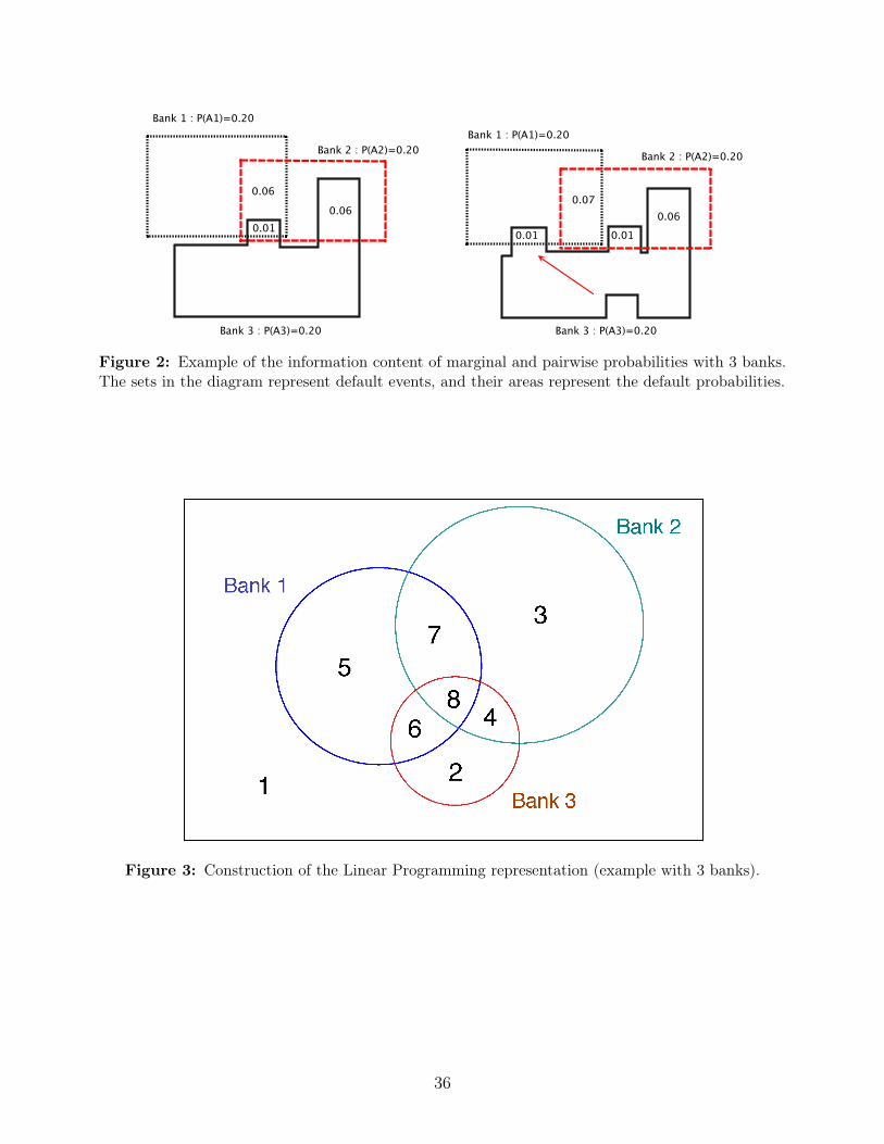
Bank 1 : P(A1)=0.20

Bank 2 : P(A2)=0.20

Bank 3 : P(A3)=0.20

0.010.06

0.06 0.07

0.010.06

Bank 1 : P(A1)=0.20Bank 2 : P(A2)=0.20

Bank 3 : P(A3)=0.20

0.01

Figure 2: Example of the information content of marginal and pairwise probabilities with 3 banks.The sets in the diagram represent default events, and their areas represent the default probabilities.

Figure 3: Construction of the Linear Programming representation (example with 3 banks).

36

Figure 4: Upper and lower bounds on systemic events under the assumption that liquidity premia ofbonds issued by financial firms increased during the crisis by at least as much as those of nonfinancialfirms. Pr is the monthly probability of at least r banks defaulting, for r = 1, 2, 3, 4. Bounds aresmoothed with a 3-day moving average.

37

Figure 5: Bounds on the monthly probability of at least 1 bank (top panel) and 4 banks (bottomthree panels) defaulting under different liquidity assumptions. The top panel shows P1 with liquiditycalibrated to nonfinancials. The bottom three panels show P4 under the three liquidity assumptions:nonnegative, at least as high as 2004, and calibrated to nonfinancials.

38

Figure 6: Bounds on P4 (probability that at least 4 banks default) under different information sets.

0.27% 0.19%

0.13%

0.39%

0.35%

0%-0.13%

0%-0.13%

0.11%-0.13%

0.06

%-0.

13%

0.17

% -

0.19

%

0.13% - 0.19%

0.11%

- 0.1

3%

0.07% - 0.13%

0.33% - 0.35%

MS Citi

JPM

Lehman

Merrill

0% - 0.13%

Figure 7: Marginal and pairwise average monthly default probabilities for part of the network inthe high systemic risk scenario (max P4) as of 08/06/2008, with the liquidity process calibrated tothat of nonfinancial firms. Nodes report the marginal default probabilities of each bank, edges reportranges for the pairwise joint default probabilities.

39

2007 20080

0.002

0.004

0.006

0.008

0.01

LehmanMerrillCity

2007 20080

1

2

3

4x 10−3

Lehman & MerrillCity & MerrillCity & Lehman

Figure 8: Marginal and pairwise default probabilities for selected banks, under the calibration ofthe liquidity process to that of nonfinancial firms, at the upper bound for the probability that at least4 banks default. A 3-day moving average is plotted.

2007 2008 2009 20100

1

2

3

4

5

6

7

8x 10−3

Prob

abilit

y th

at b

ank

is in

volv

ed in

sys

tem

ic d

efau

lt of

at l

east

4

CitiLehmanMerrillBofAOthers

Figure 9: Individual contributions to systemic risk for selected banks, under the calibration of theliquidity process to that of nonfinancial firms, at the upper bound for the probability that at least 4banks default. A 2-week moving average is plotted.

40

Figure 10: Upper and lower bounds on systemic events under the assumption that liquidity premiaof bonds issued by financial firms increased during the crisis by as much as those of nonfinancialfirms. Pr is the monthly probability of at least r banks defaulting, for r = 1, 2, 3, 4. Bounds aresmoothed with a 3-day moving average.

41

Figure 11: Bounds on the probability that at least 4 banks default (P4, shaded) against estimatesof P4 using a multivariate normal model calibrated to match the marginal default probabilities (solidlines). The different solid lines correspond to different values of ⇢, the correlation parameter of themultivariate normal distribution (assumed to be the same for all pairs). From the bottom to the top,each solid line represents the calibrated P4 for ⇢ = 0.5, 0.7, 0.9, 0.99 respectively.

42