This paper does not necessarily represent the views of the Office of the Comptroller of

the Currency. Please do not quote without permission. Comments welcome. I thank

Agostino Capponi, Mike Carhill, Darrell Duffie, Jon Gregory, Andrew Lo, Mark

Levonian and Roger Tufts for useful comments.

Dissecting the Financial Crisis of 2008:

the Role of Credit Valuation Adjustments

Akhtar Siddique1

Enterprise Risk Analysis Division

Office of the Comptroller of the Currency

Washington, DC 20219

Akhtarur.siddique@occ.treas.gov

Xian Sun

Carey Business School

Johns Hopkins University

100 International Drive

Baltimore, MD, 22043

Xian.sun@jhu.edu

1 Corresponding author.

1

Abstract

This study presents different models for computing credit valuation adjustment (CVA)

and the value at risk for CVA that permit stochastically correlated defaults across

counterparties as well as dependence between changes in exposures and default

probabilities. Using these models, it then analyzes how traditional risk measures would

have performed in measuring credit valuation adjustment (CVA) losses of financial

institutions during the crisis of 2008. A corollary to this analysis is the question of how

well would financial institutions have been capitalized for CVA risk given the risk

measures they traditionally employ. The results show that, given how the credit markets

behaved in 2008, a capital buffer based on a traditional risk measure, such as value at risk

at 99th

percentile, would have been inadequate for the mark-to-market losses incurred by

the average bank. Even "stressed VaR" likely would not have sufficed. Given common

practice and information used to compute VaR prior to 2008, capital held at a 99.9th

percentile would have been about one-half of the CVA losses.

2

Dissecting the Financial Crisis of 2008: the Role of Credit Valuation Adjustments

I. Introduction

The Financial Crisis of 2007-2009 has created significant interest in the connectedness of

financial institutions. Because of the financial innovation, players in the financial system

have established extensive business ties between them, many of which have become

prevalent in the last decade. Billio et al. (2012) present that four main financial sectors

including banks, brokers, hedge funds and insurance companies, have become highly

interrelated over the past decade. Allen et al. (2012) also show that the emergence of

financial instruments has improved the overlaps in their portfolios. Understanding how

the increased connectedness and commonality of financial institutions contributes to the

recent Financial Crisis is key to understanding of systemic risk.

While there is an increasing interest in studying the interrelation of financial

institutions and its impact on systemic risk, one area that has not received much

discussion at least from researchers’ perspective is the counterparty risk. Counterparty

risk is a byproduct of derivative products and involves not only the value of the

underlying assets, but also the survival of the participating parities of the derivative

products. AIG sold hundred billions of credit default swaps (CDS) to counterparties who

needed default protection of their investments in collateralized debt obligations (CDOs).

After the burst of the housing bubble, much of the CDOs backed by subprime loans

declined in value. Failing to post adequate amount of collateral to maintain its credit

rating and thus facing default, AIG was eventually bailed by the US government to

prevent a systemic crisis rippled through its counterparty chains.

AIG’s case is not an isolated incident and the recent credit crisis shined a bright

light on the complexities of the financial system and revealed the substantial impact of

3

counterparty risk, measured by credit valuation adjustments (CVA), on financial

institutions. For example, twelve large financial institutions reported a total of $63 billion

in CVA losses on their 2008 financial statements, albeit in the footnotes.2 These losses

needed to be recognized as a result of the requirements of FAS 157 under US GAAP or

IAS 39 under international accounting standards. Credit valuation adjustments also were

ascribed a substantial role in the losses suffered by large financial institutions by the

financial press34

.

The regulators’ rationale of requesting financial institutions recognizing CVA

losses is to provide a reasonable estimate of their exposure to counterparty default risk

(for example, the collapse of AIG increased many financial institutions’ recognition of

CVA losses because of their investment in CDS issued by AIG). Because credit valuation

adjustments are model dependent, how meaningful such estimates are, therefore, depends

heavily on how well the estimation models are defined. This study considers different

models for default as well as different models to compute credit valuation adjustments.

2 Table 1 summarizes CVA related losses reported in the footnotes to the 2008 financial statements by 12

large internationally active banks. 3 Market Watch, Jan 7, 2008, “Merrill writes off $11.5 bln, swings to $9.8 bln loss…..Merrill also made

$2.6 billion in credit-valuation adjustments related to hedges on CDOs.” 4 Structured Credit Investor, June 11, 2008, “Canadian Imperial Bank of Commerce (CIBC) has suffered

… US$4.7bn in write-downs of monoline protection to-date was on US$7.9bn of notional exposure, much

of it to ACA Financial Guaranty Corp.

The Royal Bank of Scotland Group (RBSG) disclosed a notional amount of US$12bn in credit protection

against RMBS and ABS CDOs in April 2008. RBSG has taken US$4.4bn in cumulative credit value

adjustments on all the credit protection it purchased from monolines, including protection on segments

outside of RMBS and ABS CDOs.

Credit Agricole reported US$9.9bn of notional credit protection related to ABS CDOs at 31 March 2008.

The fair value of CA's credit protection across all asset classes was US$3.4bn, after US$3.9bn in

cumulative write-downs of monoline coverage.

UBS disclosed that the notional amount of credit protection it purchased from monoline bond insurers at 31

March 2008 was US$24.6bn, of which US$11.6bn related to ABS CDOs. The fair value of its credit

protection across all asset classes was US$6.3bn, after a cumulative credit valuation adjustment of

US$2.6bn.

Societe Generale disclosed that, as of 31 March 2008, it had US$11bn in notional credit protection

purchased from monolines to hedge ABS CDOs. The fair value of its credit protection across all asset

classes was US$1.2bn, after cumulative write-downs of US$1.6bn of monoline protection and the effect of

purchased hedges.”

4

These include stochastic correlated hazard rates and also permit dependence between the

exposures and default. Using such models, this study analyzes how traditional risk

measures would have performed in measuring CVA losses for financial institutions. Note

that regulatory capital as well as internal capital at institutions before the crisis was most

commonly based on Value at Riskm a corollary to this analysis is the question is how

well financial institutions would have been capitalized for the CVA risk given the risk

measures they traditionally employ.

We obtain CDS spreads on 31 large financial institutions at tenors of 1 year, 2

years and 5 years. There are a total of 2,103 daily observations over the period January 2,

2002 through May 10, 2010. We then use six risk factors to simulate the exposures to

counterparty risk, which includes not only on the creditworthiness of the counterparties

but also on the credit worthiness of the institution. The argument is there are some

common factors impacting both the creditworthiness of the counterparties and the

investing institution. These are (1) Three month LIBOR (LIBOR3M), (2) the yield on

BAA rated bonds (BAA), (3) the spread between yields on BAA and AAA rated bonds

(BAA-AAA), (4) the return on the S&P500 index (SPX), (5) the change in the volatility

option index (VIX) and (6) Contract interest rates on commitments for fixed-rate first

mortgages (from the Freddie Mac survey) (MORTG).

We simulate 10,000 market scenarios every day. Each market scenario

corresponds to a realization of the six correlated risk factors (as multivariate unit normal

factors) which are then translated into end-of-period portfolio values. We simulate small

daily changes in each of the portfolios using uniform random variates. We update the

data daily and the market risk factors for the most recent 180 calendar days are used to

5

construct the variance-covariance matrix that is used to generate the exposures. There are

31 counterparty exposures in each of the 10,000 scenarios on each date.

From these counterparty exposures, we construct the expected exposures for the

three tenors and the CVA is then constructed for that date. Using 120 trading days of

CDS spreads for each of the 31 counterparties, 120 hypothetical CVA are calculated for

each of the 120 days. The change in the credit valuation adjustment from one period to

the next is the component in P&L arising from credit valuation adjustments. We can

compute the change in CVA (CVA), for each date. The 99th

percentile of the CVA is

its Value at Risk. This VaR is the VaR of change in CVA or CVA-VaR in shorthand.

This estimation is rolled one trading day forward at a time. Thus, the CVA-VaR is

recalculated every day. We consider different compositions of the portfolio across the

four risk factors and the distributions of exposures across the tenors. The first portfolio

we consider is an equally weighted one across the risk factors and the three tenors. The

comparison of the hypothetical CVA-VaR to the CVA suggests that the CVA-VaR would

have backtested well, except for two periods, around 2003 and again around 2009. In

both cases, the VaR would have declined very rapidly.

An important question is the adequacy of the capital buffer computed using the

value at risk measure. This can be phrased as whether a multiplier is needed on Value-at-

Risk to reduce the number of exceptions to a stated frequency. Thus, for the 99th

percentile CVA-VaR, the question is what is the minimum multiplier needed to reduce

the number of backtest exceptions to 1 in every 100 trading days. This also measures how

much additional capital beyond the 99% value at risk would have been necessary given

the realized losses.

6

As a starting point, over 1,924 trading days, the number of exceptions is 20 or

1.04%. As a first approximation, a multiplier of 1.05 would have brought the number of

exceptions to 19, i.e., less than 1%. However, given that exceptions are clustered over

time, a more relevant question is what is the multiplier needed to keep the exception rate

to 1% or less every year. Assuming 250 consecutive trading days in a year, the multiplier

is then based on the maximum number of exceptions in any consecutive 250-day period.

This required multiplier is 2.0. Therefore, if the multiplier had been 2.0 on the 99th

percentile CVA-VaR, the number of back test exceptions would have been 1%.

Therefore, if an institution had held capital for losses attributable to CVA at a

99% confidence level using a VaR approach, the capital buffer would have been only half

as large as the maximum losses in any consecutive 250 day period. This counts not only

the number of exceptions but also the magnitude of exceptions relative to the actual

losses.

The results in this paper show that, given how the credit markets behaved in 2008,

a capital buffer based on a traditional risk measure, such as value at risk at 99th

percentile,

would have been inadequate. Given the actual losses, capital buffers based on a 99%

value at risk (VaR) measure would not have been adequate. This capital would have

needed to be at least doubled to cover the actual losses.

The regulatory responses to the financial crisis of 2008 have included various

measures to strengthen the risk calculations. A regulatory response to the role played by

CVA in the financial crisis is the capitalization of CVA risk in the revised Basel III

capital rules. Incorporating stressed environments into the calculations is an important

7

element of the new capital rule. We find that stressed inputs would not have substantially

ameliorated the inadequacy of the capital measures.

We study the connectedness among financial institutions through their exposure

to counterparty risk, which gained significant visibility in the wake of the global financial

crisis. Although Billio et al. (2012) show the increasing interrelation among financial

institutions, one weakness of principle component analysis is it does not offer insights on

the factors that drive the common movement. Our contribution to literature is by

identifying a specific channel through which banks are interrelated, we quantify the value

impact of such exposure and justify the economic significance of bailing out systemically

important financial institutions.

Asymmetric unilateral CVA in risk management and pricing contexts has been

analyzed rather extensively in Brigo and Masetti (2005), Brigo and Pallanvicini (2007),

Brigo and Chourdakis (2008), and Brigo and Bakkar (2009). Unilateral CVA ignores that

changes in the credit environment can affect both the counterparties in a transaction. The

study by Brigo and Capponi (2009) is closest to our study by analyzing CVA

symmetrically in a bilateral context. These studies have analyzed CVA in a pricing and

risk management context. However, the relation between CVA and capitalization of

CVA, and the role of CVA in the financial crisis that affected banks in 2008 have not

been analyzed to our knowledge.

Our first two sections describe two models for measuring credit valuation

adjustments. Section IV describes the data. The fifth section presents the results. The

final section concludes.

II. Simple Model for Unilateral Credit Valuation Adjustment with Constant

Hazard Rates

8

Following Canabarro and Duffie (2003), we define credit valuation adjustments of an

OTC derivatives portfolio as “the market value of the credit risk due to any failure to

perform on agreements with that counterparty.” We model the “unilateral” CVA, i.e., the

impact of the counterparties’ credit quality on the institution’s valuations, but ignoring

the effect of the institution’s own credit quality on the value of its liabilities.

The unilateral CVA at time t for an institution with N counterparties is defined as

1

, ,

1

,N

j

N

j t j t t

j

CVA t CVA j t

P EE DF

(1)

where ,j tP is the jth counterparty’s probability of default at time t, ,j tEE is the expected

positive exposure to the jth counterparty at time t, and tDF is the discount factor at time t.

The discount factor does not depend on the counterparty. The probability of default and

the exposures are computed under the pricing (or risk neutral) measure. With a term

structure of exposures, we would compute the sum over the term structure as well.

We assume that the mark to market values of the OTC derivatives portfolios are

driven by a set of market risk factors,tX .

tX have a conditional multivariate normal

distribution.

t tX N μ,ΣF (2)

We simulate the distribution of the market risk factors at maturities (tenors) of 1 year, 3

years and 5 years. We then model OTC derivative portfolio values at each of the tenors

by using a set of factor sensitivities.

9

We then compute the expected exposures at 1 year, 3 year and 5 year maturities.

We then construct CVA from the expected exposures. The factor sensitivities are drawn

from a normal distribution. The correlation matrix amongst the risk factors on a date is

computed using the observations over a fixed window preceding that date.

Current exposures are modeled as negative for odd numbered counterparties and

positive for even numbered counterparties.5A granularity assumption is set to produce a

homogeneous portfolio. Factor sensitivities are randomly generated and normalized to

have a norm of 1. The value of the trades with each counterparty at each t=1, 3 or 5 are

assumed to be a linear function of the market risk factors6. Expected mark to market gain

to a counterparty is computed as the average across mktN randomly generated market risk

factor scenarios.

0

1 1

1(i)= l,i + i,k f l,k m i

mktN K

h

l kmkt

V VN

(3)

Where mktN = the number of market scenarios and

K = the number of market risk factors.

0 l,iV = the initial value of the portfolio with the ith counterparty in the lth scenario.

i,k =the factor sensitivity of the ith counterparty to the kth risk factor. \

5 These assumptions regarding current exposures are the same as same as ISDA/LIBA/TBMA (2003) and

Gibson (2005), and the model used to generate exposures is quite similar to the formulation used in annex 3

of the paper by the ISDA counterparty credit risk working group. 6 We have also carried out the simulations with convexity in the exposures as well i.e.

2

0

1 1

1(i)= l,i + i,k f l,k m i i,k f l,k m i

mktN K

h

l kmkt

V VN

. The results do

not change materially.

10

f l,k = the simulated realization on the kth risk factor in the lth scenario.

m i = -1 or +1 based on whether the counterparty is odd or even, i.e. whether the bank

has a positive exposure or negative exposure.

Expected exposure is computed as ,0hMax V i . Expected positive exposure can then

be computed as the weighted average across the three tenors.

We obtain the risk neutral probabilities of default ,j tP directly from CDS spreads.

We assume a constant recovery rate of 40% on defaulted exposures. To convert the CDS

spreads into one-year default probabilities, we used the “market approximation” with a

40% recovery assumption, i.e.,

,

,

11

11 0.40

j t t

j t

PCDS

(4)

This model of computing the credit valuation adjustment effectively assumes a

constant hazard rate that is recalibrated at each time t. Value at Risk for credit valuation

adjustment can be constructed in several different ways. For the unilateral credit

valuation adjustment model presented in section II, we use historical simulation.

III. Bilateral Credit Valuation Adjustment with Correlated Stochastic Hazard

Rates

Assuming that the hazard rates can be inferred directly from the CDS premia ignores that

default probabilities may contain predictable components. Inferring hazard rates also

ignores the fact that changes in default probabilities across institutions are likely to be

11

affected by common factors. CDS premia also contain information about a term structure

of default probabilities.

To accommodate these features, we develop a model of CVA under stochastic

hazard rates that are correlated through common factors. This approach also allows us to

consider bilateral CVA, i.e. a CVA metric that depends not only on the creditworthiness

of the counterparties but also on the credit worthiness of the institution. As a

consequence, the total CVA for an institution may change not only because changes in

the credit worthiness of its counterparties but also changes in its own credit worthiness,

i.e. in the debit valuation adjustment (DVA), sometimes referred to as Liability CVA.

We need to rely on a CDS pricing model to infer the stochastic hazard rates. We

rely on a variant of Hull and White (2000). We assume that recovery rates are constant

and defaults are independent of interest rates. We use the CDS premia to bootstrap the

survival probabilities for 1 year, 3 years and 5 years. We need to model two

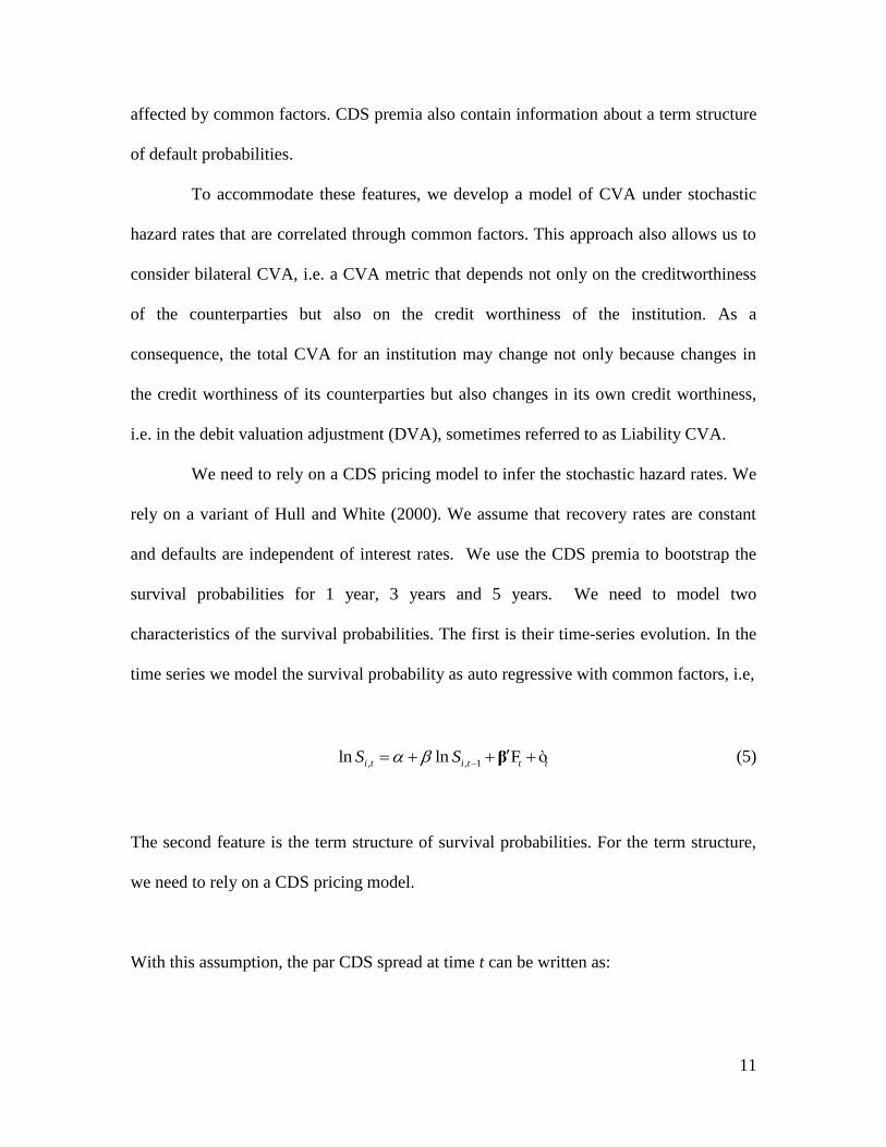
characteristics of the survival probabilities. The first is their time-series evolution. In the

time series we model the survival probability as auto regressive with common factors, i.e,

, , 1ln ln Fi t i t t tS S β ò (5)

The second feature is the term structure of survival probabilities. For the term structure,

we need to rely on a CDS pricing model.

With this assumption, the par CDS spread at time t can be written as:

12

1, ,

1

,

1

1

M

t j t j t

j

N

t k k t

t

k

R

CDS Spread

DF S S

DF S

(6)

where R is the recovery rate, tDF is the discount factor at time t,

k represents the time

increment.

We then simulate the market risk factors and rely on the parameter estimates of

the hazard rate process to construct the predicted survival probabilities. The predicted

survival probabilities then depend on the simulated market risk factors as well. The

unilateral CVA with stochastic hazard rates can be written as:

1

,

1

,N

j

N

j t t

j

t t t

CVA t CVA j t

P X E X DF

F

(7)

where , ,tt tjP X E X respectively denote the default probability of the jth counterparty

and the positive exposure with respect to the jth counterparty. The CVA is computed as a

conditional expectation using the information at time t.

Taking the debit valuation adjustment, DVA into account, the bilateral CVA, net of

DVA, may be written as:

*

1,

, ,

1,

, ,k

t

N

j j k

N

j t t t k t t t

j j

t t t

k

CVA t CVA j t CVA k t

P X E X DF P X E X DF

F F

(8)

13

For the bilateral credit valuation adjustment, we use monte carlo simulation to generate

the distribution of the underlying risk factors. We then compute the exposures and

probabilities of default jointly and compute the Value at Risk of the credit valuation

adjustment.

IV. Data

We obtain CDS spreads on 31 large financial institutions at tenors of 1 year, 2 years and

5 years. These are BBVA, BNP Paribas, Banco Santander, Bank of America, Barclays,

Charles Schwab, Citigroup, Commerzbank, Credit Agricole, Credit Lyonnais, Credit

Suisse, Deutsche Bank, Dresdner Bank, Goldman Sachs, HSBC, JP Morgan Chase,

Lehman Brothers, Lloyds, Merrill Lynch, MetLife, Mitsubishi-UFJ, Mizuho, Morgan

Stanley, National Australia Bank, RBS, Societe General, Sumitomo-Mitsui, UBS,

Unicredito, Wachovia, and Wells Fargo. The average 5 Year CDS spread for these 31

institutions is plotted in figure 1. During the crisis of 2008 and 2009, the CDS spreads

widened substantially.

It is important to note that not every bank has a quote available every day,

particularly in the earlier part of the sample period. There are a total of 2,103 daily

observations over the period January 2, 2002 through May 10, 2010. We use six risk

factors to simulate the exposures. These are (1) Three month LIBOR (LIBOR3M), (2)

the yield on BAA rated bonds (BAA), (3) the spread between yields on BAA and AAA

rated bonds (BAA-AAA), (4) the return on the S&P500 index (SPX), (5) the change in

the volatility option index (VIX) and (6) Contract interest rates on commitments for

14

fixed-rate first mortgages (from the Freddie Mac survey) (MORTG). These are explicit

factors and are plotted in figure 2. For a few dates, when the BAA or BAA-AAA is

missing, it is replaced by its lag. MORTG is in a weekly frequency which we convert to

daily data through imputation using a markov chain monte carlo.

V. Empirical Results

A. Results for Unilateral Credit Valuation Adjustment with Constant Hazard

Rates

Using the framework outlined above, we simulate 10,000 market scenarios every day.

Each market scenario corresponds to a realization of the six correlated risk factors (as

multivariate unit normal factors) which are then translated into end-of-period portfolio

values. An important consideration in constructing EPE (and other risk metrics such as

Value at Risk measures) is the frequency with which the data are updated.

We construct 5 portfolios (as weights across the risk factors)

(1) Balanced: Equally weighted

(2) Long-vol with a substantially greater weight on the VIX

(3) Short-Vol with a substantial short loading on the ViX

(4) Long-credit with a substantial long loading on BAA-AAA (junk spread)

(5) Short Credit with substantial short loading on BAA-AAA.

We construct the EPE using both unstressed parameters and stressed parameters.

In each case we use histories using 180 days of data as well as 750 days to compute the

parameters. The stress period is assumed to end with 2009/06/30. We simulate small

daily changes in each of the portfolios using uniform random variates. The weights are

15

then multiplied by the simulated risk factors for that day. 100,000 multivariate normal

distributed random variates using a Sobol sequence are used.

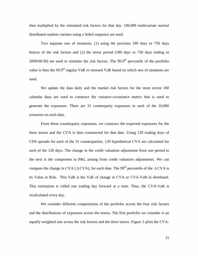
Two separate sets of moments, (1) using the previous 180 days or 750 days

history of the risk factors and (2) the stress period (180 days or 750 days ending in

2009/06/30) are used to simulate the risk factors. The 99.9th

percentile of the portfolio

value is then the 99.9th

regular VaR or stressed VaR based on which sets of moments are

used.

We update the data daily and the market risk factors for the most recent 180

calendar days are used to construct the variance-covariance matrix that is used to

generate the exposures. There are 31 counterparty exposures in each of the 10,000

scenarios on each date.

From these counterparty exposures, we construct the expected exposures for the

three tenors and the CVA is then constructed for that date. Using 120 trading days of

CDS spreads for each of the 31 counterparties, 120 hypothetical CVA are calculated for

each of the 120 days. The change in the credit valuation adjustment from one period to

the next is the component in P&L arising from credit valuation adjustments. We can

compute the change in CVA (CVA), for each date. The 99th

percentile of the CVA is

its Value at Risk. This VaR is the VaR of change in CVA or CVA-VaR in shorthand.

This estimation is rolled one trading day forward at a time. Thus, the CVA-VaR is

recalculated every day.

We consider different compositions of the portfolio across the four risk factors

and the distributions of exposures across the tenors. The first portfolio we consider is an

equally weighted one across the risk factors and the three tenors. Figure 3 plots the CVA-

16

VaR and the average CDS premia. From the graph, it appears that the VaR would have

tracked changes in the levels of the CDS premia reasonably well with the exception of

2009.

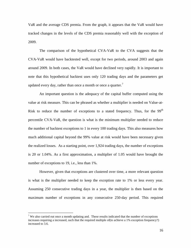
The comparison of the hypothetical CVA-VaR to the CVA suggests that the

CVA-VaR would have backtested well, except for two periods, around 2003 and again

around 2009. In both cases, the VaR would have declined very rapidly. It is important to

note that this hypothetical backtest uses only 120 trading days and the parameters get

updated every day, rather than once a month or once a quarter.7

An important question is the adequacy of the capital buffer computed using the

value at risk measure. This can be phrased as whether a multiplier is needed on Value-at-

Risk to reduce the number of exceptions to a stated frequency. Thus, for the 99th

percentile CVA-VaR, the question is what is the minimum multiplier needed to reduce

the number of backtest exceptions to 1 in every 100 trading days. This also measures how

much additional capital beyond the 99% value at risk would have been necessary given

the realized losses. As a starting point, over 1,924 trading days, the number of exceptions

is 20 or 1.04%. As a first approximation, a multiplier of 1.05 would have brought the

number of exceptions to 19, i.e., less than 1%.

However, given that exceptions are clustered over time, a more relevant question

is what is the multiplier needed to keep the exception rate to 1% or less every year.

Assuming 250 consecutive trading days in a year, the multiplier is then based on the

maximum number of exceptions in any consecutive 250-day period. This required

7 We also carried out once a month updating and. These results indicated that the number of exceptions

increases requiring a increased, such that the required multiple of(to achieve a 1% exception frequency?)

increased to 3.6.

17

multiplier is 2.0. Therefore, if the multiplier had been 2.0 on the 99th

percentile CVA-

VaR, the number of back test exceptions would have been 1%.

Therefore, if an institution had held capital for losses attributable to CVA at a

99% confidence level using a VaR approach, the capital buffer would have been only half

as large as the maximum losses in any consecutive 250 day period. This counts not only

the number of exceptions but also the magnitude of exceptions relative to the actual

losses. We then consider some other portfolio compositions. Table 2 summarizes the

various permutations across tenor and risk factors. In all the cases considered, the 99th

percentile CVA-Value at Risk would have been inadequate.

B. Results for Bilateral Credit Valuation Adjustment with Correlated

Stochastic Hazard Rates

For the bilateral credit valuation adjustment, we need to estimate (5). We use generalized

method of moments to estimate the parameters of the following:

1 1 1 1

0, 0, 1, 2, 1,

3 3 3 3

0, 0, 1, 2, 3,

1 1

, , 1

3 3

, , 1

5 5

,

5 5 5 5

0, 0, 11 , 2 5, , ,

ln ln BAA_AAA Vix

ln ln BAA_AAA Vix for banks

ln ln BAA_AAA Vix

Y Y

i t i t

Y Y

i t i t

Y Y

i t i t

Y Y Y Y

i i i t i t t

Y Y Y Y

i i i t i t t

Y Y Y Y

i i i t i t t

S S

S S i

S S

ò

ò

ò

1,31 (9)

The parameters, 1 1 1 1

0, 0, 1, 2,, , , ,Y Y Y Y

i i i i 1, ,j 3 3

0, 0,,Y Y

i i 3 3 5 5 5 5

1, 2, 0, 0, 1, 2,, , , , , ,Y Y Y Y Y Y

i i i i i i describe

the hazard rate process for generalized method of moments. We normalize the systematic

factors to have a mean of zero.

Table 3 presents the coefficients from (9) for each of the 31 institutions. It is

interesting to note that there is great variation across the banks in how important the

common factors are in determining the changes in survival probabilities. The survival

probabilities are also very persistent as shown by the very significant 0,i coefficients for

18

almost all of the institutions for all three tenors. BAA_AAA generally is more significant

at for the 3 and 5 year survival probabilities whereas Vix is more significant for the 1

year survival probability.

We simulate small daily changes in each of the portfolios using uniform random

variates. The weights are then multiplied by the simulated risk factors for that day.

100,000 multivariate normal distributed random variables using a Sobol sequence are

used. In the simulation of the risk factors two separate sets of moments, (1) using the

previous 180 days or 750 days history of the risk factors and (2) the stress period (180

days or 750 days ending in 2009/06/30) are used.

The simulated risk factors are then multiplied by the weights to obtain the

exposure. The same simulated risk factors are used in (9) to generate the predicted

survival probabilities. The data is updated daily. The market risk factor data for the most

recent 180 calendar days are used to construct the variance-covariance matrix that is used

to generate the exposures.

Thus in each scenario, there are 31 <default probability, exposure> pairs. We

assume that the institution #17 has exposures to the other 30 institutions. We then

construct the credit valuation adjustment for each scenario by aggregating across the 30

counterparties and subtracting institution #17's own valuation adjustment. We then

aggregate across the scenarios taking the probabilities into account. These calculations

result in the bilateral credit valuation adjustment for institution #17 each day. The change

in the credit valuation adjustment from one period to the next is the component in P&L

arising from credit valuation adjustments.

19

We then use historical simulation to compute the 99th

percentile of CVA as the

Value at Risk. That VaR is the VaR of change in CVA or CVA-VaR in shorthand. We

use look-back periods of 180 days, 360 days and 750 days. Figures 5 shows respectively

the CVA and CVA-VaR using computed using a default model using correlated

stochastic hazard rates and bilateral CVA.

We again find that CVA-VaR computed using bilateral CVA and correlated

stochatic hazard rates would not have been adequate to capitalize for the CVA. The 99th

percentile CVA-VaR would need to be multiplied by 2.4 to be adequate. This is true for

both regular calibration as well as stressed calibration of the simulation engine.

Conclusions

This paper relies on a highly stylized portfolio. Nevertheless, it suggests that the

development of an appropriately risk sensitive CVA-VaR is fraught with difficulties.

Backtest exceptions suggest (but can not prove) that the model is not consistent with

reality.

The results show that, given how the credit markets behaved in 2008, a capital

buffer based on a traditional risk measure, such as value at risk at a 99th

percentile,

would, on average, have been inadequate. A capital buffer computed using a 99% VaR

measure would have been only one-half of the amount required to ensure that losses

would not exceed the 99% threshold.

In future work, we intend to relax some of the simplifying assumptions used here.

These would address the assumption of a constant hazard rate in deriving the

probabilities of default, as well as the assumptions that the risk factors are normally

20

distributed and that the exposures are linear in the risk factors. Both non-normality and

non-linearity are likely to produce more exceptions, and hence the multiplier on value at

risk would likely need to be higher, indicating that the extent of the shortfall in the capital

buffer based on VaR would likely have been even higher.

21

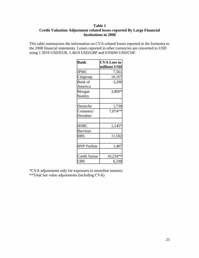
Table 1

Credit Valuation Adjustment related losses reported By Large Financial

Institutions in 2008

This table summarizes the information on CVA-related losses reported in the footnotes to

the 2008 financial statements. Losses reported in other currencies are converted to USD

using 1.3919 USD/EUR, 1.4619 USD/GBP and 0.93694 USD/CHF.

Bank CVA Loss in

millions USD

JPMC 7,561

Citigroup 10,107

Bank of

America

3,200

Morgan

Stanley

3,800*

Deutsche 1,730

Commerz/

Dresdner

7,074**

HSBC 1,145*

Barclays

RBS 11,502

BNP Paribas 1,407

Credit Suisse 10,234**

UBS 6,100

*CVA adjustments only for exposures to monoline insurers.

**Total fair value adjustments (including CVA)

22

Table 2

This table presents the results of different portfolio compositions on the requisite

multiplier to the 99th

percentile CVA-Value at Risk to ensure that exceptions are no more

frequent that 1%. The relative weights across the tenors and risk factors in the

composition of the portfolio are expressed as fractions.

Tenors 1 Year = 1/3 2 Years = 1/3 3 Years = 1/3

Risk Factors VIX =1/4 S&P500 =1/4 BAA-AAA =1/4 BAA=1/4

Multiplier =2.00

Tenors 1 Year = 1/4 2 Years = 1/4 3 Years =1/ 2

Risk Factors VIX =1/5 S&P500 =1/5 BAA-AAA =2/5 BAA=1/5

Multiplier =2.00

Tenors 1 Year = 1/3 2 Years = 1/3 3 Years = 1/3

Risk Factors VIX =1/3 S&P500 =1/6 BAA-AAA =1/3 BAA=1/6

Multiplier =1.60

Tenors 1 Year = 1/3 2 Years = 1/3 3 Years = 1/3

Risk Factors VIX =2/5 S&P500 =1/5 BAA-AAA =1/5 BAA=1/5

Multiplier =2.00

0

Table 3

Models for the Evolution of Survival Probabilities

This table presents the parameters from the estimation of the survival probability evolution model: 1 1 1 1

0, 0, 1, 2, 1,

3 3 3 3

0, 0, 1, 2, 3,

1 1

, , 1

3 3

, , 1

5 5

,

5 5 5 5

0, 0, 11 , 2 5, , ,

ln ln BAA_AAA Vix

ln ln BAA_AAA Vix for banks

ln ln BAA_AAA Vix

Y Y

i t i t

Y Y

i t i t

Y Y

i t i t

Y Y Y Y

i i i t i t t

Y Y Y Y

i i i t i t t

Y Y Y Y

i i i t i t t

S S

S S i

S S

ò

ò

ò

1,31

The parameters are estimated in a fully identified GMM system.

Bank Wachovia

Credit

Suisse

Mitsuibishi

UFJ

Natitional

Australia UBS Deutsche HSBC

BNP

Paribas RBS Barclays 1

0

Y -0.00510* -0.00019* -0.00134*** -0.00028* -0.00028 -0.00019 -0.00016 -0.00013 -0.00016 -0.00018

1

0

Y 0.83072*** 0.99234*** 0.92676*** 0.98761*** 0.99068*** 0.99049*** 0.99151*** 0.99060*** 0.99305*** 0.99260***

1

1

Y 0.00034 0.00004 0.00010 0.00003 0.00009 0.00004 0.00003 0.00003 0.00016** 0.00005

1

2

Y 0.18728* 0.00697 0.04468*** 0.01047 0.01218 0.00682 0.00637 0.00472 0.00675 0.00717

3

0

Y -0.01565* -0.00037 -0.00133*** -0.00052** -0.00084* -0.00057* -0.00037* -0.00026 -0.00074* -0.00061*

3

0

Y 0.78649*** 0.99326*** 0.96309*** 0.98936*** 0.98883*** 0.98811*** 0.99164*** 0.99198*** 0.98924*** 0.99023***

3

1

Y 0.00114** 0.00005 0.00017** 0.00003 0.00009 0.00008** 0.00002 0.00002 0.00010 0.00012**

3

2

Y 0.61995 0.01424 0.04532*** 0.01947* 0.03689* 0.02252 0.01460 0.00959 0.03114 0.02614

5

0

Y -0.01232 -0.00018 -0.00081** -0.00029 -0.00061* 0.00025 -0.00023 0.00002 -0.00018 -0.00032

5

0

Y 0.87915*** 0.99582*** 0.98230*** 0.99357*** 0.99321*** 1.00170*** 0.99467*** 0.99921*** 0.99720*** 0.99515***

1

5

1

Y 0.00114** 0.00005 0.00017** 0.00003 0.00009 0.00008** 0.00002 0.00002 0.00010 0.00012**

5

2

Y 0.47248 0.00808 0.02714* 0.01433 0.02864* -0.00764 0.01079 0.00134 0.00925 0.01444

Coefficients significant at 10%, 5% and 1% are identified with *, ** and ***, respectively.

2

Bank Unicredito Dresdner JPMC

Wells

Fargo BAC Citi

Goldman

Sachs

Morgan

Stanley MetLife Schwab 1

0

Y -0.00031* -0.00011 -0.00016 -0.00031** -0.00036* -0.00070* -0.00163* -0.00312 -0.00463*** -0.01446***

1

0

Y 0.98784*** 0.99285*** 0.99140*** 0.98689*** 0.98974*** 0.98772*** 0.96021*** 0.94570*** 0.94588*** 0.41996***

1

1

Y 0.00002 0.00003 0.00002 0.00004 0.00003 0.00016 0.00000 0.00064* 0.00068 -0.00019

1

2

Y 0.01214* 0.00326 0.00489 0.01098* 0.01442 0.02978 0.06120* 0.12956 0.20145*** 0.48752***

3

0

Y -0.00057* -0.00024 -0.00032 -0.00048 -0.00054 -0.00118 -0.00315*** -0.00845 -0.00771*** -0.02548***

3

0

Y 0.98977*** 0.99383*** 0.99277*** 0.99116*** 0.99289*** 0.99126*** 0.96484*** 0.93733*** 0.95821*** 0.44435***

3

1

Y 0.00004 0.00003 0.00000 -0.00001 -0.00003 0.00006 0.00003 0.00047 -0.00051 0.00061

3

2

Y 0.02310* 0.00801 0.01031 0.01724 0.02124 0.05061 0.12294*** 0.35421 0.32271*** 0.84437***

5

0

Y -0.00018 -0.00016 -0.00001 -0.00043 -0.00010 -0.00096 -0.00083 -0.00440 -0.00350 -0.02530***

5

0

Y 0.99659*** 0.99572*** 0.99635*** 0.99345*** 0.99735*** 0.99356*** 0.98979*** 0.96936*** 0.98370*** 0.62028***

5

1

Y 0.00004 0.00003 0.00000 -0.00001 -0.00003 0.00006 0.00003 0.00047 -0.00051 0.00061

5

2

Y 0.00977 0.00705 0.00301 0.01984 0.01072 0.05472 0.03814 0.22167 0.16986 0.81332***

Coefficients significant at 10%, 5% and 1% are identified with *, ** and ***, respectively.

3

Bank Merrill Lynch

Credit Lyonnais

Credit Agricole SocGen Lehman

Banco Santander Commerzbank Lloyds

Sumitomo Mitsui Mizuho BBVA

1

0

Y -0.00084*** -0.00272*** -0.00081*** -0.00018 -0.00212*** -0.00014 -0.00009 -0.00024 -0.00163*** -0.00188*** -0.00038*

1

0

Y 0.98023*** 0.84485*** 0.95354*** 0.99047*** 0.90285*** 0.99228*** 0.99243*** 0.99030*** 0.89831*** 0.90595*** 0.98054***

1

1

Y 0.00005 0.00002 0.00008* 0.00004 -0.00021 0.00001 0.00001 0.00005 0.00013 0.00019** 0.00001

1

2

Y 0.03005*** 0.09596*** 0.02955** 0.00669 0.05266*** 0.00453 0.00146 0.00942 0.05192*** 0.05811*** 0.01392*

3

0

Y -0.00100 -0.00279** -0.00106* -0.00038* -0.00296*** -0.00034 -0.00021 -0.00061* -0.00168*** -0.00178*** -0.00056**

3

0

Y 0.98803*** 0.92131*** 0.97046*** 0.99126*** 0.93605*** 0.99300*** 0.99411*** 0.99026*** 0.94622*** 0.95536*** 0.98712***

3

1

Y 0.00021 0.00000 0.00007 0.00004 0.00025 0.00004 0.00005 0.00000 0.00017* 0.00013 0.00004

3

2

Y 0.03658 0.09970*** 0.03925** 0.01516 0.08256*** 0.01289 0.00617 0.02501 0.05220*** 0.05346*** 0.02133*

5

0

Y -0.00067 -0.00162*** -0.00066*** 0.00010 -0.00282* -0.00015 -0.00007 -0.00041 -0.00081** -0.00071* -0.00022

5

0

Y 0.99306*** 0.96978*** 0.98780*** 1.00050*** 0.95468*** 0.99638*** 0.99674*** 0.99572*** 0.97890*** 0.98417*** 0.99592***

5

1

Y 0.00021 0.00000 0.00007 0.00004 0.00025 0.00004 0.00005 0.00000 0.00017* 0.00013 0.00004

5

2

Y 0.02924 0.05618** 0.02666*** -0.00241 0.06952** 0.00767 0.00305 0.01966 0.02692* 0.02505* 0.01042

Coefficients significant at 10%, 5% and 1% are identified with *, ** and ***, respectively.

16

References

Allen, F., Babus, A., Carletti, E., 2012. Asset commonality, debt maturity and systemic risk. Journal of

Financial Economics 104, 51-534.

Billio, M., Getmansky, M., Lo, A. W., Pelizzon, L. 2012. Econometric measures of connectedness and

systemic risk in the finance and insurance sector. Journal of Financial Economics 104, 535-559.

D. Brigo and K. Chourdakis. Counterparty Risk for Credit Default Swaps: Impact of spread volatility

and default correlation, forthcoming in International Journal of Theoretical and Applied Finance, 2008.

D. Brigo, I. Bakkar. Accurate counterparty risk valuation for energy-commodities swaps. Energy Risk.

March 2009 issue.

D. Brigo and M. Masetti. Risk Neutral Pricing of Counterparty Risk. In: Pykhtin, M. (Editor),

Counterparty Credit Risk Modeling: Risk Management, Pricing and Regulation. Risk Books, 2005,

London.

D. Brigo and A. Pallavicini. Counterparty Risk under Correlation between Default and Interest Rates. In:

Miller, J., Edelman, D., and Appleby, J. (Editors). Numerical Methods for Finance, Chapman Hall,

2007.

D. Brigo and A. Capponi Bilateral counterparty risk valuation

with stochastic dynamical models and application to Credit Default Swaps, manuscript, 2009.

Counterparty Risk Treatment of OTC Derivatives and Securities

Financing Transactions, June 2003

ANNEX 3 – CALCULATION OF ECONOMIC CAPITAL BASED

ON EPE, http://www.isda.org/c_and_a/pdf/counterpartyriskannex.pdf

E. Canabarro and D. Duffie, Chapter 9: Measuring and Marking Counterparty Risk, ALM of Financial

Institutions, Institutional Investor Books, 2004.

M. Gibson. Measuring Counterparty Credit Exposure to a

Margined Counterparty. U.S Federal Reserve working paper, 2005, 50.

16

Figure 1: Time series Plot of Average CDS Premia

0

50

100

150

200

250

300

20020328

20020624

20020918

20021212

20030312

20030606

20030902

20031125

20040224

20040519

20040816

20041109

20050204

20050503

20050728

20051021

20060119

20060417

20060712

20061005

20070103

20070330

20070626

20070920

20071214

20080313

20080609

20080903

20081126

20090225

20090521

20090817

20091110

20100208

20100505

Date

Av

era

ge

CD

S

Average_CDS

Figure 2: Time series Plot of Risk Factors

0

10

20

30

40

50

60

70

80

90

20020102

20020402

20020702

20021002

20030102

20030402

20030702

20031002

20040102

20040402

20040702

20041002

20050102

20050402

20050702

20051002

20060102

20060402

20060702

20061002

20070102

20070402

20070702

20071002

20080102

20080402

20080702

20081002

20090102

20090402

20090702

20091002

20100102

20100402

Date

VIX

Clo

se

-15

-10

-5

0

5

10

15

BA

A-A

AA

or

BA

A o

r S

&P

50

0

Re

turn

VIX Close BAA_AAA S&P500 BAA

17

Figure 3: Time series Plot of Average CDS Premia & CVA-VaR

0

50

100

150

200

250

20020102

20020402

20020702

20021002

20030102

20030402

20030702

20031002

20040102

20040402

20040702

20041002

20050102

20050402

20050702

20051002

20060102

20060402

20060702

20061002

20070102

20070402

20070702

20071002

20080102

20080402

20080702

20081002

20090102

20090402

20090702

20091002

20100102

20100402

Date

Av

era

ge

CD

S

-0.00500.0050.010.0150.020.0250.030.0350.040.045

CV

A -

Va

R

Average_CDS CVA_VaR

Figure 4: Time series Plot of CVA_VaR and Change in CVA

0.00

0.00

0.01

0.01

0.02

0.02

0.03

0.03

0.04

20020918

20021218

20030318

20030618

20030918

20031218

20040318

20040618

20040918

20041218

20050318

20050618

20050918

20051218

20060318

20060618

20060918

20061218

20070318

20070618

20070918

20071218

20080318

20080618

20080918

20081218

20090318

20090618

20090918

20091218

20100318

Date

CV

A V

aR

an

d C

ha

ng

e in

CV

A

CVA_VaR CVA

18

-500

-400

-300

-200

-100

0

100

200

300

400

500

20

04

12

22

20

05

02

25

20

05

04

29

20

05

07

01

20

05

09

02

20

05

11

04

20

06

01

10

20

06

03

15

20

06

05

17

20

06

07

20

20

06

09

21

20

06

11

22

20

07

01

30

20

07

04

03

20

07

06

06

20

07

08

08

20

07

10

10

20

07

12

12

20

08

02

15

20

08

04

21

20

08

06

23

20

08

08

25

20

08

10

27

20

08

12

30

20

09

03

05

20

09

05

07

20

09

07

10

20

09

09

11

20

09

11

12

20

10

01

19

20

10

03

23

Figure 5: Change in Bilateral CVA and VaR of Change in Bilateral CVA Using 750 preceding days to compute VaR

Bilateral CVA VaR of Bilateral CVA