Credit card interchange fees ∗

Jean-Charles Rochet† Julian Wright‡

January 23, 2009

Abstract

We build a model of credit card pricing that explicitly takes into account credit func-

tionality. We show that a monopoly card network always selects an interchange fee that

exceeds the level that maximizes consumer surplus. If regulators only care about consumer

surplus, a conservative regulatory approach is to cap interchange fees based on retailers’

net avoided costs from not having to provide credit themselves. In the model, this always

raises consumer surplus compared to the unregulated outcome, sometimes to the point of

maximizing consumer surplus.0

1 Introduction

Even through payment cards are gradually becoming the most popular and most efficient means

of payments in many countries, there is a growing suspicion surrounding the pricing of credit

cards. Retailers complain that the fees they have to pay to accept credit card transactions are out

of proportion with the costs incurred by banks. Some competition authorities and central banks

have suggested banks provide consumers with exaggerated incentives to use their credit cards, to

the detriment of other means of payments like cash and debit cards which they believe to be more

efficient. The usual suspects are the interchange fees, the transfer fees paid by the bank of the

retailer to the banks of the cardholders, which are often considerably higher than those for debit

∗We benefited from the helpful comments of conference participants at the AEA January 2009 meeting in San

Francisco (especially our discussant, Charlie Kahn) and two Conferences on Payments Economics at the Central

Bank of Norway (November 2008) and the Central Bank of Canada (November 2008).†Toulouse School of Economics. Email: rochet@cict.fr‡Department of Economics, National University of Singapore: E-mail: jwright@nus.edu.sg.

1

cards.1 In the past several years, there have been more than 50 lawsuits concerning interchange

fees filed by merchants and merchant associations against card networks in the United States,

while in about 20 countries public authorities have take regulatory actions related to interchange

fees and investigations are proceeding in many more (Bradford and Hayashi, 2008).

Given the obvious importance of understanding how interchange fees should be set, this article

analyzes credit card interchange fee determination to see whether there are grounds for regulatory

intervention, and if so, in what form. The point of departure from the existing literature is to

model credit cards explicitly. An existing literature models price determination in payment cards

networks, initiated by Schmalensee (2002), Rochet and Tirole (2002) and Wright (2003).2 The

models in this literature have essentially focused on the choice between payment cards (which

could just as well be debit cards) and cash (or checks). We contribute to this literature by

extending the models to allow a separate role for the credit functionality of credit cards, thereby

allowing us to discuss credit card interchange fees specifically.3

In our model, credit cards can be used for two types of transactions — “ordinary purchases”

for regular convenience usage for which cash (or a debit card) are assumed to provide identical

benefits, and for “credit purchases” where credit is necessary for purchases to be realized. Credit

purchases include a range of different types of purchases (such as unplanned purchases, impulse

purchases and large purchases) for which the consumer does not have the cash or funds imme-

diately available to complete the purchase or for purchases for which the deferment of

payment facilitates the transaction. For ordinary purchases, we assume credit cards are

inefficient given we assume there are additional costs of transacting with credit cards. As a result,

card networks which maximize profit by maximizing the number of card transactions have an in-

centive to encourage over-usage of credit cards by convenience users (even when these consumers

do not need the credit facility) provided merchants still accept such credit card transactions. A

card network does this by setting interchange fees high enough to induce issuers to offer rewards

and cash back bonuses (equivalent to negative fees). On the other hand, the alternative to using

credit cards for credit purchases is the direct provision of credit by merchants or “store credit”,

1Unregulated credit card interchange fees are typically between 1% to 2% of transaction value, whereas debit

card interchange fees are typically between 0% and 1%. See, for instance, Charts 2 and 3 in Weiner and Wright

(2005).2See also Baxter (1983) for a much earlier treatment, and Rochet (2003) for a survey of the literature.3Among the few papers to model explicitly the credit functionality are Chakravorty and To (2007) and more

recently Bolt and Chakravorty (2008), although these papers do not focus on the determinant of interchange fees

for credit cards, nor the regulation of these fees.

2

which is assumed to be relatively inefficient. Since consumers do not internalize retailers’ cost

savings from avoiding direct provision of credit and since merchants cannot distinguish the type

of consumer they face, there is also a case for setting a relatively high interchange fee so that

consumers that wish to rely on credit are induced to use credit cards when it is efficient for

them to do so. For this reason, to maximize consumer surplus (including the surplus of cash

customers) may require setting an interchange fee which induces excessive usage of credit

cards for ordinary purchases.

Taking into account both types of transactions, a monopoly card network always sets its

interchange fee too high in our setting. Thus, if regulators only care about (short-run) consumer

surplus, our theory can provide a rationalization for placing a cap on interchange fees.4 The

theory suggests one of two possible caps will maximize consumer surplus. Depending on the

relative costs and benefits of the different instruments, the cap should either be based on the

issuers’ costs (to avoid excessive usage of cards for ordinary purchases) or on merchants’

net avoided costs from not having to provide credit directly (so that consumers use their cards

efficiently for credit purchases). Since evaluating which of the two options gives higher consumer

surplus is informationally very demanding, a conservative regulatory approach would be to cap

interchange fees using the maximum of these two levels, which is likely to be the latter option.

In our model, this always raises consumer surplus compared to the unregulated outcome, and will

sometimes result in the best outcome for consumers. In contrast, using issuer costs to regulate

interchange fees is realistically only likely to give a lower bound of possible interchange fees

that maximize consumer surplus.

2 The Model

There is a continuum of consumers (of total mass normalized to one) with quasi-linear preferences.

They spend their income on a composite good taken as a numeraire and on retail goods costing

γ to produce. There are two payment technologies: cash (which could also capture cheques and

debit cards5) and credit cards. Credit cards are assumed to be more costly but allow consumers

4In focusing on consumer surplus, we ignore the need for issuers to recover fixed costs and the effect this has

on entry incentives (and therefore, on long-run consumers surplus). We also ignore the need to get consumers to

internalize the effect of their decisions on the profit of issuers so as to maximize total welfare. As Rochet and

Tirole (2008) show, taking these effects into account justifies higher interchange fees.5Since the focus of this paper is on the provision of consumer credit, we do not introduce any differences

between pure payment technologies. Such differences are discussed at length in the literature mentioned in the

3

to purchase on credit. They are held by a fraction x of consumers, where x is initially taken

as given.6 Consumers purchase one unit of the retail good (what we call “ordinary purchases”)

providing them with utility u0 with u0 > γ. In addition, with probability θ, they also receive

utility u1 from consuming another unit of the retail good (what we call “credit purchases”). We

assume that merchants cannot bundle the two transactions and also cannot distinguish between

“ordinary” and “credit” purchases. We assume that each consumer has always enough cash to

pay for his ordinary purchases, but must rely on credit for credit purchases.

Each retailer can directly provide credit to the consumer (“store credit”), but this entails a

cost cB for the consumer (buyer) and cost cS to the retailer (seller). The cost cS is the same

for all credit purchases from a given seller, but cB is transaction specific, and is observed by

the consumer only when he is in the store. cB is drawn from a continuous distribution with the

cumulative distribution function H. We assume the distribution has full support over some range

(cB , cB) where cB is sufficiently negative, such that cardholders will sometimes choose to

use store credit, and cB is positive but not too high (in comparison with u1 − γ), such that

consumers will always prefer to make the credit purchase (even if they have to pay with

store credit) than not buy at all.7 Initially, we assume cB only arises with respect to

credit purchases, and represents the net cost of using store credit rather than credit

cards for credit purchases, which is why we allow the possibility of negative draws

of cB . In section 4 we will analyze what happens when cB is instead interpreted as

a transaction cost that arises equally for ordinary purchases and credit purchases.

Given the costs of store credit, accepting credit cards is a potential means for merchants

to reduce their transaction costs of accepting credit purchases and to increase the quality of

service to buyers. The cost of a credit transaction is cA for the bank of the merchant (which

is called the acquirer of the transaction) and cI for the bank of the cardholder (the issuer of

the card). The total cost of a credit card transaction is thus c = cA + cI . Bank fees for credit

card transactions are denoted f for consumers and m for merchants. When f < 0 (cash back

bonuses) consumers prefer to also use their credit cards for ordinary purchases, which given our

assumptions is socially wasteful.8 For each credit card transaction, an interchange fee a is paid

introduction, e.g. Schmalensee (2002), Rochet and Tirole (2002) and Wright (2003).6In section 4 we extend the model to allow consumers to decide whether to join the card network or not.7Without this assumption, credit card acceptance would not just add value by reducing the

transaction costs of arranging credit; it would also lead to an increase in the volume of credit

purchases, which would provide an additional factor affecting efficient interchange fees.8We assume consumers and retailers face no costs of using cash (which can be thought of as a normalization).

For ordinary purchases, any costs or benefits to consumers and retailers of using cash are assumed to be the

4

by the bank of the merchant (the acquirer) to the bank of the consumer (the issuer).

For simplicity, we assume that acquiring merchants is perfectly competitive for banks, which

implies that the merchant fee m is equal to the sum of the acquiring cost cI and the interchange

fee a:

m = cI + a. (1)

By contrast, we assume that issuers are imperfectly competitive: the cardholder fee f is equal

to the net issuer cost cI − a plus a profit margin π, assumed for simplicity to be constant. We

thus have:

f(a) = cI − a + π. (2)

These assumptions are not made to necessarily capture any intrinsic asymmetry

between the nature of competition in issuing and acquiring, the existence of which

is an empirical matter. Rather, the main reason for making these particular as-

sumptions on bank competition is that they provide a simple setting in which card

networks seek to maximize profit by maximizing the number of card transactions.

The level of the interchange fee a has an impact on retailer cost and thus on the retail price9

p(a), which results from competition between retailers. To model competition between retailers,

we use the standard Hotelling model: consumers are uniformly distributed on an interval of

unit length, with one retailer (i = 1, 2) located at each extremity of the interval. Transport

cost for consumers is t per unit of distance. We consider the case where credit card service are

provided by a single network (monopoly). Its objective is to maximize total profits of its member

banks, which is proportional to total volume of credit card transactions. As noted above, this

simplification is due to our assumption that banks’ profit margins are constant (0 for acquirers,

π for issuers).

The timing of our model is as follows:

• The card network sets the interchange fee a so as to maximize banks’ total profit.

• Banks set their fees: f(a) = cI − a + π for cardholders and m(a) = cA + a for retailers.

• Retailers independently choose their card acceptance policies: Li = 1 if retailer i accepts

credit cards, 0 otherwise.

same as those obtained from using credit cards (which can be thought of as an approximation).9We assume that retailers cannot, or do not want to, charge different retail prices for cash and card payments

(i.e. no surcharging).

5

• After observing (L1, L2), retailers independently set retail prices p1, p2.

• Consumers observe retail prices and card acceptance policies and select one retailer to

patronize.

• Once the consumer is in the store, he buys a first unit of the retail good (“ordinary pur-

chase”), and pays it by cash or a credit card (if he has one).

• Finally, nature decides whether he has an opportunity for a credit purchase (this occurs

with probability θ) and in this case, the cost cB of using store credit for the buyer is drawn

according to the c.d.f. H, with full support on [cB , cB ]. Cardholders then select their mode

of payment.

In the framework above we assumed that consumers sometimes will obtain a negative draw

of cB (i.e. cB < 0). This was one way to ensure store credit is not dominated by credit cards.

Despite this, we also assumed store credit is never used for ordinary purchases. We did this

by assuming that for ordinary purchases consumers can only choose between cash and credit

cards, consistent with the net cost of using store credit always being positive for

ordinary transactions. This helps to simplify the analysis. Subsequently, we will show

our results continue to hold even when consumers may sometimes prefer store credit

for ordinary purchases. Another reason why store credit may not be dominated by credit

cards is that some consumers will not want to hold credit cards unless the costs of doing so are

sufficiently subsidized (or they receive sufficient rewards for doing so). We, thus, also analyze an

alternative specification in which we endogenize the choice by consumers of whether to hold a

credit card in the first place but then assume the cost to consumers of using store credit cB is

always positive. These two extensions are analyzed in Section 4.

3 Analysis and policy implications

We first analyze the model to derive optimal interchange fees. This involves determining when

retailers will accept credit cards so as to determine what interchange fees a card network will

set. We then compare this to the interchange fees that maximize consumer surplus and derive

some policy implications.

6

3.1 When Do Retailers Accept Credit Cards?

This section derives the equilibrium behavior of retailers as a function of the fundamental policy

variable in our model, namely the interchange fee a. We first construct a retailer’s profit function.

We will use the notation Lc = 1 if f < 0, Lc = 0 if f ≥ 0 to distinguish whether credit

cards are used for ordinary purchases or not. A fraction 1 − xLi of the time, consumers cannot

use credit cards. For ordinary purchases, such consumers must therefore use cash. For credit

purchases, which happen with probability θ, these consumers will always use store credit. A

fraction xLi of the time, consumers can also use credit cards. For ordinary purchases, these

cardholders will use cash if f ≥ 0 (i.e. if Lc = 0) and credit cards if f < 0 (i.e. if Lc = 1).

For credit purchases, which happen with probability θ, these cardholders will use store credit if

cB < f but otherwise will use credit cards. Collecting together a retailer’s margins associated

with each of these different possibilities, retailer i’s expected margin per-customer is therefore

equal to

Mi = (1 − xLi) (pi − γ + θ (pi − γ − cS))

+xLi (pi − γ − Lcm + θ (H (f) (pi − γ − cS) + (1 − H (f)) (pi − γ − m)))

or after simplifying

Mi = (1 + θ) (pi − γ) − θcS − xΓ (a) Li,

where

Γ(a) = Lcm + θ (m − cS) (1 − H (f))

is the retailer’s expected net cost per-cardholder from accepting cards as a function of the inter-

change fee.

Corresponding to each of the different types of possible transactions, retailer i offers an

expected surplus (ignoring transportation costs) of

Ui = (1 − xLi) (u0 + θu1 − (1 + θ) pi − θE (cB))

+xLi

(

u0 + θu1 − (1 + θ) pi − Lcf − θ

(

∫ f

cB

cBdH (cB) +

∫ cB

f

fdH (cB)

))

or after simplifying

Ui = u0 + θu1 − (1 + θ) pi − θE (cB) + xS (a) Li,

where

S (a) = −Lcf + θ

∫ cB

f

(cB − f) dH (cB)

7

is the expected net consumer surplus per-cardholder from credit card usage as a function of the

interchange fee. Determining retailer i’s market share by finding the indifferent consumer in the

normal way, we find10

si =1

2+

(1 + θ)(pj − pi)

2t+ xS (a)

Li − Lj

2t. (3)

Retailer i’s profit function can then be written πi = Misi. Let us denote by φ(a) the difference

between S(a) and Γ(a), which we call total user surplus:

φ(a) = S(a) − Γ(a) = θ

∫ cB

cI+πI−a

(cB + cS − c − πI)dH(cB) − (c + πI)Lc. (4)

The first term represents total expected surplus of the two users (consumers and retailers) from

using credit cards for consumers’ credit purchases. The second term is a deadweight loss asso-

ciated with the use of credit cards for ordinary purchases. We are now ready to derive

the equilibrium choices of retailers. We first derive equilibrium resulting from price competition

between retailers for given card acceptance decisions L1, L2.

Proposition 1 For any couple L1, L2 of card acceptance decisions, price competition between

retailers leads to retail prices such that

(1 + θ)p∗i = t + γ(1 + θ) + θcS + xΓ(a)Li +x

3φ (a) (Li − Lj) . (5)

Retailers’ profits are π∗

i = 2t (s∗i )2, where retailer i’s equilibrium market share si is

s∗i =1

2+

xφ (a) (Li − Lj)

6t. (6)

Proof of Proposition 1: See the Appendix.

So as to maximize profit, each retailer chooses to accept cards if it increases its market share,

which will be the case whenever φ (a) ≥ 0. An immediate consequence of Proposition 1 is:

Proposition 2 Retailers accept credit cards at equilibrium if and only if expected consumer

surplus from card transactions exceeds expected retailer cost. That is, L∗

1 = L∗

2 = 1 if and only if

φ(a) ≥ 0, i.e. S (a) ≥ Γ(a).

10We assume that t is large enough so that each retailer always has a positive market share at equilibrium

(0 < si < 1 for all i). We also assume that u0 + θu1 is large enough so that all the market is served (Ui > tsi for

all i).

8

3.2 Analysis of Retailer Prices and Consumer Surplus

This section considers the impact of the interchange fee a on consumer surplus. Obviously this

question only matters in the region where S(a) ≥ Γ(a), i.e. when credit cards are accepted.

Proposition 1 allows us to compute retail prices and consumer surplus as a function of a.

Considering the case where L1 = L2 = 1 and thus p1(a) = p2(a) = p(a), formula (5) gives

(1 + θ)p(a) = t + γ(1 + θ) + θcS + xΓ(a). (7)

Since Γ(a) (the expected net retailer cost from card transactions) increases in a we obtain an

immediate corollary of Proposition 1.

Corollary 1 The equilibrium retail price is an increasing function of the interchange fee a.

The expected surplus of cash consumers (those not holding credit cards) is

Ucash(a) = u0 + θu1 −t

4− (1 + θ) p (a) − θE (cB)

and of consumers holding credit cards is

Ucredit(a) = u0 + θu1 −t

4− (1 + θ)p(a) − Lcf − θ

(

∫ f

cB

cBdH (cB) +

∫ cB

f

fdH (cB)

)

.

If we aggregate the surplus of all consumers (cash consumers and cardholders) and take into

account equilibrium prices from (7), we obtain

CS(a) = xUcredit(a) + (1 − x) Ucash(a)

= u0 + θu1 − γ (1 + θ) −5t

4− θ (E (cB) + cS) + xφ(a).

Thus, aggregate consumer surplus is equal, up to an additive and a positive multiplicative con-

stants, to total user surplus φ(a).

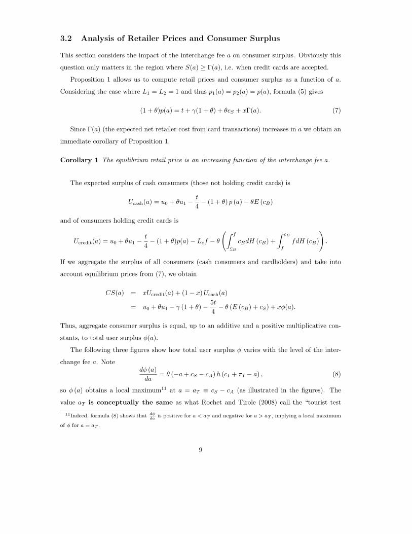
The following three figures show how total user surplus φ varies with the level of the inter-

change fee a. Notedφ (a)

da= θ (−a + cS − cA) h (cI + πI − a) , (8)

so φ (a) obtains a local maximum11 at a = aT ≡ cS − cA (as illustrated in the figures). The

value aT is conceptually the same as what Rochet and Tirole (2008) call the “tourist test

11Indeed, formula (8) shows that dφda

is positive for a < aT and negative for a > aT , implying a local maximum

of φ for a = aT .

9

threshold”, i.e. the maximum level of the interchange fee such that the merchant fee m = cA +a

is less than the cost cS of the relevant alternative technology (i.e. which in a credit card setting

is store credit) for the merchant. This threshold is also conceptually equivalent to the

interchange fee recommended by Baxter (1983) in the context of a perfectly competitive banking

sector, and to Farrell’s (2006) “Merchant Indifference Criterion”. Note, however, aT is not

necessarily a global maximum for total user surplus φ. This is because φ has a downward jump

at a = a∗ ≡ cI + πI . This jump is due to the fact that when a > a∗, cardholder fee f becomes

negative, and cardholders find it convenient to use their credit card for ordinary purchases. In

formula (6) this is captured by the fact that Lc = 1 if and only if a > a∗, implying a

downward jump of magnitude c+πI for total user surplus φ. This jump complicates the analysis

of consumer surplus maximisation, and introduces three regimes.

In regime 1, aT = cS − cA is less than a∗ ≡ cI + πI , and therefore total user surplus is

maximized for a = aT . This corresponds to the situation where credit card transactions are more

costly to provide than retailer provided store credit:

cS − cA ≤ cI + πI ⇔ cS ≤ c + πI .

In regime 1, regulation to maximize consumer surplus would require making sure credit cards

were priced to be more expensive for consumers than using cash (or debit cards).

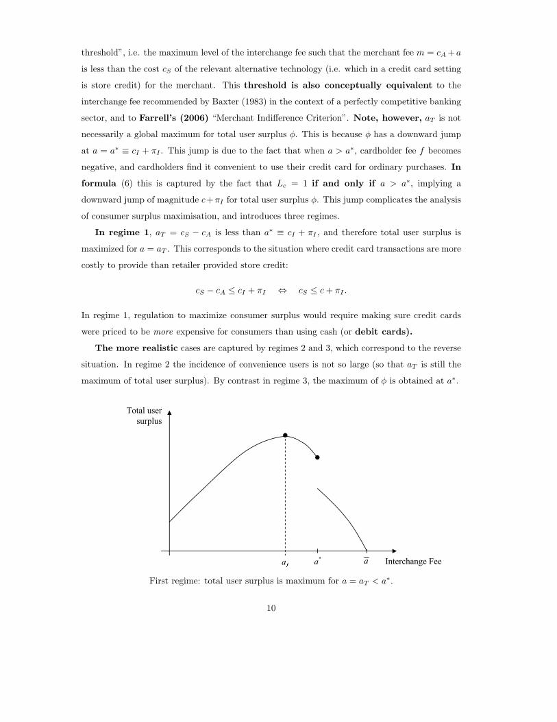
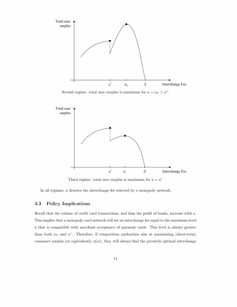
The more realistic cases are captured by regimes 2 and 3, which correspond to the reverse

situation. In regime 2 the incidence of convenience users is not so large (so that aT is still the

maximum of total user surplus). By contrast in regime 3, the maximum of φ is obtained at a∗.

First regime: total user surplus is maximum for a = aT < a∗.

10

Second regime: total user surplus is maximum for a = aT > a∗.

Third regime: total user surplus is maximum for a = a∗

In all regimes, a denotes the interchange fee selected by a monopoly network.

3.3 Policy Implications

Recall that the volume of credit card transactions, and thus the profit of banks, increase with a.

This implies that a monopoly card network will set an interchange fee equal to the maximum level

a that is compatible with merchant acceptance of payment cards. This level is always greater

than both aT and a∗. Therefore, if competition authorities aim at maximizing (short-term)

consumer surplus (or equivalently φ(a)), they will always find the privately optimal interchange

11

fee excessive.12 A regulatory cap on interchange fees can therefore be justified but the appropriate

level of the cap is not always the same: it is aT in regime 2 and a∗ in regime 3. Which of these

regimes is relevant depends on the magnitude of the difference between cS , the retailer’s cost

of providing store credit and c + πI , the total user cost of credit transactions. We denote this

difference by δ ≡ cS − c − πI . These results are recapitulated in the next proposition:

Proposition 3 If regulatory authorities aim at maximizing (short-term) consumer surplus, pri-

vately optimal interchange fees are too high. A regulatory cap on interchange fees can therefore

raise (short-term) consumer surplus, but two cases must be considered, depending on the value

of δ = cS − c − πI :

a) If δ < 0 (regime 1) or if c + πI ≤ θ∫ 0

−δ(cB + δ) dH (cB) (regime 2), the regulatory cap

should be aT = cS − cA.

b) Otherwise (regime 3), the regulatory cap should be a∗ = cI + πI .

Proof of Proposition 3: See the Appendix.

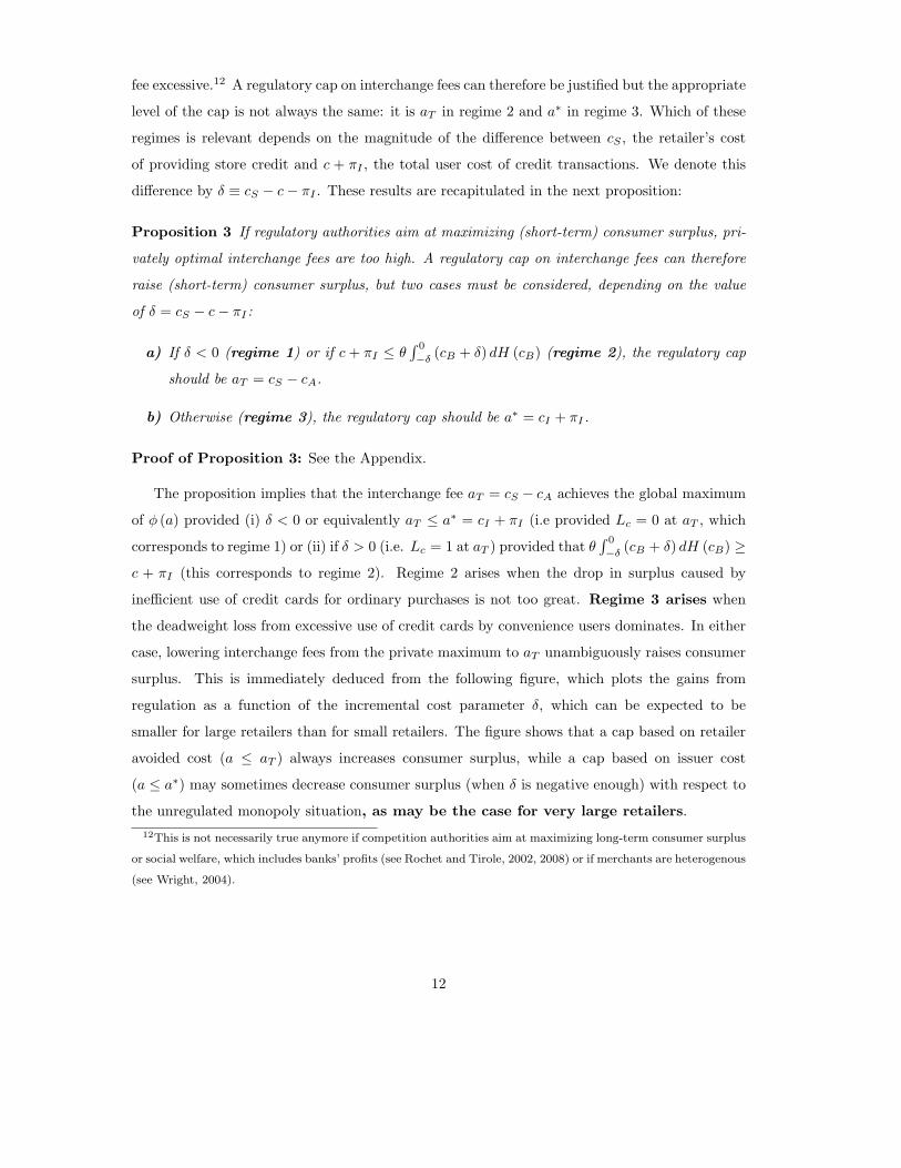
The proposition implies that the interchange fee aT = cS − cA achieves the global maximum

of φ (a) provided (i) δ < 0 or equivalently aT ≤ a∗ = cI + πI (i.e provided Lc = 0 at aT , which

corresponds to regime 1) or (ii) if δ > 0 (i.e. Lc = 1 at aT ) provided that θ∫ 0

−δ(cB + δ) dH (cB) ≥

c + πI (this corresponds to regime 2). Regime 2 arises when the drop in surplus caused by

inefficient use of credit cards for ordinary purchases is not too great. Regime 3 arises when

the deadweight loss from excessive use of credit cards by convenience users dominates. In either

case, lowering interchange fees from the private maximum to aT unambiguously raises consumer

surplus. This is immediately deduced from the following figure, which plots the gains from

regulation as a function of the incremental cost parameter δ, which can be expected to be

smaller for large retailers than for small retailers. The figure shows that a cap based on retailer

avoided cost (a ≤ aT ) always increases consumer surplus, while a cap based on issuer cost

(a ≤ a∗) may sometimes decrease consumer surplus (when δ is negative enough) with respect to

the unregulated monopoly situation, as may be the case for very large retailers.

12This is not necessarily true anymore if competition authorities aim at maximizing long-term consumer surplus

or social welfare, which includes banks’ profits (see Rochet and Tirole, 2002, 2008) or if merchants are heterogenous

(see Wright, 2004).

12

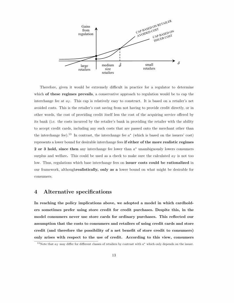
Therefore, given it would be extremely difficult in practice for a regulator to determine

which of these regimes prevails, a conservative approach to regulation would be to cap the

interchange fee at aT . This cap is relatively easy to construct. It is based on a retailer’s net

avoided costs. This is the retailer’s cost saving from not having to provide credit directly, or in

other words, the cost of providing credit itself less the cost of the acquiring service offered by

its bank (i.e. the costs incurred by the retailer’s bank in providing the retailer with the ability

to accept credit cards, including any such costs that are passed onto the merchant other than

the interchange fee).13 In contrast, the interchange fee a∗ (which is based on the issuers’ cost)

represents a lower bound for desirable interchange fees if either of the more realistic regimes

2 or 3 hold, since then any interchange fee lower than a∗ unambiguously lowers consumers

surplus and welfare. This could be used as a check to make sure the calculated aT is not too

low. Thus, regulations which base interchange fees on issuer costs could be rationalized in

our framework, althoughrealistically, only as a lower bound on what might be desirable for

consumers.

4 Alternative specifications

In reaching the policy implications above, we adopted a model in which cardhold-

ers sometimes prefer using store credit for credit purchases. Despite this, in the

model consumers never use store cards for ordinary purchases. This reflected our

assumption that the costs to consumers and retailers of using credit cards and store

credit (and therefore the possibility of a net benefit of store credit to consumers)

only arises with respect to the use of credit. According to this view, consumers

13Note that aT may differ for different classes of retailers by contrast with a∗ which only depends on the issuer.

13

never have an incentive to use store credit for ordinary purchases given credit is

not needed for these purchases. An alternative view is that the costs of store credit

measure the costs of using these instruments for transactions in general, regardless

of whether they are ordinary purchases or credit purchases. Consistent with this

view, in this section, we consider two different setting in which we assume the costs

of using each type of payment are the same across ordinary and credit purchases.

In the first setting the cost to consumers of using store credit is allowed to take

negative values. The idea is that store credit may sometimes provide benefits to

consumers even for ordinary purchases, such as possibly allowing cardholders to

preserve their funds for some other contingencies. Thus, consumers will choose be-

tween cash, store credit, and credit cards (if they hold credit cards) when making

ordinary purchases. This change in assumptions turns out only to strengthen our

main results. Second, we consider the case in which the cost of using store credit is always

positive (cB ≥ 0) so that consumers would never want to use store credit for ordinary purchases

(cash would always be preferred). Instead, we endogenize the choice by consumers of whether

to hold a credit card in the first place. We show this framework still leads to similar policy

implications to our benchmark case.

4.1 Allowing store credit for ordinary purchases

We follow the same steps as in section 3. The main impact of the additional types of possible

payment transactions is to make the definitions of the underlying terms Mi, Γ(a), S (a) and φ (a)

more complicated, while leaving the structure of the analysis largely unaffected. As we will see,

allowing consumers to choose store credit when making ordinary purchases only strengthens the

policy implications of section 3. Essentially, it increases the number of situations in which it

is desirable to have consumers internalize the cost to merchants of providing store credit, and

thereby makes it more likely that the interchange fee aT = cS − cA maximizes consumer surplus.

We start by considering the retailer’s margins and demand arising from each type of transac-

tion. A fraction 1−xLi of the time, consumers cannot use credit cards. For ordinary purchases,

these consumers will use store credit if cB ≤ 0, which happens with probability H (0); otherwise,

with probability 1 − H (0) they will prefer to use cash. For credit purchases, which happen

with probability θ, these consumers will always use store credit. A fraction xLi of the time,

consumers can also use credit cards. For ordinary purchases, these cardholders will use store

credit if cB < Lcf , and otherwise either credit cards (if Lc = 1) or cash (if Lc = 0). For credit

14

purchases, these cardholders will use store credit if cB < f and otherwise credit cards. Collect-

ing together a retailer’s margins associated with each of these different possibilities, retailer i’s

expected margin per-customer is therefore equal to

Mi = (1 − xLi) [(H (0) + θ) (pi − γ − cS) + (1 − H (0)) (pi − γ)]

+xLi

[

H (Lcf) (pi − γ − cS) + (1 − H (Lcf)) (pi − γ − Lcm)

+θ (H (f)) (pi − γ − cS) + (1 − H (f)) (pi − γ − m)]

or after simplifying

Mi = (1 + θ) (pi − γ) − (H (0) + θ) cS − xΓ (a) Li,

where

Γ(a) = (H (Lcf) − H (0)) cS + (1 − H (Lcf))Lcm + θ (1 − H (f)) (m − cS) .

Similarly, we can rewrite consumers’ expected utility and retailer i’s market share taking

into account the additional types of payment transactions that are possible. Retailer i offers an

expected surplus (ignoring transportation costs) of

Ui = (1− xLi)

(

u0 + θu1 − (1 + θ) pi −

∫

0

cB

cBdH (cB)− θE (cB)

)

+xLi

(

u0 + θu1 − (1 + θ) pi −

∫ Lcf

cB

cBdH (cB)−

∫ cB

Lcf

LcfdH (cB)− θ

(

∫ f

cB

cBdH (cB) +

∫ cB

f

fdH (cB)

))

or after simplifying

Ui = u0 + θu1 − (1 + θ) pi −

∫ 0

cB

cBdH (cB) − θE (cB) + xS (a) Li,

where

S (a) =

∫ 0

Lcf

(cB − Lcf) dH (cB) −

∫ cB

0

LcfdH (cB) + θ

∫ cB

f

(cB − f) dH (cB) .

Total user surplus can then be written

φ(a) = S(a) − Γ(a)

=

∫ 0

Lc(cI+πI−a)

(cB + cS − (c + πI) Lc) dH (cB)

+θ

∫ cB

cI+πI−a

(cB + cS − c − πI) dH (cB) −

∫ cB

0

(c + πI) LcdH (cB) .

The last two terms in φ(a) are similar to before. The first term is new, reflecting that there may

be cost savings from using credit cards for ordinary purchases if this avoids the use of more costly

15

store credit. Together, the first two terms represent total expected cost savings of the two users

(consumers and retailers) from using credit cards for consumers’ purchases (as opposed to using

store credit). The last term is the deadweight loss associated with convenience usage of credit

cards for ordinary purchases, although this now arises for fewer transactions since store credit is

now used for some ordinary transactions.

Aside from these new surplus definitions, the analysis of retailers’ decisions remains un-

changed. That is, retailer i’s market share and profit expressions remain the same, as do propo-

sitions 1 and 2. Retailer i’s equilibrium price is now given by

(1 + θ) p∗i = t + γ (1 + θ) + (H (0) + θ) cS + xΓ(a)Li +x

3φ (a) (Li − Lj) ,

where the right-hand-side includes the additional term H (0) cS arising from the use of store

credit for some ordinary purchases by cash customers.14 Consumer surplus is similarly adjusted

for this additional term, and so now equals

CS (a) = u0 + θu1 − γ (1 + θ) −5t

4−

∫ 0

cB

(cB + cS) dH (cB) − θ (E (cB) + cS) + xφ(a).

Thus, aggregate consumer surplus is still equal, up to an additive and a positive multiplicative

constants, to total user surplus φ(a).

As before φ (a) has a jump (down) at a = a∗. However, the total user surplus function is

now more likely to be maximized for a higher interchange fee. The derivative φ′ (a) is the same

as before except it is multiplied by (Lc + θ) /θ which exceeds one for a > a∗. This also implies

aT which maximizes φ (a) for a > a∗ is identical to before. That is, as before aT = cS − cA.

Proposition 3 now becomes

Proposition 4 If regulatory authorities aim at maximizing (short-term) consumer surplus, pri-

vately optimal interchange fees are too high. A regulatory cap on interchange fees can therefore

raise (short-term) consumer surplus, but two cases must be considered:

a) If δ < 0 (regime 1) or if (c + πI) (1 − H(0)) ≤ (1 + θ)∫ 0

−δ(cB + δ) dH(cB) (regime 2),

the regulatory cap should be aT = cS − cA.

b) Otherwise (regime 3), the regulatory cap should be a∗ = cI + πI .

14It is no longer the case that Γ(a) is necessarily increasing in a since Γ′(a) =

(Lc + θ) (h (f) (m − cS) + (1 − H (f))) so that for m much below cS , higher interchange fees could actu-

ally lower prices. However, for m not too much below cS (i.e. a not too much below cS − cA), then prices will

still be increasing in interchange fees.

16

The proposition implies that the interchange fee aT = cS − cA achieves the global maximum

of φ (a) provided (i) δ < 0, or equivalently aT ≤ a∗ = cI + πI (i.e provided Lc = 0 at aT ) or (ii)

if δ > 0 (i.e. Lc = 1 at aT ) provided

(1 + θ)

∫ 0

−δ

(cB + δ) dH (cB) ≥ (c + πI) (1 − H(0)) . (9)

Notice the trade-off here. The left-hand-side of (9) measures the cost saving from using credit

cards rather than store credit when credit cards have a negative fee as opposed to a zero fee. The

right-hand-side of (9) measures the additional costs to users from the use of credit cards rather

than cash for ordinary purchases when credit cards have a negative fee (and so are used whenever

cB > 0). Compared to before, the condition for case (ii) to apply is more easily satisfied since

the left-hand-side integral is the same as before except it is multiplied by 1 + θ instead of θ and

the right-hand-side integral is the same as before except it is multiplied by 1−H (0) instead of 1.

In other words, allowing for consumers to choose store credit when making ordinary purchases

only strengthens the previous policy implications.

4.2 Endogenizing card membership decisions

In this section, we consider an extension of the existing model in which consumers make prior

membership decisions, on whether to hold a credit card or not. Prior membership decisions

are potentially important since if interchange fee are set too low (for instance, at zero), then

consumers can be expected to face higher fees (for instance, the full cost of issuing cards) at

which point many consumers may choose to no longer hold credit cards. In order to simplify the

resulting model, we assume that consumers always view using store credit as costly (cB = 0).

With this assumption there is no issue about whether consumers can use store credit for ordinary

purchases; even if they could use store credit for these purchases, as was the case in section 4.1,

they would always prefer to use cash for this purpose. This assumption on cB will also imply

that, whenever f < 0, cardholders will always want to use cards if they are accepted. In this

case, cardholders will never use store credit. However, as we will see, setting an interchange fee

such that f < 0 may still be optimal for consumers (as opposed to setting an interchange fee

such that f = 0) since it induces more people to hold a credit card, thereby reducing the use of

expensive store credit for credit purchases by consumers who otherwise would not hold a credit

card.

The model is the same as before except that (i) there is an additional choice for consumers

as to whether to hold a card or not and (ii) we set cB = 0. Specifically, at the same time as

17

retailers choose their card acceptance policies (i.e. stage 3), consumers receive a random draw v

of the benefit of holding a credit card and decide whether to hold the card or not. v is drawn

according to the distribution function Ψ over the support (−∞, v] for some v > 0. Let x (a) be

the measure of consumers who join given an interchange fee a. Some consumers draw v < 0, so

they would prefer not to hold a credit card other things equal (e.g. if they didn’t expect to use

it). This could also capture that there are significant per-customer costs to issuers associated

with managing a cardholder which are passed through to cardholders. For other consumers,

cards may offer more than just the ability to make transactions at retailers, in which case v > 0

is possible.

We follow the same steps as in section 3. The assumption cB ≥ 0 is consistent with the

analysis in section 3 which assumes consumers never use store credit for ordinary purchases.

Therefore, the analysis of retailers’ decisions (which treat x as given), and the various surplus

expressions are identical to before. Note, however, that when f < 0, then 1 − H (f) = 1 since

all cardholders will use credit cards rather than store credit, which is just a special case of the

more general analysis detailed in section 3. This implies

φ (a) = θ

∫ cB

(1−Lc)f

(cB + cS − c − πI)dH(cB) − (c + πI)Lc,

which is now independent of a if a > a∗ (so that Lc = 1):

a > a∗⇒ φ(a) ≡ θ[E(cB) + cS ] − (1 + θ)(c + πI).

In order to keep the analysis interesting, we assume

θ (E (cB) + cS) > (1 + θ) (c + πI) , (10)

so that the surplus created from credit cards (the cost saving) is higher than their additional

cost to users when they are always used (i.e. when f < 0). Without making the assumption

in (10), retailers would reject cards if and only if a > a∗. Taking this into account, the card

network would set the interchange fee at a∗ and there would be no rationale for any regulation.

With (10), the card network will want to set a > a∗, after which the interchange fee is neutral

in terms of usage decisions. Retailers will always accept cards no matter how high the fees and

cardholders will always use them. From the point of view of users (in aggregate), interchange

fees beyond a∗ just represent pure transfer fees. It will therefore be optimal for the card scheme

to set interchange fees to the point where all consumers hold cards. Not surprisingly, like before,

this will lead interchange fees to be set too high.

18

Using the expressions for Ucredit(a) and Ucash(a) from section 3 but taking into account that

cB = 0, the expected additional utility to a consumer of holding a card is

Ucredit(a) − Ucash(a) = θ

∫ cB

(1−Lc)f

(cB − f) dH (cB) − Lcf

so consumers will hold cards if

v > Lcf − θ

∫ cB

(1−Lc)f

(cB − f) dH (cB)

implying x (a) = 1−Ψ(

Lcf − θ∫ cB

(1−Lc)f(cB − f) dH (cB)

)

which is increasing in a. Taking into

account the additional utility from holding a card, total consumer surplus is equal to (up to an

additive and a multiplicative constants)

∫ v

Lcf−θ∫ cB(1−Lc)f

(cB−f)dH(cB)

(v + φ (a)) dΨ(v) .

When a > a∗, this simplifies to∫ v

(1+θ)f−θE(cB)

(v + θ (E(cB) + cS) − (1 + θ) (c + πI))) dΨ(v) .

As before, total surplus has a jump (down) at a = a∗. However, the total surplus function

behaves slightly differently for a > a∗. It is maximum when

(1 + θ)f − θE(cB) = (1 + θ)(c + πI) − θ[E(cB) + cS ].

After simplifying, we obtain the optimal value of f :

f = c + πI −θ

1 + θcS .

Since f is equal to cI +πI −a, we obtain that the interchange fee aT which maximizes total user

surplus for a > a∗ is now

aT =θ

1 + θcS − cA. (11)

This is lower than aT = cS − cA in the benchmark model. Here the purpose of the optimal

interchange fee is to induce consumers to hold cards even when they otherwise would not want

to, so that they internalize retailers’ surplus from being able to accept their credit cards rather

than rely on store credit for credit purchases. Note the retailers’ surplus cS − cA only arises

a fraction θ/ (1 + θ) of the time, whereas a fraction 1 − θ/ (1 + θ) of the time, the retailer is

actually worse off by cA due to the excessive usage of cards. Following this interpretation, aT

can also be written:

aT =θ

1 + θ(cS − cA) −

(

1 −θ

1 + θ

)

cA.

19

As in Proposition 3, which of aT or a∗ maximizes consumer surplus depends on the magnitude

of the incremental cost of store cards over credit cards, which is now measured by

δ = θcS − (1 + θ)(c + πI).

Proposition 5 If regulatory authorities aim at maximizing (short-term) consumer surplus, pri-

vately optimal interchange fees are too high. A regulatory cap on interchange fees can therefore

raise (short-term) consumer surplus, but two cases must be considered:

a) If δ < 0 (regime 1) or if

∫ v

−θE(cB)

(c + πI) dΨ(v) ≤

∫

−θE(cB)

−δ−θE(cB)

(

v + δ + θE (cB))

dΨ(v) (12)

(regime 2), the regulatory cap should be aT = θ1+θ

cS − cA.

b) Otherwise (regime 3), the regulatory cap should be a∗ = cI + πI .

The proposition implies that the interchange fee aT = θ1+θ

cS − cA achieves the global maxi-

mum of φ (a) provided (i) δ < 0, or equivalently aT ≤ a∗ = cI + πI (i.e provided Lc = 0 at aT )

or (ii) if aT > a∗ (i.e. Lc = 1 at aT ) provided (12) holds. Given it may be hard to measure θ

with any confidence or to evaluate whether (12) holds or not, a conservative regulatory approach

could again be to use aT = cS − cA as the regulatory cap since according to the model this (i)

increases consumer surplus relative to the privately set interchange fee; (ii) possibly maximizes

consumer surplus; and (iii) yet is never too low from the point of view of maximizing (short-term)

consumer surplus. Thus, in this alternative framework, policy implications remain remarkably

similar to our benchmark case in section 3.

5 Conclusions

Much of the existing literature on interchange fees treats payment cards as though they were

debit cards. This paper provides a new theory of interchange fees that is specifically applicable

to credit card networks. The model we provide captures a trade-off that can arise between the

excessive usage of credit cards for ordinary purchases and the importance of getting cardholders

who do need credit to internalize retailers’ avoided costs arising from their credit card usage. In

terms of this trade-off, we find that an unregulated card network always sets the interchange fee

too high. Consumer surplus can be increased by imposing a cap on interchange fees which equals

20

the retailers’ net avoided costs from not having to provide credit themselves. Further lowering

interchange fees from this level towards issuing costs may either increase or decrease consumer

surplus, although initially consumer surplus always falls in our framework.

The possibility that the regulator’s preferred interchange fee predicted by our

theory may still be moderately high reflects the potentially high merchant benefits

of accepting cards in these circumstances, which cardholders may not otherwise

internalize. Put differently, if the interchange fee is set too low (say at zero) so that

consumers were sometimes not willing to hold or use cards for such transactions,

then competing merchants will instead tend to rely more on store credit (or other

forms of credit) so as to attract business. Quite plausibly, the additional costs to

society of making greater use of these more expensive forms of credit will outweigh

any benefit from encouraging debit rather than credit card transactions for ordinary

purchases. Some excessive use of credit cards may be unavoidable given merchants

cannot easily observe if credit is needed or not by their customers. This seems no

different from the fact merchants that offer interest-free installment plans to their

customers, will sometimes (perhaps often) end up offering these plans to consumers

who actually do not need them.

One important direction for future research is to extend our model to allow retail-

ers to offer different prices (through the use of discounts, interest-free periods and

rewards) when consumers make use of store credit. In not allowing this possibility,

we had in mind such price differentials being exogenous for each retailer, deter-

mined perhaps through an association of retailers or being absent altogether due

to the inability of retailers to set differential prices based on a consumer’s choice of

payment technology. If retailers could discriminate based on the use of store credit

they may be able to induce consumers to use credit cards and store credit efficiently.

However, any individual retailer would still not be able to (nor have the incentive

to) use its differential pricing to get consumers to make the right decision about

whether to hold a credit card in the first place. As such, our results from section

4, in which card membership is endogenized, are likely to carry over to the case

retailers can price discriminate in this way.

Another possible direction for future research is to extend our model to allow for

competing payment networks. By adapting the arguments of Guthrie and Wright

(2007) one should be able to show similar results to those shown here still hold

21

when there is competition between multiple card payment networks. The idea is

that competing networks will seek to choose an interchange fee somewhere between

the one maximizing total user surplus and that chosen by a monopoly network,

depending on the extent to which consumers choose to hold multiple cards, and so

these may still be too high.

We conclude by noting some other implications of our theory, which may be able to explain

real-world observations that have previously defied theoretical explanation. If credit is more

likely to be needed by customers for large purchases, then the optimal interchange fee should

be ad valorem in our setting (thereby better targeting the transfer to cardholders for the types

of transactions where credit is needed). Thus, the model potentially provides a justification for

the widespread use of ad valorem credit card interchange fees. It also explains why merchants

may want to reject credit cards for small transactions (where people are more likely to be able to

purchase anyway using cash). Most importantly, it explains why interchange fees are typically

lower for debit cards than for credit cards. Finally, the theory suggests large retailers that are

able to gain a competitive advantage over smaller rivals from being able to offer their own store-

credit to customers, may have an interest in opposing the widespread use of general purpose

credit cards.

22

Appendix

Proof of Proposition 1:

From the text we have

πi = ((1 + θ) (pi − γ) − θcS − xΓ (a) Li)

(

1

2+

(1 + θ)(pj − pi)

2t+ xS (a)

Li − Lj

2t

)

Differentiating we get

2t

1 + θ

∂πi

∂pi

= t + (1 + θ)(pj − pi) + xS(a)(Li − Lj) − (1 + θ)(pi − γ) + θcS + xLiΓ(a).

At a Nash equilibrium, we have for i, j = 1, 2:

(1 + θ)(2pi − pj) = t + γ(1 + θ) + θcS + x (S(a)(Li − Lj) + LiΓ(a)) .

Solving for pi, we obtain formula (5):

(1 + θ)pi = t + γ(1 + θ) + θcS + xΓ(a)Li +x

3φ (a) (Li − Lj) . (13)

Substituting (13) into (3) and using (4) implies formula (6).

Proof of Proposition 3:

It results immediately from the comparison of φ(aT ) and φ(a∗). Recall the expression of φ(a):

φ(a) = θ

∫

∞

a∗−a

(cB + cS − c − πI)dH(cB) − (c + πI)1Ia>a∗ ,

and note that δ = cS − cA − cI − πI = aT − a∗. Thus

φ(aT ) = θ

∫

∞

−δ

(cB + δ)dH(cB) − (c + πI)1Iδ>0,

while

φ(a∗) = θ

∫

∞

0

(cB + δ)dH(cB).

Thus

φ(aT ) − φ(a∗) = θ

∫ 0

−δ

(cB + δ)dH(cB) − (c + πI)1Iδ>0.

When δ < 0 we have

φ(aT ) − φ(a∗) = −θ

∫

−δ

0

(cB + δ)dH(cB) > 0

(since cB + δ ≤ 0 when cB belongs to [0,−δ]). Thus φ is maximum for a = aT .

When δ > 0 we have

φ(aT ) − φ(a∗) = θ

∫ 0

−δ

(cB + δ)dH(cB) − (c + πI).

This establishes Proposition 3.

23

References

Baxter, W.P. (1983) “Bank Interchange of Transactional Paper: Legal Perspectives,” Journal

of Law and Economics, 26: 541-88.

Bolt, W. and S. Chakravorty (2008) “Consumer Choice and Merchant Acceptance of

Payment Media,” mimeo.

Bradford, T. and F. Hayashi (2008) “Developments in Interchange Fees in the United

States and Abroad,” Payments System Research Briefing, Federal Reserve Bank of Kansas

City. April.

Chakravorty, S. and T. To (2007) “A Theory of Credit Cards,” International Journal of

Industrial Organization, 25: 583-95.

Farrell, J. (2006) “Efficiency and Competition between Payment Instruments,” Review of

Network Economics, 5: 26-44.

Guthrie, G. and J. Wright (2007) “Competing Payment Schemes,” Journal of Industrial

Economics, 55: 37-67.

Rochet, J.-C. (2003) “The Theory of Interchange Fees: A Synthesis of Recent Contributions,”

Review of Network Economics, 2: 97-124.

Rochet, J.-C. and J. Tirole (2002) “Cooperation among Competitors: Some Economics of

Payment Card Associations,” Rand Journal of Economics, 33: 549-70.

Rochet, J.-C. and J. Tirole (2008) “Must-Take Cards: Merchant Discounts and Avoided

Costs,” mimeo, Toulouse School of Economics.

Schmalensee, R. (2002) “Payment Systems and Interchange Fees,” Journal of Industrial

Economics, 50: 103-22.

Weiner, S. and J. Wright (2005) “Interchange Fees in Various Countries: Developments

and Determinants,” Review of Network Economics, 4: 290-323.

Wright, J. (2003) “Optimal Card Payment Systems,” European Economic Review, 47: 587-

612.

Wright, J. (2004) “The Determinants of Optimal Interchange Fees in Payment Systems,”

Journal of Industrial Economics, 52: 1-26.

24