CREDIBILITY - PROBLEM SET 6Buhlmann Credibility

1. Assume that the number of claims each year for an individual insured has a Poissondistribution. Assume also that the expected annual claim frequencies (the Poisson parameters )Aof the members of the population of insureds are uniformly distributed over the intervalÐ!Þ! ß "Þ!Ñ . Finally, we assume that an individual's expected annual claim frequency is constantover time. Find the Buhlmann credibility factor if observations are available.^ 8A) B) C) D) E) 8 8 8 8 8

8# 8% 8' #8# #8%

Problems 2 and 3 refer to the following situation. Two urns contain balls with each ball marked 0or 1 in the proportions described below: Percentage of Balls in Urn Marked 0 Marked 1 Urn A 20% 80% Urn B 70% 30%An urn is randomly selected and two balls are drawn from the urn with replacement. The sum ofthe values on the selected balls is 1. Two more balls are selected from the same urn withreplacement. Assume that each selected ball has been returned to the urn before the next ball isdrawn.

2. Determine the Bayesian analysis estimate of the expected value of the sum of the values on thesecond pair of selected balls.A) .99 B) 1.01 C) 1.03 D) 1.05 E) 1.07

3. Determine the Buhlmann credibility estimate of the expected value of the sum of the values onthe second pair of balls chosen.A) 1.00 B) 1.03 C) 1.06 D) 1.09 E) 1.12

Problems 4 and 5 refer to the following situation. The aggregate loss distribution for two risksfor one exposure period is: Aggregate losses Risk $0 $50 $1000 A .80 .16 .04 B .60 .24 .16A risk is selected at random and observed to have 0 losses in the first two exposure periods.

4. Determine the Bayesian analysis estimate (Bayesian premium) of the expected value of theaggregate losses for the same risk's third exposure period.A) 92.00 B) 92.16 C) 92.32 D) 92.48 E) 92.64

5. Determine the credibility premium (Buhlmann's credibility estimate of the expected value ofthe aggregate losses for the same risk's third exposure period).A) 99.50 B) 99.83 C) 100.17 D) 100.50 E) 100.83

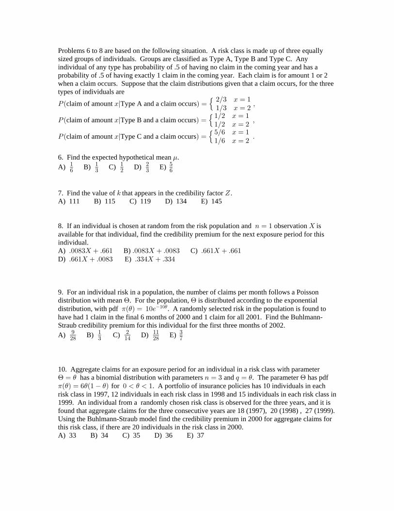
Problems 6 to 8 are based on the following situation. A risk class is made up of three equallysized groups of individuals. Groups are classified as Type A, Type B and Type C. Anyindividual of any type has probability of .5 of having no claim in the coming year and has aprobability of .5 of having exactly 1 claim in the coming year. Each claim is for amount 1 or 2when a claim occurs. Suppose that the claim distributions given that a claim occurs, for the threetypes of individuals are

TÐ Bl Ñ œ ß#Î$ B œ ""Î$ B œ #

claim of amount Type A and a claim occurs šTÐ Bl Ñ œ ß

"Î# B œ ""Î# B œ #

claim of amount Type B and a claim occurs šTÐ Bl Ñ œ Þ

&Î' B œ ""Î' B œ #

claim of amount Type C and a claim occurs š6. Find the expected hypothetical mean ..A) B) C) D) E)" " " # &

' $ # $ '

7. Find the value of that appears in the credibility factor .5 ^A) 111 B) 115 C) 119 D) 134 E) 145

8. If an individual is chosen at random from the risk population and observation is8 œ " \available for that individual, find the credibility premium for the next exposure period for thisindividual.A) B) C) Þ!!)$\ Þ''" Þ!!)$\ Þ!!)$ Þ''"\ Þ''"D) E) Þ''"\ Þ!!)$ Þ$$%\ Þ$$%

9. For an individual risk in a population, the number of claims per month follows a Poissondistribution with mean . For the population, is distributed according to the exponential@ @distribution, with pdf . A randomly selected risk in the population is found to1 )Ð Ñ œ "!/"!)

have had 1 claim in the final 6 months of 2000 and 1 claim for all 2001. Find the Buhlmann-Straub credibility premium for this individual for the first three months of 2002.A) B) C) D) E)* " # "" $

#) $ "% #) (

10. Aggregate claims for an exposure period for an individual in a risk class with parameter@ ) ) @œ 8 œ $ ; œ has a binomial distribution with parameters and . The parameter has pdf1 ) ) ) )Ð Ñ œ ' Ð" Ñ ! "for . A portfolio of insurance policies has 10 individuals in eachrisk class in 1997, 12 individuals in each risk class in 1998 and 15 individuals in each risk class in1999. An individual from a randomly chosen risk class is observed for the three years, and it isfound that aggregate claims for the three consecutive years are 18 (1997), 20 (1998) , 27 (1999).Using the Buhlmann-Straub model find the credibility premium in 2000 for aggregate claims forthis risk class, if there are 20 individuals in the risk class in 2000.A) 33 B) 34 C) 35 D) 36 E) 37

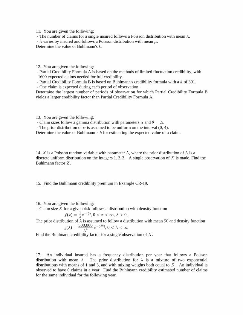
11. You are given the following: - The number of claims for a single insured follows a Poisson distribution with mean .- - varies by insured and follows a Poisson distribution with mean .- .Determine the value of Buhlmann's .5

12. You are given the following: - Partial Credibility Formula A is based on the methods of limited fluctuation credibility, with 1600 expected claims needed for full credibility. - Partial Credibility Formula B is based on Buhlmann's credibility formula with a of 391.5 - One claim is expected during each period of observation.Determine the largest number of periods of observation for which Partial Credibility Formula Byields a larger credibility factor than Partial Credibility Formula A.

13. You are given the following: - Claim sizes follow a gamma distribution with parameters and .α ) œ Þ& - The prior distribution of is assumed to be uniform on the interval (0, 4).αDetermine the value of Buhlmann’s for estimating the expected value of a claim.5

14. is a Poisson random variable with parameter , where the prior distribution of is a\ A Adiscrete uniform distribution on the integers 3 . A single observation of is made. Find the"ß #ß \Buhlmann factor .^

15. Find the Buhlmann credibility premium in Example CR-19.

16. You are given the following: - Claim size for a given risk follows a distribution with density function\

( ) , 0 , 010 B œ / B ∞ Þ- -ÐB- )

The prior distribution of is assumed to follow a distribution with mean 50 and density function-

( ) , 0500,0001 œ / ∞- --4

)Ð 100-

Find the Buhlmann credibility factor for a single observation of .\

17. An individual insured has a frequency distribution per year that follows a Poissondistribution with mean . The prior distribution for is a mixture of two exponential- -distributions with means of 1 and 3, and with mixing weights both equal to .5 . An individual isobserved to have 0 claims in a year. Find the Buhlmann credibility estimated number of claimsfor the same individual for the following year.

18. An individual insured has a frequency distribution per year that follows a Poissondistribution with mean . The prior distribution for is a mixture of two distributions.- -Distribution 1 is constant with value 1, and distribution 2 is exponential with a mean of 3, and themixing weights are both .5. An individual is observed to have 0 claims in a year. Find theBuhlmann credibility premium for the same individual for the following year.

19. The distribution of in three consecutive periods has the following characteristics:\IÒ\ Ó œ " ß Z +<Ò\ Ó œ " ß IÒ\ Ó œ # ß Z +<Ò\ Ó œ # ß IÒ\ Ó œ % ß" " # # $

G9@Ò\ ß\ Ó œ " ß G9@Ò\ ß\ Ó œ # ß G9@Ò\ ß\ Ó œ $ Þ" # " $ # $

Find the credibility premium for period 3 in terms of and using Buhlmann's credibility\ \" #

approach.A) B) C) # \ \ " #\ \ " \ #\" # " # " #

D) E) " #\ #\ " \ \" # " #

Problems 20 to 23 refer to the aggregate claim distribution per period with pdf\0ÐBl Ñ œ B/ B ! Ð Ñ œ !) ) @ 1 ) ) )# B # "

#) ) for , where has pdf e for .

20. Find the process variance.A) B) C) D) E) " # " # "

) ) ) ) )# # $

21. Find for G9@Ò\ ß\ Ó 3 Á 4 Þ3 4

A) B) C) D) E) " "% # " # %

22. Suppose that there are periods of claims. Find the value of coefficient that arises in the~8 α!

credibility premium.A) B) C) D) E) " # # " "

8# 8" 8# 8" #8"

23. Find the credibility factor if periods of claim information is available.^ 8

A) B) C) D) E) 8 8 8 8 #88# 8" #8# #8" #8"

24. An insurance company writes a book of business that contains several classes ofpolicyholders. You are given:(i) The average claim frequency for a policyholder over the entire book is 0.425.(ii) The variance of the hypothetical means is 0.370.(iii) The expected value of the process variance is 1.793.One class of policyholders is selected at random from the book. Nine policyholders are selected atrandom from this class and are observed to have produced a total of seven claims. Five additionalpolicyholders are selected at random from the same class. Determine the Buhlmann credibilityestimate for the total number of claims for these five policyholders.A) 2.5 B) 2.8 C) 3.0 D) 3.3 E) 3.9

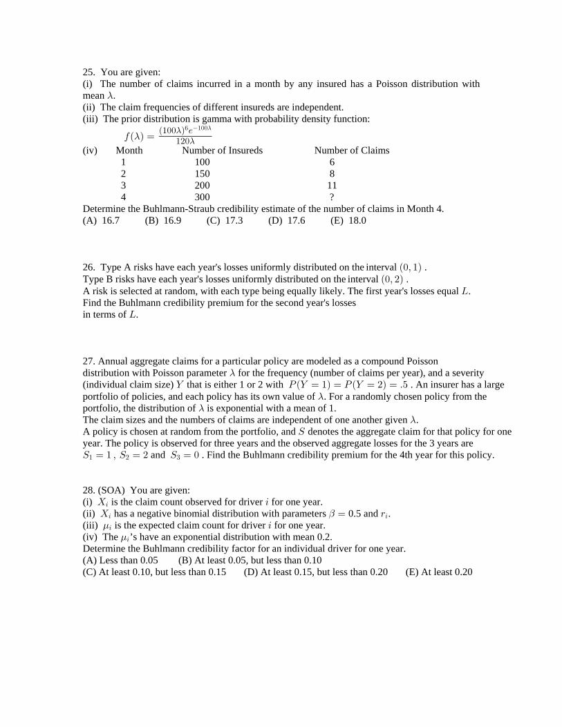
25. You are given:(i) The number of claims incurred in a month by any insured has a Poisson distribution withmean .-(ii) The claim frequencies of different insureds are independent.(iii) The prior distribution is gamma with probability density function:

0Ð Ñ œ-Ð"!! Ñ /

"#!-

-

' "!!-

(iv) Month Number of Insureds Number of Claims 1 100 6 2 150 8 3 200 11 4 300 ?Determine the Buhlmann-Straub credibility estimate of the number of claims in Month 4.(A) 16.7 (B) 16.9 (C) 17.3 (D) 17.6 (E) 18.0

26. Type A risks have each year's losses uniformly distributed on the interval .Ð!ß "ÑType B risks have each year's losses uniformly distributed on the interval .Ð!ß #ÑA risk is selected at random, with each type being equally likely. The first year's losses equal .PFind the Buhlmann credibility premium for the second year's lossesin terms of .P

27. Annual aggregate claims for a particular policy are modeled as a compound Poissondistribution with Poisson parameter for the frequency (number of claims per year), and a severity-(individual claim size) that is either 1 or 2 with . An insurer has a large] TÐ] œ "Ñ œ TÐ] œ #Ñ œ Þ&portfolio of policies, and each policy has its own value of . For a randomly chosen policy from the-portfolio, the distribution of is exponential with a mean of 1.-The claim sizes and the numbers of claims are independent of one another given .-A policy is chosen at random from the portfolio, and denotes the aggregate claim for that policy for oneWyear. The policy is observed for three years and the observed aggregate losses for the 3 years areW œ " ß W œ # W œ !" # $ and . Find the Buhlmann credibility premium for the 4th year for this policy.

28. (SOA) You are given:(i) is the claim count observed for driver for one year.\ 33

(ii) has a negative binomial distribution with parameters 0.5 and .\ œ <3 3"(iii) is the expected claim count for driver for one year..3 3(iv) The ’s have an exponential distribution with mean 0.2..3

Determine the Buhlmann credibility factor for an individual driver for one year.(A) Less than 0.05 (B) At least 0.05, but less than 0.10 (C) At least 0.10, but less than 0.15 (D) At least 0.15, but less than 0.20 (E) At least 0.20

29. For a portfolio of independent risks, the number of claims per period for a randomly chosenrisk has a Poisson distribution with a mean of , where has pdf , .@ @ ) ) )0Ð Ñ œ Ð5 "Ñ ! "5

Two risks are chosen at random and observed for one period, and it is found that Risk 1 has noclaims for the period and Risk 2 has 2 claims for the period. is the Buhlmann credibilityT"

premium for Risk 1 for the next period and is the Buhlmann credibility premium for Risk 2 forT#

the next period. Find .lim5Ä!

TT#

"

(A) (B) (C) (D) (E) ! " ∞$ && $

30. It is known that there are two groups of drivers in an insured population. One group has a 20percent accident probability per year and the other group has a 40 percent accident probability peryear. Two or more accidents per year per insured are not possible. The two groups compriseequal proportions of the population and each has the following accident severity distribution: Probability Size of Loss .80 100 .10 200 .10 400A merit rating plan is based on the pure premium experience of individual insureds for the prioryear. Calculate the credibility of an insured's experience.(A) Less than .01 (B) At least .01, but less than .02 (C) At least .02, but less than .03(D) At least .03, but less than .04 (E) At least .04

31. For a portfolio of independent risks, you are given:(i) The risks are divided into two classes, Class A and Class B.(ii) Equal numbers of risks are in Class A and Class B.(iii) For each risk, the probability of having exactly 1 claim during the year is 20% and theprobability of having 0 claims is 80%.(iv) All claims for Class A are of size 2.(v) All claims for Class B are of size , an unknown but fixed quantity.-One risk is chosen at random, and the total loss for one year for that risk is observed. You wish toestimate the expected loss for that same risk in the following year.Determine the limit of the Buhlmann credibility factor as goes to infinity.-(A) 0 (B) 1/9 (C) 4/5 (D) 8/9 (E) 1

32. The Buhlmann credibility factor based on exposures of a single risk is . Based on^ 8"$

8 " exposures, the Buhlmann credibility factor is . Find the Buhlmann credibility factor#&

based on exposures.8 #

(A) (B) (C) (D) (E) % & " ' &* "" # "" *

33. The Buhlmann credibility model is being applied to the loss variable (per exposure). It is\found that after exposures, the Buhlmann credibility factor is .8 œ &! ^ !Þ%How many additional exposures are needed to increase the factor to 0.5?^(A) 10 (B) 15 (C) 20 (D) 25 (E) 30

34. (SOA) You are given:(i) The claim count and claim size distributions for risks of type A are: Number of Claims Probabilities Claim Size Probabilities

0 4/9 500 1/31 4/9 1235 2/32 1/9

(ii) The claim count and claim size distributions for risks of type B are: Number of Claims Probabilities Claim Size Probabilities

0 1/9 250 2/31 4/9 328 1/32 4/9

(iii) Risks are equally likely to be type A or type B.(iv) Claim counts and claim sizes are independent within each risk type.(v) The variance of the total losses is 296,962.A randomly selected risk is observed to have total annual losses of 500.Determine the Buhlmann credibility premium for the next year for this same risk.¨(A) 493 (B) 500 (C) 510 (D) 513 (E) 514

35. (SOA) You are given the following information about a single risk:(i) The risk has exposures in each year.7(ii) The risk is observed for years.8(iii) The variance of the hypothetical means is .α(iv) The expected value of the annual process variance is A Þ

@7

Determine the limit of the Buhlmann-Straub credibility factor as approaches infinity.¨ 7

(A) (B) (C) (D) (E) 18 8 8 8

8 8 8 8 8 A+

A @ A@+ + +

#

(SOA) Use the following information for questions 36 and 37.You are given the following information about workers' compensation coverage:(i) The number of claims for an employee during the year follows a Poisson distribution with

mean , where is the salary (in thousands) for the employee."!! :

"!!:

(ii) The distribution of is uniform on the interval .: Ð!ß "!!Ó

36. An employee is selected at random. No claims were observed for this employee during theyear. Determine the posterior probability that the selected employee has salary greater than 50thousand.(A) 0.5 (B) 0.6 (C) 0.7 (D) 0.8 (E) 0.9

37. An employee is selected at random. During the last 4 years, the employee has had a total of 5claims. Determine the Buhlmann credibility estimate for the expected number of claims the¨employee will have next year.(A) 0.6 (B) 0.8 (C) 1.0 (D) 1.1 (E) 1.2

38. (SOA) You are given:(i) The full credibility standard is 100 expected claims.(ii) The square-root rule is used for partial credibility.You approximate the partial credibility formula with a Buhlmann credibility formula by selecting¨a Buhlmann value that matches the partial credibility formula when 25 claims are expected.¨ 5Determine the credibility factor for the Buhlmann credibility formula when 100 claims are¨expected.(A) 0.44 (B) 0.50 (C) 0.80 (D) 0.95 (E) 1.00

39. (SOA) You are given:(i) Claim size, , has mean and variance 500.\ .(ii) The random variable has a mean of 1000 and variance of 50..(iii) The following three claims were observed: 750, 1075, 2000Calculate the expected size of the next claim using Buhlmann credibility.(A) 1025 (B) 1063 (C) 1115 (D) 1181 (E) 1266

40. Losses for the year for a risk are uniformly distributed on , where is uniformlyÐ!ß Ñ) )distributed on the interval .Ð"ß #Ñ

The first year loss for a risk is . Find the Buhlmann credibility premium for the second year'sPloss for the same risk in terms of .P

41. Type A risks have each year's losses uniformly distributed on the interval .Ð!ß "ÑType B risks have each year's losses uniformly distributed on the interval .Ð!ß #ÑA risk is selected at random, with each type being equally likely. The first year's losses equal .PFind the Buhlmann credibility premium for the second year's lossesin terms of .P

A) C) D) E) Þ#!P Þ&" B) Þ#$P Þ&) Þ#&P Þ'" Þ#)P Þ&! Þ$!P Þ&&

42. The parameter has a prior distribution with pdf for .: Ð:Ñ œ #: ! : "1The model distribution is a discrete non-negative integer, and has a conditional distribution\given with probability function for : 0ÐBl:Ñ œ Ð" :Ñ : B œ !ß "ß #ß ÞÞÞB

(a) Find the marginal probability function of , for and find .\ 0ÐBÑ B œ !ß "ß #ß ÞÞÞ IÒ\Ó(b) Given a single observed , determine the posterior distribution of and identify its type.B :(c) Find the Bayesian premium IÒ\ l\ œ BÓ# "

(d) Apply Buhlmann's method to find the credibility premium.

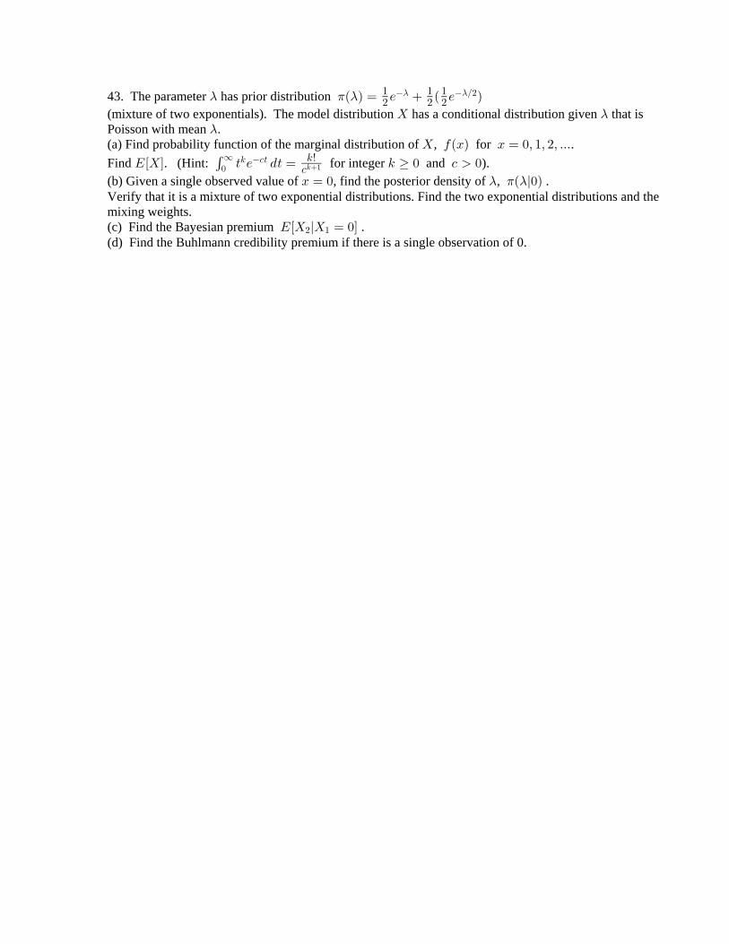
43. The parameter has prior distribution - 1 -Ð Ñ œ / Ð / Ñ" " "# # #

Î#- -

(mixture of two exponentials). The model distribution has a conditional distribution given that is\ -Poisson with mean .-(a) Find probability function of the marginal distribution of , for .\ 0ÐBÑ B œ !ß "ß #ß ÞÞÞ

Find . (Hint: for integer and ).IÒ\Ó > / .> œ 5   ! - !'!∞ 5 -> 5x

-5"

(b) Given a single observed value of , find the posterior density of , .B œ ! Ð l!Ñ- 1 -Verify that it is a mixture of two exponential distributions. Find the two exponential distributions and themixing weights.(c) Find the Bayesian premium .IÒ\ l\ œ !Ó# "

(d) Find the Buhlmann credibility premium if there is a single observation of 0.

CREDIBILITY - PROBLEM SET 6 SOLUTIONS

1. Hypothetical mean , Process variance .œ Ð Ñ œ IÒ\l Ó œ œ @Ð Ñ œ Z +<Ò\l Ó œ. - - - - - -IÒ\Ó œ œ IÒ Ð ÑÓ œ IÒ Ó œ Þ& Þ @ œ IÒ@Ð ÑÓ œ IÒ Ó œ Þ& ß. . A A A A

+ œ Z +<Ò Ð ÑÓ œ Z +<Ò Ó œ. A A ""#

(variance of the uniform distribution on interval is ).Ð+ß ,ÑÐ,+Ñ

"#

#

^ œ œ œ8 8 88 8'8

@+

"Î#"Î"#

. Answer: C

2. This is a standard Bayesian analysis. The formal algebraic explanation is more long-windedthan the calculations needed.T Ò ∩ Ó(urn A is chosen) (sum of two balls is 1)œ TÒ l Ó † T Ò Ósum of two balls is 1 urn A is chosen urn A is chosen

balls are or urn A is chosenœ TÒ !ß " "ß ! l Ó † œ Ò#ÐÞ#ÑÐÞ)ÑÓ † œ Þ"' Þ" "# #

Similarly, (urn B is chosen) (sum of two balls is 1)T<Ò ∩ Ó œ Ò#ÐÞ(ÑÐÞ$ÑÓ † œ Þ#" Þ"#

Then sum of two balls is 1T Ò Óœ T Ò ∩ Ó(urn A is chosen) (sum of two balls is 1)

(urn B is chosen) (sum of two balls is 1) . TÒ ∩ Ó œ Þ"' Þ#" œ Þ$(We can find conditional (posterior) probabilities of urn chosen given sum of balls:T Ò l Ó œurn A is chosen sum of two balls is 1 T Ò ∩ Ó

T Ò Ó(urn A is chosen) (sum of two balls is 1)

sum of two balls is 1œ œÞ"' Þ"'

Þ"'Þ#" Þ$( , and similarlyT Ò l Ó œ œurn B is chosen sum of two balls is 1 .Þ#" Þ#"

Þ"'Þ#" Þ$(The expected value on a ball if chosen from urn A is ,Ð!ÑÐÞ#Ñ Ð"ÑÐÞ)Ñ œ Þ)and the expected value on a ball if chosen from urn B is 7 3Ð!ÑÐÞ Ñ Ð"ÑÐÞ Ñ œ Þ$ ÞUsing the posterior probabilities for urns A and B, we can find the conditional expected value ona ball chosen from the same urn as the first two balls - this conditional expectation isIÒ l Ó 3rd ball value sum of first two balls is 1 œ IÒ l Ó † T Ò l Óball value urn A urn A sum of first two balls is 1 IÒ l Ó † T Ò l Óball value urn B urn B sum of first two balls is 1 œ ÐÞ)ÑÐ Ñ ÐÞ$ÑÐ Ñ œ Þ&"' Þ"' #"

$( $(The expected value of the sum of two more balls under these circumstances would be ."Þ!$#

Another way to describe these calculations is the following. We know the expected value of thesum of two balls if urn A is chosen (1.6) and also if urn B is chosen (.6). If we had no priorinformation about the sum of the first two balls, then the expected value of the sum of two ballsfrom a randomly chosen urn would beIÒ l Ó † T Ò Ó IÒ l Ó † T Ò Ó œ Ð"Þ'Ñ ÐÞ'Ñ œ "Þ"sum urn A urn A sum urn B urn B ." "

# #Although each of urns A and B have the same chance of being chosen initially, we now haveadditional information about which urn might have been chosen. We use Bayesian analysis tofind the probability that the urn was A (or B) given that the two balls chosen from the unknownurn added up to 1. These conditional probabilities were found to beT Ò l Ó œ T Ò l Ó œA sum is 1 and B sum is 1 . We use these Bayesian updated probabilities"' #"

$( $(to find the expected sum of the next two balls.

2. continuedIÒ l Ó † T Ò l Ósum urn A urn A sum of first 2 balls is 1IÒ l Ó † T Ò l Ó œ Ð"Þ'Ñ ÐÞ'Ñ œ "Þ!$# Þsum urn B urn B sum of first 2 balls is 1 "' #"

$( $(In this last formulation, we have replaced urn A withT Ò ÓT Ò l Óurn A sum of first 2 balls is 1 , and similarly for B.

Note that we could have found the conditional probabilities of the next ball being either 0 or 1given that the sum of the first two balls was 1 -T Ò l Ónext ball is 0 sum of first two balls is 1œ TÒ l ∩ Ó † T Ò l Óball is 0 (urn A) (sum of first two balls is 1) urn A sum of first two balls is 1 TÒ l ∩ Ó † T Ò l Óball is 0 (urn B) (sum of first two balls is 1) urn B sum of first two balls is 1œ ÐÞ#ÑÐ Ñ ÐÞ(ÑÐ Ñ œ"' #" "(Þ*

$( $( $( .Algebraically, this relationship isT Ò l Ó œnext ball is 0 sum of first two balls is 1 T Ò!∩ Ó

T Ò ÓÓ(sum is 1)

sum is 1

œ TÒ!∩ ∩ Ó T Ò!∩ ∩ Ó

T Ò ÓÓ T Ò ÓÓA (sum is 1) B (sum is 1)sum is 1 sum is 1

œ † †T Ò!∩ ∩ Ó T Ò ∩ Ó T Ò!∩ ∩ Ó T Ò ∩ ÓT Ò ∩ ÓÓ T Ò ÓÓ T Ò ∩ ÓÓ T Ò ÓÓ

A (sum is 1) A (sum is 1) B (sum is 1) B (sum is 1)A sum is 1 sum is 1 B sum is 1 sum is 1

œ TÒ l ∩ Ó † T Ò l Óball is 0 (urn A) (sum of first two balls is 1) urn A sum of first two balls is 1 TÒ l ∩ Ó † T Ò l Óball is 0 (urn B) (sum of first two balls is 1) urn B sum of first two balls is 1 .In a similar way, next ball is 1 sum of first two balls is 1T Ò l Ó œ Þ"*Þ"

$(

The comments that were made above regarding the expectation apply to probabilities as well.The probability of choosing a 0 from urn A is .2, and the probability of choosing a 0 from urn Bis .7. If we had no information about the sum of the first two balls, then each of urns A and Bhave a chance of being chosen, and the probability of choosing a 0"

#

from a randomly chosen urn would be , and the probability of choosing a 1ÐÞ#Ñ ÐÞ(Ñ œ Þ%&" "# #

from a randomly chosen urn would be The Bayesian analysis above gaveÐÞ)Ñ ÐÞ$Ñ œ Þ&& Þ" "# #

us the conditional probabilities of choosing urn A or urn B given that the first two balls had a sumof 1 - A sum is 1 and B sum is 1 .T Ò l Ó œ T Ò l Ó œ"' #"

$( $(We use these Bayesian updated probabilities (instead of ) to find the probability of choosing a 0"

#

or a 1 given that the sum of the first two balls was 1 -T Ò l Ó œ ÐÞ#Ñ ÐÞ(Ñ œ ßnext ball is 0 sum of first two balls is 1 and"' #" "(Þ*

$( $( $(

T Ò l Ó œ ÐÞ)Ñ ÐÞ$Ñ œ Þnext ball is 1 sum of first two balls is 1 "' #" "*Þ"$( $( $(

Then ball value sum of first two balls is 1 ( ) (1)( ) ,IÒ l Ó œ Ð!Ñ œ œ Þ&"'"(Þ* "*Þ" "*Þ"$( $( $(

as before. The two conditional probabilitiesT Ò l Ó œnext ball is 0 sum of first two balls is 1 and"(Þ*

$(

T Ò l Ó œnext ball is 1 sum of first two balls is 1 form the posterior distribution of the value of"*Þ"$(

the next ball chosen (from the same urn) given that the sum of the first 2 balls was 1. Answer: C

3. We now put this situation in the context of the Buhlmann credibility approach. The parameter

@ @ describes the urn chosen: To find the Buhlmann credibility estimateA prob. B prob.

œ Þš "#"#

(premium) for the sum of the next two balls we must identify the random variable , and the\conditional distribution of given . In this case, is the number on a ball chosen from an\ \@urn.

The conditional distribution of given A is A with, , \ œ 0ÐBl œ Ñ œ ß

Þ# B œ !Þ) B œ "

@ @ šIÒ\l Ó œ Þ) 0ÐBl œ Ñ œ IÒ\l Ó œ Þ$

Þ( B œ !Þ$ B œ "

A , and B , with B (these conditional@ šexpectations were found in Problem 2).

The credibility premium is , where^\ Ð" ^Ñ ^ œ œ Þ

. 8 885 8@

+

3. continuedThe values of the various components are found as follows.

The hypothetical mean and its expected value (the collective or pure premium). . @œ IÒ Ð ÑÓ œ IÒ\Ó \ - since, in the marginal distribution of , there is chance of choosing"

#

urn A or urn B, we have A B .IÒ\Ó œ IÒ\l Ó † IÒ\l Ó † œ ÐÞ)ÑÐ Ñ ÐÞ$ÑÐ Ñ œ Þ&&" " " "# # # #

Note that the hypothetical mean is , which in this case is. ) @ )Ð Ñ œ IÒ\l œ Ó. @ . @Ð Ñ œ IÒ\l œ Ó œ IÒ\l Ó œ Þ) Ð Ñ œ IÒ\l œ Ó œ IÒ\l Ó œ Þ$A A A , and B B B , and then. . @ . @ . @œ IÒ Ð ÑÓ œ Ð Ñ † T Ò œ Ó Ð Ñ † T Ò œ Ó œ ÐÞ)ÑÐ Ñ ÐÞ$ÑÐ Ñ œ Þ&&A A B B ," "

# #as before.

The process variance, and its expected value@ œ IÒZ +<Ð\ l ÑÓ œ IÒ@Ð ÑÓ , where3 @ @Z +<Ò\l œ Ó œ IÒ\ l œ Ó ÐIÒ\l œ ÓÑ œ IÒ\ l œ Ó ÐÞ)Ñ@ @ @ @A A A A ,# # # #

and since A weIÒ\ l œ Ó œ Ð! ÑÐÞ#Ñ Ð" ÑÐÞ)Ñ œ Þ) ß# # #@have A A , and similarly,@Ð Ñ œ Z +<Ò\l œ Ó œ Þ) Þ'% œ Þ"'@@Ð Ñ œ Z +<Ò\l œ Ó œ Þ$ ÐÞ$Ñ œ Þ#" ÞB B Then,@ #

@ œ IÒ@Ð ÑÓ œ @Ð Ñ † T Ò œ Ó @Ð Ñ † T Ò œ Ó œ ÐÞ"'ÑÐ Ñ ÐÞ#"ÑÐ Ñ œ Þ")&@ @ @A A B B ." "# #

The variance of the hypothetical mean+ œ Z +<Ò IÐ\ l œ ÑÓ œ Z +<Ò Ð ÑÓ œ IÒ Ð Ñ Ó ÐIÒ Ð ÑÓÑ 3

# #@ ) . @ . @ . @œ Ð Ñ † T Ò œ Ó Ð Ñ † T Ò œ Ó ÐÞ&&Ñ. @ . @A A B B# # #

œ ÐÞ)Ñ Ð Ñ ÐÞ$Ñ Ð Ñ Þ$!#& œ Þ!'#& Þ# #" "# #

There are observations, so that .8 œ # \ œ œ Þ& \ \

#" #

Also, so that , and5 œ œ œ #Þ*' ß ^ œ œ œ Þ%!$#@+

Þ")& 8 #Þ!'#& 85 ##Þ*'

the credibility premium is per^\ Ð" ^Ñ œ ÐÞ%!$#ÑÐÞ&Ñ ÐÞ&*')ÑÐÞ&&Ñ œ Þ&#*)

.new ball chosen. There will be two balls chosen, so the expected total of the next two balls (thecredibility premium for two more claims) is Answer: C#ÐÞ&#*)Ñ œ "Þ!' Þ

4. The solution requires a Bayesian analysis similar to that in Problem 7 above.We find unconditional probabilities:T ÒE ∩ ! ! Ó( claims in first period and claims in second period)œ TÒ! ! lEÓ † T ÒEÓ œ ÐÞ)ÑÐÞ)ÑÐÞ&Ñ œ Þ$# claims in first period and claims in second periodT ÒF ∩ Ð!ß !ÑÓ œ ÐÞ'ÑÐÞ'ÑÐÞ&Ñ œ Þ") p T Ò!ß !Ó œ Þ$# Þ") œ Þ& (this is the unconditionalprobability of no claims in either of two periods for a randomly chosen risk)ÞWe now find conditional probabilities:T ÒEl!ß !Ó œ œ œ Þ'% T ÒFl!ß !Ó œ œ œ Þ$' Þ

T ÒE∩Ð!ß!ÑÓ T ÒF∩Ð!ß!ÑÓT Ò!ß!Ó Þ& T Ò!ß!Ó Þ&

Þ$# Þ"), and The conditional expectation of aggregate claims per period for each risk:IÒ\lEÓ œ Ð!ÑÐÞ)Ñ Ð&!ÑÐÞ"'Ñ Ð"!!!ÑÐÞ!%Ñ œ %) ,IÒ\lFÓ œ Ð!ÑÐÞ'Ñ Ð&!ÑÐÞ#%Ñ Ð"!!!ÑÐÞ"'Ñ œ "(# ÞThe conditional expected aggregate claims per period given no claims in first two periods isfound using the updated (Bayesian) probabilities of and :E FIÒ\l!ß !Ó œ IÒ\lEÓ † T ÒEl!ß !Ó IÒ\lFÓ † T ÒFl!ß !Ó œ Ð%)ÑÐÞ'%Ñ Ð"(#ÑÐÞ$'Ñ œ *#Þ'% Þ Answer: E

5. The collective premium is ;. . @œ IÒ\Ó œ IÒ Ð ÑÓ œ Ð%)ÑÐ Ñ Ð"(#ÑÐ Ñ œ ""!" "# #

in this case, is either risk A or risk B, each with prob. .5, and the hypothetical means are@. .ÐEÑ œ %) ß ÐFÑ œ "(#. The process variances for risks A and B are@ÐEÑ œ Z +<Ò\l œ EÓ œ Ð! ÑÐÞ)Ñ Ð&! ÑÐÞ"'Ñ Ð"!!! ÑÐÞ!%Ñ Ð%)Ñ œ $)ß !*' ß@ # # # #

@ÐFÑ œ Z +<Ò\l œ FÓ œ Ð! ÑÐÞ'Ñ Ð&! ÑÐÞ#%Ñ Ð"!!! ÑÐÞ"'Ñ Ð"(#Ñ œ "$"ß !"' ß@ # # # #

and the expected process variance is @ œ IÒ@Ð ÑÓ œ Ð$)ß !*' "$"ß !"'Ñ œ )%ß &&' Þ@ "#

The variance of the hypothetical mean is+ œ Z +<Ò Ð ÑÓ œ Ð%) ÑÐ Ñ Ð"(# ÑÐ Ñ ""! œ $)%% Þ. @ # # #" "

# #

The credibility factor is Since there are no claims in each of the^ œ œ œ Þ8 # "8 "##

@+

)%ß&&'$)%%

first two periods, , so that .\ œ \ œ ! \ œ !

" #

The credibility premium is then ^\ Ð" ^Ñ œ Ð ÑÐ!Ñ Ð ÑÐ""!Ñ œ "!!Þ)$ Þ

. " """# "#

Notice the strong similarity between Problems 2,3 and 4,5. Urn becomes risk, and number onball becomes aggregate claim for one exposure period. Otherwise, the analysis is the same. Answer: E

6. each with probability , and@ œ "ß #ß $ "$

. ) @ ) . @Ð Ñ œ IÒ\l œ Ó Ð"Ñ œ IÒ\l œ "Ó œ ÐÞ&ÑÒ" † # † Ó œ ß : # " #$ $ $

. @ . @Ð#Ñ œ IÒ\l œ #Ó œ ß Ð$Ñ œ IÒ\l œ $Ó œ Þ$ (% "#

Therefore Answer: D. . @œ IÒ Ð ÑÓ œ Ð ÑÒ Ó œ Þ" # $ ( #$ $ % "# $

7. .@Ð Ñ œ Z +<Ò\l œ Ó) @ )

0 ÐBl œ "Ñ œ

B œ !

† œ B œ "

† œ B œ #

\l@ ) œ"#" # "# $ $" " "# $ '

p @Ð"Ñ œ Ð!Ñ Ð Ñ Ð"Ñ Ð Ñ Ð#Ñ Ð Ñ ÐIÒ\l œ "ÓÑ œ " Ð Ñ œ ,# # # # #" " " # &# $ & $ *@

0 ÐBl œ #Ñ œ ß p @Ð#Ñ œ Ð Ñ œ

B œ !

B œ "

B œ #

\l#

@ ) œ"#"%"%

& $ ""% % "' , and

0 ÐBl œ $Ñ œ p @Ð$Ñ œ Ð Ñ œ

B œ !

B œ "

B œ #

\l#

@ ) œ"#&"#""#

$ ( &*% "# "%% .

Then @ œ IÒ@Ð ÑÓ œ Ð ÑÐ Ñ Ð ÑÐ Ñ Ð ÑÐ Ñ œ Þ@ & " "" " &* " #$)* $ "' $ "%% $ %$#

Also, + œ Z +<Ò Ð ÑÓ œ IÒ Ð Ñ Ó ÐIÒ Ð ÑÓÑ. @ . @ . @# #

œ Ð Ñ Ð Ñ Ð Ñ Ð Ñ Ð Ñ Ð Ñ Ð Ñ œ Þ# " $ " ( " # #$ $ % $ "# $ $ %$#

# # # #

Then . Answer: C5 œ œ œ ""*@ #$)+ #

8. The credibility premium is ^\ Ð" ^Ñ Þ

.

In this case, and so that , and8 œ " 5 œ ""* ^ œ œ Þ!!)$""""*

\ œ \ œ . From Problem 6, we have . The credibility premium is. #

$

ÐÞ!!)$Ñ\ ÐÞ**"(ÑÐ Ñ œ Þ!!)$\ Þ''" Þ#$ Answer: A

9. Let represent the number of claims in a month for a randomly chosen individual. ThenG. ) @ ) ) )Ð Ñ œ IÒG l œ Ó œ3 (mean of the Poisson distribution with parameter ),. . @ @œ IÒGÓ œ IÒ Ð ÑÓ œ IÒ Ó œ Þ" (mean of the exponential),@Ð Ñ œ Z +<ÒGl œ Ó œ) @ ) ) )(variance of the Poisson distribution with parameter ),@ œ IÒ@Ð ÑÓ œ IÒ Ó œ Þ" + œ Z +<Ò Ð ÑÓ œ Z +<Ò Ó œ Þ!"@ @ . @ @, and (variance of the exponential isthe square of the mean).

Let denote the number of claims in each of the final 6 months of 2000 for theG ßG ß ÞÞÞß G"ß" "ß# "ß'

individual, and let denote the number of claims in each of the 12 months ofG ßG ß ÞÞÞß G#ß" #ß# # ß"#

2001. We have 18 monthly claim numbers and we can apply the Buhlmann method to .7 œ G

5 œ œ œ "! ß ^ œ œ œ@ Þ" 7 ") ")+ Þ!" 75 ")"! #) ,

and .G œ œ G G âG G G âÞG

") ")#"ß" "ß# "ß' #ß" #ß# # ß"#

Then the Buhlmann(-Straub) credibility premium is^G Ð" ^Ñ œ Ð ÑÐ Ñ Ð ÑÐÞ"Ñ œ

. ") # "! $#) ") #) #) per month.

The credibility premium for the first three months of 2001 is Answer: A$Ð Ñ œ Þ$ *#) #)

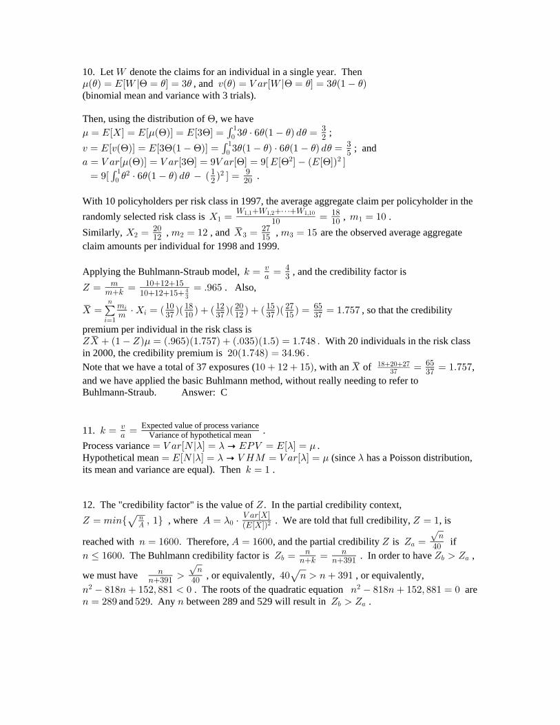
10. Let denote the claims for an individual in a single year. Then[. ) @ ) ) ) @ ) ) )Ð Ñ œ IÒ[ l œ Ó œ $ @Ð Ñ œ Z +<Ò[ l œ Ó œ $ Ð" Ñ, and (binomial mean and variance with 3 trials).

Then, using the distribution of , we have@

. . @ @ ) ) ) )œ IÒ\Ó œ IÒ Ð ÑÓ œ IÒ$ Ó œ $ † ' Ð" Ñ . œ'!" $

# ;@ œ IÒ@Ð ÑÓ œ IÒ$ Ð" ÑÓ œ $ Ð" Ñ † ' Ð" Ñ . œ@ @ @ ) ) ) ) )'

!" $

& ; and+ œ Z +<Ò Ð ÑÓ œ Z +<Ò$ Ó œ *Z +<Ò Ó œ *ÒIÒ Ó ÐIÒ ÓÑ Ó. @ @ @ @ @# #

œ *Ò † ' Ð" Ñ . Ð Ñ Ó œ'!" # #) ) ) ) " *

# #! .

With 10 policyholders per risk class in 1997, the average aggregate claim per policyholder in therandomly selected risk class is , .\ œ œ 7 œ "!" "

[ [ â["! "!

")"ß" "ß# "ß"!

Similarly, , , and , are the observed average aggregate\ œ 7 œ "# \ œ 7 œ "&

# # $ $#! #("# "&

claim amounts per individual for 1998 and 1999.

Applying the Buhlmann-Straub model, , and the credibility factor is5 œ œ@ %+ $

^ œ œ œ Þ*'&7 "!"#"&75 "!"#"&%

$

. Also,

\ œ † \ œ Ð ÑÐ Ñ Ð ÑÐ Ñ Ð ÑÐ Ñ œ œ "Þ(&(

3œ"

8

377 $( "! $( "# $( "& $(

"! ") "# #! "& #( '&3 , so that the credibility

premium per individual in the risk class is^\ Ð" ^Ñ œ ÐÞ*'&ÑÐ"Þ(&(Ñ ÐÞ!$&ÑÐ"Þ&Ñ œ "Þ(%) Þ

. With 20 individuals in the risk classin 2000, the credibility premium is #!Ð"Þ(%)Ñ œ $%Þ*' Þ

Note that we have a total of 37 exposures ( , with an of ,"! "# "&Ñ \ œ œ "Þ(&( ")#!#(

$('&$(

and we have applied the basic Buhlmann method, without really needing to refer toBuhlmann-Straub. Answer: C

11. 5 œ œ@+

Expected value of process varianceVariance of hypothetical mean .

Process variance .œ Z +<ÒRl Ó œ p ITZ œ IÒ Ó œ- - - .Hypothetical mean (since has a Poisson distribution,œ IÒRl Ó œ p Z LQ œ Z +<Ò Ó œ- - - . -its mean and variance are equal). Then . 5 œ "

12. The "credibility factor" is the value of . In the partial credibility context,^

^ œ 738Ö ß "× E œ † ^ œ "È 8E ! , where . We are told that full credibility, , is-

Z +<Ò\ÓÐIÒ\ÓÑ#

reached with Therefore, , and the partial credibility is if8 œ "'!!Þ E œ "'!! ^ ^ œ+

È8

%!8 Ÿ "'!! ^ œ œ ^ ^. The Buhlmann credibility factor is . In order to have ,, , +

8 885 8$*"

we must have , or equivalently, , or equivalently,88$*" %!

8 %! 8 8 $*"

È È8 )")8 "&#ß ))" ! 8 )")8 "&#ß ))" œ !# # . The roots of the quadratic equation are8 œ #)* &#* 8 ^ ^and . Any between 289 and 529 will result in ., +

13. The hypothetical mean given is , and the variance of the hypothetical mean isα )α αœ Þ&

Z LQ œ Z +<ÐÞ& Ñ œ Þ#&Z +<Ð Ñ œ ÐÞ#&ÑÐ Ñ œ œ +α α % ""# $

#

.The process variance is , the variance of the gamma distribution, which isTZ œ Z +<Ò\l Óα) α α# œ Þ#& , and the expected value of the process variance isITZ œ IÒÞ#& Ó œ ÐÞ#&ÑÐ#Ñ œ Þ& œ @ 5 œ œ œ "Þ&α . Then .@

+ "Î$"Î#

14. , . A A A A A AÐ Ñ œ IÒ\l Ó œ @Ð Ñ œ Z +<Ò\l Ó œ ß

. . A Aœ IÒ Ð ÑÓ œ IÒ Ó œ Ð ÑÐ" # $Ñ œ #"$ .

+ œ Z +<Ò Ð ÑÓ œ Z +<Ò Ó œ Ð ÑÐ" # $ Ñ # œ. A A " #$ $

# # # # .@ œ IÒ@Ð ÑÓ œ IÒ Ó œ #A A .8 œ " \ ^ œ œ œ(one observation of ), so .8 " "

8 %"@+

##Î$

15. has an exponential distribution, and is uniformly distributed on .\l Ò"!ß #!Ó) @. ) ) ) ) ) )Ð Ñ œ IÒ\l Ó œ ß @Ð Ñ œ Z +<Ò\l Ó œ # .. . ) ) . ) )œ IÒ Ð ÑÓ œ IÒ Ó œ œ "& + œ Z +<Ò Ð ÑÓ œ Z +<Ò Ó œ œ )Þ$$$"!#!

# "#Ð#!"!Ñ , ,

#

@ œ IÒ@Ð ÑÓ œ IÒ Ó œ ÐÞ"Ñ . œ #$$Þ$$) ) ) )# #"!

#!' .For data points, the Buhlmann credibility factor is .8 œ ) ^ œ œ œ Þ###) )

) )@+

#$$Þ$$)Þ$$$

For the data points , with , the Buhlmann8 œ ) $ ß % ß ) ß "! ß "# ß ") ß ## ß $& \ œ "%

credibility premium is .ÐÞ###ÑÐ"%Ñ ÐÞ(()ÑÐ"&Ñ œ "%Þ()

16. has an exponential distribution, and has an inverse gamma distribution\l- -with . and .α ) . - - - - - -œ $ ß œ "!! Ð Ñ œ IÒ\l Ó œ @Ð Ñ œ Z +<Ò\l Ó œ #

@ œ IÒ@Ð ÑÓ œ IÒ Ó œ œ &!!!- -# )α α

#

Ð "ÑÐ #Ñ .

+ œ Z +<Ò Ð ÑÓ œ Z +<Ò Ó œ IÒ Ó ÐIÒ ÓÑ œ &!!! Ð Ñ œ #&!!. - - - -# # #)α" .

^ œ œ œ" " "" $"@

+&!!!#&!!

.

17. . Since is a mixture, IÒ\l Ó œ ß Z +<Ò\l Ó œ IÒ Ó œ ÐÞ&ÑÐ"Ñ ÐÞ&ÑÐ$Ñ œ #- - - - - -and (each component of the mixture has anIÒ Ó œ ÐÞ&ÑÐ# ‚ " Ñ ÐÞ&ÑÐ# ‚ $ Ñ œ "!-# # #

exponential distribution, and the second moment of an exponential is two times the square of themean). Then . . - - - -œ IÒ Ð ÑÓ œ IÒ Ó œ # ß @ œ IÒ@Ð ÑÓ œ IÒ Ó œ # ß+ œ Z +<Ò Ð ÑÓ œ Z +<Ò Ó œ IÒ Ó ÐIÒ ÓÑ œ '. - - - -# # .For a single observation of , , the Buhlmann credibility factor is .\ 8 œ " ^ œ œ" $

" %#'

With , the Buhlmann credibility estimate for the next year is\ œ !

^\ Ð" ^Ñ œ ! Ð ÑÐ#Ñ œ

. " "% # .

18. . Since is a mixture, IÒ\l Ó œ ß Z +<Ò\l Ó œ IÒ Ó œ ÐÞ&ÑÐ"Ñ ÐÞ&ÑÐ$Ñ œ #- - - - - -and (the first component is constant at 1). ThenIÒ Ó œ ÐÞ&ÑÐ"Ñ ÐÞ&ÑÐ# ‚ $ Ñ œ *Þ&-# #

. . - - - -œ IÒ Ð ÑÓ œ IÒ Ó œ # ß @ œ IÒ@Ð ÑÓ œ IÒ Ó œ # ß+ œ Z +<Ò Ð ÑÓ œ Z +<Ò Ó œ IÒ Ó ÐIÒ ÓÑ œ &Þ&. - - - -# # .For a single observation of , , the Buhlmann credibility factor is .\ 8 œ " ^ œ œ Þ($$"

" #&Þ&

With , the Buhlmann credibility estimate for the next year is\ œ !^\ Ð" ^Ñ œ ! ÐÞ#'(ÑÐ#Ñ œ Þ&$%

. .

19. According to Buhlmann's approach, we solve the normal equations for the -coefficients: ~αIÒ\ Ó œ IÒ\ Ó IÒ\ Ó$ ! " " # #α α α~ ~ ~ ~ ~G9@Ò\ ß\ Ó œ Z +<Ò\ Ó G9@Ò\ ß\ Ó" $ " " # " #α α .~ ~G9@Ò\ ß\ Ó œ G9@Ò\ ß\ Ó Z +<Ò\ Ó# $ " # " # #α αSubstituting the given values, these equation become ~ ~ ~% œ #α α α! " #

~ ~# œ α α" #

~ ~$ œ #α α" #

with solution . The credibility premium is~ ~ ~α α α! " #œ " ß œ " ß œ "

α α~ ~ , with . Answer: E! 3 3 " #3œ"

8

\ œ " \ \ 8 œ #

20. @Ð Ñ œ Z +<Ò\l œ Ó œ IÒ\ l œ Ó ÐIÒ\l œ ÓÑ) @ ) @ ) @ )# #

œ B † B/ .B Ð B † B/ .BÑ œ Ð Ñ œ Þ' '! !

∞ ∞# # B # B # #) )) ) ' # #) ) )# # Answer: D

21. This model satisfies the requirements of Buhlmann's model (common mean, variance andcovariances for the 's). .\ G9@Ò\ ß\ Ó œ + œ Z +<Ò Ð ÑÓ4 3 4 . @

From Problem 20 above , so that. ) @ )Ð Ñ œ IÒ\l œ Ó œ #)

Z +<Ò Ð ÑÓ œ Z +<Ò Ó œ IÒÐ Ñ Ó ÐIÒ ÓÑ. @ # # #@ @ @

# #

e e Answer: Cœ † . Ð † . Ñ œ # Ð"Ñ œ " Þ' '! !

∞ ∞# # # #% " # "# #) )# ) ) ) )) )

22. , where and (from Problem 21),~α . . @! œ + œ " ß œ IÒ Ð ÑÓ œ IÒ Ó œ "@

8+@#.@

and e (from Problem 20).@ œ IÒ@Ð ÑÓ œ IÒ Ó œ † . œ "@ ) )# # "#@ )# #

'!

∞ # )

Thus, (in fact, all ). Answer: D~ ~α α! 4œ œ" "8" 8"

23. Answer: B^ œ œ œ Þ8 8 885 8 8"@

+

24. The Buhlmann credibility factor is , and the Buhlmann credibility estimate is^ œ8

8@+

^\ Ð" ^Ñ œ Þ%#& ß + œ Þ$(! @ œ "Þ(*$ 8 œ *

. . . We are given and . For the policyholders, the sample mean for number of claims is . The credibility factor is\ œ

(*

^ œ œ Þ'&!*

*"Þ(*$Þ$(!

. The Buhlmann credibility estimate for number of claims for another

policyholder of the same class is . The credibility estimate forÐÞ'&ÑÐ Ñ ÐÞ$&ÑÐÞ%#&Ñ œ Þ'&%$(*

5 policyholders of the same class is . Answer: DÐ&ÑÐÞ'&%$Ñ œ $Þ#(

25. This is a combination of a gamma prior distribution and Poisson model distribution. For thiscombination, the Buhlmann credibility premium is the same as the Bayesian credibility premiumestimate (called exact credibility). The Buhlmann-Straub estimate in this case is the same as theBuhlmann estimate (which is the same as the Bayesian estimate). The first three months of dataare combined so that we have a total of insureds with a total number of claims of8 œ %&!

3œ"

%&!

3B œ ' ) "" œ #& . Using the Bayesian method, the predictive mean for the next policy of

the same type is (actually, the predictive distribution for the number ofÐ B ÑÐ Ñα D 3))8 "

claims on the next policy of the same type is a negative binomial distribution with parameters< œ B œα D "3 and ).)

)8 "

In this problem where and are the gamma parameters from the priorα )œ ' œ œ Þ!"""!!

distribution. Therefore, and .< œ ' #& œ $" œ œ Þ!!")")"Þ!"

Ð%&!ÑÐÞ!"Ñ"

The predictive expectation is , This is the expected number of claims for a single< œ Þ!&'$'"insured in Month 4. For 300 insureds in Month 4 we would expect .Ð$!!ÑÐÞ!&'$'Ñ œ "'Þ*If this had not involved the specific combination of the gamma prior and Poisson modeldistributions we would have had to use the Buhlmann method.

Note that we are implicitly assuming that all 450 insureds have the same (unknown) , and we-wish to find the expected number of claims from 300 more policies with the same . That is the-standard Bayesian approach. Answer: B

26. Prior distribution is TÐEÑ œ TÐFÑ œ Þ"#

Hypothetical means are .. .ÐEÑ œ IÒ\lEÓ œ Þ& ß ÐFÑ œ IÒ\lFÓ œ "

Process variances are .@ÐEÑ œ Z +<Ò\lEÓ œ ß @ÐFÑ œ œ" % ""# "# $

. œ IÒ\Ó œ œ ÐÞ&Ñ Ð"Ñ œexpected hypothetical mean .Ð Ñ Ð Ñ" " $# # %

@ œ œ œexpected process variance .Ð ÑÐ Ñ Ð ÑÐ Ñ" " " " &"# # $ # #%

+ œ œ Ð" Þ&Ñ œvariance of hypothetical mean .#Ð ÑÐ Ñ" " "# # "'

^ œ œ œ Þ#$!)88@

+

"

"&Î#%"Î"'

.

Buhlmann credibility premium is^P Ð" ^Ñ œ Þ#$!)P Þ('*# œ Þ#$!)P Þ&('*. Ð Ñ$% .

27. Hypothetical mean is IÐWl Ñ œ † IÐ] Ñ œ "Þ& Þ- - -Process variance is .Z +<ÐWl Ñ œ † IÐ] Ñ œ #Þ&- - -#

Expected hypothetical mean is .. - -œ IÐIÐWl ÑÑ œ IÐ"Þ& Ñ œ "Þ&Expected process variance is .@ œ IÐZ +<ÐWl ÑÑ œ IÐ#Þ& Ñ œ #Þ&- -Variance of hypothetical mean is .+ œ Z +<ÐIÐWl ÑÑ œ Z +<Ð"Þ& Ñ œ #Þ#&- -

^ œ œ œ Þ(#*( Þ$ $$ $@

+#Þ&#Þ#&

Buhlmann credibility premium is .^W Ð" ^Ñ œ ÐÞ(#*(Ñ ÐÞ#(!$ÑÐ"Þ&Ñ œ "Þ"$&

. Ð Ñ"#!$

28. The conditional claim count given is negative binomial with parameters and .\ < œ Þ& <"Therefore, and IÒ\l<Ó œ < œ Þ&< Z +<Ò\l<Ó œ Ð" Ñ< œ Þ(&< Þ" " "For driver , the expected claim count is , which we are told has an exponential3 IÒ\l<Ó œ Þ&<distribution with mean 0.2 . Under the Buhlmann model,@ œ IÒZ +<Ò\l<ÓÓ œ IÒÞ(&<Ó œ Ð"Þ&ÑIÒÞ&<Ó œ Ð"Þ&ÑÐÞ#Ñ œ Þ$ Þ&< (since we are told that has anexponential distribution with mean 0.2). Also,+ œ Z +<ÒIÒ\l<ÓÓ œ Z +<ÒÞ&<Ó œ Þ!% (variance of the exponential is the square of the mean). Thecredibility factor for a single ( ) driver for one year is^ 8 œ "

^ œ œ œ Þ"")8 "

8 "@+

Þ$Þ!%

. Answer: C

29. The Buhlmann credibility premium is .^R Ð" ^Ñ

.In this case, and . Then. @ @ @ @ @ @Ð Ñ œ IÒRl Ó œ @Ð Ñ œ Z +<ÒRl Ó œ

. . @ @ ) ) ) ) )œ IÒ Ð ÑÓ œ IÒ Ó œ † Ð5 "Ñ . œ Ð5 "Ñ . œ' '! !" "5 5" 5"

5# ,

@ œ IÒ@Ð ÑÓ œ IÒ Ó œ@ @5"5# , and

+ œ Z +<Ò Ð ÑÓ œ Z +<Ò Ó œ IÒ Ó ÐIÒ ÓÑ œ † Ð5 "Ñ . Ð Ñ. @ @ @ @ ) ) )# # # 5 #!

"' 5"5#

œ Ð Ñ5" 5"5$ 5#

# .

Each risk has data for period so that .8 œ " ^ œ œ8 "

8"

@+

5"5#

5" 5"5$ 5#

Ð Ñ#

As , , and .5p! ^p œ œ p" " 5" "

"( 5# #"

#" "$ #Ð Ñ#

.

Risk 1 has no claims for the period, so that and therefore as ,R œ ! 5p!

"

T p Ð ÑÐ!Ñ Ð ÑÐ Ñ œ"" ' " $( ( # ( .

Risk 2 has two claims for the period, so that and therefore as ,R œ # 5p!

#

T p Ð ÑÐ#Ñ Ð ÑÐ Ñ œ#" ' " &( ( # ( . Then Answer: Dlim

5Ä!

TT $Î( $

&Î( &#

"œ œ Þ

30. is the group number. Hypothetical mean for group 1 is @ @IÒ\l œ "Ó œ ÐÞ#ÑÐ"%!Ñ œ #)(.2 is expected frequency, and is the expected severityÐÞ)ÑÐ"!!Ñ ÐÞ"ÑÐ#!!Ñ ÐÞ"ÑÐ%!!Ñ œ "%!for group 1) and for group 2 is .IÒ\l œ #Ó œ ÐÞ%ÑÐ"%!Ñ œ &'@Since the groups are of equal sizes, .T Ò œ "Ó œ T Ò œ #Ó œ Þ&@ @Then, the expected hypothetical mean is .IÒIÒ\l ÓÓ œ ÐÞ&ÑÐ#)Ñ ÐÞ&ÑÐ&'Ñ œ %#@The variance of the hypothetical means is+ œ Z +<ÒIÒ\l ÓÓ œ ÐÞ&ÑÐ#) &' Ñ Ð%#Ñ œ "*' Ð#) &'Ñ ÐÞ&ÑÐÞ&Ñ@ # # # # (also equal to ) .The process variance for group 1 isZ +<Ò\l œ "Ó œ IÒ\ l œ "Ó Ð#)Ñ@ @# #

œ ÒÐÞ#ÑÐÞ)ÑÐ"!! Ñ ÐÞ#ÑÐÞ"ÑÐ#!! Ñ ÐÞ#ÑÐÞ"ÑÐ%!! ÑÓ Ð#)Ñ œ %)"'# # # # , andfor group 2 it is Z +<Ò\l œ #Ó œ IÒ\ l œ #Ó Ð&'Ñ@ @# #

œ ÒÐÞ%ÑÐÞ)ÑÐ"!! Ñ ÐÞ%ÑÐÞ"ÑÐ#!! Ñ ÐÞ%ÑÐÞ"ÑÐ%!! ÑÓ Ð&'Ñ œ )!'%# # # # .Then, . The credibility for 1 driver for 1 year is@ œ IÒZ +<Ò\l ÓÓ œ ÐÞ&ÑÒ%)"' )!'%Ó œ '%%!@

^ œ œ Þ!#*&"

"'%%!"*'

. Answer: C

31. is the total loss for one year on the randomly chosen claim.\@ @ @is either A or B, denoting the two classes. .T Ò œ EÓ œ T Ò œ FÓ œ "

#

. ) ) . .Ð Ñ œ IÒ\l Ó p ÐEÑ œ IÒ\lEÓ œ #ÐÞ#Ñ œ Þ% ß ÐFÑ œ IÒ\lFÓ œ Þ#- ß @Ð ÑÓ œ Z +<Ò\l Ó p @ÐEÑ œ Z +<Ò\lEÓ œ # ÐÞ#ÑÐÞ)Ñ œ Þ'% ß) ) #

@ÐFÑ œ Z +<Ò\lFÓ œ - ÐÞ#ÑÐÞ)Ñ œ Þ"'-# # .The credibility factor is ,^ œ

88@

+

where , and@ œ IÒ@Ð ÑÓ œ † @ÐEÑ † @ÐFÑ œ Þ$# Þ!)-@" "# #

#

+ œ Z +<ÒIÒ\l ÓÓ œ Z +<Ò Ð ÑÓ œ Ò † ÐÞ%Ñ † ÐÞ#-Ñ Ó Ò † ÐÞ%Ñ † ÐÞ#-ÑÓ@ . @" " " "# # # #

# # #

œ Þ!% Þ!%- Þ!"- 8 œ "# . Credibility is based on year.Then . As , ,^ œ œ -p∞ p )

8 " Þ$#Þ!)-8 Þ!%Þ!%-Þ!"-"

@+

Þ$#Þ!)-#

Þ!%Þ!%-Þ!"-#

#

#

and . Answer: B^ p œ" "

") *

32. . .^ œ œ p #8 œ 5 ^ œ œ p œ p 8 œ $ ß 5 œ '8 " 8" # 8" #

85 $ 8"5 & 8"#8 &

With exposures, we have . Answer: B8 # œ & ^ œ œ& &

&' ""

33. .^ œ p Þ% œ p 5 œ (&8 &!

85 &!5

In order to have , we must have , which is an additional 25^ œ œ Þ& 8 œ (&8

8 (&"

""

exposures. Answer: D

34. The Buhlmann credibility premium is , where is the sample mean of^\ Ð" ^Ñ \

.the observed values. There is one ) observation, so that .Ð8 œ " \ œ \ œ &!!

Also, , and , .^ œ œ @ œ IÒ@Ð ÑÓ + œ Z +<Ò Ð ÑÓ8 "

85 "@+

@ . @

@ . . is the class, A or B. , (from problem 11),ÐEÑ œ IÒ\lEÓ œ ''! ÐFÑ œ $')

so that , and. . @œ IÒ Ð ÑÓ œ Ð''!ÑÐ Ñ Ð$')ÑÐ Ñ œ &"%" "# #

+ œ Z +<Ò Ð ÑÓ œ IÒÐ Ð ÑÑ Ó ÐIÒ Ð ÑÓÑ œ Ð''! ÑÐ Ñ Ð$') ÑÐ Ñ &"%. @ . @ . @# # # # #" "# #

œ #"ß $"' .We can find and directly, or we can use the fact that@ÐEÑ œ Z +<Ò\lEÓ @ÐFÑ œ Z +<Ò\lFÓZ +<Ò\Ó œ Z +<Ò Ð ÑÓ IÒ@Ð ÑÓ Z +<Ò\Ó œ #*'ß *'#. @ @ , and since we are given that so that .@ œ IÒ@Ð ÑÓ œ Z +<Ò\Ó Z +<Ò Ð ÑÓ œ #*'ß *'# #"ß $"' œ #(&ß '%'@ . @

Then, , and the Buhlmann premium is^ œ œ Þ!(")"

"#(&ß'%'#"ß$"'

ÐÞ!(")ÑÐ&!!Ñ ÐÞ*#)#ÑÐ&"%Ñ œ &"$ . Answer: D

35. For this model, the factor is , which becomes 7 7 œ‡ ‡

3œ"

8 7@A7 @A7

873

3

when for all . The credibility factor is .7 œ 7 3 ^ œ3+7

"+7

‡

‡

As , , and . Answer: B7p∞ 7 p ^ œ p œ‡ 8 +7 8A "+7 "+† 8

+†‡

‡

8A

8 AA +

36. We wish to find .T Ò: &!lR œ !Ó œT ÒÐ:&!Ñ∩ÐRœ!ÑÓ

T ÒRœ!Ó

T ÒR œ !Ó œ T ÒR œ !l:Ó † Ð:Ñ .: œ / † ÐÞ!"Ñ .: œ " /' '! !"!! "!! Ð"Þ!":Ñ "1 .

T ÒÐ: &!Ñ ∩ ÐR œ !ÑÓ œ T ÒR œ !l:Ó † 0Ð:Ñ .:'&!"!!

œ / † ÐÞ!"Ñ .: œ " /'&!"!! Ð"Þ!":Ñ Þ& .

Then . T Ò: &!lR œ !Ó œ œ Þ'##"/"/

Þ&

"

Alternatively, the prior distribution of is , and the model distribution: Ð:Ñ œ Þ!"ß ! : "!!1

for (claim number) is for R 0Ð8l:Ñ œ / † 8 œ !ß "ß #ß ÞÞÞÐ"Þ!":Ñ Ð"Þ!":Ñ8x

8

The marginal probability function for is , and for ,R 0Ð8Ñ œ 0Ð8l:Ñ † Ð:Ñ .: 8 œ !'!"!!

1

this marginal probability is as given0Ð!Ñ œ / † ÐÞ!"Ñ .: œ " / œ T ÒR œ !Ó'!"!! Ð"Þ!":Ñ "

above. The posterior density of is .: Ð:lR œ !Ñ œ œ œ10Ð!ß:Ñ 0Ð!l:ц Ð:Ñ / †ÐÞ!"Ñ0Ð!Ñ 0Ð!Ñ "/

1 Ð"Þ!":Ñ

"

The posterior probability in question is

T Ò: &!lR œ !Ó œ Ð:l!Ñ .: œ .: œ œ Þ'##' '&! &!

"!! "!!1

/ †ÐÞ!"Ñ"/ "/

"/Ð"Þ!":Ñ

" "

Þ&

.Answer: B

37. The parameter is . There are data points, and we are given) : 8 œ %

3œ"

%

3\ œ & \ œ "Þ#& is the total number of claims for the 4 years. Therefore, .

The hypothetical mean is , where is uniformly distributed from 0IÒ\l:Ó œ Ð:Ñ œ " Þ!": :.to 100. Then .. .œ IÒ Ð:ÑÓ œ IÒ" Þ!":Ó œ " ÐÞ!"ÑIÒ:Ó œ " ÐÞ!"ÑÐ&!Ñ œ Þ&The process variance is (since given has a PoissonZ +<Ò\l:Ó œ @Ð:Ñ œ " Þ!": \ :distribution, the mean and variance are the same).The expected process variance is .@ œ IÒ@Ð:ÑÓ œ IÒ" Þ!":Ó œ Þ&The variance of the hypothetical mean is+ œ Z +<Ò Ð:ÑÓ œ Z +<Ò" Þ!":Ó œ ÐÞ!"Ñ Z +<Ò:Ó œ ÐÞ!"Ñ † œ. # # "!! "

"# "#

# .The Buhlmann credibility factor is .^ œ œ œ Þ%

8 %8 %@

+Þ&

"Î"#

The Buhlmann credibility estimate for next year's claim number is^ † \ Ð" ^Ñ † œ ÐÞ%ÑÐ"Þ#&Ñ ÐÞ'ÑÐÞ&Ñ œ Þ)

. . Answer: B

38. Using the partial credibility approach, the credibility factor with 25 claims is^É #& 8"!! 85œ Þ& ^ œ . The Buhlmann credibility factor is . In order for this to be .5 when

8 œ #& œ Þ& 5 œ #& 8 œ "!! 5, we must have , so that . Then, if (and is still 25) the#&#&5

Buhlmann credibility factor becomes . Answer: C^ œ œ Þ)"!!

"!!#&

39. Hypothetical mean is process variance is .IÒ\l Ó œ ß Z +<Ò\l Ó œ &!!. . .IÒ\Ó œ IÒIÒ\l ÓÓ œ IÒ Ó œ "!!!. . .Expected process variance is .@ œ IÒZ +<Ò\l ÓÓ œ IÒ&!!Ó œ &!!.Variance of hypothetical mean is .+ œ Z +<ÒIÒ\l ÓÓ œ Z +<Ò Ó œ &!. .

There are claims, so that the Buhlmann credibility factor is .8 œ $ ^ œ œ Þ#$"$

$&!!&!

The sample mean of the given data is , so that the expected size of the next claim is\ œ "#(&

ÐÞ#$"ÑÐ"#(&Ñ ÐÞ('*ÑÐ"!!!Ñ œ "!'$ . Answer: B

40. Prior distribution is .1 ) )Ð Ñ œ " ß " #

The hypothetical mean is , since is uniformly distributed on .. ) ) )Ð Ñ œ IÒ\l Ó œ \ Ð!ß Ñ)#

Process variance is .@Ð Ñ œ Z +<Ò\l Ó œ) ) )#

"#

Expected hypothetical mean is . )œ IÒ\Ó œ IÒIÒ\l Ó Ó œ I œ œ Þ(& ÞÒ Ó)# #"Þ&

Expected process variance is .@ œ IÒ Z +<Ò\l Ó Ó œ I œ † . œ) ) )Ò Ó)#

"# "# $'" ('

"

# #

Variance of the hypothetical mean is+ œ Z +<Ò IÒ\l Ó Ó œ Z +< œ Z +<Ò Ó œ † œ Þ) )Ò Ó)# % % "# %)

" " " "

There is one observation, so ^ œ œ œ Þ!*') Þ8 "8 "

@+

(Î$'"Î%)

Buhlmann credibility premium is^P Ð" ^Ñ œ Þ!*')P Þ*!$#ÐÞ(&Ñ œ Þ!*')P Þ'(%%. .

41. Prior distribution is TÐEÑ œ TÐFÑ œ "# Þ

Hypothetical means are .. .ÐEÑ œ IÒ\lEÓ œ Þ& ß ÐFÑ œ IÒ\lFÓ œ "

Process variances are @ÐEÑ œ Z +<Ò\lEÓ œ @ÐFÑ œ œ" % ""# "# $ß .

. œ IÒ\Ó œ œ ÐÞ&Ñ Ð"Ñ œexpected hypothetical mean Ð Ñ Ð Ñ" " $# # % .

@ œ œ œexpected process variance Ð ÑÐ Ñ Ð ÑÐ Ñ" " " " &"# # $ # #% .

+ œ œ Ð" Þ&Ñ œvariance of hypothetical mean #Ð ÑÐ Ñ" " "# # "' .

^ œ œ œ Þ#$!)8 "8 "

@+

&Î#%"Î"'

.

Buhlmann credibility premium is^P Ð" ^Ñ œ Þ#$!)P Þ('*# œ Þ#$!)P Þ&('*. Ð Ñ$% . Answer: B

42.(a) 0ÐBÑ œ 0ÐBl:Ñ Ð:Ñ .: œ #Ð" :Ñ : .: œ œ ß' '! !" " B #1

# Ð$Ñ ÐB"ÑÐB%Ñ ÐB$ÑÐB#ÑÐB"Ñ

#> >>

#

B œ !ß "ß #ß ÞÞÞ

Since , it follows that0ÐBl:Ñ œ Ð" :Ñ :B

IÒ\l:Ó œ Ð!Ñ: Ð"ÑÐ" :Ñ: Ð#ÑÐ" :Ñ : â œ Ð" :Ñ:Ò" #+ $+ âÓ# #

where , so .+ œ " : IÒ\l:Ó œ Ð" :Ñ: œÐ Ñ"Ò"Ð":ÑÓ :

":#

The .IÒ\Ó œ IÒIÒ\l:Ó Ó œ IÒ Ó œ † #: .: œ # Ð" :Ñ .: œ "": ":: :

' '! !" "

(b) .0ÐBß :Ñ œ 0ÐBl:Ñ Ð:Ñ œ #Ð" :Ñ :1 B #

This is proportional in to a Beta pdf in with and , and therefore,: : + œ $ , œ B "the posterior distribution is Beta with and .+ œ $ , œ B "

Alternatively, 1Ð:lBÑ œ œ œ : Ð" :Ñ0ÐBß:Ñ #Ð":Ñ : ÐB%Ñ0ÐBÑ %ÎÐB$ÑÐB#ÑÐB"Ñ ÐB"Ñ Ð$Ñ

B # >> >

$" B""

which is the pdf of a Beta distribution with and .+ œ $ , œ B "

(c) IÒ\ l\ œ BÓ œ IÒ\l:Ó † Ð:l\ œ BÑ .:# " "!

"' 1

The Bayesian premium is'!

" ":: †

> >> > > >

ÐB%Ñ ÐB%ÑÐB"Ñ Ð$Ñ ÐB"Ñ Ð$Ñ: Ð" :Ñ .: œ : Ð" :Ñ .:# B #" B#"

!

"'œ † œ

> > >> > >

ÐB%Ñ ÐB#Ñ Ð#ÑÐB"Ñ Ð$Ñ ÐB%Ñ #

B" .

(e) Process variance , so expected process variance isœ Z +<Ò\l:Ó œ"::#

I œ † #: .: œ ∞Ò Ó": ":: :# #

'!

" . Buhlmann's method cannot be applied.

43. (a) 0ÐBÑ œ † Ò / Ð / ÑÓ .'!

∞ Î#/ " " "Bx # # #

B-- - - -

œ Ò / / Ó . œ † Ò Ó" " " " " Bx " BxBx # % Bx # # % Ð"Þ&Ñ

'!

∞ B # B "Þ&- - -- -B" B"

œ Þ" " " "# # % Ð"Þ&ÑB" B"

(b) 0Ð!Ñ œ œ Þ" " " " &# # % Ð"Þ&Ñ "#

The posterior density is

1 -Ð l!Ñ œ œ œ / /0Ð!ß Ñ0Ð!Ñ & &

/ / ' $- " "# %

# "Þ&

&"#

- -# "Þ&- -

œ Ò / Ó Ò / Ó$ " # "& Ð"Î#Ñ & Ð#Î$Ñ

ÎÐ"Î#Ñ ÎÐ#Î$Ñ- - .

This is a mixture of an exponential with mean with mixing weight " $# &

and an exponential with mean with mixing weight .# #$ &

(c) .IÒ\ l\ œ !Ó œ IÒ\ l Ó † Ð l!Ñ . œ † Ð l!Ñ .# " #! !

∞ ∞' '- 1 - - - 1 - -

This is the mean of the posterior distribution, which is .$ " # # "(& # & $ $!† † œ

43. (d) Hypothetical mean and process variance .œ IÒ\l Ó œ œ Z +<Ò\l Ó œ- - - -

. -œ œ IÒ Ó œ Ð"Ñ Ð#Ñ œExpected hypothetical mean ." " $# # #

+ œ œ Z +<Ò Ó œ IÒ Ó ÐIÒ ÓÑ ÞVariance of hypothetical mean - - -# #

IÒ Ó œ Ð# ‚ " Ñ Ð# ‚ # Ñ œ & p + œ & œ-# # # #" " $ ""# # # %Ð Ñ .

@ œ œ IÒ Ó œExpected process variance .- $#

There is observed value, so .8 œ " ^ œ œ" ""

" "($Î#""Î%

The Buhlmann credibility premium is .Ð Ñ Ð ÑÐ Ñ"" ' $ *"( "( # "(Ð!Ñ œ