Fachhochschule Vorarlberg GmbH

Diploma Thesis at the Department of Computer ScienceiTec - Information and Communication Engineering

Creation of a Simulation Environment

in Simulink/Matlab for the Analysis

and Optimization of the Spectral

Algorithm for the Detection of

Ventricular Fibrillation

by

Martin Fetz001 0109 046

Dornbirn, August 2004

Prof. DI Dr. Univ.-Doz. Karl Unterkofler, Diploma Thesis Supervisor

Statutory explanation

Within this statement I declare that I honestly wrote this thesis on my own.

Direct or oblique assumed thoughts taken from foreign sources are marked as

such. This thesis also was not submitted to any other commission nor published

yet.

————————————————————

Martin Fetz, August 16, 2004

Expression of thanks

I would like to thank my parents for their patience during my years of study

and my diploma thesis supervisor Prof. DI Dr. Univ.-Doz. Karl Unterkofler for

the great support and his inspiring ideas. I also would like to thank Robert

Tratnig for his contribution to my work in terms of know-how and source code.

And finally I am grateful to Prof. Dr. Anton Amann due to his constructive

feed-back.

ii

Abstract

One major development in medicine during the recent years was the wide-spread

use of automated external defibrillators (AED) at public places. That makes

it possible to shock a victim of cardiac arrest or ventricular fibrillation within

short time. Because these defibrillators are used by lay persons the diagnosis

provided by the AED must be correct. Based on this diagnosis the lay person

gets instructions how to proceed. It is crucial, that in the case of ventricular

fibrillation (VF) normal heart beat (SR for sine rhythm) is not diagnosed. And

it is even more important, that in the case of normal heart beat no shock is

given. On the algorithms used in AEDs are made high demands. There is a

variety of well known algorithms but with all of them failures can occur in the

diagnoses as shown in empiric studies [1] and [13].

In this diploma thesis the implementation of a simulation environment in

Simulink for the analysis and optimization of the spectral algorithm is pre-

sented. Simulink is a special toolbox of Matlab which provides the user with

a graphical user-interface. The electrocardiograms (ECG) needed for the sim-

ulation come from the online databank PhysioNet [22]. The signal (ECG) is

imported into the model and runs through several processing steps. First, low

and high frequent noise is removed. Then follows the fast Fourier transform

which extracts the spectral components of the signal. Afterwards several pa-

rameters are calculated in S-Functions, which help to evaluate the ECG and

distinguish between VF and SR. Some parameters come from Barro [5], but

there are also new parameters which are based on ideas of Anton Amann and

Karl Unterkofler. The progression of these parameters and the whole spectrum

can be displayed graphically.

iii

iv

The user of this simulation environment can easily modify the algorithms

and create new ones in order to come as close to the annotated reference data

as possible. The use of improved algorithms in defibrillators can save human

lives.

Zusammenfassung

Eine der wichtigsten Entwicklungen der letzten Jahre in der Medizin war die

starke Verbreitung von automatischen externen Defibrillatoren an offentlichen

Platzen. Einem Opfer eines Herzstillstandes oder Herzkammerflimmerns kann

somit innerhalb sehr kurzer Zeit ein Elektroschock gegeben werden. Da diese

Gerate von medizinischen Laien benutzt werden, mussen diese Defibrillatoren

eine korrekte Diagnose erstellen konnen. Basierend auf dieser Diagnose wird

dem medizinischen Laien eine Handlungsanweisung gegeben. Dabei ist es

entscheidend, dass bei Herzkammerflimmern nicht normaler Herzschlag diag-

nostiziert wird. Noch wichtiger ist es, dass bei normalem Herzschlag nicht

Herzkammerflimmern angezeigt wird. An die in diesen Geraten sich im Einsatz

befindenden Algorithmen werden also hohe Anforderungen gestellt. Es gibt eine

Vielzahl der Forschung bekannte Algorithmen, die allerdings alle in empirischen

Studien Fehler in der Diagnose gezeigt haben [1], [13].

In dieser Diplomarbeit wird die Implementierung einer Simulationsumge-

bung in Simulink zur Untersuchung und Optimierung des Spektralalgorith-

mus vorgestellt. Simulink ist eine besondere Toolbox von Matlab die dem

Benutzer eine graphische Benutzeroberflache zur Verfugung stellt. Die zur

Simulation benotigten Elektrokardiogramme (EKG) stammen von der Online-

datenbank PhysioNet [22]. Das Signal (EKG) wird in das Modell geladen und

durchlauft dort verschiedene Verarbeitungsstufen. Zuerst wird es von nieder-

und hochfrequenten Storungen gereinigt. Darauf folgt die Fast Fourier Trans-

form (FFT), welche die spektralen Komponenten des Signals liefert. Danach

werden in sogenannten S-Functions verschiedene Parameter zur Beurteilung des

EKG berechnet, die bei der Unterscheidung zwischen Kammerflimmern und

v

vi

normalem Herzschlag helfen. Einige Parameter stammen von Barro [5], und

bei den anderen handelt es sich um neue Parameter basierend auf den Ideen

von Anton Amann und Karl Unterkofler. Der zeitliche Verlauf dieser Parameter

kann visuell angezeigt werden. Ebenso kann der zeitliche Verlauf des ganzen

Spektrums graphisch ausgegeben werden.

Mittels der Simulationsumgebung ist es den Benutzern ebendieser nun

moglich, die Algorithmen und deren Schwellwerte so zu modifizieren, dass die

Diagnosen fur die Testdaten so korrekt als moglich erstellt werden. Der Einsatz

von verbesserten Algorithmen in Defibrillatoren kann Menschenleben retten.

Contents

1 Introduction 1

1.1 Coronary heart disease . . . . . . . . . . . . . . . . . . . . . . . . 1

1.2 Sudden cardiac arrest . . . . . . . . . . . . . . . . . . . . . . . . 2

1.2.1 Reasons for sudden cardiac arrest . . . . . . . . . . . . . . 2

1.2.2 Treatment of sudden cardiac arrest . . . . . . . . . . . . . 2

1.3 Automated external defibrillators . . . . . . . . . . . . . . . . . . 3

1.3.1 Principles of automated defibrillation . . . . . . . . . . . . 4

1.4 Public access defibrillation . . . . . . . . . . . . . . . . . . . . . . 5

1.5 ECG analyses algorithms . . . . . . . . . . . . . . . . . . . . . . 6

1.6 Barros spectral algorithm . . . . . . . . . . . . . . . . . . . . . . 7

1.6.1 ECG signals in time and frequency domain . . . . . . . . 7

1.7 Summary . . . . . . . . . . . . . . . . . . . . . . . . . . . . . . . 10

2 Objective 11

2.1 Initial situation . . . . . . . . . . . . . . . . . . . . . . . . . . . . 11

2.2 Problem . . . . . . . . . . . . . . . . . . . . . . . . . . . . . . . . 11

2.3 Suggested solution . . . . . . . . . . . . . . . . . . . . . . . . . . 12

2.4 Summary . . . . . . . . . . . . . . . . . . . . . . . . . . . . . . . 12

3 Matlab/Simulink 14

3.1 Matlab basics . . . . . . . . . . . . . . . . . . . . . . . . . . . . . 14

3.2 Simulink basics . . . . . . . . . . . . . . . . . . . . . . . . . . . . 15

3.3 Version . . . . . . . . . . . . . . . . . . . . . . . . . . . . . . . . 16

3.4 Summary . . . . . . . . . . . . . . . . . . . . . . . . . . . . . . . 16

vii

CONTENTS viii

4 Solution 17

4.1 Overall model . . . . . . . . . . . . . . . . . . . . . . . . . . . . . 17

4.2 Importing data . . . . . . . . . . . . . . . . . . . . . . . . . . . . 19

4.2.1 Source of ECG . . . . . . . . . . . . . . . . . . . . . . . . 19

4.2.2 Function for import . . . . . . . . . . . . . . . . . . . . . 19

4.2.3 Import block . . . . . . . . . . . . . . . . . . . . . . . . . 21

4.3 Preprocessing . . . . . . . . . . . . . . . . . . . . . . . . . . . . . 22

4.3.1 Preprocessing detection . . . . . . . . . . . . . . . . . . . 23

4.4 Summary . . . . . . . . . . . . . . . . . . . . . . . . . . . . . . . 24

5 Fourier transform 25

5.1 Discrete Fourier transform . . . . . . . . . . . . . . . . . . . . . . 25

5.2 Preprocessing FFT . . . . . . . . . . . . . . . . . . . . . . . . . . 25

5.3 Window function . . . . . . . . . . . . . . . . . . . . . . . . . . . 27

5.4 FFT block . . . . . . . . . . . . . . . . . . . . . . . . . . . . . . . 29

5.5 Postprocessing . . . . . . . . . . . . . . . . . . . . . . . . . . . . 30

5.6 Summary . . . . . . . . . . . . . . . . . . . . . . . . . . . . . . . 31

6 Barros algorithm 32

6.1 S-Functions . . . . . . . . . . . . . . . . . . . . . . . . . . . . . . 32

6.2 Using S-Functions in models . . . . . . . . . . . . . . . . . . . . . 33

6.3 Threshold filter . . . . . . . . . . . . . . . . . . . . . . . . . . . . 33

6.4 Parameter computation . . . . . . . . . . . . . . . . . . . . . . . 34

6.5 Summary . . . . . . . . . . . . . . . . . . . . . . . . . . . . . . . 35

7 Spectral algorithm 36

7.1 Parameter computation . . . . . . . . . . . . . . . . . . . . . . . 36

7.1.1 Parameters 1 to 3 . . . . . . . . . . . . . . . . . . . . . . 36

7.1.2 Parameters 4 to 8 . . . . . . . . . . . . . . . . . . . . . . 38

7.2 Spectral decision . . . . . . . . . . . . . . . . . . . . . . . . . . . 40

7.3 Spectrum scope . . . . . . . . . . . . . . . . . . . . . . . . . . . . 42

7.4 Annotated data . . . . . . . . . . . . . . . . . . . . . . . . . . . . 45

7.5 Summary . . . . . . . . . . . . . . . . . . . . . . . . . . . . . . . 46

CONTENTS ix

8 Discussion 47

8.1 Conclusion . . . . . . . . . . . . . . . . . . . . . . . . . . . . . . 47

8.2 Outlook . . . . . . . . . . . . . . . . . . . . . . . . . . . . . . . . 48

List of Figures

1.1 Samaritan AED . . . . . . . . . . . . . . . . . . . . . . . . . . . . 3

1.2 ECG showing successful treatment of VF by a counter shock

(given at the arrow) . . . . . . . . . . . . . . . . . . . . . . . . . 5

1.3 ECG showing normal heart beat in time domain . . . . . . . . . 8

1.4 ECG showing normal heart beat in frequency domain . . . . . . 8

1.5 ECG showing ventricular fibrillation in time domain . . . . . . . 9

1.6 ECG showing ventricular fibrillation in frequency domain . . . . 9

3.1 Matlab desktop . . . . . . . . . . . . . . . . . . . . . . . . . . . . 15

3.2 Simulink Library Browser . . . . . . . . . . . . . . . . . . . . . . 16

4.1 Overall model . . . . . . . . . . . . . . . . . . . . . . . . . . . . . 18

4.2 Graphical output from import function . . . . . . . . . . . . . . . 20

4.3 Zoomed graphical output from import function . . . . . . . . . . 21

4.4 Block mask ’Signal From Workspace’ . . . . . . . . . . . . . . . . 22

4.5 Preprocessing . . . . . . . . . . . . . . . . . . . . . . . . . . . . . 23

4.6 Subsystem Preprocessing Detection . . . . . . . . . . . . . . . . . 24

5.1 General principle of buffering . . . . . . . . . . . . . . . . . . . . 26

5.2 Buffer block dialog . . . . . . . . . . . . . . . . . . . . . . . . . . 27

5.3 Signal before Hamming window . . . . . . . . . . . . . . . . . . . 28

5.4 Signal after use of a Hamming window . . . . . . . . . . . . . . . 28

5.5 Input dialog for ’FFT’ block . . . . . . . . . . . . . . . . . . . . . 30

6.1 S-Function overview . . . . . . . . . . . . . . . . . . . . . . . . . 33

x

LIST OF FIGURES xi

7.1 Input dialog for ’Spectral Algorithm’ . . . . . . . . . . . . . . . . 37

7.2 Parameters dominant frequency, mean frequency, and AMSA dis-

played by scope . . . . . . . . . . . . . . . . . . . . . . . . . . . . 39

7.3 Parameters E1, E2, E3, B, and classification of cardiologist dis-

played by scope . . . . . . . . . . . . . . . . . . . . . . . . . . . . 41

7.4 Input dialog for ’Spectral Decision’ . . . . . . . . . . . . . . . . . 42

7.5 Subsystem ’Spectrum Scope’ . . . . . . . . . . . . . . . . . . . . 43

7.6 Output ’Spectrum Scope’ . . . . . . . . . . . . . . . . . . . . . . 44

7.7 Subsystem ’Get Annotated Data’ . . . . . . . . . . . . . . . . . . 45

Glossary

AED . . . . . . . . . . . . . . . . . . . . . . . . . . . . Automated external defibrillator

AHA . . . . . . . . . . . . . . . . . . . . . . . . . . . . . . . . American Heart Association

AMSA . . . . . . . . . . . . . . . . . . . . . . . . . . . . .Amplitude mean spectral area

CHD . . . . . . . . . . . . . . . . . . . . . . . . . . . . . . . . . . . . . Coronary heart disease

CPR . . . . . . . . . . . . . . . . . . . . . . . . . . . . . . Cardiopulmonary resuscitation

DFT . . . . . . . . . . . . . . . . . . . . . . . . . . . . . . . . . . Discrete Fourier transform

DIT . . . . . . . . . . . . . . . . . . . . . . . . . . . . . . . . . . . . . . . . . . Decimation in time

ECG . . . . . . . . . . . . . . . . . . . . . . . . . . . . . . . . . . . . . . . . . . Electrocardiogram

FFT . . . . . . . . . . . . . . . . . . . . . . . . . . . . . . . . . . . . . . Fast Fourier transform

FSMN . . . . . . . . . . . . . . . . . . . . . . . . . First spectral moment normalized

PAD . . . . . . . . . . . . . . . . . . . . . . . . . . . . . . . . . . Public access defibrillation

SCA . . . . . . . . . . . . . . . . . . . . . . . . . . . . . . . . . . . . . . . Sudden cardiac arrest

SCD . . . . . . . . . . . . . . . . . . . . . . . . . . . . . . . . . . . . . . . Sudden cardiac death

SR . . . . . . . . . . . . . . . . . . . . . . . . . . . . . . . . . . . . . . . . . . . . . . . . . . Sine rhythm

VF . . . . . . . . . . . . . . . . . . . . . . . . . . . . . . . . . . . . . . . . Ventricular fibrillation

VT . . . . . . . . . . . . . . . . . . . . . . . . . . . . . . . . . . . . . . .Ventricular tachycardia

xii

Chapter 1

Introduction

1.1 Coronary heart disease

Coronary heart disease (CHD) is a disease of the heart caused by atheroscle-

rotic narrowing of the coronary arteries likely to produce angina pectoris or

heart attack. The report Heart Disease and Stroke Statistics - 2004 from the

American Heart Association (AHA) [2, p. 3-8] gives an impression about the

dimension of this disease:

• Coronary heart disease ist the single largest killer of American males and

females. It caused more than 1 of every 5 deaths in the United States in

2001. CHD total mention mortality: 669 000. Heart attack total mention

mortality: 233 000.

• CHD comprises more then half of all cardiovascular events in man and

woman under age 75. The lifetime risk of developing CHD after age 40 is

49 percent for men and 32 percent for women. The estimated incidence

of heart attack in 2004 for the USA is 564 000 new attacks and 300 000

recurrent attacks.

• About 340 000 people a year die of CHD in an emergency department

or before reaching a hospital in the United States. Most of these are

sudden deaths caused by cardiac arrest, usually resulting from ventricular

fibrillation.

1

1.2 Sudden cardiac arrest 2

1.2 Sudden cardiac arrest

According to the report Heart and Stroke Facts of the American Heart Associ-

ation [3, p. 31] the sudden cardiac death (SCD) occurs when the heart stops

abruptly (sudden cardiac arrest). The victim may or may not have diagnosed

heart disease. The time and mode of death are unexpected. It can occur within

minutes after symptoms appear, or there may be no symptoms before collapse.

The most common underlying reason that patients die suddenly from cardiac

arrest is coronary heart disease. Sudden cardiac death occurs on average at

about 60 years of age, claims many people during their most productive years,

and devastates unprepared families.

1.2.1 Reasons for sudden cardiac arrest

Most known heart diseases can lead to cardiac arrest and sudden cardiac death.

Most cases of cardiac arrest that lead to SCD occur when the hearts electrical

impulses become rapid (ventricular tachycardia (VT)) and then chaotic (ven-

tricular fibrillation (VF)). This irregular heart rhythm (arrhythmia) causes the

heart to suddenly stop pumping blood. A small number of cardiac arrests are

caused by extreme slowing of the heart (bradycardia). Other causes of cardiac

arrest include respiratory arrest, electrocution, drowning, choking and trauma.

Cardiac arrest also can occur without any known cause [3, p. 31-32].

1.2.2 Treatment of sudden cardiac arrest

If cardiac arrest victims receive no treatment, brain damage can start to occur

in just four to six minutes after the heart stops pumping blood. If cardiac

arrest victims receive immediate cardiopulmonary resuscitation (CPR), it will

keep blood flowing to the heart and brain until definitive treatment is provided.

CPR consists of mouth-to-mouth rescue breathing and chest compressions. VF

cardiac arrest can be reversed if the victim is treated with an electric shock

to the heart within a few minutes. The electric shock can stop the abnormal

rhythm and allow a normal rhythm to resume. This process, called defibrilla-

1.3 Automated external defibrillators 3

tion, is done using a defibrillator.

A victims chances of survival after VF cardiac arrest are reduced by 7 to

10 percent with every minute that passes without treatment. Few attempts at

resuscitation succeed after 10 minutes have elapsed. In-hospital survival after

cardiac arrest in heart attack patients improved dramatically when the DC

defibrillator and bedside monitoring were developed. Later it also became clear

that cardiac arrest could be reversed outside a hospital by properly staffed

emergency rescue teams trained to give CPR and to defibrillate. Thus, the

problem isnt the ability to reverse cardiac arrest, but reaching the victim in

time to do so [3, p. 32].

In Austria every year approx. 15 000 people die from sudden cardiac arrest.

Of this number 40% to 50% exhibit ventricular fibrillation, and almost one third

could survive with a timely employment of a defibrillator.

1.3 Automated external defibrillators

An automated external defibrillator (AED) is a machine that analyses and looks

for shockable heart rhythms, advises the rescuer of the need for defibrillation

and delivers that shock, if needed. These AEDs are designed to be used by lay

persons. Figure 1.1 shows an AED with a monitor screen.

Figure 1.1: Samaritan AED

The automated external defibrillator (AED) is generally considered to be

1.3 Automated external defibrillators 4

the most important development in defibrillator technology in recent years. Its

development came about through the recognition that, in adults, the common-

est primary arrhythmia at the onset of cardiac arrest is ventricular fibrillation or

pulseless ventricular tachycardia. Survival is crucially dependent on minimizing

the delay before providing a shock.

Use of a manual defibrillator requires considerable training, particularly in

the skills of interpreting electrocardiograms (ECG), and this greatly restricts

the availability of prompt electrical treatment. Conventional emergency medical

systems often cannot respond rapidly enough to provide defibrillation within

the accepted time frame of eight minutes or less. This led to an investigation

into ways of automating defibrillation so that defibrillators might be used by

more people and, therefore, be more widely deployed in the community [15].

1.3.1 Principles of automated defibrillation

An AED automates many of the stages in performing defibrillation. The opera-

tor has only to recognize that cardiac arrest may have occurred and attach two

adhesive electrodes to the patients chest. These electrodes serve a dual function:

recording the electrocardiogram and giving a shock if indicated. The process

of interpreting the electrocardiogram is automatic, and if the algorithm in the

device detects ventricular fibrillation (or certain types of ventricular tachycar-

dia) the machine charges itself automatically to a predetermined level. Some

models also display the heart rhythm on a monitor screen.

When fully charged, the device indicates to the operator that a shock should

be given. Full instructions are provided by voice prompts and written instruc-

tions on a screen. Some models feature a simple 1-2-3 numerical scheme to

indicate the next procedure required, and most illuminate the control that ad-

ministers the shock. After the shock has been delivered, the defibrillator will

analyze the electrocardiogram again; if ventricular fibrillation persists the pro-

cess is repeated up to a maximum of three times in any one cycle.

AEDs are programmed to deliver shocks in groups of three in accordance

with current guidelines. If the third shock is unsuccessful, the machine will

1.4 Public access defibrillation 5

indicate that cardiopulmonary resuscitation should be performed for a period

(usually one minute), after which the device will instruct rescuers to stand

clear while it reanalyzes the rhythm. If the arrhythmia persists, the machine

will charge itself and indicate that a further shock is required [15].

Figure 1.2 shows an ECG which changes from ventricular fibrillation to sine

rhythm through fibrillation.

Figure 1.2: ECG showing successful treatment of VF by a counter shock (given

at the arrow)

1.4 Public access defibrillation

Conditions for defibrillation are often optimal for only as little as 90 seconds

after the onset of arrhythmia so any delays can be critical. Public access de-

fibrillation (PAD) has been introduced to minimize the delay before delivery of

a counter shock outside hospital, where members of the public usually witness

the arrest. Under the scheme, lay people (often staff working in public places)

are trained to use automated defibrillators. These individuals operate within

a system that is under medical control but respond independently, usually on

their own initiative, when someone collapses [15].

1.5 ECG analyses algorithms 6

Early projects to provide defibrillators in public places have reported favor-

able results. In Las Vegas, in the context of a study [17], the survival rate has

increased with AEDs by 57%. The lay person defibrillation is already firmly

established in the first aid training in the USA.

The facts described in this and the previous section lead to the conclusion

that as many people as possible should be able to do CPR and use an AED.

The spreading of AEDs must also be forced, which is happening right now in

North America and Europe. Nowadays AEDs can be found at many public

places like railway stations, airports, shopping centers or even skilift stations.

1.5 ECG analyses algorithms

It is very important that the algorithms used by automated external defibril-

lators differentiate properly between ventricular fibrillation and sine rhythm.

There exist a variety of algorithms, partly published, partly company-owned.

An overview over the well known algorithms from literature can be found in

reference [1].

There are two sorts of procedures to analyze the ECG. One is to look at the

time domain and the other is to consider the frequency domain. Ventricular

fibrillation and normal sine rhythm have typical characteristics either in the

time domain and also in the frequency domain. Unfortunately it is not always

easy to identify these characteristics. Every person has a different heart beat,

considering frequency and amplitude. VF generates a chaotic and random ECG

signal which is difficult to classify.

Due to these facts none of these algorithms works perfectly. ECG-

classification errors are frequently reported in use with commercial AEDs. And

studies found out in simulations that all known algorithms make mistakes in

some cases of the classification. But when medical lay persons use an AED

to resuscitate unconscious people it is very important that the classification

results are reliable. Medical lay persons can’t differentiate between VF and SR

by themselves.

1.6 Barros spectral algorithm 7

1.6 Barros spectral algorithm

One spectral algorithm was first published by Barro, Ruiz, Cabello and Mira [5]

in 1989. The algorithm works in the frequency domain and delivers in real-time

a diagnose which distinguish between four categories: ventricular fibrillation,

ventricular rhythms, imitative artifacts and predominant sine rhythm. This

is done by a set of rules constituting an operative classification scheme based

on the comparison with a set of pre-established thresholds and four simple

parameters calculated from the frequency spectrum.

1.6.1 ECG signals in time and frequency domain

Figures 1.3 and 1.4 show normal heart beat in the two domains.

A characteristic of the normal heart beat is the fact that there is a wide

frequency distribution. There are several peaks from the heart rate up to ap-

proximately the twentieth harmonic. The frequency with the maximum peak

does not have to be the heart rate (Figure 1.4)[5].

Figures 1.5 and 1.6 show ventricular fibrillation in the two domains.

Diagrams showing VF have a narrow and raised peak at the fundamental

frequency. The spectrum is relatively highly organized around this peak, and

generally with small peaks at the immediate harmonics. There are no important

components beyond the second harmonic (Figure 1.6)[5].

1.6 Barros spectral algorithm 8

Figure 1.3: ECG showing normal heart beat in time domain

Figure 1.4: ECG showing normal heart beat in frequency domain

1.6 Barros spectral algorithm 9

Figure 1.5: ECG showing ventricular fibrillation in time domain

Figure 1.6: ECG showing ventricular fibrillation in frequency domain

1.7 Summary 10

1.7 Summary

One of the most common causes of death in the developed countries is the

sudden cardiac arrest. SCA goes mostly along with ventricular fibrillation. VF

can usually only be treated with an electrical shock what can be done with a

defibrillator. It is decisive to shock the patient within the first five minutes.

But normally the rescue team can’t get there that fast. A new approach is to

bring automated external defibrillators to the community. Nowadays they can

be found in many public places like airports or universities.

AEDs need algorithms to distinguish a normal heart beat from chaotic ven-

tricular fibrillation because medical lay persons are not able to make a diagnose

by themselves. There are two ways of analyzing ECGs. One is to look at the

time domain and the other is to consider the frequency domain. There are char-

acteristics in the ECG of SR and VF which allows an algorithm to differentiate

them. But until today these algorithm don’t work perfectly in all cases.

Chapter 2

Objective

2.1 Initial situation

The starting point of this diploma thesis was the result of the research work

of Amann, Tratnig and Unterkofler [1]. They implemented Barros algorithm in

Matlab and evaluated the reliability of the fibrillation detection.

2.2 Problem

Barros algorithm does not always distinguish the normal heart beat from the

fibrillation properly. According to the study of Amann, Tratnig and Unterkofler

the heart beat was always classified correctly (called specificity), but the flutter

was only detected in about 30% of the cases as flutter (called sensitivity) [1].

That means, if this algorithm would be used in an AED, patients with VF could

not be treated in 70% of the cases. That is not acceptable. Whereas all other

researchers made a pre-selection of ECG-signals in [1] no such pre-selection was

done to simulate the situation of a by stander more appropriately.

The algorithm is not fully developed yet. Irena Jekova [13] made some

improvements and reached a sensitivity of 79% with a specificity of 93%. Both

studies have used annotated ECG-databases like those from the AHA or MIT.

There is still some need to improve the algorithm by adjusting the param-

eters and thresholds. There is also the opportunity to invent new parameters

11

2.3 Suggested solution 12

to get better results.

As mentioned in Section 2.1 Barros algorithm is implemented in Matlab

already. But it is very difficult to make changes in the program for someone

who did not write the code. It gets even more problematic when people who

are not that advanced in programming work with it.

The idea of analyzing the ECG in the frequency domain is also very inter-

esting when it comes to filter out interferences. For example: circuit lines of

trains in Austria work with 1623Hz. Those circuit lines can cause significant

disturbance in the measurement and analyses of the ECG because the 1623Hz

line lies within the considered frequency band. But due to the fact that these

frequencies are well known, it is possible to filter out the interferences. This

can be best done in the frequency domain.

2.3 Suggested solution

To overcome the problem of the bad usability of Matlab programs, Matlab

offers an extension called Simulink. Simulink is an established simulation tool in

research and development. Simulink allows someone to build computer models

of dynamical systems using block diagram notation. The advantages of Simulink

are the clear way of constructing models and the intuitive user-friendliness.

Someone who did not write the model is able to find out where to make changes.

The aim is to create a running model of Barros algorithm in Simulink as

it already exists in Matlab. It is necessary to read and analyze annotated

data from an ECG-database, do the processing steps and visualize the results

graphically. Furthermore some new parameters should be implemented. Users

who are not advanced in Simulink should be able to make an optimization of

the algorithm.

2.4 Summary

There exists already an implementation of Barros algorithm in Matlab [1] but

it is hard to work with it for someone who did not write the code. Since

2.4 Summary 13

the current spectral algorithm does not work perfectly there is a room for

new classification parameters or optimization of thresholds. Also it should be

possible to implement filters into the algorithm which eliminates disturbances

from known sources like the railway circuit lines. To get the algorithm in a

form where it is easy to modify, it is planed to implement it with Simulink.

Chapter 3

Matlab/Simulink

Matlab is a numerical calculation and simulation tool which is widely used

in research and industry. Matlab also offers a programming language. As

mentioned in Section 2.3 Simulink is an extension of Matlab. Matlab has several

extensions which are called toolboxes. Simulink is a special toolbox with a

graphical interface. Simulink itself has also extensions called blocksets.

3.1 Matlab basics

Figure 3.1 shows the prompt of Matlab after being started. The right window

is the Command Window where the user can write down his or her commands.

The top left window displays the Workspace where the local variables are stored

(variables in the Workspace can also be accessed by Simulink) and below is the

Command History. In Figure 3.1 we can see how Matlab is used. A variable

is defined by an assignment. Variables are normally matrices but can also be

structures. The variable-type structure is similar to the structure known from

C or other programming languages.

When a command ends with the semicolon the result is not displayed. This

is in particular useful when the answer is a big matrix.

14

3.2 Simulink basics 15

Figure 3.1: Matlab desktop

3.2 Simulink basics

Simulink is started by clicking on the Simulink-button on the Matlab desktop or

by typing Simulink in the Command Window. The Simulink Library Browser is

opened (Figure 3.2) where the user can start by clicking on the button ’Create

a new model’. This will open an empty model window. It is this empty model

window, initially named untitled, in which the Simulink-model is built.

The Simulink Library Browser contains all the elements which can be added

to a model. There are libraries and sub libraries in which the concrete ele-

ments can be found. The element ’Pulse Generator’ for example is found under

Simulink/Sources.

3.3 Version 16

Figure 3.2: Simulink Library Browser

3.3 Version

The used version of Matlab/Simulink for this diploma thesis is version

6.5.0.180913a Release 13.

3.4 Summary

This chapter gives a brief presentation of Matlab/Simulink. Matlab is a numer-

ical calculation and simulation tool with the extension Simulink. Simulink is a

special toolbox with a graphical user- interface. For a detailed introduction in

Matlab/Simulink the books [4], [6], [8], [12], and [19] are recommended.

Chapter 4

Solution

In this chapter the entire created solution is presented in an overview and the

parts import and preprocessing are explained in detail.

4.1 Overall model

Figure 4.1 shows the overall model of the solution in Simulink. Starting at

the left top corner of the model the signal (ECG) is received from the Matlab

workspace. Then follows the preprocessing with several filters before the fast

Fourier transform (FFT) is executed. Some more calculating steps are needed

before the ’Spectral Algorithm’ (Spectral algorithm is here the name of the

block with the new invented parameters) and ’Barro Algorithm’ are performed.

The results are displayed in several scopes. For the ’Spectral Algorithm’ an

additional block ’Decisionmaking’ is added. The purpose of ’SpectralScope’

is to show the progression of the whole spectrum in time. The block ’Get

Annotated Data’ reads the annotated data from the workspace of the currently

analyzed ECG. This model is explained more in detail in the following sections

and chapters.

17

4.1 Overall model 18

ham

min

g

Win

dow

Func

tion

Bar

ro

Thre

shol

d Fi

lter

Thre

shol

d

In1 S

pect

rum

Sco

pe1

Spe

ctra

l A

lgor

ithm

4

Spe

ctra

l Alg

orith

m3

myr

es.X

out

Sig

nal F

rom

Wor

kspa

ce

Sco

pe6

Sco

pe5

Sco

pe4

Sco

pe3

Sco

pe2

Sco

pe1

Pre

proc

essi

ng

Det

ectio

n

Pre

proc

essi

ng2

Pre

proc

essi

ng

Sco

ring

Pre

proc

essi

ng

Pre

proc

essi

ng

FFT

Pre

-FFT

Mul

tipor

tS

witc

h

Mod

el In

foM

artin

Fet

zW

ed M

ay 0

5 14

:55:

33 2

004

Tue

Aug

10

11:1

1:03

200

4

2

Gai

n

ToFr

ame

Fram

e S

tatu

sC

onve

rsio

n

FFT

FFT

Spe

ctra

l D

ecis

ion

Dec

isio

nmak

ing

2

Con

stan

t

In1

Out

1

CP

RFi

lter

Bar

roA

lgor

ithm

P

aram

eter

C

ompu

tatio

n

Bar

roA

lgor

ithm

In1

Out

1

Arti

fact

Sup

ress

ion

Get

A

nnot

ated

D

ata

Ann

otat

edD

ata

|u|

Abs

3

[204

8x1]

[204

8x1][2

048x

1][2

048x

1][2

048x

1]

[204

8x1]

[204

8x1]

[204

8x1]

[204

8x1]

[204

8x1]

[204

8x1]

[204

8x1]

Figure 4.1: Overall model

4.2 Importing data 19

4.2 Importing data

The model needs an input signal to simulate the system. These signals are

ECGs in digitalized and sampled form. There exist a lot of data banks which

can be found on PhysioNet [22]. For the test of the simulation the BIH-MIT

data bank [23] and the CU data bank [24] were used.

4.2.1 Source of ECG

The ECG data come from PhysioNet which is a research resource for complex

physiologic signals. This resource, intended to stimulate current research and

new investigations in the study of complex biomedical and physiologic signals,

has three closely interdependent components [22]:

PhysioNet is an on-line forum for dissemination and exchange of recorded

biomedical signals and open-source software for analyzing them, by providing

facilities for cooperative analysis of data and evaluation of proposed new algo-

rithms.

PhysioBank is a large and growing archive of well-characterized digital

recordings of physiologic signals and related data for use by the biomedical re-

search community. PhysioBank currently includes databases of multi-parameter

cardiopulmonary, neural, and other biomedical signals from healthy subjects

and patients with a variety of conditions with major public health implications,

including sudden cardiac death, congestive heart failure, epilepsy, gait disor-

ders, sleep apnea, and aging. These databases will grow in size and scope, and

will eventually include signals from selected in vitro and in vivo experiments,

as developed and contributed by members of the research community.

PhysioToolkit is a large and growing library of software for physiologic signal

processing and analysis.

4.2.2 Function for import

There already exists a Matlab function which is able to read and convert the

ECG-files from PhysioNet into the Matlab Workspace. The name is rd data 2

4.2 Importing data 20

0 50 100 150 200 250 300 350 400 450 500-3

-2

-1

0

1

2

3

/* n

orm

al b

eat *

//*

nor

mal

bea

t */

/* n

orm

al b

eat *

//*

nor

mal

bea

t */

/* n

orm

al b

eat *

//*

nor

mal

bea

t */

/* n

orm

al b

eat *

//*

nor

mal

bea

t */

/* n

orm

al b

eat *

//*

nor

mal

bea

t */

/* n

orm

al b

eat *

//*

nor

mal

bea

t */

/* n

orm

al b

eat *

//*

nor

mal

bea

t */

/* n

orm

al b

eat *

//*

nor

mal

bea

t */

/* n

orm

al b

eat *

//*

nor

mal

bea

t */

/* n

orm

al b

eat *

//*

nor

mal

bea

t */

/* n

orm

al b

eat *

//*

nor

mal

bea

t */

/* n

orm

al b

eat *

//*

nor

mal

bea

t */

/* n

orm

al b

eat *

//*

nor

mal

bea

t */

/* n

orm

al b

eat *

//*

nor

mal

bea

t */

/* n

orm

al b

eat *

//*

nor

mal

bea

t */

/* n

orm

al b

eat *

//*

nor

mal

bea

t */

/* n

orm

al b

eat *

//*

nor

mal

bea

t */

/* n

orm

al b

eat *

//*

nor

mal

bea

t */

/* n

orm

al b

eat *

//*

nor

mal

bea

t */

/* n

orm

al b

eat *

//*

nor

mal

bea

t */

/* n

orm

al b

eat *

//*

nor

mal

bea

t */

/* n

orm

al b

eat *

//*

nor

mal

bea

t */

/* n

orm

al b

eat *

//*

nor

mal

bea

t */

/* n

orm

al b

eat *

//*

nor

mal

bea

t */

/* n

orm

al b

eat *

//*

nor

mal

bea

t */

/* n

orm

al b

eat *

//*

nor

mal

bea

t */

/* n

orm

al b

eat *

//*

nor

mal

bea

t */

/* n

orm

al b

eat *

//*

nor

mal

bea

t */

/* n

orm

al b

eat *

//*

nor

mal

bea

t */

/* n

orm

al b

eat *

//*

nor

mal

bea

t */

/* n

orm

al b

eat *

//*

nor

mal

bea

t */

/* n

orm

al b

eat *

//*

nor

mal

bea

t */

/* n

orm

al b

eat *

//*

nor

mal

bea

t */

/* n

orm

al b

eat *

//*

nor

mal

bea

t */

/* n

orm

al b

eat *

//*

nor

mal

bea

t */

/* n

orm

al b

eat *

//*

nor

mal

bea

t */

/* n

orm

al b

eat *

//*

nor

mal

bea

t */

/* n

orm

al b

eat *

//*

nor

mal

bea

t */

/* n

orm

al b

eat *

//*

nor

mal

bea

t */

/* n

orm

al b

eat *

//*

nor

mal

bea

t */

/* n

orm

al b

eat *

//*

nor

mal

bea

t */

/* n

orm

al b

eat *

//*

nor

mal

bea

t */

/* n

orm

al b

eat *

//*

nor

mal

bea

t */

/* n

orm

al b

eat *

//*

nor

mal

bea

t */

/* n

orm

al b

eat *

//*

nor

mal

bea

t */

/* n

orm

al b

eat *

//*

nor

mal

bea

t */

/* n

orm

al b

eat *

//*

nor

mal

bea

t */

/* n

orm

al b

eat *

//*

nor

mal

bea

t */

/* n

orm

al b

eat *

//*

nor

mal

bea

t */

/* n

orm

al b

eat *

//*

nor

mal

bea

t */

/* n

orm

al b

eat *

//*

nor

mal

bea

t */

/* n

orm

al b

eat *

//*

nor

mal

bea

t */

/* n

orm

al b

eat *

//*

nor

mal

bea

t */

/* n

orm

al b

eat *

//*

nor

mal

bea

t */

/* n

orm

al b

eat *

//*

nor

mal

bea

t */

/* n

orm

al b

eat *

//*

nor

mal

bea

t */

/* n

orm

al b

eat *

//*

nor

mal

bea

t */

/* n

orm

al b

eat *

//*

nor

mal

bea

t */

/* n

orm

al b

eat *

//*

nor

mal

bea

t */

/* n

orm

al b

eat *

//*

nor

mal

bea

t */

/* n

orm

al b

eat *

//*

nor

mal

bea

t */

/* n

orm

al b

eat *

//*

nor

mal

bea

t */

/* n

orm

al b

eat *

//*

nor

mal

bea

t */

/* n

orm

al b

eat *

//*

nor

mal

bea

t */

/* n

orm

al b

eat *

//*

nor

mal

bea

t */

/* n

orm

al b

eat *

//*

nor

mal

bea

t */

/* n

orm

al b

eat *

//*

nor

mal

bea

t */

/* n

orm

al b

eat *

//*

nor

mal

bea

t */

/* n

orm

al b

eat *

//*

nor

mal

bea

t */

/* n

orm

al b

eat *

//*

nor

mal

bea

t */

/* n

orm

al b

eat *

//*

nor

mal

bea

t */

/* n

orm

al b

eat *

//*

nor

mal

bea

t */

/* n

orm

al b

eat *

//*

nor

mal

bea

t */

/* n

orm

al b

eat *

//*

nor

mal

bea

t */

/* n

orm

al b

eat *

//*

nor

mal

bea

t */

/* n

orm

al b

eat *

//*

nor

mal

bea

t */

/* n

orm

al b

eat *

//*

nor

mal

bea

t */

/* n

orm

al b

eat *

//*

nor

mal

bea

t */

/* n

orm

al b

eat *

//*

nor

mal

bea

t */

/* n

orm

al b

eat *

//*

nor

mal

bea

t */

/* n

orm

al b

eat *

//*

nor

mal

bea

t */

/* n

orm

al b

eat *

//*

nor

mal

bea

t */

/* n

orm

al b

eat *

//*

nor

mal

bea

t */

/* n

orm

al b

eat *

//*

nor

mal

bea

t */

/* n

orm

al b

eat *

//*

nor

mal

bea

t */

/* n

orm

al b

eat *

//*

nor

mal

bea

t */

/* n

orm

al b

eat *

//*

nor

mal

bea

t */

/* n

orm

al b

eat *

//*

nor

mal

bea

t */

/* n

orm

al b

eat *

//*

nor

mal

bea

t */

/* n

orm

al b

eat *

//*

nor

mal

bea

t */

/* n

orm

al b

eat *

//*

nor

mal

bea

t */

/* n

orm

al b

eat *

//*

nor

mal

bea

t */

/* n

orm

al b

eat *

//*

nor

mal

bea

t */

/* n

orm

al b

eat *

//*

nor

mal

bea

t */

/* n

orm

al b

eat *

//*

nor

mal

bea

t */

/* n

orm

al b

eat *

//*

nor

mal

bea

t */

/* n

orm

al b

eat *

//*

nor

mal

bea

t */

/* n

orm

al b

eat *

//*

nor

mal

bea

t */

/* n

orm

al b

eat *

//*

nor

mal

bea

t */

/* n

orm

al b

eat *

//*

nor

mal

bea

t */

/* n

orm

al b

eat *

//*

nor

mal

bea

t */

/* n

orm

al b

eat *

//*

rhyt

hm c

hang

e */

ECG signal cu01.dat

s

mV

Figure 4.2: Graphical output from import function

and the author is Robert Tratnig [1]. This function is used within the Matlab

function loadDataECG. This function was written for convenience to speed

up the process of importing data. In Tratnig’s function several parameters

must be specified like the path where the data files are stored or the length

of the imported interval, but in loadDataECG all parameters but the name

of the file are pre-established. Also the graphical output is enabled. If the

whole simulation environment is migrated to another computer the function

loadDataECG must be changed. Now someone can very fast do the import of

several files. The function must return its output to the variable named myres.

The output is a structure which contains several variables:

• Xout is the ECG signal in digitalized sample-based form.

• atrtime contains the samples of time where annotated data in annot exist.

• annot contains the annotated data for the corresponding times in atrtime.

4.2 Importing data 21

210 211 212 213 214 215 216 217 218

-1.5

-1

-0.5

0

0.5

1

1.5

2

/* n

orm

al b

eat *

/

/* n

orm

al b

eat *

/

/* n

orm

al b

eat *

/

/* n

orm

al b

eat *

/

/* n

orm

al b

eat *

/

/* n

orm

al b

eat *

/

/* n

orm

al b

eat *

//*

rhyt

hm c

hang

e */

ECG signal cu01.dat

s

mV

Figure 4.3: Zoomed graphical output from import function

• sfreq is the sample frequency.

• time has the time vector according to Xout.

The remaining variables are not used within the simulation. The function

call looks like:

myres=loadDataECG(’filename’)

where filename is the name of the file without extension. Now the signal and the

according information are stored in the Matlab workspace under the variable

myres. Figure 4.2 shows the graphical output of the file cu01 and Figure 4.3

shows a zoomed part of it. In this example the normal heart beat stops after

214 seconds and the ventricular fibrillation starts.

4.2.3 Import block

In the Simulink model the block ’Signal From Workspace’ is able to load data

from the Matlab workspace. Figure 4.4 shows the input mask of the block and

4.3 Preprocessing 22

Figure 4.4: Block mask ’Signal From Workspace’

the chosen parameters. myres.Xout contains the Signal and the reciprocal of

the sample frequency in myres.sfreq is the Sample time. The output of the

block is sample-based because Samples per frame is set to 1.

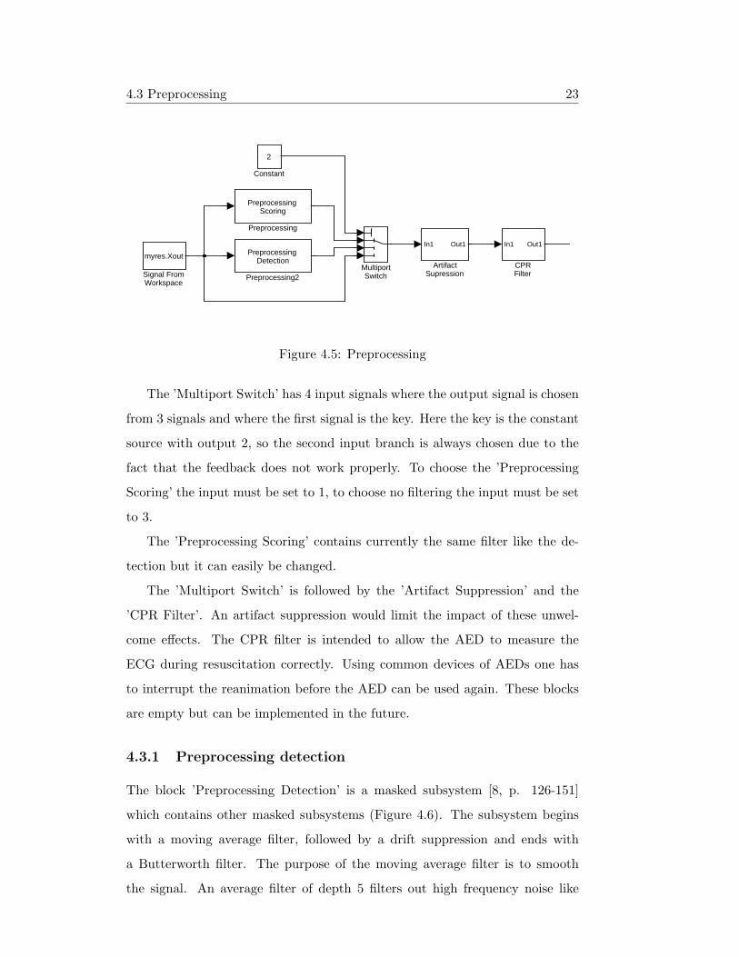
4.3 Preprocessing

After the signal is loaded from the Matlab workspace the preprocessing can

begin (Figure 4.5). The signal is split up into 3 branches where in one branch

the signal is passed unchanged and the other two branches have special filters.

A ’Multiport Switch’ chooses the desired filter-method. Right now always the

’Preprocessing Detection’ is chosen. The idea is to feedback the result of the

algorithm, whether VF is detected or not, to change the preprocessing to get a

more adequate filter-method. Unfortunately the performance of the simulation

suffers extremely when this is done. For future work it is recommended to solve

this problem.

4.3 Preprocessing 23

myres.Xout

Signal FromWorkspace

Preprocessing Detection

Preprocessing2

Preprocessing Scoring

Preprocessing

Preprocessing FFT

Pre-FFTMultiportSwitch

2

Constant

In1 Out1

CPRFilter

In1 Out1

ArtifactSupression

Figure 4.5: Preprocessing

The ’Multiport Switch’ has 4 input signals where the output signal is chosen

from 3 signals and where the first signal is the key. Here the key is the constant

source with output 2, so the second input branch is always chosen due to the

fact that the feedback does not work properly. To choose the ’Preprocessing

Scoring’ the input must be set to 1, to choose no filtering the input must be set

to 3.

The ’Preprocessing Scoring’ contains currently the same filter like the de-

tection but it can easily be changed.

The ’Multiport Switch’ is followed by the ’Artifact Suppression’ and the

’CPR Filter’. An artifact suppression would limit the impact of these unwel-

come effects. The CPR filter is intended to allow the AED to measure the

ECG during resuscitation correctly. Using common devices of AEDs one has

to interrupt the reanimation before the AED can be used again. These blocks

are empty but can be implemented in the future.

4.3.1 Preprocessing detection

The block ’Preprocessing Detection’ is a masked subsystem [8, p. 126-151]

which contains other masked subsystems (Figure 4.6). The subsystem begins

with a moving average filter, followed by a drift suppression and ends with

a Butterworth filter. The purpose of the moving average filter is to smooth

the signal. An average filter of depth 5 filters out high frequency noise like

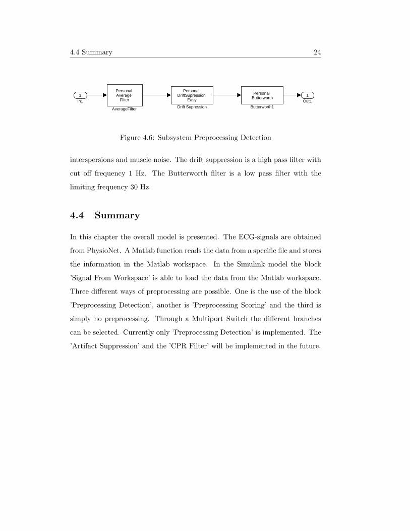
4.4 Summary 24

1Out1

Personal DriftSupression

Easy

Drift Supression

Personal Butterworth

Butterworth1

Personal Average

Filter

AverageFilter

1In1

Figure 4.6: Subsystem Preprocessing Detection

interspersions and muscle noise. The drift suppression is a high pass filter with

cut off frequency 1 Hz. The Butterworth filter is a low pass filter with the

limiting frequency 30 Hz.

4.4 Summary

In this chapter the overall model is presented. The ECG-signals are obtained

from PhysioNet. A Matlab function reads the data from a specific file and stores

the information in the Matlab workspace. In the Simulink model the block

’Signal From Workspace’ is able to load the data from the Matlab workspace.

Three different ways of preprocessing are possible. One is the use of the block

’Preprocessing Detection’, another is ’Preprocessing Scoring’ and the third is

simply no preprocessing. Through a Multiport Switch the different branches

can be selected. Currently only ’Preprocessing Detection’ is implemented. The

’Artifact Suppression’ and the ’CPR Filter’ will be implemented in the future.

Chapter 5

Fourier transform

After the preprocessing the signal is still in the time domain. But it is neces-

sary to have the signal in the frequency domain. To change the domains the

fast Fourier transform (FFT) is used. Fourier analysis is extremely useful for

data analysis, as it breaks down a signal into constituent sinusoids of different

frequencies.

5.1 Discrete Fourier transform

The signal exists in sample-based form therefore the discrete Fourier transform

(DFT) is used to perform the transform. The fast Fourier transform is an

efficient algorithm for computing the DFT of a sequence; it is not a separate

transform. Details on the Fourier transform can be found in [7], [9], [11], and

[16].

5.2 Preprocessing FFT

The block ’Preprocessing FFT’ is another masked subsystem. It contains a

block ’Buffer’. The Buffer block redistributes the input samples to a new frame

size, larger or smaller than the input frame size. Buffering to a larger frame

size, like in this case, yields an output with a slower frame rate than the input,

as illustrated in Figure 5.1.

25

5.2 Preprocessing FFT 26

Figure 5.1: General principle of buffering

Sample-based inputs are interpreted by the Buffer block as independent

channels of data. Thus, a sample-based length-N vector input is interpreted

as N independent samples. In our case the input vector has the length 1.

In sample-based operation, the Buffer block creates frame-based outputs from

sample-based inputs. A sequence of sample-based length-N vector inputs (1-D,

2-D row, or 2-D column) is buffered into an M0×N matrix, where M0 is specified

by the Output buffer size parameter. That is, each input vector becomes a row

in the N-channel frame-based output matrix. When M0 = 1, the input is simply

passed through to the output, and retains the same dimension. Sample-based

full-dimension matrix inputs are not accepted. The Buffer overlap parameter,

L, specifies the number of samples (rows) from the current output to be repeated

in the next output where L < M0. For 0 ≤ L < M0, the number of new input

samples that the block acquires before propagating the buffered data to the

output is the difference between the Output buffer size and Buffer overlap,

M0−L. The output frame period (M0−L) ∗Tsi is equal to the input sequence

sample period Tsi, when the Buffer overlap is M0 − 1. For L < 0, the block

simply discards L input samples after the buffer fills, and outputs the buffer

with period (M0−L)∗Tsi, which is longer than the zero-overlap case. Figure 5.2

shows the input dialog for the block. [21]

The Output buffer size has always the value 2048, because it is not possible

to use a variable for the parameter. With a sample-time of 0.004 seconds the

length of one frame is 8.192 seconds. This is the time interval on which the

FFT will be performed. The other parameter Buffer overlap is calculated with

the variable bufferover which comes from the masked subsystem Preprocessing

5.3 Window function 27

Figure 5.2: Buffer block dialog

FFT. There the user can specify at which rate the FFT is executed. If he or

she chooses 8.192 seconds the FFT generates an output every 8.192 seconds. If

2 seconds are selected, output is generated every 2 seconds.

To use this variable bufferover in the Buffer block this time must be divided

by the sample time to get the number of samples, which corresponds to the

time. This number must be subtracted from the original 2048 samples to get

the real Buffer overlap.

5.3 Window function

At this stage of the signal processing the data exists in frames of 2048 samples.

These frames are used to perform the FFT on them. 2048 samples accord to

8.192 seconds in time with a sample-time of 0.0004 seconds. So the FFT will

be executed on a 8.192 seconds long interval of the signal. To avoid steps at

the beginning and the end of this interval and guarantee a smooth transition

a window function is inserted before the Fourier transform. Steps can have an

distorted impact on the output.

The block ’Window function’ has several operation modes. Here the mode

5.3 Window function 28

Figure 5.3: Signal before Hamming window

Figure 5.4: Signal after use of a Hamming window

5.4 FFT block 29

Apply window to input is chosen. In this mode the block computes an M/times1

window vector (M is in this case set to 2048) w, and multiplies the vector

element-wise with each of the N channels in the M/timesN input matrix u.

(N is in this case 1) A length-M vector input is treated as an M/times1 matrix.

The output y always has the same dimension as the input. If the input is frame-

based, the output is frame-based; otherwise, the output is sample-based.

As Window Type Hamming is chosen which has good characteristics for

the further signal processing. The leakage-factor is very small and the spectral

resolution is high. Not at least because there is a big number of samples - the

window length is very long. So the error caused by the Window function is very

small. Figure 5.3 and Figure 5.4 illustrate how the Window function works in

the time domain. More information about window functions can be found in

[7] and [10].

5.4 FFT block

The FFT block computes the fast Fourier transform (FFT) of each channel in

the M/timesN or length-M input where M must be a power of two. That is

the reason why 2048 samples per frame are chosen in the section Preprocessing

FFT. The output is always a complex-valued vector.

The input dialog of the ’FFT’ block offers two parameters (Figure 5.5).

One is the Twiddle factor computation parameter, which determines how the

block computes the necessary sine and cosine terms. When Table lookup is

selected the block computes and stores the trigonometric values before the

simulation starts, and retrieves them during the simulation. If Trigonometric

fcn is chosen, the block computes sine and cosine values during the simulation.

The effect of Table lookup is that the block usually runs much more quickly, but

requires extra memory for storing the precomputed trigonometric values. Vice

versa Trigonometric fcn results in a slower simulation but does not need extra

memory. Due to the real-valued input and the output ordering, which is linear,

a Radix-2 decimation-in-time (DIT) algorithm is used by Matlab to compute

the FFT.

5.5 Postprocessing 30

Figure 5.5: Input dialog for ’FFT’ block

5.5 Postprocessing

There are three more blocks required to work on the output of the ’FFT’ block.

The output is complex-valued and to convert it to real numbers the ’Abs’ block

is used which delivers the absolute value of the input. Next follows a ’Gain’

block with the factor 2, because only half of the FFT values (except the first

value with frequency 0) in the spectrum are computed. Here all elements are

multiplied with the factor 2 because during the preprocessing the high pass

filtered out the very low frequencies. So the error which arises can be neglected.

Finally a conversion of the sample-based data into frame-based data is needed.

The ’Frame Status Conversion’ block passes the input through to the output

and sets the output frame status to the Output signal parameter, which can be

either frame-based or sample-based. Here frame-based is selected which leads

to the desired result.

5.6 Summary 31

5.6 Summary

To change the signal from the time-domain into the frequency-domain the fast

Fourier transform is used. The FFT is a special form of the discrete Fourier

transform with a high performance. To generate frame-based data, which are

necessary for the FFT block, preprocessing is done. A Hamming window func-

tion is applied to the signal. The FFT block generates a complex-valued sample-

based output from which absolute values are computed and then transformed

to frame-based by the postprocessing.

Chapter 6

Barros algorithm

As written in Section 1.6 this algorithm was invented in 1989 by Barro and

others [5]. To implement it two more blocks are necessary after the prepro-

cessing and the Fourier transform. First a filter block ’Barro Threshold Filter’

is needed which filters out all values of the spectrum (stored in a frame) that

lie under a threshold of 5% of the maximum value. For frames 2048 values

are used. Afterwards the algorithm is computed in the block ’BarroAlgorithm

Parameter Computation’. Both blocks are implemented as S-Functions.

6.1 S-Functions

An S-Function is a computer language description of a Simulink block. S-

Functions can be written in Matlab, C, C++, Ada, or Fortran. C, C++, Ada,

and Fortran S-Functions are compiled as MEX-files using the mex utility. As

with other MEX-files, they are dynamically linked into Matlab when needed.

The form of an S-Function is very general and can accommodate continuous,

discrete, and hybrid systems. S-Functions allow someone to add his or her own

blocks to Simulink models.

After the S-Function is written, its name can be placed in an S-Function

block (available in the Functions and Tables block library). The user interface

can additionally be customized by masking. For details on writing S-Functions

see [8] and [20].

32

6.2 Using S-Functions in models 33

Figure 6.1: S-Function overview

6.2 Using S-Functions in models

To incorporate an S-Function into a Simulink model, drag an S-Function block

from Simulink Functions and Tables block library into the model. Then specify

the name of the S-Function in the S-Function name field of the S-Function

blocks dialog box, as illustrated in the following figure.

In this example (Figure 6.1), the model contains two instances of an S-

Function block. Both blocks reference the same source file (mysfun, which can

be either a C MEX-file or an M-file). If both a C MEX-file and an M-file

have the same name, the C MEX-file takes precedence and is the file that the

S-Function uses.

6.3 Threshold filter

This block is implemented as a masked subsystem with underlying S-Function.

It follows the specification by Barro [5] that the values in the signal, which lie

under a certain threshold, must be filtered out and set to zero. The threshold

6.4 Parameter computation 34

is calculated by finding the maximum in the considered frame and multiplying

it by 0.05 which is 5%. This percentage value can be modified in the block

by the user. Regular values reach from 0 to 1. The used S-Function is called

’BarroThresholdFilter’ and is written in C. The input must be a frame, the

output is then a frame too. All S-Functions are implemented in C, because

only C S-Functions provide the ability to use frame-based data. Information

about C can be obtained from [14] and [18].

6.4 Parameter computation

The block ’BarroAlgorithm Parameter Computation’ is also a masked subsys-

tem with underlying S-Function. There is no parameter that can be chosen.

The purpose of this block is to decide, whether or not ventricular fibrillation

occurs. The specification of the algorithm are taken from [5]. The following

parameters are calculated:

First spectral moment normalized (FSMN) which is the center of gravity

of the spectrum. The algorithm figures out the maximum amplitude in the

considered sequence and the corresponding frequency, which is the reference

frequency. Then the following expression is calculated:

FSMN =1F

m2∑j=m1

|a(ωj)| ∗ ωj

m2∑j=m1

|a(ωj)|

F is the reference frequency, ωj is the frequency at a given index and a(ωj)

the corresponding complex FFT-amplitude. The sums are calculated from 0.5 -

100 Hz. The value of the FSMN will depend on the distribution of the signal over

the entire spectrum. A high concentration around the reference frequency will

result in small numbers whereas a wide distribution towards higher frequencies

will cause larger numbers. Ventricular fibrillation is characterized by a narrow

band around the reference frequency and the normal sinus rhythm is associated

by a larger dispersion of the area towards higher harmonics.

6.5 Summary 35

Next follows the parameter A1, which is the ratio of the area of two different

frequency bands. In the numerator the band reaches from 0.5 Hz to F2 where F

is the reference frequency. The denominator consists of the band from 0.5 Hz to

20F. This is a descriptor crucial in distinguishing between ventricular fibrillation

and imitative artifacts. In general, high values of A1 are indicative of artifacts.

A2 is the ratio of the area contained in the range 0.7F to 1.4F and the total

area considered (0.5 Hz - 20F). The parameter provides information about the

relative distribution of area around the reference frequency. It is high in the

ventricular fibrillation category.

Finally A3 is the ratio of the area contained around the second to eight

harmonic and the total area considered. To estimate the value for each harmonic

the area contained in a band of 0.6F in width, centered on the harmonic. This

descriptor is related to the repetition of peaks at frequencies which are multiples

of the reference frequency. The parameters value is high in the case of records

with dominant sinus rhythm and is very low in the case of VF and imitative

artifacts.

These parameters are used to determine if the signal is VF or SR. VF is

detected if FSMN ≤ 1.55 && A1 ≤ 0.19 && A2 ≥ 0.45 && A3 ≤ 0.09.

This decision is the first output of the block, where 1 means VF and 0

means SR. The outputs 2 to 5 are A1, A2, A3 and FSMN. These outputs can

be watched easily with a scope. This enables analysis and optimization for the

user.

6.5 Summary

S-Functions are used to include self-written blocks into Simulink. This can be

done in MATLAB, C, C++, Ada, or Fortran. The algorithm of Barro is split

up in two blocks. One filters out the values which lie under a threshold and the

other is responsible for the computation of various parameters. Both blocks are

implemented as S-Functions in C.

Chapter 7

Spectral algorithm

The purpose of this chapter is to provide more parameters for the analysis of

the spectrum. It would be very useful to get a better performance than with

Barros algorithm. The ’Spectrum Scope’ and the block ’Get Annotated Data’

are described too.

7.1 Parameter computation

’Spectral Algorithm’ is the name of a block which delivers eight parameters

based on the ideas of Amann and Unterkofler. The input signal is the output

from the block ’Barro Threshold Filter’ (reuse of a block from Barros algo-

rithm) which is frame-based. Two parameters (Frequency 1 and Frequency

2) determine the frequency-band which will be considered for the first three

parameters calculated. Four more parameters can be selected which limit the

frequency-range for the computation of the other five parameters. In Figure 7.1

for example 4.33Hz and 20Hz are chosen as Frequency 1 and 2, and 0.3Hz, 3.5Hz,

9Hz and 50Hz are set as limits.

7.1.1 Parameters 1 to 3

The block computes three parameters within Frequency 1 and 2 :

• The first is the dominant frequency, which is the frequency in the con-

sidered frequency-band with the highest amplitude. A relatively high

36

7.1 Parameter computation 37

Figure 7.1: Input dialog for ’Spectral Algorithm’

dominant frequency signalizes VF whereas a lower dominant frequency

indicates SR.

• Next is the mean frequency which is given by the expression

Fmean =

m2∑j=m1

|a(ωj)| ∗ ωj

m2∑j=m1

|a(ωj)|

where m1 is the lower and m2 the higher frequency-index. a(ωj) is the

complex FFT-amplitude at a given index j and ωj the corresponding

frequency. The idea is to obtain the mean frequency in the considered

frequency-band which helps to distinguish between SR and VF. During

SR the mean frequency is higher then during VF. Figure 7.2 confirms that

statement. After 220 seconds the SR changes to VF which results in an

abrupt decline of the mean frequency.

7.1 Parameter computation 38

• The amplitude mean spectral area (AMSA) is calculated by

AMSA =m2∑

j=m1

|a(ωj)| ∗ (ωj − ωj−1)

where m1 is the lower and m2 the higher frequency-index. a(ωj) is the

complex FFT-amplitude at a given index j and ωj the corresponding

frequency. All differences (ωj − ωj−1) have the same length.

7.1.2 Parameters 4 to 8

The second set of parameters (five) which are calculated correlate to the

frequency-limits 1 to 4. The limits are n1, n2, n3, and n4. Then the parameters

are:

• E100 is the spectral energy over the whole considered frequency-range

from n1 to n4.

E100 =n4∑

j=n1

|a(ωj)|2

• E1 is the spectral energy from n1 to n2 normalized by E100.

E1 =

n2∑j=n1

|a(ωj)|2

E100

• E2 is the spectral energy from n2 to n3 normalized by E100.

E2 =

n3∑j=n2

|a(ωj)|2

E100

• E3 is the spectral energy from n3 to n4 normalized by E100.

E3 =

n4∑j=n3

|a(ωj)|2

E100

The idea is to distinguish between SR and VF by looking at the spe-

cific frequency-bands. SR contains energy in the very low and the high

frequency-areas, wheras VF has its maximum in the middle frequency-

area. If E1 + E3 is high and E2 is low, SR is expected and if E1 + E3 is

low and E2 is high, VF is expected.

7.1 Parameter computation 39

4

4.5

5

5.5

6

6.5

7

7.5

8

8.5

9Dominant Frequency

5

5.5

6

6.5

7

7.5

8

8.5

9

9.5

10Mean Frequency

0 50 100 150 200 250 300 350 400 450 500100

200

300

400

500

600

700

800AMSA

Time offset: 0

Figure 7.2: Parameters dominant frequency, mean frequency, and AMSA dis-

played by scope

7.2 Spectral decision 40

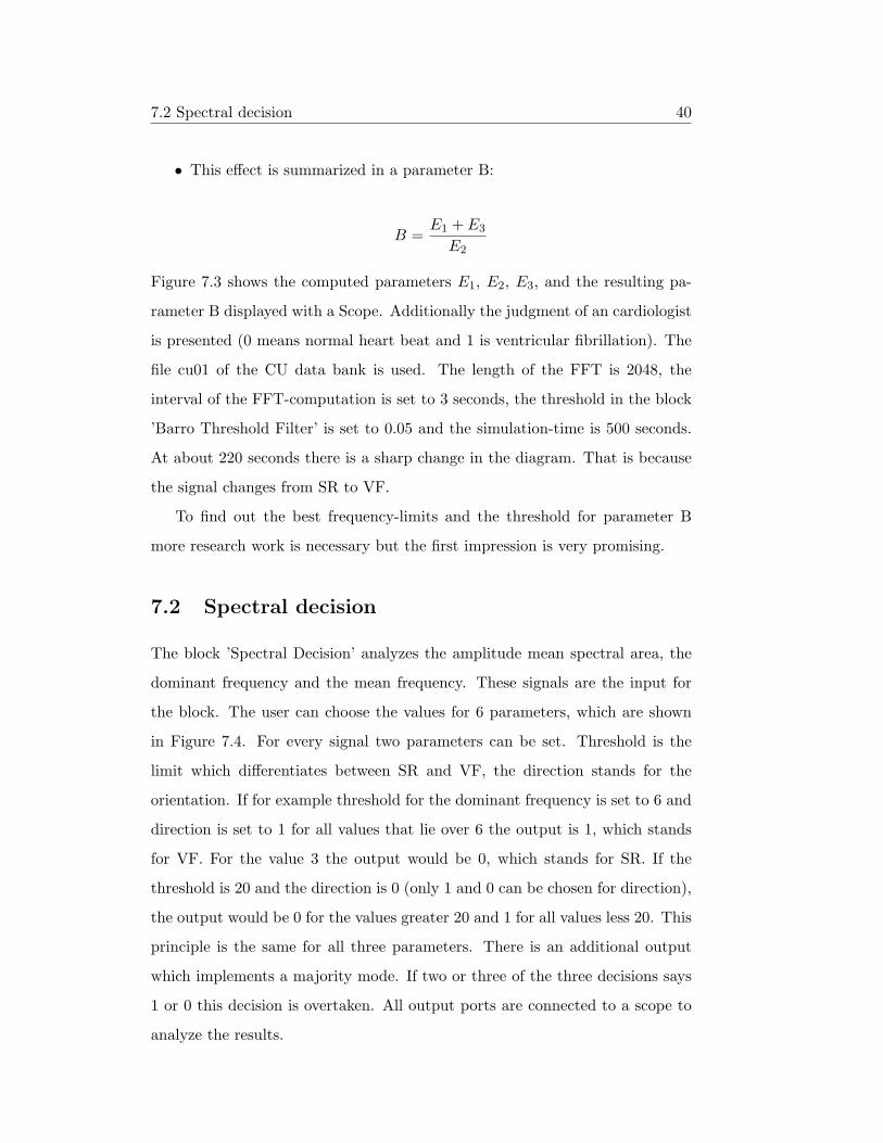
• This effect is summarized in a parameter B:

B =E1 + E3

E2

Figure 7.3 shows the computed parameters E1, E2, E3, and the resulting pa-

rameter B displayed with a Scope. Additionally the judgment of an cardiologist

is presented (0 means normal heart beat and 1 is ventricular fibrillation). The

file cu01 of the CU data bank is used. The length of the FFT is 2048, the

interval of the FFT-computation is set to 3 seconds, the threshold in the block

’Barro Threshold Filter’ is set to 0.05 and the simulation-time is 500 seconds.

At about 220 seconds there is a sharp change in the diagram. That is because

the signal changes from SR to VF.

To find out the best frequency-limits and the threshold for parameter B

more research work is necessary but the first impression is very promising.

7.2 Spectral decision

The block ’Spectral Decision’ analyzes the amplitude mean spectral area, the

dominant frequency and the mean frequency. These signals are the input for

the block. The user can choose the values for 6 parameters, which are shown

in Figure 7.4. For every signal two parameters can be set. Threshold is the

limit which differentiates between SR and VF, the direction stands for the

orientation. If for example threshold for the dominant frequency is set to 6 and

direction is set to 1 for all values that lie over 6 the output is 1, which stands

for VF. For the value 3 the output would be 0, which stands for SR. If the

threshold is 20 and the direction is 0 (only 1 and 0 can be chosen for direction),

the output would be 0 for the values greater 20 and 1 for all values less 20. This

principle is the same for all three parameters. There is an additional output

which implements a majority mode. If two or three of the three decisions says

1 or 0 this decision is overtaken. All output ports are connected to a scope to

analyze the results.

7.2 Spectral decision 41

0

0.1

0.2

0.3

0.4E1

0

0.2

0.4

0.6

0.8

1E2

0

0.1

0.2

0.3

0.4E3

0

0.5

1

1.5B

0 50 100 150 200 250 300 350 400 450 500-0.5

0

0.5

1

1.5Cardiologist

Time offset: 0

Figure 7.3: Parameters E1, E2, E3, B, and classification of cardiologist displayed

by scope

7.3 Spectrum scope 42

Figure 7.4: Input dialog for ’Spectral Decision’

7.3 Spectrum scope

It is very useful to see the spectrum of the signal over the whole time. This

is done by the subsystem ’Spectrum Scope’. The difference between a masked

subsystem and a normal subsystem is, that a subsystem can be changed by the

user in the model. This feature is needed here. Figure 7.5 illustrates how the

spectrum scope works.

The input signal comes from the end of the Fourier part before the Barro

threshold filter. The signal is frame-based and one frame consists of N samples

(In Figure 7.5 there are 2048 samples per frame). The whole frame includes

the frequency spectrum in an interval ofN

FSseconds, where FS is the sampling-

frequency. The frequency spectrum ranges from 0 to FS . But there is no new

information betweenFS

2and FS because the spectrum is symmetric around

FS

2. For a visual presentation only the first

N

2samples can be considered.

But due to the fact that the amplitudes beyond 35 Hz are very small only the

7.3 Spectrum scope 43

uT

Transpose

Submatrix

MatrixViewer

MatrixViewer

ToSample

Frame StatusConversion1

1In1

[300x166]

[2048x1] [300x1][300x1] [166

[16

Figure 7.5: Subsystem ’Spectrum Scope’

firstN ∗ 35 Hz

FSsamples are used. When FS is 250 Hz and the frame has 2048

samples the first2048 ∗ 35 Hz

250 Hz= 286.72 samples would be considered.

This selection happens with the block ’Submatrix’. In Figure 7.5 the frame-size

changes from 2048 x 1 to 300 x 1 . Next follows a conversion to a sample-based

and vector-sized signal by the block ’Frame Status Conversion’. This is the first

step in buffering the spectrum over time. Then the block ’Buffer’ is applied to

the signal. By setting the parameter Output buffer size to Bs and Buffer overlap

to Bo the whole spectrum is generated at the end of the simulation. Because the

input is sample-based and vector-sized each vector is considered as a channel.

The generated output will be frame-based in the dimension of Bs x 300. Bs

has to be chosen in dependence of the simulation time and the parameters of

the FFT block.

For example: Let the simulation-time Ts be 500 seconds and the calculation-

interval of the Fourier transform FFTinterval 3 seconds. The number of neces-

sary frames (represented by Output buffer size Bs) is calculated by the expres-

sion:

Bo =Ts

FFTinterval=

500 s

3 s= 166.67

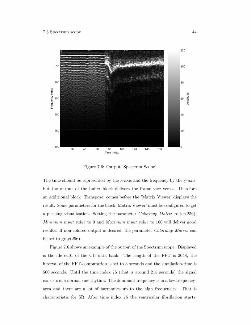
7.3 Spectrum scope 44

20 40 60 80 100 120 140 160

50

100

150

200

250

300

Time Index

Freq

uenc

y In

dex

0

20

40

60

80

100

120

Am

plitu

de

Figure 7.6: Output ’Spectrum Scope’

The time should be represented by the x-axis and the frequency by the y-axis,

but the output of the buffer block delivers the frame vice versa. Therefore

an additional block ’Transpose’ comes before the ’Matrix Viewer’ displays the

result. Some parameters for the block ’Matrix Viewer’ must be configured to get

a pleasing visualization. Setting the parameter Colormap Matrix to jet(256),

Minimum input value to 0 and Maximum input value to 160 will deliver good

results. If non-colored output is desired, the parameter Colormap Matrix can

be set to gray(256).

Figure 7.6 shows an example of the output of the Spectrum scope. Displayed

is the file cu01 of the CU data bank. The length of the FFT is 2048, the

interval of the FFT-computation is set to 3 seconds and the simulation-time is

500 seconds. Until the time index 75 (that is around 215 seconds) the signal

consists of a normal sine rhythm. The dominant frequency is in a low frequency-

area and there are a lot of harmonics up to the high frequencies. That is

characteristic for SR. After time index 75 the ventricular fibrillation starts.

7.4 Annotated data 45

1Out1

In1

In2

In3

Out1

TriggeredSubsystem1

PulseGenerator

ToFrame

Frame StatusConversion2

ToFrame

Frame StatusConversion1

myres.annot

Constant1

myres.atrtime

Constant

Clock

[204x1]

[204x1]

[204x1]

[204x1][204x1]

[204x1]

Figure 7.7: Subsystem ’Get Annotated Data’

Here is a strong concentration of the amplitudes in the spectrum around the

dominant frequency, which lies higher then in case of SR. The harmonics are

much weaker in the case of VF.

7.4 Annotated data

The various algorithms deliver decisions whether VF or SR has occured. To

compare the validity of these decisions with the diagnosis of a cardiologist extra

information is needed which is stored in the structure myres in the Matlab-

workspace.

The block ’Get Annotated Data’ is a masked subsystem which is displayed

in Figure 7.7. The access uses two normal ’Constant’ blocks. One block reads

the time and the other the data. The two blocks have sample-based 1D-vector

output that varies in size from signal to signal. The length of these two vari-

ables is not prescribed but they must be equal. (In Figure 7.7 for example the

dimension is 204.) For every (time)sample in the variable myres.atrtime exists

a (data)sample in myres.annot. There are more then 40 different codes for the

signal, but only two are considered. Value 32 in myres.annot means start of VF

and value 33 means end of VF. If for example the 73rd value in myres.annot is

a value 32 the according time would be the 73rd value in myres.atrtime.

Both outputs of the ’Constant’ blocks are changed from sample-based into

7.5 Summary 46

frame-based by two ’Frame Status Conversion’ blocks. That is done because it

makes the processing through a S-Function possible. The S-Function annotData

is part of a triggered subsystem. It is triggered with a ’Pulse Generator’ that

creates a rectangular signal with a period of 2 seconds. The triggered subsystem

reacts on every change, what happens every second. That means, that the S-

Functions reads the input every second and generates the output also every

second. The S-Function has 3 inputs. Two inputs from the structure myres

and the simulation time of the block ’Clock’.

The algorithm for the output in the S-Function distinguishes between two

values: 1 means VF and 0 means no VF. The output is updated every second,

due to the trigger-signal. This signal can now be connected with a scope to

compare it with the results of the algorithm.

7.5 Summary

The spectrum is analyzed by the ’Spectrum Algorithm’ and some character-

istic parameters are obtained. The user can specify some frequency-limits for

the computation of these parameters. An additional block ’Spectral Decision’

compares the parameters for a final decision. This final decision is compared

with the diagnosis of a cardiologist which comes from the block ’Get Annotated

Data’. The ’Spectrum scope’ provides a useful visualization of the spectrum

during the whole simulation-time.

Chapter 8

Discussion

8.1 Conclusion

There is still need for an improvement of the algorithms that analyze ECG-

signals in AEDs. Until now these algorithms were implemented in Matlab at

the FH-Vorarlberg. This implementations are not very user-friendly and it is

not easy to make changes of the code. The solution presented in this diploma

thesis is built with the tool Simulink which is an extension of Matlab.

The great benefits of the created simulation environment in Simulink is

the clear way the simulation works, the ability of changing parameters and

algorithms easily and the various possibilities to visualize the signals. It is also

a big advantage that people, who are not familar with Simulink, can learn the

necessary knowledge very fast.

The realized model consists of several S-Functions. The advantage is the

high performance and the ability of creating personal blocks. They are all

written in C and compiled with the Matlab-compiler MEX. There is also a

variety of masked subsystems because of the high user-friendliness and the

possibility of reuse in other models.

This diploma thesis only deals with the creation of the simulation environ-

ment of the spectral algorithms.

47

8.2 Outlook 48

8.2 Outlook

Now the optimization of the implemented algorithms can start by the relevant

persons. That means the optimization of various parameters and thresholds.

But there is still some work to do on the model.

In the preprocessing-part the block ’Preprocessing Scoring’ needs to be

changed because it consists of the same filter like ’Preprocessing Detection’.

The feedback from the decision if VF or SR occurs leads to a very bad per-

formance, so it is not implemented yet. This problem should be solved in the

future.

The blocks ’Artifact Suppression’ and ’CPR Filter’ are empty and need to

be implemented. That was also a reason for implementing algorithms that work

in the frequency-domain because of the potential for further extensions.

It is planed to implement other algorithms like the TCI-algorithm (threshold

crossing intervals) or the ACF-algorithm (autocorrelation) in the future. The

gained experience and knowledge of this diploma thesis can build a foundation

for that work.

Bibliography

[1] A. Amann, R. Tratnig, and K. Unterkofler, Reliability of fibrillation detec-

tion algorithms in automatic external defibrillators (AEDs), Department

of Computer Science, FH-Vorarlberg, preprint 2004.

[2] American Heart Association, Heart Disease and Stroke Statistics - 2004

Update, Dallas, Tex.: American Heart Association 2003.

[3] American Heart Association, Heart and Stroke Facts, Dallas, Tex.: Amer-

ican Heart Association 2003.

[4] A. Angermann, M. Beuschel, M. Rau und U. Wohlfarth, Matlab - Simulink

- Stateflow. Grundlagen, Toolboxen, Beispiele, 2. Aufl. Oldenbourg 2002.

[5] S. Barro, R. Ruiz, D. Cabello, and J. Mira, Algorithmic sequential decision-

making in the frequency domain for life threatening ventricular arrhythmias

and imitative artefacts: a diagnostic system, J. Biomed. Eng. 11, 320-328

(1989).

[6] O. Beucher, Matlab und Simulink. Grundlegende Einfuhrung, 2. Aufl.

Addison-Wesley, Pearson Studium, Munchen 2002.

[7] T. Butz, Fouriertransformation fur Fussganger, 3. Aufl. Teubner, Wies-

baden 2003.

[8] J. B. Dabney and T. L. Harman, Mastering Simulink, Pearson Prentice

Hall, N.J. 2004.

[9] P. Gerdsen und P. Kroger, Digitale Signalverarbeitung in der Nachrichten-

ubertragung, 2. Aufl. Springer, Berlin 1996.

49

BIBLIOGRAPHY 50

[10] D. Ch. von Grunigen, Digitale Signalverarbeitung, 2. Aufl. Fachbuchverlag

Leipzig 2002.

[11] E. Herter und W. Lorcher, Nachrichtentechnik. Ubertragung - Vermittlung

- Verarbeitung, 7. Aufl. Hanser, Munchen 1994.

[12] J. Hoffmann, Matlab und Simulink in Signalverarbeitung und Kommu-

nikationstechnik. Beispielorientierte Einfuhrung. Simulation praxisnaher

Prozesse und Systeme, Addison-Wesley, Munchen 1999.

[13] I. Jekova, Comparison of five algorithms for the detection of ventricular

fibrillation from the surface ECG, Physiol. Meas. 21, 429-439 (2000).

[14] U. Kaiser, C/C++. Von den Grundlagen zur professionellen Program-

mierung, Galileo Press, Bonn 2000.

[15] R. Liddle, C. S. Davies, M. Colquhoun, and A. J. Handley, ABC of Re-

suscitation. The automated external defibrillator, BMJ (Brithish Medical

Journal) 327, 1216-1218 (2003).

[16] S. D. Stearns und D. R. Hush, Digitale Verarbeitung analoger Signale,

7. Aufl. Oldenbourg 1999.

[17] T. D. Valenzuela, D. J. Roe, G. Nichol, L. L. Clark, D. W. Spaite, and

R. G. Hardman, Outcomes of rapid defibrillation by security officers after

cardiac arrest in casinos, New England Journal of Medicine 343, 1206-1209

(2000).

[18] K. Zeiner, Programmieren lernen mit C, Hanser, Munchen 1994.

[19] The MathWorks, Simulink. Model-Based and System-Based Design. Using

Simulink, Sixth printing, The MathWorks, Inc., Natick, MA 2003.

[20] The MathWorks, Simulink. Model-Based and System-Based Design. Writ-

ing S-Functions, Third printing, The MathWorks, Inc., Natick, MA 2002.

[21] The MathWorks, Inc., http://www.mathworks.com

BIBLIOGRAPHY 51

[22] Physionet: http://www.physionet.org

[23] Physionet: http://www.physionet.org; Examples:

http://www.physionet.org/physiobank/database/mitdb

[24] Physionet: http://www.physionet.org; Examples:

http://www.physionet.org/physiobank/database/cudb