Create Workbooks Using Microsoft Excel 2010 - Jones & Bartlett

Create Workbooks Using Microsoft Excel 2010

Chapter ObjectivesAft er completing this chapter, you will be able to do the following:

• Identify Microsoft Excel 2010 components.• Enter and modify data in a worksheet.• Navigate within a worksheet.• Copy, cut, paste, and move cells.• Modify column and row settings.• Calculate totals.• Apply formatting to cells.• Display formulas.• Save and print a workbook.

Microsoft Excel 2010 is a spreadsheet application used to organize,

manipulate, and chart data. Microsoft Excel 2010 can be used to

track income and expenses, perform mathematical calculations,

and analyze data to make informed decisions.

In this chapter, you will become acquainted with various

components of Microsoft Excel 2010. You will create a workbook,

modify column and row settings, and calculate totals. Additionally,

you will format the workbook to give it a professional appearance.

66666666666666666666666666666666666666666666666666666666666666679446_CH06_321-372.indd Page 321 06/12/12 8:35 PM user-f39979446_CH06_321-372.indd Page 321 06/12/12 8:35 PM user-f399 F-399F-399

© Jones & Bartlett Learning, LLC. NOT FOR SALE OR DISTRIBUTION

Identify Microsoft Excel 2010 ComponentsYou will open Microsoft Excel 2010 and get acquainted with its components.

Hands-On Exercise: Launch Microsoft Excel 2010

① Click the Start button.

② Click All Programs .

③ Click Microsoft Offi ce . You may need to scroll through the Start menu to locate the folder.

④ Click Microsoft Excel 2010 .

⑤ A new blank workbook displays (Figure 6.1).

Figure 6.1 Microsoft Excel 2010 Workbook

Quick Access ToolbarRibbon Dialog box launcher

Scroll bar

Zoom controlsView buttons

Table 6.1 illustrates many common elements and key terms used in Microsoft Offi ce 2010 applications.

322 Chapter 6 Create Workbooks Using Microsoft Excel 2010



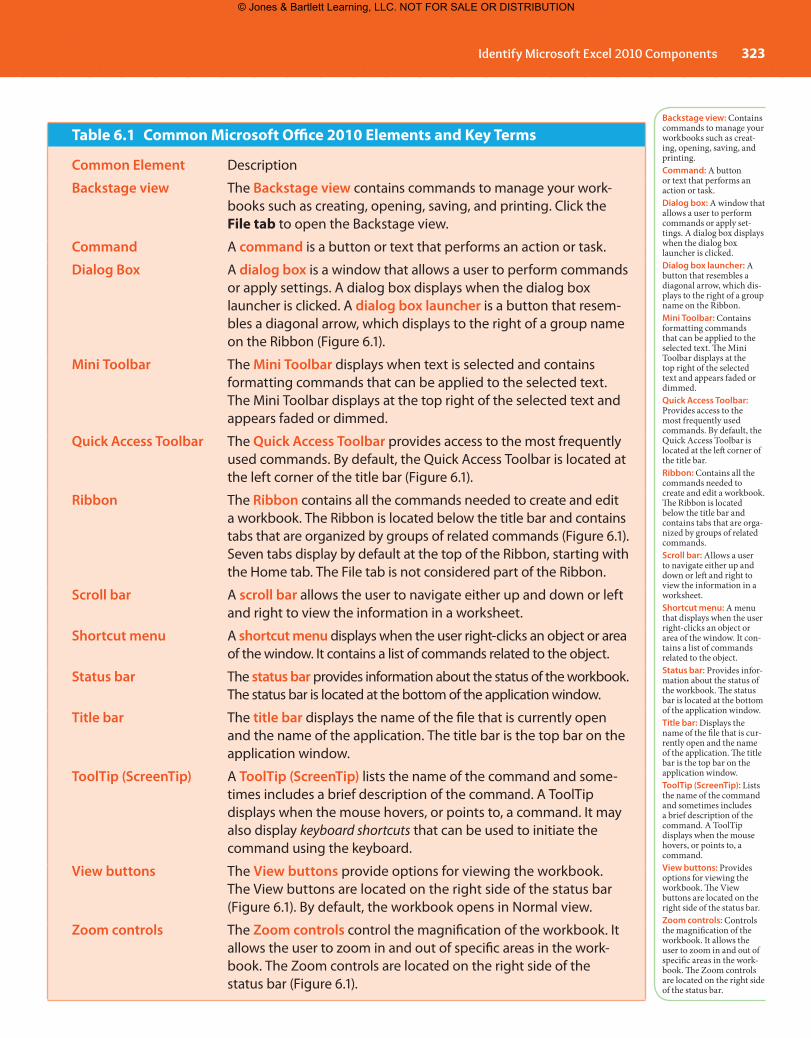
Table 6.1 Common Microsoft Offi ce 2010 Elements and Key Terms

Common Element Description

Backstage view The Backstage view contains commands to manage your work-books such as creating, opening, saving, and printing. Click the File tab to open the Backstage view.

Command A command is a button or text that performs an action or task.

Dialog Box A dialog box is a window that allows a user to perform commands or apply settings. A dialog box displays when the dialog box launcher is clicked. A dialog box launcher is a button that resem-bles a diagonal arrow, which displays to the right of a group name on the Ribbon (Figure 6.1).

Mini Toolbar The Mini Toolbar displays when text is selected and contains formatting commands that can be applied to the selected text. The Mini Toolbar displays at the top right of the selected text and appears faded or dimmed.

Quick Access Toolbar The Quick Access Toolbar provides access to the most frequently used commands. By default, the Quick Access Toolbar is located at the left corner of the title bar (Figure 6.1).

Ribbon The Ribbon contains all the commands needed to create and edit a workbook. The Ribbon is located below the title bar and contains tabs that are organized by groups of related commands (Figure 6.1). Seven tabs display by default at the top of the Ribbon, starting with the Home tab. The File tab is not considered part of the Ribbon.

Scroll bar A scroll bar allows the user to navigate either up and down or left and right to view the information in a worksheet.

Shortcut menu A shortcut menu displays when the user right-clicks an object or area of the window. It contains a list of commands related to the object.

Status bar The status bar provides information about the status of the workbook. The status bar is located at the bottom of the application window.

Title bar The title bar displays the name of the fi le that is currently open and the name of the application. The title bar is the top bar on the application window.

ToolTip (ScreenTip) A ToolTip (ScreenTip) lists the name of the command and some-times includes a brief description of the command. A ToolTip displays when the mouse hovers, or points to, a command. It may also display keyboard shortcuts that can be used to initiate the command using the keyboard.

View buttons The View buttons provide options for viewing the workbook. The View buttons are located on the right side of the status bar (Figure 6.1). By default, the workbook opens in Normal view.

Zoom controls The Zoom controls control the magnifi cation of the workbook. It allows the user to zoom in and out of specifi c areas in the work-book. The Zoom controls are located on the right side of the status bar (Figure 6.1).

Backstage view: Contains commands to manage your workbooks such as creat-ing, opening, saving, and printing.Command: A button or text that performs an action or task.Dialog box: A window that allows a user to perform commands or apply set-tings. A dialog box displays when the dialog box launcher is clicked.Dialog box launcher: A button that resembles a diagonal arrow, which dis-plays to the right of a group name on the Ribbon.Mini Toolbar: Contains formatting commands that can be applied to the selected text. Th e Mini Toolbar displays at the top right of the selected text and appears faded or dimmed.Quick Access Toolbar: Provides access to the most frequently used commands. By default, the Quick Access Toolbar is located at the left corner of the title bar.Ribbon: Contains all the commands needed to create and edit a workbook. Th e Ribbon is located below the title bar and contains tabs that are orga-nized by groups of related commands.Scroll bar: Allows a user to navigate either up and down or left and right to view the information in a worksheet.Shortcut menu: A menu that displays when the user right-clicks an object or area of the window. It con-tains a list of commands related to the object.Status bar: Provides infor-mation about the status of the workbook. Th e status bar is located at the bottom of the application window.Title bar: Displays the name of the fi le that is cur-rently open and the name of the application. Th e title bar is the top bar on the application window.ToolTip (ScreenTip): Lists the name of the command and sometimes includes a brief description of the command. A ToolTip displays when the mouse hovers, or points to, a command.View buttons: Provides options for viewing the workbook. Th e View buttons are located on the right side of the status bar.Zoom controls: Controls the magnifi cation of the workbook. It allows the user to zoom in and out of specifi c areas in the work-book. Th e Zoom controls are located on the right side of the status bar.

Identify Microsoft Excel 2010 Components 323

79446_CH06_321-372.indd 23 06/12/12 8:35 PM user-f39979446_CH06_321-372.indd Page 323 06/12/12 8:35 PM user-f399 F-399F-399


When you open Microsoft Excel 2010, an empty workbook displays. A workbook contains a collection of worksheets, or sheets, used to organize information. A worksheet contains rows and columns that resembles a ledger. Although workbooks and spreadsheets are some-times used interchangeably, a spreadsheet is actually the type of soft ware program used to create a Microsoft Excel 2010 workbook. A workbook is similar to a notebook that has many pages. Each page in a workbook is called a worksheet, or sheet. Th ree sheets are shown by default in a workbook (Figure 6.2). Additional sheets can be inserted into a workbook and sheets can be deleted.

Th e Formula Bar is the horizontal bar located below the Ribbon (Figure 6.2). Below the Formula Bar are the column headings. Th e column headings identify the columns in the worksheet (Figure 6.2). Th e column headings contain the alphabet. Th e fi rst column is column A, the second column is B, the third column is C, continuing through column Z. Aft er column Z, the column headings are labeled with two letters of the alphabet, starting with AA, AB, and so on. Aft er column ZZ, the column headings are labeled with three letters of the alphabet, starting with AAA. Th e last column is XFD. Th e row headings identify the rows in the work-sheet (Figure 6.2). Th e row headings are numbered sequentially and start with row 1. Th ere are a maximum of 1,048,576 rows on a worksheet.

Th e intersection of a row and column is called a cell. Notice below column A, the cell has a black border around it (Figure 6.3). Th is is called the active cell. When you enter data in the worksheet, the data is placed in the active cell. You can insert text, numbers, or formulas

Formula Bar

Row headings

Column headings

Sheets

Figure 6.2 Microsoft Excel 2010 Components

Workbook: Contains a collection of work-sheets used to organize information.Worksheet: A page in a workbook.Sheet: A page in a workbook.Formula Bar: A hori-zontal bar located below the Ribbon. It displays the contents of the active cell.Column headings: Identify the columns in the worksheet.Row headings: Identify the rows in the work-sheet. Th e row headings are numbered sequen-tially and start with row 1.Cell: Th e intersection of a row and column.Active cell: Th e cell that has a black border around it. When you enter data in the work-sheet, the data is placed in the active cell.




into a cell. If you navigate to another cell, that cell becomes the active cell. You can tell which column and row contains the active cell because the column and row headings display with a gold background (Figure 6.3).

Each cell has a cell address, which is also called a cell reference. Th e cell address indicates the location of the cell in the worksheet. It is the column letter followed by the row number of the cell. When referencing the cell address, you can use either uppercase or lowercase letters to identify the column. Th e name of the active cell in Figure 6.3 is A1 or a1.

Th e cell address of the active cell displays in the Name Box on the Formula Bar (Figure 6.3). To navigate to a cell in the worksheet, type the cell address in the Name Box and press Enter. Th e cell address in the Name Box becomes the active cell.

Navigation TechniquesYou can use the mouse or keyboard to navigate within the worksheet. Clicking in a cell will make it the active cell. Press Enter to move down to the next row in the current column. Press Tab to move to the right of the active cell.

When you navigate a worksheet using the mouse, the mouse pointer may change shape and size, depending on your position within the workbook. When you move around in the cells of a worksheet, the mouse pointer displays as a block plus sign. Th e mouse pointer displays as an arrow when pointing to the commands on the Ribbon. Table 6.2 displays various ways to navigate within a worksheet.

Figure 6.3 Active Cell

Name Box

Active cell

Row and column heading of the active cell displays with gold background

Cell address (cell reference): Indicates the location of the cell in the worksheet. Th e cell address is the column letter followed by the row number of the cell.

Cell reference (cell address): Indicates the location of the cell in the worksheet. Th e cell reference is the column letter followed by the row number of the cell.

Name Box: Th e area on the Formula Bar that contains the cell address of the active cell.

Navigation Techniques 325



Table 6.2 Navigation Techniques

Key Navigation

Home Navigates to column A of the current row.

Ctrl � Home Navigates to the beginning of the worksheet.

Ctrl � End Navigates to the last cell in worksheet that contains data.

Arrows Navigates up, down, right, and left.

Tab Navigates to the cell to the right of the active cell.

Shift � Enter Navigates to the cell above the active cell.

Enter Navigates to the cell below the active cell.

Page Up Navigates up one screen of the worksheet.

Page Down Navigates down one screen of the worksheet.

Hands-On Exercise: Navigate the Worksheet

① Press Enter and the active cell is A2 as displayed in the Name Box (Figure 6.4).

② Click cell F6 to make it the active cell. F6 displays in the Name Box.

③ Press Home , and the active cell is A6.

④ Type D3 in the Name Box and press Enter . The active cell is D3.

⑤ Press Ctrl � Home , and the active cell is A1.

Figure 6.4 Navigating the Worksheet

Cell address of active cell displays in Name Box

Active cell




Enter Text in a WorksheetWhen you enter text in a cell, the text is automatically left -aligned. Th e text displays in the Formula Bar and in the cell while you are typing. Th e Formula Bar contains the Name Box, Cancel button, Enter button, Insert Function button, and displays the contents of the active cell. Th e Cancel and Enter buttons are available on the Formula Bar only when entering or editing data in a cell. Th e Cancel button clears the contents from the cell (Figure 6.5). Th is is useful if you make a mistake while typing. Th e Enter button stores the data in a cell (Figure 6.5). Th e Insert Function button will be discussed in another chapter.

Use these steps to enter text in a cell:

• Click the cell to make it the active cell.• Type the text.• Press the Enter key on the keyboard or click the Enter button on the Formula Bar

(Figure 6.5).• If you press the Enter key, the cell one row down becomes the active cell.• If you press the Enter button on the Formula Bar, the current cell remains as the

active cell. • Example: If you are in cell A1 and you enter text and then press the Enter key, A2

becomes the active cell. If you were to click the Enter button instead, A1 would remain as the active cell.

Aft er you enter text in a cell, you can also use the arrow keys to navigate to another cell. If you are entering data in a cell and want to cancel the entry, you can click the Cancel button on the Formula Bar.

Hands-On Exercise: Enter Text in a Worksheet

① Click cell A1 if it is not the active cell.

② Type My Household Budget and press Enter . The text displays in cell A1 but overlaps through cells B1 and C1. You can tell if text overlaps to other cells because the cell bor-ders do not display around the entire cell. Notice that you cannot see the cell borders of cells B1 and C1. This overlapping occurred because cell A1 is not wide enough to display all the text so it had to wrap to the adjacent cells.

③ Click cell A3 .

④ Type Expenses (do not press Enter). Notice that the text displays in the cell and in the Formula Bar (Figure 6.5).

⑤ Click the Cancel button on the Formula Bar, and the text is removed from the cell (Figure 6.5).

⑥ Type Expenses in cell A3 (do not press Enter).

⑦ Click the Enter button on the Formula Bar (Figure 6.5). Cell A3 is still the active cell.

Cancel button: Clears the contents from the cell. Th e button is located on the Formula Bar and is available only if data is being entered or modifi ed in a cell.

Enter button: Stores the data in a cell. Th e button is located on the Formula Bar and is available only if data is being entered or modifi ed in a cell.

Enter Text in a Worksheet 327



Figure 6.5 Formula Bar

Cancel

Enter

Data displays in cell and in Formula Bar

Insert Function

Figure 6.6 Text Entered in Worksheet

⑧ Type the following text into the cells: (Figure 6.6)

a. Cell A4: Electric

b. Cell A5: Gas

c. Cell A6: Phone

d. Cell A7: Rent

e. Cell A8: Insurance

f. Cell A9: Cable

g. Cell A10: Total

h. Cell B3: January




Enter Numbers in a WorksheetWhen you enter numbers into a cell, the numbers are automatically right-aligned. When you enter numbers in a worksheet, do not include dollar signs or commas. Do not include a deci-mal point or decimal places if the decimals are zero. If you want the cell to contain $1,000.00, you should enter 1000 in the cell. If you want the cell to contain $50.10, you should type 50.10 in the cell. Microsoft Excel 2010 contains various formatting options that you can apply to numbers and formulas. Th is is discussed later in the chapter.

Hands-On Exercise: Enter Numbers in a WorksheetYou will enter the expense amounts for January.

① Type 100 in cell B4 and press Enter .

② Type 50 in cell B5 and press Enter .

③ Enter the remaining expenses in the following cells. The worksheet should resemble Figure 6.7.

a. Cell B6: 75.50

� The cell displays as 75.5. Microsoft Excel 2010 automatically deletes trailing zeros. You can format the cells to display a specifi c number of decimal places. (This is discussed later in this chapter.)

b. Cell B7: 800

c. Cell B8: 40.25

d. Cell B9: 80

Figure 6.7 January Expenses

Enter Numbers in a Worksheet 329



Edit and Delete Cell ContentsTh ere are several ways to edit data in cells.

Use any of the following methods to edit data in a cell:

• Click the cell to edit. Retype the correct information, and press Enter on the keyboard.• Click the cell to edit. Retype the correct information, and click the Enter button on the

Formula Bar.• Click the cell to edit. Press F2. Th e insertion point is positioned at the end of the data

in the cell. Th e word Edit displays on the status bar indicating you can edit the cell. Make any corrections to the cell contents and press Enter or click the Enter button on the Formula Bar.

• Click the cell to edit. Th e cell contents display in the Formula Bar. Click in the Formula Bar, make the corrections, and press Enter or click the Enter button on the Formula Bar.

• Double-click the cell to edit. Th e insertion point displays in the cell. Make the necessary corrections, and press Enter.

Use any of the following methods to delete data from a cell:

• To delete the entire contents of a cell:• Click the cell and press the Delete key.

• To delete part of the contents of a cell:• Click the cell.• Position the insertion point to the left or right of the character(s) you want to delete.• Press the Delete or Backspace key.� Delete: deletes the character to the right of the insertion point.� Backspace: deletes the character to the left of the insertion point.

Do not use these methods to delete an entire row or column from a worksheet. Th at is dis-cussed later in the chapter.

Hands-On Exercise: Edit and Delete Cell Contents

① Click cell A6 .

② Press F2 , and the insertion point displays at the end of the cell.

③ Type s at the end of the word Phone.

④ Move the insertion point to the beginning of the cell by pressing the Home key, click-ing before the letter P, or using the left arrow key.

⑤ Type Tele.

⑥ Next you need to delete the capital letter P and replace it with a lowercase p. Make certain the insertion point is located before the letter P. Press Delete to remove the capital letter P.




⑦ Type p.

⑧ Press Enter . You cannot view the entire text, Telephones, in the cell. This happened because the column width is too small to fi t the entire text. It cannot overlap to the next cell (cell B6) because data is already in that cell. You will learn how to adjust the column size later in the chapter.

⑨ You will change the text in cell A7. Type Mortgage in cell A7 and press the right arrow to navigate to cell B7.

⑩ The contents of cell B7 displays in the Formula Bar. Click in the Formula Bar and change the number to 825. Press Enter .

⑪ Double-click cell B9 . The insertion point is in the cell.

⑫ Change the number to 85. Press Enter .

⑬ Click cell A1 .

⑭ Press the Delete key. The content in cell A1 is deleted.

⑮ Click the Undo button on the Quick Access Toolbar to undo the deletion (Figure 6.8). The worksheet should resemble Figure 6.8.

Figure 6.8 Modifi ed Cell Contents

Undo

Edit and Delete Cell Contents 331



Save a WorkbookTh e name of the workbook displays on the title bar. It currently displays as Book1—Microsoft Excel. Once you save the workbook, Book1 will be replaced with the new fi le name. Th e fi le extension xlsx will automatically be inserted at the end of the fi le name. Th e fi le extension may or may not display on the title bar. It depends on your computer settings.

Use any of these methods to save a workbook:

• Click the Save icon on the Quick Access Toolbar (Figure 6.9).• Click the File tab and then click Save or Save As.• Press Ctrl � S.

Remember to save your workbook periodically so you do not lose your work.

Hands-On Exercise: Save a Workbook

① Click the Save icon on the Quick Access Toolbar and the Save As dialog box displays (Figure 6.9)

② Select the location where you want to save the workbook in the left pane.

③ Type Household Budget in the File name box (Figure 6.9).

④ Click Save . The title bar states Household Budget .xlsx - Microsoft Excel.

Figure 6.9 Save Workbook

Save

File name




Select CellsYou may need to select cells in a worksheet in order to apply formatting, apply a command, or to move or copy cells. Two or more adjacent cells in a worksheet are considered a range. A range is identifi ed by the starting cell, followed by a colon, followed by the ending cell. If you want to select the cells B1, B2, B3, the range would be written as B1:B3. Th e cell before the colon (B1) indicates the fi rst cell in the range and the cell aft er the colon (B3) indicates the last cell in the range. Table 6.3 illustrates how to select various cells on a worksheet. When selected, a black border will appear around the range of cells.

Table 6.3 Selection Techniques

Task Steps

Select a cell • Click the cell.

Select a range of cells • Position the mouse pointer in the middle of the fi rst cell and a block plus sign displays.

• Drag the mouse across the entire range.

Select a large range of cells • Click the fi rst cell in the range.• Press and hold the Shift key and click the last cell in the range.

Select the row • Click the row heading.

Select the column • Click the column heading.

Select the entire worksheet • Press Ctrl � A or click the Select All button, which is located above row heading 1 and to the left of column heading A (Figure 6.10).

Select multiple adjacent rows

or columns

• Drag the mouse through the column or row headings you want to select.

Select multiple nonadjacent

rows or columns

• Press and hold the CTRL key while you click the row or column headings.

Hands-On Exercise: Select Cells

① Click the Select All button to select the entire worksheet.

② You will select the cells from B3 through B9, which is the range B3:B9. Click cell B3 .

③ Position the mouse pointer in the middle of the cell, and a block plus sign displays (Figure 6.10).

④ Drag the mouse all the way to cell B9 to select all the January expenses (Figure 6.11). Notice that there is a black border around the range that is selected.

⑤ Click cell A1 .

Range: Two or more adjacent cells in a worksheet. A range is identifi ed by the starting cell, followed by a colon, followed by the ending cell.

Select Cells 333



Figure 6.10 Select All Button and Block Plus Sign

Select All

Block plus sign

Figure 6.11 Range Selected

⑥ You will use the Name Box to select the range of cells from A3 through A9. Type

A3:A9 in the Name Box (Figure 6.12).

⑦ Press Enter and the cells in the range are selected. A black border is displayed around the cells.

⑧ Press Ctrl � Home to navigate to cell A1.




Figure 6.12 Enter Range in Name Box

Name Box

Table 6.4 Move, Cut, Copy, and Paste Commands

Task StepsMove cell contents

by dragging

• Click the cell you want to move.• Point to a cell border and a four-headed arrow displays.• Drag the cell to a new cell location.If you move the cell to a cell that contains data, a dialog box displays and asks if you want to replace the contents of the destination cells.

Move cell contents

by using the Cut command

• Click the cell you want to move.• Click the Cut button in the Clipboard group on the Home tab (Figure 6.13).

A blinking dashed border displays around the cell.• Click the new cell location.• Click the Paste button in the Clipboard group on the Home tab.

Copy/paste cell contents • Click the cell you want to copy.• Click the Copy button in the Clipboard group on the Home tab (Figure 6.13).

A blinking dashed border displays around the cell.• Click the cell where you want to paste the information.• Click the Paste button in the Clipboard group on the Home tab (Figure 6.13).

Copy, Cut, Paste, and Move Cell ContentsYou can easily cut, copy, and paste cells in the workbook. Th ese commands are available in the Clipboard group on the Home tab. Th ese commands can also be accessed by right-clicking a cell and selecting the commands from the shortcut menu. When you cut or copy cells, they are stored on the Clipboard. Th e Clipboard holds up to 24 items that have been cut or copied. Th e Clipboard can be accessed by clicking the Clipboard dialog box launcher on the Home tab. You can also move cells to a diff erent location in the workbook. Table 6.4 describes how to move, copy, cut, and paste cells.

Clipboard: Holds up to 24 items that have been cut or copied

Copy, Cut, Paste, and Move Cell Contents 335



Table 6.5 displays the shortcut keys to access these commands.

Table 6.5 Keyboard Shortcuts

Command Keyboard Shortcuts

Cut Ctrl � X

Copy Ctrl � C

Paste Ctrl � V

When you paste cells, the Paste Options button displays to provide you with special options for pasting cells (Figure 6.14). Some of the common paste options are listed in Table 6.6.

Table 6.6 Paste Options

Paste Option Description

Paste Pastes both the cell contents and format of the cell.

Values Pastes the value in the cell only. The format of the cell is not copied.

Formatting Pastes the cell formatting only; the cell contents are not copied.

Hands-On Exercise: Move, Copy, and Paste Cells

① Click cell B8 . You will move the contents of the cell to cell C8.

② Point to the cell border, and a four-headed arrow displays.

③ Drag the cell to C8 , and the cell content moves to cell C8.

④ You will copy cell C8 to cell B8. Click the Copy button in the Clipboard group on the Home tab (Figure 6.13). Cell C8 contains a blinking dashed line around its cell border, indicating the cell is selected for copying.

⑤ Click cell B8 .

⑥ Click the Paste button in the Clipboard group on the Home tab (Figure 6.13). Do not press the Paste arrow. Click directly on the Paste button. The Paste Options button auto-matically displays below the cell that was copied (Figure 6.14). The Paste Options button

Table 6.4 continued

Task StepsPaste cells using the

Clipboard

• Click the Clipboard dialog box launcher (Figure 6.13) and the Clipboard displays on the left side of the application window.

• Click the cell where you want to paste the information.• Click the item that you want to paste in the Clipboard, and it is inserted

into the cell.




Figure 6.13 Clipboard Commands

Cut

Paste

Copy

Cell that is being copied

Clipboard dialog boxlauncher

Figure 6.14 Paste Options Button

Paste Options

displays options on how to paste the information into the cell. The available options that display depend on the type and format of the content you are pasting.

⑦ Press the Esc key on the keyboard to remove the highlight from cell C8 and to remove the Paste Options button.

⑧ Click cell C8 and press Delete . The worksheet should resemble Figure 6.15.

⑨ Click Save on the Quick Access Toolbar.

Copy, Cut, Paste, and Move Cell Contents 337



Fill HandleTh e fi ll handle is used to copy or fi ll data to other cells. Th e fi ll handle is located at the lower-right corner of a cell and resembles a small black square (Figure 6.16). When you point to the fi ll handle, the mouse pointer changes to a black plus sign (Figure 6.17).

Use these steps to copy or fi ll data to other cells using the fi ll handle:

• Select the cell or range of cells that you want to copy.• Point to the fi ll handle (Figure 6.16), which is located at the lower-right corner of the

cell, and the mouse pointer changes to a black plus sign (Figure 6.17). If you selected a range of cells to copy, point to the fi ll handle of the last cell in the range.

• Drag the fi ll handle across the cells that you want to fi ll.

A series is a list of text, values, dates, or times that contain a pattern such as the months of the year, days of the week, or numbers in a sequence. Once Microsoft Excel 2010 recognizes a pattern, the fi ll handle can be used to automatically fi ll the rest of the series.

Use these steps to create a series:

• Type the starting value(s) for the series in the worksheet.• Select the cell(s) that contain the starting values.• Point to the fi ll handle (Figure 6.16), which is located at the lower-right corner of the

cell, and the mouse pointer changes to a black plus sign (Figure 6.17).• Drag the fi ll handle across the cells to fi ll the series. Th e AutoFill Options button displays

next to the series and contains options to change how the selection is fi lled or copied.

If you want to create a list of the months, you need to enter the fi rst month in a cell. Next, drag the fi ll handle to complete the rest of the months. To create a series that lists the numbers 1 through 10, you enter the two starting values in adjacent cells. Th en select both cells and drag the fi ll handle to complete the series.

Figure 6.15 Delete Contents of Cell C8

Fill handle: Used to copy or fi ll data to other cells. Th e fi ll handle is located at the lower-right corner of a cell and resembles a small black square.

Series: A list of text, values, dates, or times that contain a pattern such as the months of the year, days of the week, or numbers in a sequence.




Microsoft Excel 2010 recognizes the following series:

• Months• Days• Quarters (for example, quarter 1, quarter 2)• Numbers in a pattern (you must enter the fi rst two numbers in the series and select both

numbers to complete the series)• Example: 1, 2, 3, 4, 5• Example: 10, 20, 30 40, 50• Example: 100, 90, 80, 70, 60, 50

Hands-On Exercise: Use the Fill Handle to Create a Series and to Copy CellsYou will enter the next two months in the worksheet. Instead of typing the months, you will use the fi ll handle to complete the series.

① Click cell B3 .

② Point to the fi ll handle (Figure 6.16) located at the lower-right corner of the cell. The mouse pointer changes to a black plus sign (Figure 6.17).

③ Drag the fi ll handle through cell D3 and release the mouse. The series is created. Cell C3 contains the month February and cell D3 contains the month March (Figure 6.18).

④ The Auto Fill Options button displays next to the series (Figure 6.18). The Auto Fill Options button allows you to change how the selection is fi lled or copied. Point to the Auto Fill Options button and a arrow displays.

⑤ Click the Auto Fill Options arrow (Figure 6.19).

⑥ Click Copy Cells . The contents of cell B3, which is January, is copied to the rest of the selection instead of the series of months.

⑦ Point to the Auto Fill Options button, and a arrow displays.

⑧ Click the Auto Fill Options arrow.

⑨ Click Fill Series . The selection displays the series of months: January, February, and March.

⑩ Next you will copy the expenses from January to the months of February and March. Position the mouse pointer in the middle of cell B4.

⑪ When the block plus sign appears, drag the mouse through cell B9 to select the cells. The selected cells have a border around them.

⑫ Drag the fi ll handle from cell B9 through cell D9. The expenses are copied to February and March (Figure 6.20).

Fill Handle 339



Figure 6.16 Fill Handle

Fill handle

Figure 6.17 Mouse Pointer Changes

Mouse pointer changes to a black plus sign




Figure 6.18 Series Created

Auto Fill Options

Figure 6.19 Auto Fill Options

Fill Handle 341



Insert and Delete Rows and ColumnsRows and columns can be inserted or deleted in a worksheet. A row is inserted above the active row and a column is inserted to the left of the active column. Table 6.7 describes how to insert and delete rows and columns.

Figure 6.20 Expense Amounts Copied

Table 6.7 Commands to Insert/Delete Columns and Rows

Task Steps

Insert row • Select the row heading(s) where you want the new row(s) to be inserted.• Right-click the row heading(s).• Click Insert on the shortcut menu.or• Select the row heading(s) where you want the new row(s) to be inserted.• Click the Insert button in the Cells group on the Home tab, or click the Insert

arrow and click Insert Sheet Rows (Figure 6.21).

Insert column • Select the column heading(s) where you want the new column(s) to be inserted.• Right-click the column heading(s).• Click Insert on the shortcut menu.or• Select the column heading(s) where you want the new column(s) to be inserted.• Click the Insert button in the Cells group on the Home tab, or click the Insert

arrow and click Insert Sheet Columns (Figure 6.21).




Table 6.7 continuedDelete row/column • Select the row or column heading(s) that you want to delete.

• Right-click the row or column heading(s).• Click Delete on the shortcut menu.or• Select the row or column heading(s) you want to delete.• Click the Delete button in the Cells group on the Home tab, or click the Delete

arrow and click Delete Sheet Rows or Delete Sheet Columns (Figure 6.21).

Hands-On Exercise: Insert and Delete Rows and Columns

① You will insert a new row above the Mortgage expense row. Right-click row heading 7 .

② Click Insert on the shortcut menu. A new blank row appears in row 7.

③ In cell A7, type Water and press the right arrow key to move to cell B7.

④ Type 0 in cell B7.

⑤ Type 100 in cell C7.

⑥ Type 0 in cell D7.

⑦ Because the gas expenses are higher in the winter, you need to budget additional money. Make the following changes to the worksheet:

a. Type 200 in cell B5.

b. Type 150 in cell C5.

⑧ The insurance expense needs to be adjusted because it is billed semiannually in January and July.



c. Type 0 in cell D9.

⑨ Insert a new column between columns A and B.

a. Click column heading B to select the column.

b. Click the Insert arrow in the Cells group on the Home tab (Figure 6.21).

c. Click Insert Sheet Columns and the new column is inserted in column B. The previ-ous column B becomes column C.

⑩ Delete column B.

a. Click column heading B if not already selected.

b. Click the Delete arrow in the Cells group on the Home tab (Figure 6.21).

c. Click Delete Sheet Columns and the column is deleted.

⑪ Press Ctrl � Home to navigate to cell A1.

⑫ Click Save on the Quick Access Toolbar. The worksheet should resemble Figure 6.21.

Insert and Delete Rows and Columns 343



Calculate Totals Using the Sum ButtonA powerful feature of Microsoft Excel is its calculation ability. Microsoft Excel can total num-bers and perform mathematical calculations accurately and instantly.

Th e Sum command, also referred to as the AutoSum command, is used to quickly calculate the total of selected cells. Th e Sum command can also calculate averages, count values, and calculate the maximum and minimum values in a range of cells. Once you calculate a total using the Sum command, you can copy it to other cells so you do not have to recreate the same cal-culation again. Th e Sum button is located in the Editing group on the Home tab (Figure 6.22). Th e command is also available in the Formulas tab. Th e Sum button may display diff erently on your computer due to diff erences in monitor size and settings. Please note that the buttons on the Ribbon may be compressed or rearranged to accommodate smaller monitor sizes. Th e Sum button on your computer may display with or without the word AutoSum next to the graphic.

or

When you click the Sum command, it creates a formula that is displayed in the Formula bar and in the cell. A formula is an equation that performs a calculation on values. Th e syntax of the Sum formula is =SUM(cell range, cell references, or values).

All formulas start with an equal sign. Th e function name displays aft er the equal sign. A function is a predefi ned formula that can perform mathematical, fi nancial, statistical, and other types of calculations. SUM is the function used to total a range of cells. Aft er the function name, the range of cells , cell references, or values display in parentheses. If the Sum command is used to total cells B4 through B10, the formula would be written as �SUM(B4:B10).

Use one of the following methods to calculate totals:

Method 1:

• Click the cell where you want the total to display.

Figure 6.21 Insert and Delete Rows and Columns

Insert Delete

Sum (AutoSum) com-mand: A command that quickly calculates the total of selected cells. Th e command can also calculate aver-ages, count values, and calculate the maximum and minimum values in a range of cells. Th e Sum command is located in the Editing group on the Home tab.AutoSum (Sum) com-mand: A command that quickly calculates the total of selected cells. Th e command can also calculate aver-ages, count values, and calculate the maximum and minimum values in a range of cells. Th e AutoSum command is located in the Editing group on the Home tab.Formula: An equation that performs a calcula-tion on values.Function: A predefi ned formula that can perform mathematical, fi nancial, statistical, and other types of calculations.




• Click the Sum button, and it automatically calculates the total of all the cells directly above the cell. If no values exist in the cells above, it will calculate the total of the cells to the left of the cell.

• Press Enter or click the Enter button in the Formula Bar to accept the range of cells to total.• If the range of cells selected is not correct, select the correct cells you want to total;

then press Enter or click the Enter button in the Formula Bar.• Th e total will display in the cell.

Method 2:• Select the range of values you want to total.• Click the Sum button. Th e total displays in the cell below the selected range. Make sure

the cell below the selected range is blank before performing these steps.

Method 3 (Calculate total of adjacent cells):• Click the cell where you want the total to display.• Type =SUM(• Select the cells you want to total.• Press Enter.

Method 4 (Calculate total of non-adjacent cells):• Click the cell where you want the total to display.• Type =SUM(• Type the cell reference or click the cell you want to total. • If you want to add another cell to the total, insert a comma and repeat the previous step.• Press Enter aft er you selected all the cells that you want to total.

Hands-On Exercise: Calculate Totals Using the Sum Button

① You will calculate the January expense total. Click cell B11 .

② Click the Sum button in the Editing group on the Home tab and it automatically selects all the cells above it, from B4 through B10 (Figure 6.22).

③ A formula is created to total the numbers. The formula displays in cell B11 and in the Formula Bar. The formula is �SUM(B4:B10) (Figure 6.22).

④ Press Enter and the total for January, 1525.5, displays in cell B11.

⑤ You will copy the formula in cell B11 to columns C and D to calculate the totals for February and March. Click cell B11 .

⑥ Drag the fi ll handle through cells D11. The February and March expense totals are calculated (Figure 6.23).

⑦ Click cell C11 . The formula displayed in the Formula Bar is �SUM(C4:C10), which indi-cates that it will total the range of numbers from C4 through C10.

⑧ Click cell D11 . The formula displayed in the Formula Bar is �SUM(D4:D10), which indi-cates that it will total the range of numbers from D4 through D10.

Calculate Totals Using the Sum Button 345



Figure 6.22 Sum Command

Formula displays in Formula Bar and in the cell

Sum/AutoSum

Figure 6.23 February and March Totals Calculated

In the previous Hands-On Exercise, you calculated the totals for the monthly expenses. Th e formulas are shown in Table 6.8.




When you copied the January expenses total (B11) to February (C11), the formula was copied with one change. Th e column letter in the formula changed from B to C because the expenses for February are located in column C. Th e row number stayed the same because the formula was copied to a cell in the same row.

When you copy a formula from one column to another in the same row, it will change only the column letter in the formula. If you copy a formula from one row to another row and stay in the same column, it will change only the row number in the formula. Here is an example. If the formula �SUM(B6:E6) is in cell F6 and you copy that formula to cell F7, the only change to the formula will be to the row number because the formula is copied to the same column in a diff erent row. Th e formula in cell F7 will be �SUM(B7:E7).

Table 6.8 Expense Formulas

Expense Totals Formula

January expenses formula (cell B11) �SUM(B4:B10)

February expenses formula (cell C11) �SUM(C4:C10)

March expenses formula (cell D11) �SUM(D4:D10)

Hands-On Exercise: Calculate TotalsYou will total the expenses for each expense category (electric, gas, etc.) using diff erent techniques.

① Type Total in cell E3 and press Enter . The total for each expense will be calculated in column E, which is currently blank.

② Select cells E4:E11 .

③ Click the Sum button. The totals display for each expense (Figure 6.24).

④ Click cell E4 . The Formula Bar displays �SUM(B4:D4). The formula totaled the cells B4, C4, and D4, which are the electric expenses for the three months. If you review the other formulas in column E, they are similar. The only diff erence in the formula is the row numbers.

⑤ Double-click cell E5 . The formula is displayed in the Formula Bar and in the cell. The values used in the formula contain a blue border around them (Figure 6.25). This is a way to validate the calculations. If the wrong cells were used in the formula, you could select the correct values and then press Enter to recalculate the totals.

⑥ Press the Esc key to exit the cell.

⑦ You will practice totaling cells using another method. Select cells E4:E11 .

⑧ Press the Delete key to remove the totals from column E.

⑨ You will calculate the total electric expenses. Select cells B4:D4 .

⑩ Click the Sum button, and the total displays in the next empty cell, which is E4.

Calculate Totals Using the Sum Button 347



Figure 6.24 Expenses Totaled for Each Row

Figure 6.25 Double-Click Cell to View the Formula

Trace Error ButtonIf you create a formula and a green triangle displays in the top-left corner of the cell, this indicates a potential error in the formula (Figure 6.26). If this occurs, review the formula to ensure that it is correct. If you click the cell that contains the green triangle, the Trace Error button displays (Figure 6.27). Point to the Trace Error button and a ToolTip displays with the error message. Click the Trace Error arrow for a list of options. If the formula is correct, click Ignore Error.




Hands-On Exercise: Correct Error in Formula Using the Trace Error Button

① Click cell E5 .

② You will calculate the total gas expenses, but only for the months of February and March. Click the Sum button. Notice that it automatically highlights the cells to the left of E5, which are cells B5, C5, and D5.

③ Drag over cells C5 and D5. The formula states �SUM(C5:D5).

④ Press Enter and the total for the two months displays. A green triangle displays in the top-left corner of the cell (Figure 6.26). This indicates that there is a potential error in the formula of the cell. The reason it is fl agged as a potential error is because the January expenses are not included in the total of the formula.

⑤ Click cell E5 , which contains the green triangle. The Trace Error button displays.

⑥ Point to the Trace Error button, and a ToolTip displays with the error message. (Figure 6.27).

⑦ Click the Trace Error button to view the list of options.

⑧ Click Update Formula to Include Cells . The green triangle no longer displays in the cell because the error is corrected.

⑨ Select cells E4:E5 .

⑩ Press Delete .

⑪ Select cells E4:E11 .

⑫ Click the Sum button. The totals display for each expense (Figure 6.28).

Figure 6.26 Green Triangle Displays Indicating Potential Error

Green triangle displays

Trace Error Button 349



Figure 6.27 Trace Error Button Displays ToolTip of Error Message

ToolTip displays error message

Trace Error

Figure 6.28 Totals Created for Each Expense

Apply Cell FormattingYou can apply cell formatting to give your worksheet a professional appearance. Select the cell(s) you want to format; then select the formatting feature you want to apply by clicking the format command from the Font and Alignment groups on the Home tab. If the command contains an arrow, that means that there are several options from which to choose. View the options and then make your selection. Some of the formatting commands, such as the Bold,




Italic, and Underline, are toggle buttons that turn on and off when clicked. If you click the command, it applies the format to the cell. Click the command again, and it removes the format from the cell.

You can choose from the many formatting features located in the Font and Alignment groups on the Home Ribbon. You can apply these commands to a cell, a range of cells, or the entire worksheet. Table 6.9 contains a list of some of the cell formatting commands.

Table 6.9 Cell Formatting Commands

Command Button Description

Font Changes the font face.

Font Size Changes the font size.

Bold Bolds the selected text.

Italic Italicizes the selected text.

Underline Underlines the selected text.

Borders Applies a border to the selected text.

Fill Color Changes the color of the background of the cell.

Font Color Changes the font color.

Align Text Left Aligns text to the left.

Center Centers text.

Align Text Right Aligns text to the right.

Increase Indent Increases the margin between the border and the text in the cell.

Decrease Indent Decreases the margin between the border and the text in the cell.

Merge & Center Joins the selected cells into one larger cell and centers the content in the new cell.

Hands-On Exercise: Format Cells

① Select cells A1:E1 .

② Click the Merge & Center button (Figure 6.29). Cells A1:E1 are joined into one larger cell and the text is centered in the new cell.

③ Click the Bold button (Figure 6.29).

④ Click the Font Color arrow (Figure 6.29).

⑤ Click Light Blue in the Standard Colors group. It is the seventh option in the Standard Colors group.

Apply Cell Formatting 351



⑥ Click the Font Size arrow (Figure 6.29).

⑦ Click 18 .

⑧ Select cells A3:E3 .

⑨ Click the Bold button.

⑩ Select cell A11 .

⑪ Click the Bold button.

⑫ Select cells A4:A10 .

⑬ Click the Increase Indent button (Figure 6.29).

⑭ Click the Italic button (Figure 6.29).

⑮ Select cells A11:E11 .

⑯ Click the Borders arrow (Figure 6.29).

⑰ Click Top and Double Bottom Border .

⑱ Click cell A1 .

⑲ Click Save on the Quick Access Toolbar. The worksheet should resemble Figure 6.29.

Figure 6.29 Formatted Worksheet

Font

Bold Borders

Merge & Center

Italic Font Size Font Color Increase Indent




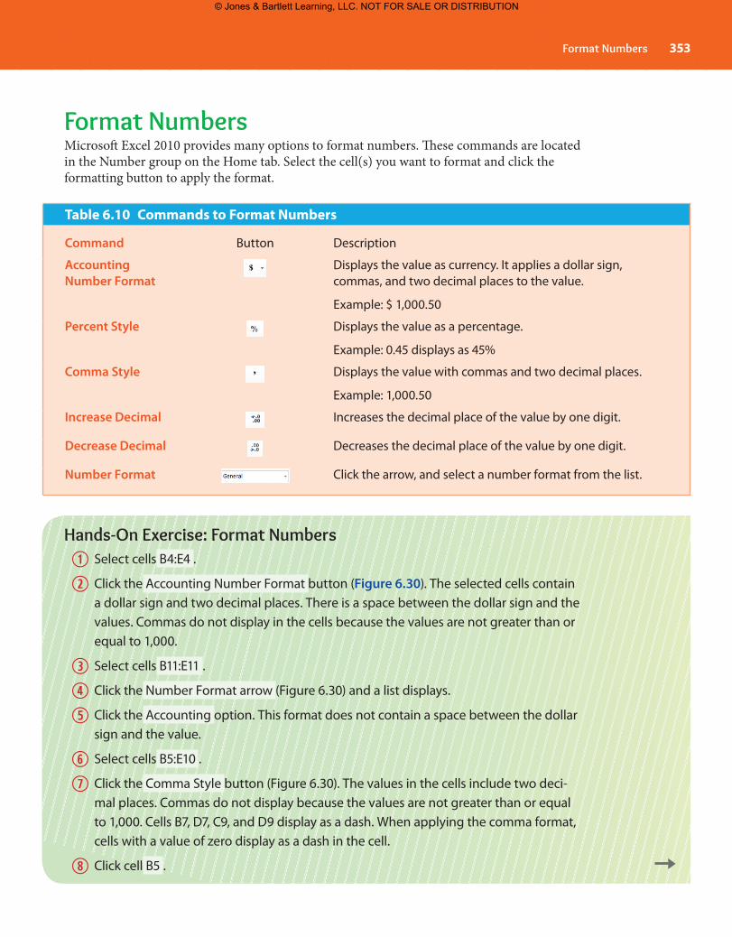
Format NumbersMicrosoft Excel 2010 provides many options to format numbers. Th ese commands are located in the Number group on the Home tab. Select the cell(s) you want to format and click the formatting button to apply the format.

Table 6.10 Commands to Format Numbers

Command Button Description

Accounting

Number Format

Displays the value as currency. It applies a dollar sign, commas, and two decimal places to the value.

Example: $ 1,000.50

Percent Style Displays the value as a percentage.

Example: 0.45 displays as 45%

Comma Style Displays the value with commas and two decimal places.

Example: 1,000.50

Increase Decimal Increases the decimal place of the value by one digit.

Decrease Decimal Decreases the decimal place of the value by one digit.

Number Format Click the arrow, and select a number format from the list.

Hands-On Exercise: Format Numbers

① Select cells B4:E4 .

② Click the Accounting Number Format button (Figure 6.30). The selected cells contain a dollar sign and two decimal places. There is a space between the dollar sign and the values. Commas do not display in the cells because the values are not greater than or equal to 1,000.

③ Select cells B11:E11 .

④ Click the Number Format arrow (Figure 6.30) and a list displays.

⑤ Click the Accounting option. This format does not contain a space between the dollar sign and the value.

⑥ Select cells B5:E10 .

⑦ Click the Comma Style button (Figure 6.30). The values in the cells include two deci-mal places. Commas do not display because the values are not greater than or equal to 1,000. Cells B7, D7, C9, and D9 display as a dash. When applying the comma format, cells with a value of zero display as a dash in the cell.

⑧ Click cell B5 .

Format Numbers 353



⑨ Click the Increase Decimal button (Figure 6.30). The value in the cell displays with three decimal places.

⑩ Click the Decrease Decimal button (Figure 6.30) and a decimal place is removed from the value. The value now contains two decimal places.

⑪ Click Save on the Quick Access Toolbar. The worksheet should resemble Figure 6.30.

Figure 6.30 Format Values

Accounting Number Format Number Format Decrease Decimal

Increase DecimalComma Style

Clear CommandTh e Clear command is used to delete the contents of a cell, delete the formatting of a cell, or both. It can also be used to clear comments and hyperlinks from a worksheet. Th e Clear button is located in the Editing group on the Home tab (Figure 6.31).

Use these steps to clear the contents or formatting of a cell:

• Click the cell that you want to clear.• Click the Clear button in the Editing group on the Home tab.• Click an option from the list.

Hands-On Exercise: Clear Formats and Contents of Cells

① Click cell A1 .

② Click the Clear button in the Editing group on the Home tab (Figure 6.31). A list of options display.




Modify Column and Row SizeOccasionally you will need to change the size of the columns or rows because the data is truncated (cut off ) in the cell or because you want to improve the readability or appearance of the cell.

If pound signs (####) display in a cell, that indicates that the column width is too small to fi t the contents of the cell. Th e column width can range from 0 to 255 characters. Th ese values represent the number of characters that can be displayed in a cell that is formatted with the

Figure 6.31 Clear Button

Clear

③ Click Clear All . The cell contents is deleted as well as the formatting. The cell is no longer merged.

④ Click Undo on the Quick Access Toolbar.

⑤ Click the Clear button.

⑥ Click Clear Formats . The formatting of the cell is removed, but the text remains in the cell.

⑦ Click Undo on the Quick Access Toolbar.

⑧ Click the Clear button.

⑨ Click Clear Contents . The contents of the cell are deleted.

⑩ Type Budget and press Enter . Notice that the formatting of the cell is still intact.

⑪ Click the Undo button twice to undo the last two steps. The worksheet should resem-ble Figure 6.31.

Modify Column and Row Size 355

79446_CH06_321-372.indd 5 06/12/12 8:36 PM user-f39979446_CH06_321-372.indd Page 355 06/12/12 8:36 PM user-f399 F-399F-399


standard default font. Th e default font for Microsoft Excel 2010 is Calibri, and the default font size is 11 points. Th e default column width is set at 8.43 characters. Th e column will be hidden if the column width is set to 0 characters. You can modify multiple column widths simultane-ously by selecting the columns before you modify the column size. Th e same holds true for modifying multiple row heights simultaneously.

Use any of these methods to modify the column width:

• Drag the right boundary of the column heading (Figure 6.32).• Double-click the right boundary of the column heading to automatically adjust the

column width to fi t the contents of the cell.• Right-click the column heading, and then click Column Width. Th e Column Width

dialog box displays. Type the width in the Column width box and click OK.• Click the column heading, click the Format button in the Cells group on the Home tab

(Figure 6.32), and then click Column Width. Th e Column Width dialog box displays. Type the width in the Column width box and click OK.

• To automatically increase the column width to fi t the contents of the cell, click the column heading, click the Format button in the Cells group on the Home tab, and then click AutoFit Column Width.

Th e default row height is 12.75 points. One point is approximately 1/72 inch. Th e row height can range from 0 to 409 points. If the row height is 0 points, the row will be hidden.

Use any of these methods to modify the row height:

• Drag the bottom boundary of the row heading (Figure 6.32).• Double-click the bottom boundary of the row heading to automatically adjust the row

height to fi t the contents of the cell.• Right-click the row heading and then click Row Height. Th e Row Height dialog box

displays. Type the height in the Row height box and click OK.• Click the row heading, click the Format button in the Cells group on the Home tab

(Figure 6.32), and then click Row Height. Th e Row Height dialog box displays. Type the height in the Row height box and click OK.

• To automatically increase the row height to fi t the cell contents, click the row heading, click the Format button in the Cells group of the Home tab, and then click AutoFit Row Height.

Hands-On Exercise: Modify Column and Row SizeReview the contents in column A. Notice that some of the text is not displaying. You will increase the size of the column in order to display all the cell contents.

① Right-click column A .

② Click Column Width . The Column Width dialog box displays.

③ Type 12 in the Column width box and click OK . All the text in the column now dis-plays in the cells.




Figure 6.32 Modify Column and Row Size

Right boundary of column C

Bottom boundary of row 16

Pound signs (####) display indicating that the columnwidth is too small to fit the entire contents of the cells

Format

④ Next, you will increase the row height for row 1.

a. Click row heading 1 to select the entire row.

b. Click the Format button in the Cells group on the Home tab (Figure 6.32).

c. Click Row Height . The Row Height dialog box displays.

d. Type 40 in the Row height box and click OK . The row height increases.

⑤ Next you will decrease the column width for column C.

a. Right-click column heading C .

b. Click Column Width . The Column Width dialog box displays.

c. Type 5 in the Column width box and click OK . Pound signs (####) display in the cells, which indicate that the column width is too small to fi t the contents (Figure 6.32). Whenever pound signs display, make certain to increase the column width to display all the contents in the cells.

⑥ To automatically increase the column width to view all the contents in column C, double-click the right boundary of column heading C (Figure 6.32). The contents in column C are displayed.

⑦ Click cell A1 . The worksheet will resemble Figure 6.33.

Modify Column and Row Size 357



Display FormulasUse one of the following methods to view the formulas entered in the worksheet:

• Press Ctrl � `. (Th e ` key is the key to the left of the number 1 on most keyboards.)• Click the Formulas tab, and then click the Show Formulas button in the Formula

Auditing group.

Th e formulas for the totals are displayed. To view the values again (the original default), press Ctrl � ` again or click the Show Formulas button.

Figure 6.33 Autofi t Contents of Column C

Hands-On Exercise: Display Formulas

① Click the Formulas tab (Figure 6.34).

② Click the Show Formulas button in the Formula Auditing group (Figure 6.34). The formulas display on the worksheet (Figure 6.34).

③ Click the Show Formulas button again. The values display on the worksheet.

④ Click Ctrl � ` to display the formulas. The formulas display on the worksheet.

⑤ Click Ctrl � ` to display the values.

⑥ Click the Home tab on the Ribbon to make it the active tab.




Check SpellingCheck a workbook for spelling errors before you print it. Th e Spelling button is located in the Proofi ng group on the Review tab (Figure 6.35). If you have multiple sheets in the workbook, you must check each worksheet. Before beginning the spell check, click the fi rst cell of the worksheet so the spell check can begin at the beginning of the worksheet.

Use these steps to check and correct spelling errors:

• Click the Review tab.• Click the Spelling button in the Proofi ng group, and the Spelling dialog box displays.

Th is feature checks the worksheet for errors and displays the errors in the dialog box. Some proper names may not be included in the dictionary and may display as a potential spelling error. In this case, click Ignore All to indicate that the word is spelled correctly or click Add to Dictionary to store it in the dictionary.

Figure 6.34 Display Formulas in Worksheet

Formulas Show Formulas

Hands-On Exercise: Check Spelling

① Click cell A1 .

② Click the Review tab.

③ Click the Spelling button. The Spelling dialog box displays if spelling errors exist.

④ Correct all spelling errors. If there are no spelling errors or after you have corrected all spelling errors, a dialog box displays stating that the spelling check is complete (Figure 6.35). Click OK .

⑤ Click the Home tab to make it the active tab.

⑥ Click Save on the Quick Access Toolbar.

Check Spelling 359



Print WorkbookYou can print the contents of the workbook or print the formulas in a workbook. By default, the workbook prints in portrait orientation. Portrait orientation is a page orientation that prints on a vertical page, which means that the page is taller than it is wide. You can change the page orientation to landscape orientation. Landscape orientation is a page orientation that prints on a horizontal page, which means that the page is wider than it is tall.

You can print the workbook from the Backstage view. You can also press Ctrl � P to display the Print command in the Backstage view. You have many print options.

• Select the number of copies to print.• Select a printer.• Select the print area (active sheet, entire workbook, selection).• Select the pages to print.• Select paper size (letter, legal, etc.).• Select page orientation (portrait or landscape).

Use these steps to print the workbook:

• Click the File tab.• Click Print.• Select Print Active Sheets in the Settings section to print the current active sheet in

the workbook (Figure 6.36), or you can click the Print Active Sheets button and select Print Entire Workbook to print the entire workbook.

• To print in landscape orientation, click the Portrait Orientation button and select Landscape Orientation (Figure 6.36).

• A preview of the worksheet displays on the right side of the window (Figure 6.36).

Spelling

Dialog box displays when spelling check is complete

Figure 6.35 Spelling Button

Portrait orien-tation: A page orientation that prints on a vertical page, which means that the page is taller than it is wide.

Landscape ori-entation: A page orientation that prints on a hori-zontal page, which means that the page is wider than it is tall.




• You can adjust the margins and other print settings as needed.• Click Print aft er you have selected all the print settings (Figure 6.36).

Use this step to print the formulas in the workbook:

• Press Ctrl � ` to view the formulas and then follow the same steps as listed above.

Hands-On Exercise: Print a Worksheet

① Click the File tab.

② Click Print . A preview of the printout displays on the right side of the window (Figure 6.36).

③ Select the printer you want to use (Figure 6.36).

④ Select Print Active Sheets in the Settings section (Figure 6.36).

⑤ Click the Print button (Figure 6.36).

Figure 6.36 Print Options

Print Copies

Select printer

Select page numbers

Select page orientation (portrait or landscape)

Select paper size

Select print area (Print Active Sheets or Entire Workbook)

Preview of printed worksheet

Page BreaksA page break is a dashed vertical and/or horizontal line in the worksheet that indicates where the worksheet is divided into separate pages. Th e page breaks display aft er the Print command is accessed from the Backstage view. Th e page breaks are determined based on paper size, margins, scale options, and the position of manual page breaks.

A dashed vertical line displays aft er column I (Figure 6.37). Th is indicates a page break. You can hide the page breaks when in Normal view if you need to.

Page break: A dashed vertical and/or horizontal line in the worksheet that indicates where the worksheet is divided into separate pages.

Page Breaks 361



Use these steps to hide page breaks in Normal view:

• Click the File tab.• Click Options and the Excel Options dialog box displays.• Click Advanced (Figure 6.38).• Click to remove the Show page breaks checkmark in the Display options for this

worksheet category (Figure 6.38). You may need to scroll down to fi nd this option.• Click OK.

Figure 6.37 Page Break

Page break

Figure 6.38 Remove Page Breaks

Advanced

Show page breaks




Help ButtonYou can use the Help feature if you need assistance with a task. The Help feature is accessed by clicking the Help button, which is located on the far-right corner of the Ribbon (Figure 6.39), or by pressing F1 on the keyboard. You can also access the Help command from the File tab.

Hands-On Exercise: Use Help

① Click the Help button, and the Excel Help dialog box displays (Figure 6.39).

② Type insert row in the Search box (Figure 6.39) and press Enter .

③ Search results display in the Excel Help dialog box (Figure 6.39). Click on a hyperlink to view the information.

④ Click the Print button in the Excel Help dialog box to print the information (Figure 6.39).

⑤ Click the Close button on the Excel Help dialog box (Figure 6.39).

Figure 6.39 Help Command

Search box PrintHelp

Close

Search results

Close a WorkbookYou should close the workbook when you are fi nished working with it. When you close a workbook, it will ask you to save if you have not done so already. Th is command does not close the application; it only closes the workbook.

Close a Workbook 363



To close a workbook:

• Click the File tab.• Click Close.• If the workbook has not been saved, it will prompt you to save the workbook at that

time.

You can also close the workbook by clicking the Close button on the Ribbon (Figure 6.40). If only one workbook is open in Microsoft Excel 2010, you can close the workbook and exit the application at once by clicking the Close button on the title bar or double-clicking the Microsoft Excel 2010 application icon (Figure 6.40). If multiple workbooks are open, these commands would close only the active workbook.

Hands-On Exercise: Close a Workbook

① Click the Close button on the Ribbon (Figure 6.40).

② The workbook closes but the application remains open.

Exit ApplicationUse the Exit command to exit the application. Th e Exit command is located on the File tab, or it can be accessed by pressing Alt � F4. You can also close the application by clicking the Close button on the title bar if only one workbook is open.

Figure 6.40 Close Commands

Microsoft Excel 2010 application icon Close button on title bar

Close button on Ribbon




Multiple-Choice Questions

1. Microsoft Excel 2010 is a application.a. Presentation graphics

b. Word processing

c. Spreadsheet

d. Database

2. Which of the following is true about the boundary of a row?a. Double-click the bottom boundary of a row to add a row.

b. Click the bottom boundary of a row and press Delete on your keyboard to delete a row.

c. Drag the bottom boundary of a row to change the height of the row.

d. Double-click the bottom boundary of a row to delete a row.

3. Press to edit the contents of a cell.a. F5

b. F2

c. Ctrl � Alt � Delete

d. Esc

4. By default, a workbook contains sheet(s).a. One

b. Two

c. Three

d. Five

5. By dragging the fi ll handle, you can cells.a. Move

b. Delete

c. Copy

d. Edit

6. Which of the following is an invalid cell reference?a. 100A

b. C55

c. az1000

d. za1

Hands-On Exercise: Exit Application

① Click the File tab.

② Click Exit and the application closes.

Exit Application 365



7. The function is used to total numbers in a workbook.a. Total

b. Sum

c. Calculate

d. Formula

8. If cell A3 contains the value 1050 and you change the format to comma style, how would the data display in the cell?a. 1,050

b. 1,050.00

c. $1,050

d. $1,050.00

9. The fi le extension of a Microsoft Excel 2010 workbook is .a. excel

b. xlsx

c. xls

d. excel2010

10. Press to view the formulas in the worksheet.a. Ctrl�Enter

b. Alt�Enter

c. F1

d. Ctrl�̀

Project #1: Create a Workbook Displaying the Costs of Vacation PackagesYou work for a travel agency and need to prepare a listing of all the vacation packages for the summer. You will use Microsoft Excel 2010 to accomplish this task.

① Set the column width of column A to 20.

② Enter the data from Figure 6.41 in the worksheet.

Figure 6.41 Enter Data in Worksheet




③ Merge and center cells A1 through B1.

④ Make the following changes to A1:

a. Bold

b. Font color � Blue

c. Font size � 18

⑤ Make the following format changes:

a. Bold cells A3 and B3.

b. Increase indent of cells B4:B7.

c. Format cells B4:B7 as Accounting Number Format.

⑥ Insert a row at row 6.

⑦ Add the following data to the cells:

a. Type European Cruise in cell A6.

b. Type 2000 in cell B6.

⑧ Spell-check the workbook and correct any mistakes.

⑨ Save the workbook as Paradise Travel. The worksheet should resemble Figure 6.42.

⑩ Delete row 5.

⑪ Save the workbook as Paradise Travel Revised. The worksheet should resemble Figure 6.43.

⑫ Print the workbook in landscape orientation.

⑬ Close the workbook.

Figure 6.42 Paradise Travel Workbook




Figure 6.43 Paradise Travel Revised Workbook

Project #2: Create a Workbook for a Law Firm to Track Hours Worked Weekly for Each ClientYour boss needs to track the hours he spends weekly on each of his clients. Th is information is used to process the client invoices each month. You will use Microsoft Excel 2010 to keep track of his hours.

① Create the worksheet in Figure 6.44.

Figure 6.44 Enter Text in Worksheet

② Merge and center A1 through F1.

③ Type Week 1 in cell B3.

④ Make the following changes to A1:

a. Bold

b. Font color � Blue, Accent 1

c. Font size � 28

d. Fill color � White, Background 1, Darker 15%

⑤ Change the column width of column A to 20.

⑥ Using the fi ll handle, copy cell B3 to cells C3 through E3 to complete the series. The text Week 2, Week 3, and Week 4 will be displayed in the cells.




⑦ Add the following data to the cells:



c. Type 10 in cell D4.

d. Type 5 in cell E4.

e. Type 14 in cell B5.

f. Type 7 in cell C5.

g. Type 20 in cell D5.

h. Type 20 in cell E5.

i. Type 12 in cell B6.

j. Type 18 in cell C6.

k. Type 10 in cell D6.

l. Type 15 in cell E6.

m. Type Total in cell F3.

⑧ Calculate the totals in cells F4:F6. The total should be the sum of the hours for each client.

⑨ Calculate the totals in cells B7:F7. The totals should be the sum of the hours for each week.

⑩ Apply the following formats:

a. Bold the cells in A3:F3.

b. Italicize cells A4:A6.

c. Increase indent of cells A4:A6.

d. Format cells B4:F7 as comma style.

e. Add a top and double bottom border around cells A7:F7.

⑪ Insert a row below row 6 and add the following data:

a. Type Georgia’s Hair Salon in cell A7.

b. Type 2 in cells B7, C7, D7, and E7.

c. Calculate the total for Georgia’s Hair Salon in cell F7.

⑫ Spell-check the worksheet and correct any mistakes.

⑬ Save the workbook as Orland Law Firm. The worksheet should resemble Figure 6.45.

⑭ Print the worksheet.

⑮ Print the worksheet with the formulas.

⑯ Change the client name in cell A4 to JK Sporting Goods.




⑰ Change the row height of row 8 to 24.

⑱ Delete row 6.

⑲ Save the workbook as Orland Law Firm Revised. The worksheet should resemble Figure 6.46.

⑳ Print the worksheet.

21 Close the workbook.

Figure 6.45 Orland Law Firm Workbook

Figure 6.46 Orland Law Firm Revised Workbook

Project #3: Create a Workbook to Calculate the Quarter Sales for a CompanyYou work for Pedro Electronics. You will use Microsoft Excel 2010 to keep track of the fi rst quarter sales for the company.

① Create the worksheet in Figure 6.47.




② Merge and center cells A1 through E1.

③ Merge and center cells A2 through E2.

④ Make the following changes to cells A1 and A2:

a. Bold

b. Font color � Green

c. Font size � 22

d. Fill color � White, Background 1, Darker 15%

⑤ Change the column width of column A to 15.

⑥ Change the column widths of columns B, C, D, and E to 12.

⑦ Using the fi ll handle, copy cell B4 to C4:D4 to complete the series. The text February and March will be displayed in the cells.

⑧ Add the following data to cells B5:D9 (Figure 6.48):

Figure 6.47 Enter Text

Figure 6.48 Enter Values

⑨ Type Total in cell E4.

⑩ Type Total in cell A10.




⑪ Calculate the totals in cells E5:E9. The totals are the sum of the monthly sales for each product.

⑫ Calculate the totals in cells B10:E10. The totals are the sum of the sales for each month.

⑬ Make the following format changes:

a. Bold cells A4:E4.

b. Bold cell A10.

c. Right-align cells B4:E4.

d. Italicize cells A5:A9.

e. Indent cells A5:A9.

f. Format cells B6:E9 as comma style. Decrease decimal places so that none are displayed.

g. Format cells B5:E5 and B10:E10 as Accounting Number Format. Decrease decimal places so that no decimal places are displayed.

h. Add a top and double bottom border around cells A10:E10.

⑭ Spell-check the worksheet and correct any mistakes.

⑮ Save the workbook as Pedro Electronics. The worksheet should resemble Figure 6.49.

⑯ Print the worksheet.

⑰ Print the worksheet with the formulas.

⑱ Close the workbook.

⑲ Exit Microsoft Excel 2010.

Figure 6.49 Pedro Electronics Workbook




Create Workbooks Using Microsoft Excel 2010 - Jones & Bartlett

Documents

Transcript of Create Workbooks Using Microsoft Excel 2010 - Jones & Bartlett