1

1

CSC 4103 - Operating Systems

Spring 2007

Tevfik Koşar

Louisiana State University

February 1st, 2007

Lecture - V

CPU Scheduling

2

Roadmap

• CPU Scheduling

– Basic Concepts

– Scheduling Criteria

– Different Scheduling Algorithms

2

3

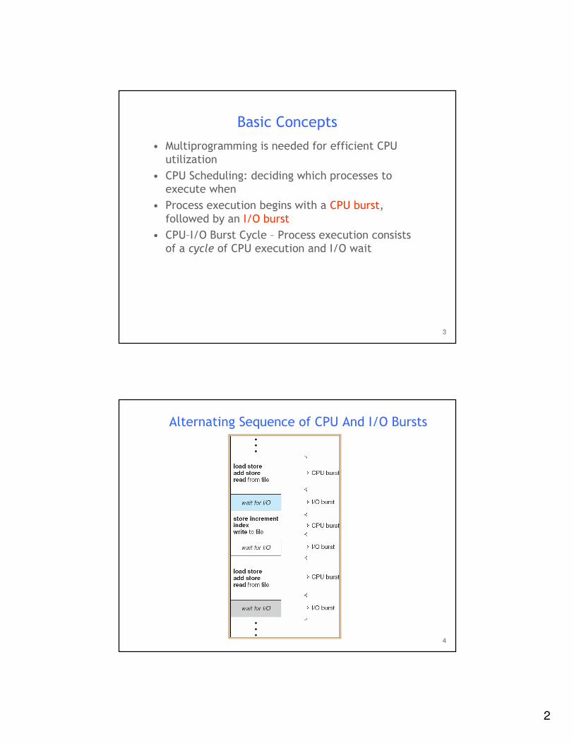
Basic Concepts

• Multiprogramming is needed for efficient CPU

utilization

• CPU Scheduling: deciding which processes to execute when

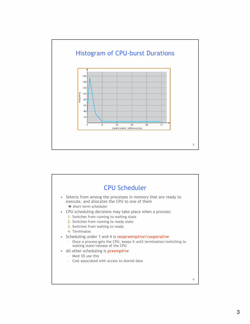
• Process execution begins with a CPU burst,

followed by an I/O burst

• CPU–I/O Burst Cycle – Process execution consists of a cycle of CPU execution and I/O wait

4

Alternating Sequence of CPU And I/O Bursts

3

5

Histogram of CPU-burst Durations

6

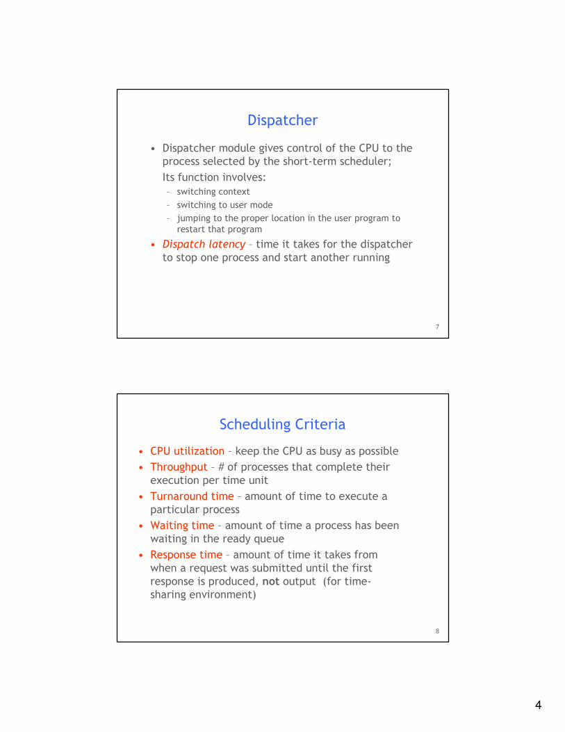
CPU Scheduler

• Selects from among the processes in memory that are ready to execute, and allocates the CPU to one of them

� short-term scheduler

• CPU scheduling decisions may take place when a process:

1. Switches from running to waiting state

2. Switches from running to ready state

3. Switches from waiting to ready

4. Terminates

• Scheduling under 1 and 4 is nonpreemptive/cooperative

– Once a process gets the CPU, keeps it until termination/switching to waiting state/release of the CPU

• All other scheduling is preemptive

– Most OS use this

– Cost associated with access to shared data

4

7

Dispatcher

• Dispatcher module gives control of the CPU to the process selected by the short-term scheduler;

Its function involves:

– switching context

– switching to user mode

– jumping to the proper location in the user program to

restart that program

• Dispatch latency – time it takes for the dispatcher

to stop one process and start another running

8

Scheduling Criteria

• CPU utilization – keep the CPU as busy as possible

• Throughput – # of processes that complete their

execution per time unit

• Turnaround time – amount of time to execute a

particular process

• Waiting time – amount of time a process has been

waiting in the ready queue

• Response time – amount of time it takes from

when a request was submitted until the first

response is produced, not output (for time-sharing environment)

5

9

Optimization Criteria

• Max CPU utilization

• Max throughput

• Min turnaround time

• Min waiting time

• Min response time

10

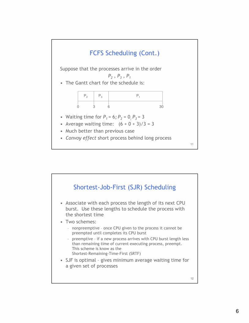
First-Come, First-Served (FCFS) Scheduling

Process Burst Time

P1 24

P2 3

P3 3

• Suppose that the processes arrive in the order: P1 , P2 , P3

The Gantt Chart for the schedule is:

• Waiting time for P1 = 0; P2 = 24; P3 = 27

• Average waiting time: (0 + 24 + 27)/3 = 17

P1 P2 P3

24 27 300

6

11

FCFS Scheduling (Cont.)

Suppose that the processes arrive in the order

P2 , P3 , P1

• The Gantt chart for the schedule is:

• Waiting time for P1 = 6; P2 = 0; P3 = 3

• Average waiting time: (6 + 0 + 3)/3 = 3

• Much better than previous case

• Convoy effect short process behind long process

P1P3P2

63 300

12

Shortest-Job-First (SJR) Scheduling

• Associate with each process the length of its next CPU

burst. Use these lengths to schedule the process with the shortest time

• Two schemes:

– nonpreemptive – once CPU given to the process it cannot be

preempted until completes its CPU burst

– preemptive – if a new process arrives with CPU burst length less

than remaining time of current executing process, preempt.

This scheme is know as the

Shortest-Remaining-Time-First (SRTF)

• SJF is optimal – gives minimum average waiting time for a given set of processes

7

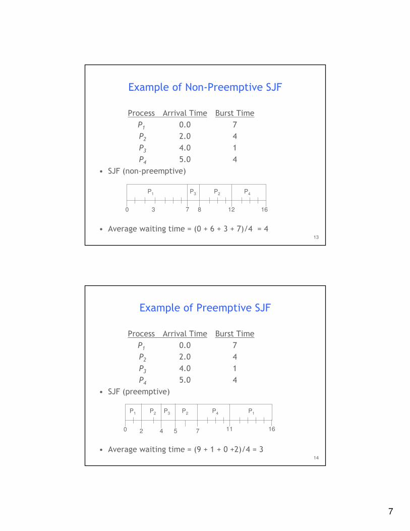
13

Process Arrival Time Burst Time

P1 0.0 7

P2 2.0 4

P3 4.0 1

P4 5.0 4

• SJF (non-preemptive)

• Average waiting time = (0 + 6 + 3 + 7)/4 = 4

Example of Non-Preemptive SJF

P1 P3 P2

73 160

P4

8 12

14

Example of Preemptive SJF

Process Arrival Time Burst Time

P1 0.0 7

P2 2.0 4

P3 4.0 1

P4 5.0 4

• SJF (preemptive)

• Average waiting time = (9 + 1 + 0 +2)/4 = 3

P1 P3P2

42 110

P4

5 7

P2 P1

16

8

15

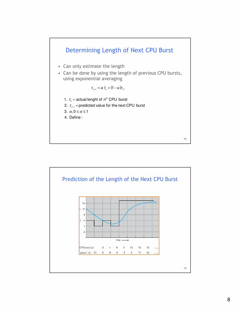
Determining Length of Next CPU Burst

• Can only estimate the length

• Can be done by using the length of previous CPU bursts, using exponential averaging

:Define 4.

10 , 3.

burst CPU next the for value predicted 2.

burst CPU of lenght actual 1.

1

≤≤

=

=

+

αα

τn

th

nnt

( ) .1 1 nnn

t ταατ −+==

16

Prediction of the Length of the Next CPU Burst

9

17

Examples of Exponential Averaging

• α =0– τn+1 = τn– Recent history does not count

• α =1– τn+1 = α tn– Only the actual last CPU burst counts

• If we expand the formula, we get:τn+1 = α tn+(1 - α)α tn -1 + …

+(1 - α )j α tn -j + …

+(1 - α )n +1 τ0

• Since both α and (1 - α) are less than or equal to 1, each successive term has less weight than its predecessor

18

Priority Scheduling

• A priority number (integer) is associated with each

process

• The CPU is allocated to the process with the highest

priority (smallest integer ≡ highest priority)

– Preemptive

– nonpreemptive

• SJF is a priority scheduling where priority is the predicted next CPU burst time

• Problem ≡ Starvation – low priority processes may never execute

• Solution ≡ Aging – as time progresses increase the priority of the process

10

19

Round Robin (RR)

• Each process gets a small unit of CPU time

(time quantum), usually 10-100 milliseconds.

After this time has elapsed, the process is

preempted and added to the end of the ready queue.

• If there are n processes in the ready queue and

the time quantum is q, then each process gets

1/n of the CPU time in chunks of at most q

time units at once. No process waits more than (n-1)q time units.

• Performance

– q large ⇒ FIFO

– q small ⇒ q must be large with respect to context switch, otherwise overhead is too high

20

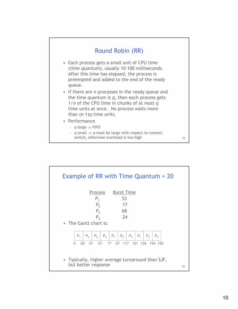
Example of RR with Time Quantum = 20

Process Burst Time

P1 53

P2 17

P3 68

P4 24

• The Gantt chart is:

• Typically, higher average turnaround than SJF, but better response

P1 P2 P3 P4 P1 P3 P4 P1 P3 P3

0 20 37 57 77 97 117 121 134 154 162

11

21

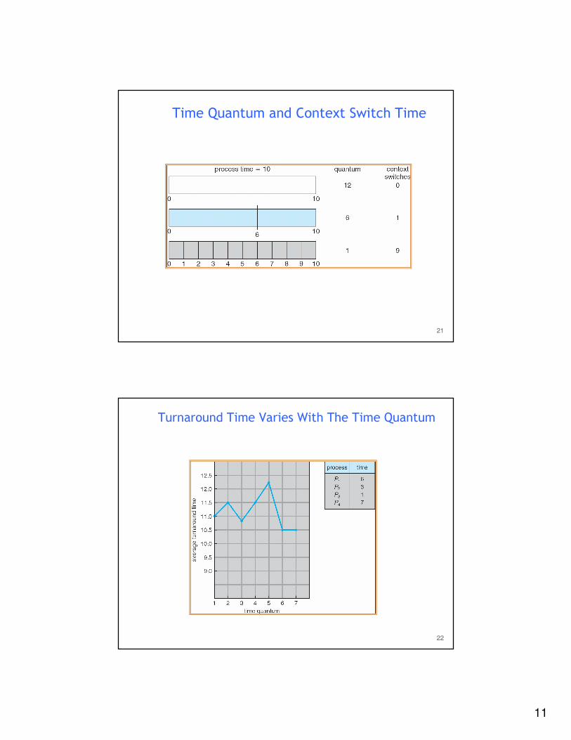
Time Quantum and Context Switch Time

22

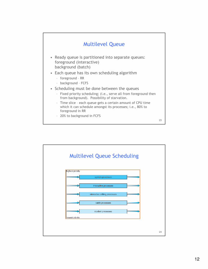
Turnaround Time Varies With The Time Quantum

12

23

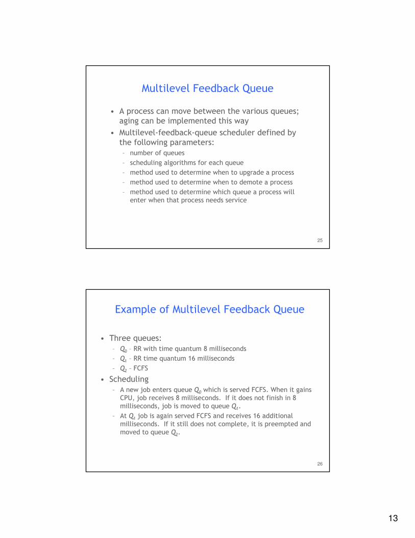
Multilevel Queue

• Ready queue is partitioned into separate queues:

foreground (interactive)background (batch)

• Each queue has its own scheduling algorithm

– foreground – RR

– background – FCFS

• Scheduling must be done between the queues

– Fixed priority scheduling; (i.e., serve all from foreground then

from background). Possibility of starvation.

– Time slice – each queue gets a certain amount of CPU time

which it can schedule amongst its processes; i.e., 80% to

foreground in RR

– 20% to background in FCFS

24

Multilevel Queue Scheduling

13

25

Multilevel Feedback Queue

• A process can move between the various queues; aging can be implemented this way

• Multilevel-feedback-queue scheduler defined by

the following parameters:

– number of queues

– scheduling algorithms for each queue

– method used to determine when to upgrade a process

– method used to determine when to demote a process

– method used to determine which queue a process will

enter when that process needs service

26

Example of Multilevel Feedback Queue

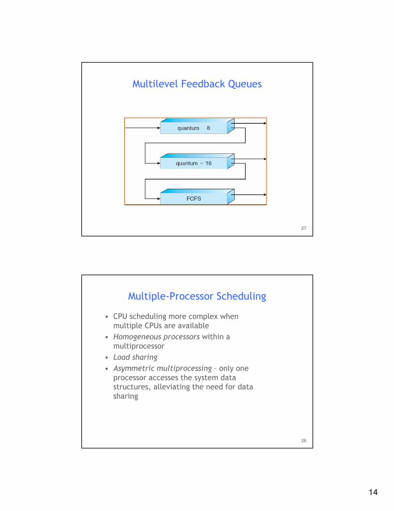
• Three queues:

– Q0 – RR with time quantum 8 milliseconds

– Q1 – RR time quantum 16 milliseconds

– Q2 – FCFS

• Scheduling

– A new job enters queue Q0 which is served FCFS. When it gains

CPU, job receives 8 milliseconds. If it does not finish in 8

milliseconds, job is moved to queue Q1.

– At Q1 job is again served FCFS and receives 16 additional

milliseconds. If it still does not complete, it is preempted and

moved to queue Q2.

14

27

Multilevel Feedback Queues

28

Multiple-Processor Scheduling

• CPU scheduling more complex when

multiple CPUs are available

• Homogeneous processors within a

multiprocessor

• Load sharing

• Asymmetric multiprocessing – only one

processor accesses the system data structures, alleviating the need for data

sharing

15

29

Real-Time Scheduling

• Hard real-time systems – required to complete a critical task within a

guaranteed amount of time

• Soft real-time computing – requires

that critical processes receive priority

over less fortunate ones

30

Thread Scheduling

• Local Scheduling – How the threads library decides

which thread to put onto an available LWP

• Global Scheduling – How the kernel decides which

kernel thread to run next

16

31

Pthread Scheduling API#include <pthread.h>

#include <stdio.h>

#define NUM THREADS 5

int main(int argc, char *argv[])

{

int i;

pthread t tid[NUM THREADS];

pthread attr t attr;

/* get the default attributes */

pthread attr init(&attr);

/* set the scheduling algorithm to PROCESS or SYSTEM */

pthread attr setscope(&attr, PTHREAD SCOPE SYSTEM);

/* set the scheduling policy - FIFO, RT, or OTHER */

pthread attr setschedpolicy(&attr, SCHED OTHER);

/* create the threads */

for (i = 0; i < NUM THREADS; i++)

pthread create(&tid[i],&attr,runner,NULL);

32

Pthread Scheduling API

/* now join on each thread */

for (i = 0; i < NUM THREADS; i++)

pthread join(tid[i], NULL);

}

/* Each thread will begin control in this function */

void *runner(void *param)

{

printf("I am a thread\n");

pthread exit(0);

}

17

33

Operating System Examples

• Solaris scheduling

• Windows XP scheduling

• Linux scheduling

34

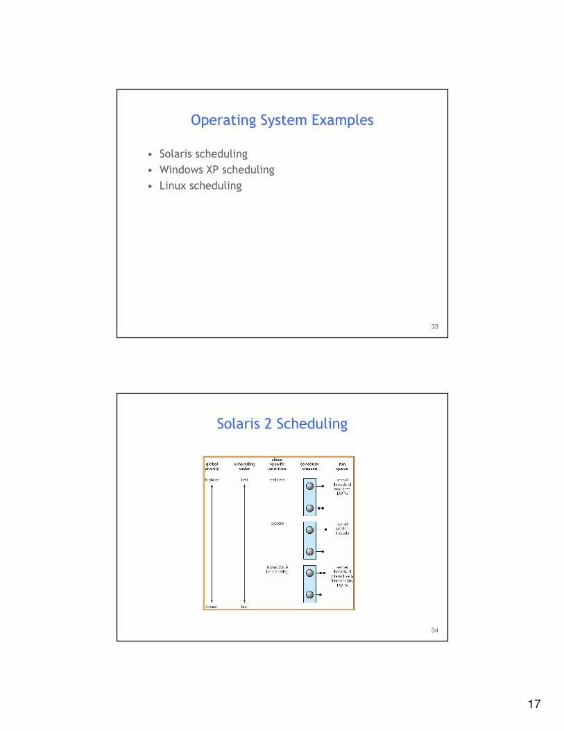
Solaris 2 Scheduling

18

35

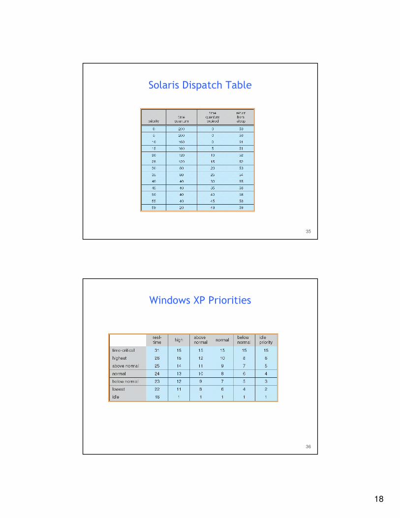
Solaris Dispatch Table

36

Windows XP Priorities

19

37

Linux Scheduling

• Two algorithms: time-sharing and real-time

• Time-sharing– Prioritized credit-based – process with most credits is scheduled next

– Credit subtracted when timer interrupt occurs

– When credit = 0, another process chosen

– When all processes have credit = 0, recrediting occurs

• Based on factors including priority and history

• Real-time– Soft real-time

– Posix.1b compliant – two classes

• FCFS and RR

• Highest priority process always runs first

38

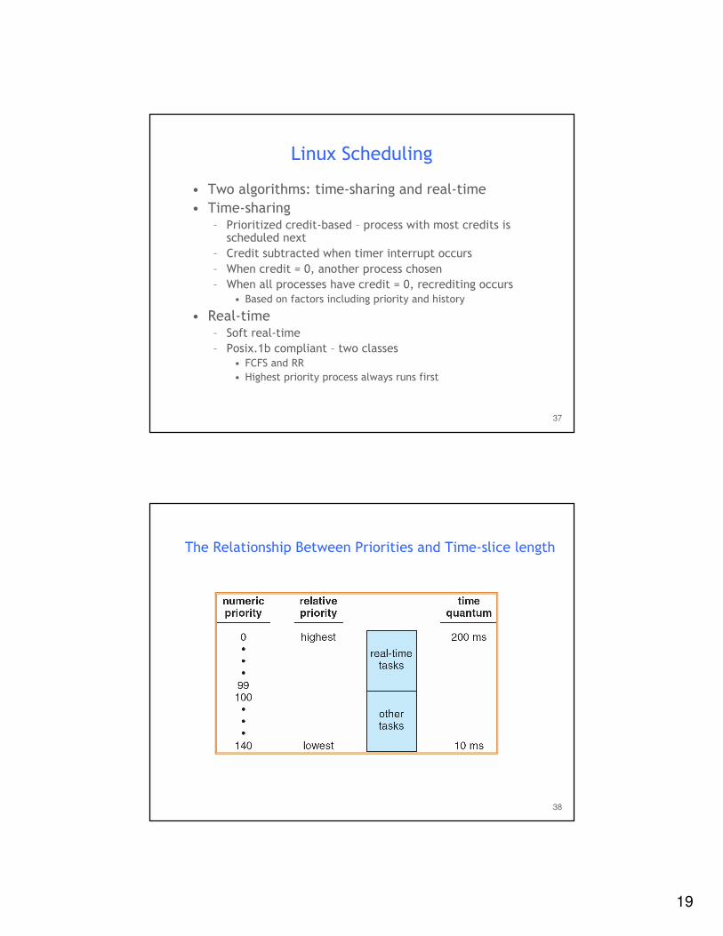
The Relationship Between Priorities and Time-slice length

20

39

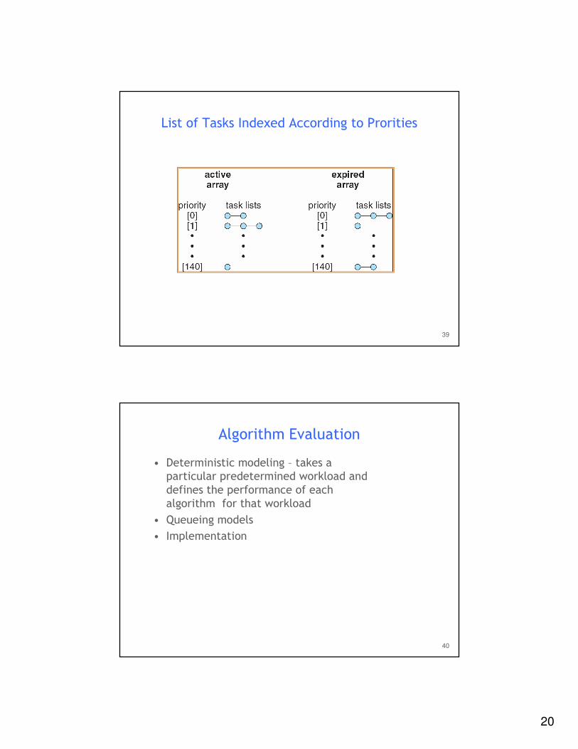
List of Tasks Indexed According to Prorities

40

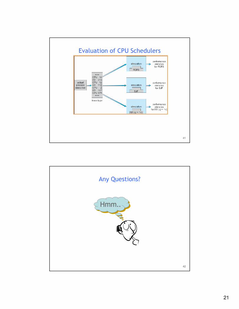
Algorithm Evaluation

• Deterministic modeling – takes a particular predetermined workload and

defines the performance of each

algorithm for that workload

• Queueing models

• Implementation

21

41

Evaluation of CPU Schedulers

42

Any Questions?

Hmm..Hmm..

22

43

Reading Assignment

• Read chapter 5 from Silberschatz.

44

Acknowledgements

• “Operating Systems Concepts” book and supplementary

material by Silberschatz, Galvin and Gagne.