CPN 503 Elite

HYDROPROBE™

OPERATING MANUAL

CPN International An InstroTek Company

Copyright © December 2013

V1.0

All Rights Reserved

No part of this manual may be reproduced for any purpose

without the written permission of InstroTek, Inc.

www.InstroTek.com

NOTE:

This Operating Manual applies only to

CPN 503 Elite software.

Table of Contents

General Information .......................................................... 1

Getting Started ................................................................... 8

Operation .......................................................................... 12

Maintenance .................................................................... 29

Operating Precautions ................................................... 33

Troubleshooting ................................................................ 34

Print Data/Transfers .......................................................... 36

Counting Statistics ........................................................... 37

Connector Pinouts ........................................................... 44

Front Panel USB ................................................................. 45

Excel Spreadsheet ........................................................... 45

Index ................................................................................... 46

General Information

1

Section 1 – General Information Congratulations on the purchase of your new CPN 503 Elite soil moisture gauge.

The Model CPN 503 Elite HYDROPROBE, NEUTRON MOISTURE PROBE, measures

the sub-surface moisture in soil and other materials by use of a probe containing

a source of high energy neutrons and a slow (thermal) neutron detector. The

probe is lowered into a pre-drilled and cased hole (1.5 or 2 inch diameter).

The source used in this gauge emits fast neutrons. Fast neutrons from the source

interact with Hydrogen in water and thermalize (slow down) neutrons. The

thermal or slow neutrons are then counted by the He3 tube. Increase in water

content results in a proportional increase in thermal neutron counts detected by

the tube. The moisture data is displayed directly in units of interest on the

electronic assembly which is connected to the source shield assembly.

This state-of-the-art instrument offers a simple to operate but superior alternative

to other methods of soil moisture monitoring. The operator needs minimal

instructions.

The probe is supplied with an 8 foot cable and ten adjustable cable stops.

Additional stops and longer cable lengths are available upon request.

Upon retraction of the probe into the shield, the probe latches automatically in

place for transportation and can be locked with a pad lock if necessary.

The complete assembly is supplied with a shipping and carrying container which

contains accessory items, cable, operating manual, and other materials which

the operator may wish to carry.

General Information

2

CPN 503 Elite Features

The CPN 503 Elite Direct Readout Model Provides:

Integral microprocessor for simple function selection.

Rapid, precise repeatable soil moisture measurements.

Light weight and portable.

Field service and component exchange with tools provided.

Storage and recall selection of linear calibrations for 32 soil or tubing

types.

Operator selected time of test, logging format and units of measurements.

Data transferred serially to a PC via a USB port using a USB 2.0 A-male to B-

male cable.

Data downloaded to a USB mass storage device (Thumb Drive).

General Information

3

Functional Description

The CPN 503 Elite HYDROPROBE® operates by emitting radiation from an

encapsulated radioactive source, Americium-241:Beryllium. To determine the

moisture content in the soil, the Americium-241:Beryllium source emits neutron

radiation into the soil under test. The high-energy neutrons are moderated by

colliding with hydrogen in the moisture of the soil. Only low-energy, moderated

neutrons are detected by the Helium-3 detector. A soil that is wet will give a high

count per time of test. A soil that is dry will give a low count for the same period

of time.

Figure 1.1 Operation of the 503 Elite HYDROPROBE®

Standard Equipment

General Information

4

Each 503 Elite is provided with a durable plastic shipping case and the items

shown listed below. There are no special instructions for unpacking the 503Elite

Hydroprobe ®. It comes fully assembled.

503 Elite Hydroprobe ®

Padlock with Keys

Shipping Case

8 ft. (2.44 meter) Cable

10 Cable Stops

Access Collar (1.5”)

Battery Pack (Installed)

Operating Manual

Leak Test Certificate

Figure 1.2 Standard Equipment

General Information

5

Specifications

Dimensions/Shipping Weights:

Model Weight Length Width Height

Gauge Only 15.7lbs (7.12kg) 7.0” (178mm) 6.8” (173mm) 14” (356mm)

Gauge & Carry

Case 36.5lbs (16.6kg) 13.0” (330mm) 24.0” (610mm) 10.0” (254mm)

Probe Weight Length Diameter

Model 2.0 2.3lbs (1.04kg) 12.7” (323mm) 1.86” (47.4mm)

Model 1.5 1.7lbs (0.77kg) 12.7” (323mm) 1.50” (38.1mm)

Performance

Function ............................................................... Sub-surface moisture measurements

Range .............. Linear calibration: 0 to 40% per volume, 0.40 g/cc, 25 pcf, 4.8 in/ft

Precision ..........................................................0.24% at 24% per volume at one minute

Count Time ........................................................ User selectable from 1 to 960 seconds

Display ....................................................... 4 lines x 20 character Liquid Crystal Display

Data

Storage ................................................................................................ 2 GB of storage

Format ................................................................................ Operator programmable

Notes .................................................................... 0-99 notes of 19 characters each

Counts ..................................................................................... 0-99 counts per record

Data Output ......................... USB A-B Male Cable download to personal computer

Calibration ........................................................................ 32 user programmed (linear)

Units ........................................................................... in/ft, pcf, g/cc, %Moist, cm/30cm

Construction

Body: ......................................... Aluminum with epoxy paint & hard-anodize finish

Wear Parts: .............................................................................................. Stainless Steel

General Information

6

Specifications

Electrical

Power

Lithium .................................................................. Li-Ion 7.4V 4400mAh Battery Pack

Battery Life .................................................................................... Approximately 2 years

Consumption .......................................................................................... 6.5 mA Average

Environmental

Operating Temperature

Ambient .............................................................................. 32º to 150º F (0º to 66º C)

Storage .............................................................................. -4º to 140º F (-20º to 60º C)

Humidity (Non-Condensing) ..................................................................................... 95%

Radiological

Neutron Source .................... Maximum 1.85 GBq (50 mCi) Americium-241:Beryllium

Encapsulation ............................................................ Double-sealed capsule CPN-131

Shielding ......................................................................................... Silicon-Based Paraffin

Shipping Requirements

UN3332, Radioactive Material

Type A Package, Special form 7

Transport index 0.2

Yellow II label, RQ

Special Form Approval ........................................................... USA/0627/S or CZ/1009/S

An NRC or agreement state license is required for domestic use. Contact CPN -

InstroTek for assistance in obtaining training for a license.

CPN - InstroTek reserves the right to change equipment specifications and/or design to

meet industry requirements or improve product performance.

General Information

7

CPN 503 Elite HYDROPROBE® Inspection

To familiarize yourself with the CPN 503 Elite DR HYDROPROBE®, perform the following

review.

1. Remove the HYDROPROBE® from the shipping case

and place it on a solid flat surface, such as a concrete

floor.

2. Examine the keyboard, the display screen, the cable,

probe, and shield box.

NOTE

The radioactive source is located at the

bottom part of the probe.

Do not touch this part of the probe or

place yourself in front of it.

3. Cable Stops

The gauge is supplied with ten each clamp-on cable stops. This will allow taking

measurements at half foot increments in a root zone up to five feet deep. For a deeper

root zone or for smaller increments, order more stops. Figure 1.4 shows a cross-section of

the gauge. Use it to position the first stop so that the measurement point on the probe

(as indicated by the band) is in the middle of the top foot of the root zone. Its actual

location will depend upon how high the access tubes stick out of the soil. Install all

tubes to the same height.

For example, if the base of the gauge is 5.0 inches above

the soils, and you want to take the first measurement at 6

inches, place the stop at 5.35 + 5.0 + 6.0 =16.35 inches

above the stop reference line.

4. Tube Adapter Ring

The bottom of the gauge contains an oversize hole to allow

inserting an adapter ring with a diameter to match the type

of access tubing being used. The ring is secured by a screw

through the front of the casting. Unless specified otherwise

at the time of order, an adapter ring for aluminum tubing

will be supplied. Adapter rings for other types (e.g.

diameters) are available from CPN –InstroTek, Inc. or can be

constructed locally. Figure 1.4 503DR Cross Section

Figure 1.3 CPN 503DR HYDROPROBE®

Getting Started

8

Section 2 – Getting Started

The CPN 503 Elite includes an updated keypad interface with menu related

function keys.

Key Function

Start/Enter Take a reading and select from drop down menu functions

On/Off Power on/off function

No

Yes

Function key for software/menu requests

Function key for software/menu requests

Store Store Data to connected USB device

Time Enter count time for the length of a reading

Esc Escape key used to return to main menu or previous screen

Yes Function key for software/menu requests.

STD Select Standard Count menu

Menu 14 Item gauge control functions

Arrow Keys Navigate through the menus

The operator must set the probe to a configuration to meet the field conditions.

To assist in understanding the gauge initially, it is shipped from the factory in the

following configuration.

The initial setting may be accessed by pushing MENU or (Front Panel Key)

8-UNITS 3-Inches per foot.

(TIME) 15 second.

14CALIB CAL #0 Factory calibration in saturated and dry sand.

Coefficient A (slope) approx. 2.5 in/ft. and

Coefficient B (intercept) approx. –0.06 in/ft.

(STD) Standard count approx. 4000

With the gauge sitting on the top of the shipping case, press STD the gauge will

prompt you to take a new Standard Count; press YES. The count lasts 256

seconds and should be taken once a day.

Getting Started

9

Figure 2.1 CPN 503 Elite Keyboard

To change from Inches/foot to %Moisture:

PRESS MENU – use Arrow keys to navigate to Item 7- Select Units

PRESS ENTER - use Arrow keys to navigate to Item 5- % Moist

PRESS ENTER

PRESS ESC

Take another count by pressing START. The measured result should be the same

as above except that the count should take 15 seconds and the display should

be approximately 20.0% moisture by volume (which is equivalent to 2.4 inches

per foot in the reading above).

Keyboard MENU Controls and Display

Getting Started

10

Most functions are directly entered by pressing MENU. Options are chosen by

the arrow keys and selected with ENTER. Test Results are viewed by using the

up/down arrows after pushing START.

Menu Function

MC Moisture Count: Raw gauge counts/unit time

R Ratio: MC/Standard Count= Ratio

Units (7) Select Units

%Moist Water content ( vol. %) = a * count ratio + b

g/cc grams of water/ cubic cm of soil

lb/cf pounds of water/cubic foot of soil

in/ft inches of water/ft of soil

cm/30cm centimeters of water/30 cm of soil

TIME Select counting time (1 to 960) seconds.

CALIB(12)

(1) Select calibration (0…32)

(2) Enter/Change

(3) View Calibration

(4) Send to USB

(5) Send to Serial

(6) Load from USB

Project(4)

User defined measurement/site information. Contains

Calibration, tube/count time information depths. Projects

required to log readings outside of daily log

Logging(11) Functions 1-6 Start, Change Log Time (1-999sec), Change #

Logs (1-999), View, Send

Getting Started

11

Recall (1) Recall Last Test

PRINT Menu selection (STD,2,3,13,14) Serial USB Connection to

Device.

MENU Select miscellaneous function:

STD 1-4 Standard Count New, Review, Send USB or Serial

START Take a reading.

NO CLEAR, Abort, No

STORE Store Reading in Daily Log or Project

ENTER Enter data, make selection

Operation

12

Section 3 - Operation

Operating Procedures

Taking A Reading (Standard Count Required to Calculate Moisture)

To take a reading, lower the probe to

the appropriate depth and press START.

Before doing this you must select UNITS,

TIME and CALIBRATION or PROJECT.

Note: The gauge must have a valid

standard count to function correctly.

How to Select UNITS (MENU item 8)

The choice of display units will depend

upon your use. Researchers will

normally prefer grams per cubic

centimeter or percent volume, while

irrigation schedulers use inches per foot

or centimeter per 30 centimeters. Figure 3.1 Operation of the 503 Elite HYDROPROBE®

Counts are used for downloading to a software program and are helpful for

troubleshooting. It is the same data, only differing by the conversion factor.

Once the units have been selected, then each time a Count is taken, the

display will be in the units selected.

How to Select TIME (Select from Front Panel 1-960 seconds)

For a given counting rate, the counting time interval determines the precision of

the measurement. The longer the time selected, the more precise the

measurement. Correspondingly, the longer the counting times the fewer

measurements that can be made in a day. Thus the time interval is normally

selected as the minimum time that will meet your specific precision.

For scheduling-type operation, a count time of 16 seconds will provide sufficient

precision for irrigation scheduling.

See the appendix section on Counting Statistics for a further discussion of

precision.

Operation

13

How to Select CALIBRATION (MENU item 14 1-32)

The calibration will have been determined previously, and the slope (A) and

intercept (B) coefficients stored in one of the 32 calibrations. Select the one that

is appropriate for the soil and type of access tube.

Operating Procedures

To Log Readings (Press STORE after completion of reading if not using Auto Store)

Readings can be logged by the gauge as they are taken in the field or pre-set

with count time and number of readings/logs per location. Each tube site

represents a record of information. Prior to storing any readings, you must define

the format of the tube site record. After readings have been logged, they may

be recalled for display or downloaded to an external device.

There are 4 ways to log data with the 503 Elite.

1. Daily log

2. Simple Project

3. Full Project

4. Continuous Logging

Each will be described in detail below.

Daily Log

The results are shown after taking a reading. Pressing STORE form this screen will

prompt you with:

Pressing YES here will save the results in a log

called ‘Daily Log’ under the date the log was

taken.

Note: All projects must be deactivated to use

the Daily Log.

Operation

14

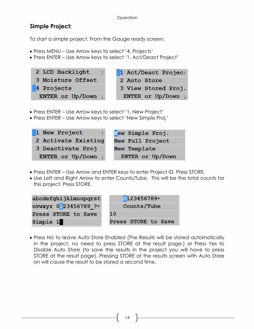
Simple Project:

To start a simple project, From the Gauge ready screen:

Press MENU – Use Arrow keys to select ‘4. Projects‘

Press ENTER – Use Arrow keys to select ‘1. Act/Deact Project’

Press ENTER – Use Arrow keys to select ‘1. New Project’

Press ENTER – Use Arrow keys to select ‘New Simple Proj.’

Press ENTER – Use Arrow and ENTER keys to enter Project ID. Press STORE.

Use Left and Right Arrow to enter Counts/Tube. This will be the total counts for

this project. Press STORE.

Press No to leave Auto Store Enabled (The Results will be stored automatically

in the project, no need to press STORE at the result page.) or Press Yes to

Disable Auto Store (to save the results in the project you will have to press

STORE at the result page). Pressing STORE at the results screen with Auto Store

on will cause the result to be stored a second time.

Operation

15

Press YES at the Accept Screen if the data is correct. Notice the A on the

Gauge Ready Screen, it signifies that you have chosen Auto Store.

Press START from this screen to take a test. You will be prompted to enter notes

at the beginning of each tube. Press YES to enter any notes. Press NO and the

test will begin.

After the test finishes the result screen is shown. Pressing START from here will

run another test. Pressing STORE will save the results again.

Full Project Template:

The Full project would be used in a situation where you have a static setup with

2 or more fields and a known number of tubes. This example contains 2 fields

with different number of tubes, readings and calibration constants.

Operation

16

To setup a full Project you must first setup a template.

From the Gauge Ready screen:

Press MENU – Use the Arrow keys to select ‘4. Projects’

Press ENTER – Use Arrow keys to select ‘1. Act/Deact Project’

Press ENTER – Use Arrow keys to select ‘1. New Project’

Press ENTER – Use Arrow keys to select ‘New Template’ Press ENTER

Use Arrow and ENTER keys to enter Template ID. Press STORE.

Use Left and Right Arrow to enter the number of stations, 2 in this example.

Use Arrow and ENTER keys to enter Station 1 ID. Press STORE.

Use Left and Right Arrow to enter the number of tubes at this station, 5 in this

example.

Operation

17

Use Arrow and ENTER keys to enter Tube 1 ID. Press STORE.

Use Left and Right Arrow to enter the number of readings for this tube.

Use UP/DOWN keys to select the calibration constant for this tube. Each tube

can have a different calibration constant.

Repeat from enter Tube ID for the remaining 4 tubes.

Repeat from enter Station ID for the Field 2.

When you are finished you will be presented with the accept screen. Press YES if

all the data is correct

Full Project:

Once the template has been created, you can select it for a new Full Project.

Press MENU – Use Arrow keys to select ‘4. Projects‘

Press ENTER – Use Arrow keys to select ‘1. Act/Deact Project’

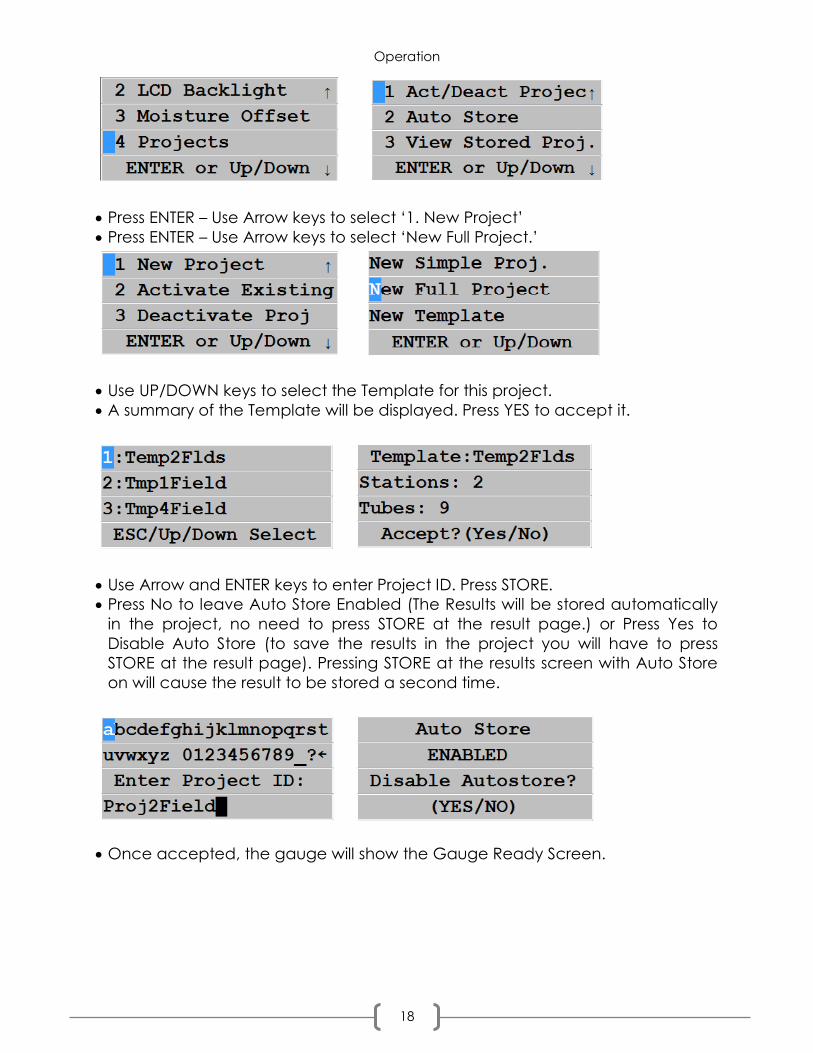
Operation

18

Press ENTER – Use Arrow keys to select ‘1. New Project’

Press ENTER – Use Arrow keys to select ‘New Full Project.’

Use UP/DOWN keys to select the Template for this project.

A summary of the Template will be displayed. Press YES to accept it.

Use Arrow and ENTER keys to enter Project ID. Press STORE.

Press No to leave Auto Store Enabled (The Results will be stored automatically

in the project, no need to press STORE at the result page.) or Press Yes to

Disable Auto Store (to save the results in the project you will have to press

STORE at the result page). Pressing STORE at the results screen with Auto Store

on will cause the result to be stored a second time.

Once accepted, the gauge will show the Gauge Ready Screen.

Operation

19

Press START from this screen to take a test. You will be prompted to enter notes

at the beginning of each tube. Press YES to enter any notes. Press NO and the

test will begin.

After the test finishes the result screen is shown. Pressing START from here will

run another test. Pressing STORE will save the results again

How to format Continuous Logging

Use the MENU key item (12) Logging to format the data storage area to agree

with the tube conditions. For each access tube at which one record of data is

stored, the format will allow 1 to 999 moisture readings per location/depth

(counts per tube/depth). The gauge always provides for an identifier: example:

L001 for each record, stores the selected ID number, the date and the time of

the logging.

How to START and LOG Your Measurements

Operation

20

Ensure updated Standard count. Select Set units, time, calibration and format.

Then to log a record of information, place the gauge on the access tube and

press START. If no Project is selected the results may be stored in the Daily Log by

pressing STORE on the keypad.

How to RECALL Last Test (MENU item 1)

Normally the stored data will be downloaded to a printer or computer. It may

also be recalled to the display by pressing MENU and Selecting 1-Recall Last

Test. When first entered, it will point to the last record store. Either use the Arrow

Up/Down key to step up the record list (it steps back through the list and circles

around at the beginning)

Standard Count

The standard count is a measurement of the neutrons which have lost significant

energy by collision with the hydrogen in the wax in the shield. By taking the

standard count in the same manner each time, it provides two means for

checking the validity of the counting function.

1. By comparing it with the previous standard count to see that it has not

changed more than an acceptable amount, it is an indication of

acceptable drift of the electronics. Americium-41/Beryllium has a half-life

distribution is normal, it is a means of checking that noise is not influencing

the count.

2. By taking it as a series of short counts rather than one long count, and

verifying that its statistical distribution is normal, it is a means of checking that

noise is not influencing the count.

Previous Standard Count

When a new standard count is taken, the previous standard count is replaced

and the 503DR program uses the new standard to calculate the field

count/standard count ratio.

“Xi” is displayed and signifies the chi-squared distribution of the counts. This is

the ratio of the actual distribution of the counts compared to the expected

distribution. A ratio near 1.0 and small changes between previous and new

counts indicates that the 503Elite is working properly. It is recommended that a

new standard be taken daily to check “Xi” and changes in counts. The Xi ration

should be between 0.75 and standard counts should be smaller than the square

root of the average count (1 standard deviation). This will verify the

performance of the 503DR every day of use. If the Xi value is outside of

expected limits, repeat the standard count. If the statistics are again poor,

consult the Troubleshooting Guide (Appendix B).

Operation

21

Taking a Standard Count

With the case on the ground, place the gauge

on the CPN nameplate depression on the top of

the case. No other radioactive sources should

be within 30 feet of the gauge, and no source

of hydrogen should be within 10 feet after

starting the reading.

To initiate a new standard count,

press STD, Display will show the last standard

count and “Would you like to take a new STD

Count” Select either (Yes/No).

The wax in the shield is not an infinite volume. Thus a standard count taken in this

manner is subject to surrounding conditions. It is important that the standard

count be taken in the same conditions as that used to establish the calibration,

and that the conditions are the same each time.

Standard Count

A more stable method to take a standard count is in an access tube installed in

a 30 gallon or larger water barrel. To use the factory calibration, but change to

a new method of taking a standard count, modify the “A” calibration slope

term by the ratio of the new standard count and the factory standard count

(e.g. the original factory standard count was 4000 with an “A” slope of 2.6, while

the new water barrel standard is 12,000. The new “A” coefficient should be:

2.6 x (12000 / 4000) = 7.8

When a standard count is started, the gauge will take a 256 second count.

When the count is completed, the NEW standard count is displayed (e.g. “S

3857”).

Press the STD key (1-4) to Take a New Standard Count, Review the Current

standard count (e.g. “P 3857”).

To use the new Moisture STD (STANDARD) select YES or NO if standard fails

If the gauge is connected to a printed via the USB or serial link, individual counts

and summary information will be stored printed out by Selecting item 3 or 4.

Figure 3.2 Standard Count Procedure

Operation

22

Standard Count Statistics

Taking such a series of 256 1-second counts will result in a distribution of counts

around a central value. The standard deviation is a measure of the spread of

these counts about the central value. For a random device, such as the decay

of a radioactive source, the ideal standard deviation should be equal to the

square-root of the central value.

If the gauge is working properly, then the measured standard deviation and the

ideal standard deviation should be the same, and their ratio should be 1.00. The

Chi-Squared test is used to determine how far the ratio can deviate from 1.00

and still be considered acceptable. This is similar to expecting heads and tails to

come up equally when flipping an unbiased coin, but accepting other

distributions when only flipping a small number of times.

For a sample of 256 counts, the ratio should be between 0.75 and 1.25 for 95% of

the tests. Note that even a good gauge will fail 5 out of every 100 tests. If the

ratio falls too consistently outside, it may mean that the counting electronics is

adversely affecting the counts. Generally, the ratio will be high when the

electronics is noisy. This might be due to breakdown in the high voltage circuits

or a defective detector tube. The ratio will also be high if the detector tube

counting efficiency or the electronics is drifting over the measurement period

(i.e. the average of the first five counts is significantly different than the average

of the last five counts).

It will be low when the electronics is picking up a periodic noise such as might

occur due to failure of the high voltage supply filter. This should be

accompanied by a significant increase in the standard count over its previous

value.

Calibration

The neutron probe is a source of fast or high energy neutrons and a detector of

slow or thermal neutrons.

The fast neutrons are slowed down by

collision with the nucleus of matter in the soil,

and then absorbed by the soil matter. Since

the mass of the nucleus of hydrogen is the

same as that of a free neutron, the presence

of hydrogen will result in a high field of

thermal neutrons. Heavier elements will also

slow down the neutrons, but not nearly so

effectively. While it takes, on the average,

only 18 collisions with hydrogen, it takes 200

with the next element normally found in

agricultural soil.

Operation

23

The thermal neutrons are continually being absorbed by the matter in the soil.

Boron, for example, has a high affinity for thermal neutrons. The resulting thermal

neutron flux will depend upon a number of factors, both creating and absorbing

thermal neutrons, but most importantly will be how much hydrogen is present.

The neutron probe may thus be used as a measuring device for moisture in the

soil, but it may require calibration for local soil conditions.

Field Calibration

A field calibration requires the probe, a volume sampler, a scale and a drying

oven. Install the access tube in a representative point in the soil. Take probe

readings in the tube and volume samples in pairs around the tube. Take them at

the same depth and within a foot or two of the tube.

Seal the volume samples in a sample can or plastic seal bag immediately after

removing from the soil. Be careful not to compact the surrounding soil when

taking the samples. Ideally (20) such measurement pairs should be taken over a

range of moisture conditions.

An alternate method is to use a sampler of smaller diameter than the tube and

take volume samples at each depth while making the hole to install the access

tube. Then take probe readings at the same depths. This has the advantage

that the calibration is performed on the tube to be used for scheduling.

Another alternate, popular with irrigation schedulers, is to only take two

measurement pairs, one pair at field capacity and a second at a soil moisture

condition near 50% depletion.

Weigh the soil samples wet and dry (24 hrs at 105º C in a vented oven).

Calculate the moisture by weight and the dry soil density, and then combine to

determine the soil moisture content in inches per foot as follows:

Ww – Wd (gm water) x Wd (gm soil) x 1 (cc water) x 12

Inches per foot= Wd(gm soil) V(cc soil) (gm water)

Using linear graph paper, plot the probe readings in count ratio versus the

volume samples in inches per foot.

Calibration

Fit the graph to a straight line. For a scatter diagram

of 10 to 20 data pairs, do a linear regression on a

hand calculator. For only two pairs, use the

following equations to determine the slope and

intercept.

MH - ML

Slope= A = RH – RL

Operation

24

Intercept = B = ML – A x RL

Then: m = (A x r) + B

Where:

m = moisture in inches per foot

r = count ratio

MH = high moisture value in inches per foot

ML = low moisture value in inches per foot

RH = probe count ration at the high moisture value

RL = probe count ration at the low moisture value

Example:

A field capacity of 3.8 in/ft gives a ratio of 1.500, while 50 percent depletion

gives a ratio of 0.77

3.8 - 1.90

A = 1.5 - 0.77 = 2.603 in / ft / count ratio

B = 1.9 - 2.603 x 0.77 = -0.1043

or

m = 2.603 x r - 0.1043

The DR defines the slope and intercept with

water on the vertical axis and ratio on the

horizontal axis. If your data has been plotted

with the axis reversed as shown in the following

Figure, it will be necessary to transpose the slope

and intercept terms before entering in the DR.

l

A = A’

B’

B=A’

Laboratory Calibration

For a laboratory calibration, two known calibration points are needed. A high

calibration standard can be a barrel of sand saturated with water (typically 0.32

gm/cc. i.e. 0.32 grams of water per cubic centimeter of soil, or 32% water by

volume, or 3.84 inches of water per foot of soil). A low standard of dry sand

would be 0.0 gm/cc. This is how the factory calibration is determined. It will be

applicable for sandy soils with no significant organics.

Operation

25

Range

The linear calibration supplied with the DR is useful over the most commonly

used moisture range, 0 to 40%. For use in moisture contents higher than this, it is

necessary to have a special calibration that covers the intended range of use.

Entering Calibrations

Calibrations can be entered manually or by self-calibration.

Changing Existing Calibration:

Press MENU – Use Arrow keys to select ’12. Calibration’

Press ENTER.

Use Arrow keys to select ‘2. Enter/Edit Cal’. Press Enter.

You will be prompted to enter the Password (3548). Enter it and press STORE.

Use the Arrow keys to select ‘1. Enter New Cal’. Press ENTER.

Use the Arrow keys to select the calibration you wish to change. You will be

asked if you really wish to change the calibration.

Press YES.

Operation

26

Use Arrow and ENTER keys to enter Template ID. Press STORE.

Use UP/DOWN Arrows to select the units of the calibration. Press STORE.

Use LEFT or RIGHT Arrows and ENTER to change the coefficients.

Press STORE.

Review the information at the summary page and press YES to accept.

An alternative method of updating the calibrations manually

From the Gauge Ready Screen, press MENU – Use the Arrow keys to select ’12.

Calibrations’.

Press Enter. Use the Arrow keys to select ‘4. Send to USB’. Insert a Thumb Drive,

and press ENTER.

After the data has been downloaded to the Thumb Drive, remove the Drive

and insert it into your PC.

The calibrations will have been saved in the folder \InstroTek\503 HydroProbe\

CAL 01-01-80_12_00_AM.XML

Operation

27

Open the file with EXCELL, make any changes you want and save it back to

the Thumb Drive as \InstroTek\503 HydroProbe\LoadCal.XML

Insert the Thumb Drive back into the gauge. Use the Arrow keys to select ‘6

Load From USB.

Press Enter.

Self-Calibration

From the Gauge Ready Screen, press MENU – Use the Arrow keys to select ’12.

Calibrations’.

Press Enter. Use the Arrow keys to select ‘2. Enter/Edit Cal’. Press Enter. Enter

the Password (3548).

Use the Arrow keys to select ‘3 Self Calibration’. Use the Arrow keys to select ‘2

Gauge Derived’.

Press Enter.

Enter the first Moisture Reference value.

Press ENTER. Place the probe into the first moisture Standard and Press START.

The gauge will run a 240 second test on the standard. After the test has

completed you will be prompted to repeat the steps for the second standard.

After the second test is completed the results are shown.

Press YES to accept the calibration. Use the Arrow keys to select the calibration

slot where you wish to store the new calibration. Press STORE.

Operation

28

Manual Entry Calibration

From the Gauge Ready Screen, press MENU – Use the Arrow keys to select ’12.

Calibrations’.

Press Enter. Use the Arrow keys to select ‘2. Enter/Edit Cal’. Press Enter. Enter

the Password (3548).

Use the Arrow keys to select ‘3 Self Calibration’. Use the Arrow keys to select ‘2

Gauge Derived’.

Press Enter.

Enter the first Moisture Reference value. Press ENTER. Enter the first count value.

Repeat for the second reference. At the results page press YES to accept.

Maintenance

29

Section 4 – Maintenance

General

This section supplies basic information to perform maintenance on a field level

basic. The only required tools are the screwdriver and the spanner wrench which

are supplied with the gauge. A voltmeter capable of reading to 15 vdc is

recommended.

The model CPN 503 Elite consists of four major assemblies:

1) Surface Shield/Carrying Box

2) Electronic Assembly

3) Cable

4) Probe Assembly

Using the following maintenance guide, isolate the problem to one of the major

assemblies. If a second gauge is available, the parts can be interchanged to

easily isolate the defective assembly.

The Surface Shield/Carrying Box is only a mechanical assembly. Other than the

latch mechanism, which can be repaired by replacement parts, no service

other than occasional cleaning is required.

If the cable is defective, it should be replaced. It is recommended that a spare

cable be kept on hand to minimize down time.

If the Surface Electronic Assembly or the Probe Assembly are found to be

defective for reasons other than battery cells, then they require test equipment

including an oscilloscope, signal generator and a digital voltmeter. As such, they

should be returned to the factory for repair. The Probe Electronic Assembly can

be easily separated from the Source Tube Assembly, making it easy to ship the

Probe Electronic Assembly by UPS or other convenient means, and leave the

source in its shielded position.

Maintenance

30

Leak Testing

The leak test is required every six

months or yearly (check your

Radioactive Materials license) for the

time interval).

1. Use a Leak Test Kit to perform this

required test for leakage of the

source material from its capsule.

2. Tip the shielding box on its side,

away from the operator. Leave the

probe latched in the shielded

position.

3. Use the cotton swab in the kit and

swab the circular radioactive

material label on the end of the

probe for any removable traces of

the Am-241:Be source material.

4. Break swab stick in half and place in plastic envelop. Complete form and staple

envelope to it; mail to address on the kit. Within approximately two weeks you will

receive notification of results.

Figure 4.1 Leak Test Procedure

Maintenance

31

Surface Electronic Assembly Maintenance

All this will change

The Surface Electronic Assembly consists of:

1) Surface PC-Assembly

2) Battery Pack (Li-Ion batteries)

3) Display PC-Assembly

4) Cable Connector

Field maintenance of this unit will normally be limited to replacing the battery

pack.

Removal

The Surface Electronic Assembly can easily be removed from the Surface

Shield/Carrying Box for convenience or return to the factory for repair or

exchange by removing the screws on each side of the assembly.

Maintenance

32

Probe Assembly Maintenance

The probe Assembly consists of:

1) Source Tube Assembly

2) Probe Electronic Assembly

Removal

The Probe Electronic Assembly is easily

removed from the Source Tube Assembly. As

shown in Figure 3.4, grasp the top of the

Source Tube Assembly with the left hand and

using the spanner wrench in the right hand,

rotate the Probe Electronic Assembly counter-

clockwise. After the threads are disengaged,

pull the Probe Electronic Assembly out of the

Source Tube Assembly.

Figure 4.3. Probe Assembly

The Probe Electronic Assembly consists of the connector, brass plug housing a

ferrite transformer, an amplifier PC-Assembly, an HVPS PC-Assembly, both

mounted on a tray and the detector tube itself. These items are shown in Figure

4.3.

Field repair of the probe electronic assembly will generally be limited to a

physical examination for loose items. The connector pins at each end of the PC-

Assemblies should be engaged and the brass rings on each end of the tray

should be tight.

If moisture is observed inside the probe and no permanent damage has

occurred it can be dried by placing in a household oven for one hour on warm

(140º to 158º F, 60º to 70º C).

The radioactive source is mounted in the base of the

Source Tube Assembly. Do not grasp the base with your

hand. The Source Tube Assembly should be placed back in the

Surface Mechanical Assembly during repair of the Probe Electronic

Assembly.

Probe Re-Installation

When re-installing the repaired or exchanged Probe Electronic Assembly in the

Source Tube Assembly, insure that the threads are properly engaged and make sure

the probe electronics threads are no longer visible to ensure a good seal. Thread

together the assemblies almost all the way by hand and then apply a thin coating

of silicon grease to the O-ring. Use the spanner wrench to compress the O-ring to

insure a moisture seal.

WARNING

Appendix A

33

Appendix A

Operation Cautions

1. To protect the gauge against damage from water, check the access tube

for water before lowering the probe.

2. Do not use sharp objects to actuate the keyboard. It consists of stainless steel

snap domes covered by a polycarbonate overlay and can be damaged by

sharp objects.

3. Use a dummy probe to verify tube clearance.

Error Messages

If an error occurs in the CPN 503 Elite, then the function that was being

performed is aborted, and an error description or number is displayed (the

gauge is actually in the READY mode.) Errors that may occur in the normal

operation of the gauge, will display a descriptive message. You should take

corrective action as appropriate.

Operating Errors

NO STD! No moisture standard count. Take a new standard.

SD ERROR Internal memory full, delete projects and directories.

LOG EMPTY! Record log empty when PRINT or RCL pressed.

CNT ZERO There were no counts, probably due to bad detectors.

MOIST=0 Gauge cannot calculate moisture, check the standard count value.

Batt Low The batteries have been depleted. Charge the battery pack.

Appendix B

34

Appendix B

Troubleshooting Guide

Overall Operation

CONDITION POSSIBLE CAUSE

Keypad does not

respond

Press and release the RESET button on the lower front

of the gauge. The battery pack may be dead.

Chi ratio too high, no

change in the average

standard count.

Look for a drift in the counts over the measurement

time. (e.g. the average of the first five counts is

significantly different than the average of the last

five counts).

Chi ratio too low with an

increase in the average

count over previous.

Periodic noise occurring. Possibly an open filter

capacitor in the HV power supply.

Chi ratio too low, no

change in the average

count.

Procedure error. Possibly analyzing normalized

counts. The standard deviation must be determined

on direct counts.

Chi ratio OK but change

in average count.

Change in gauge geometry. A change in counting

efficiency will be normalized out by ratio technique.

A change in gauge geometry must either be

corrected or the gauge calibrated.

Appendix B

35

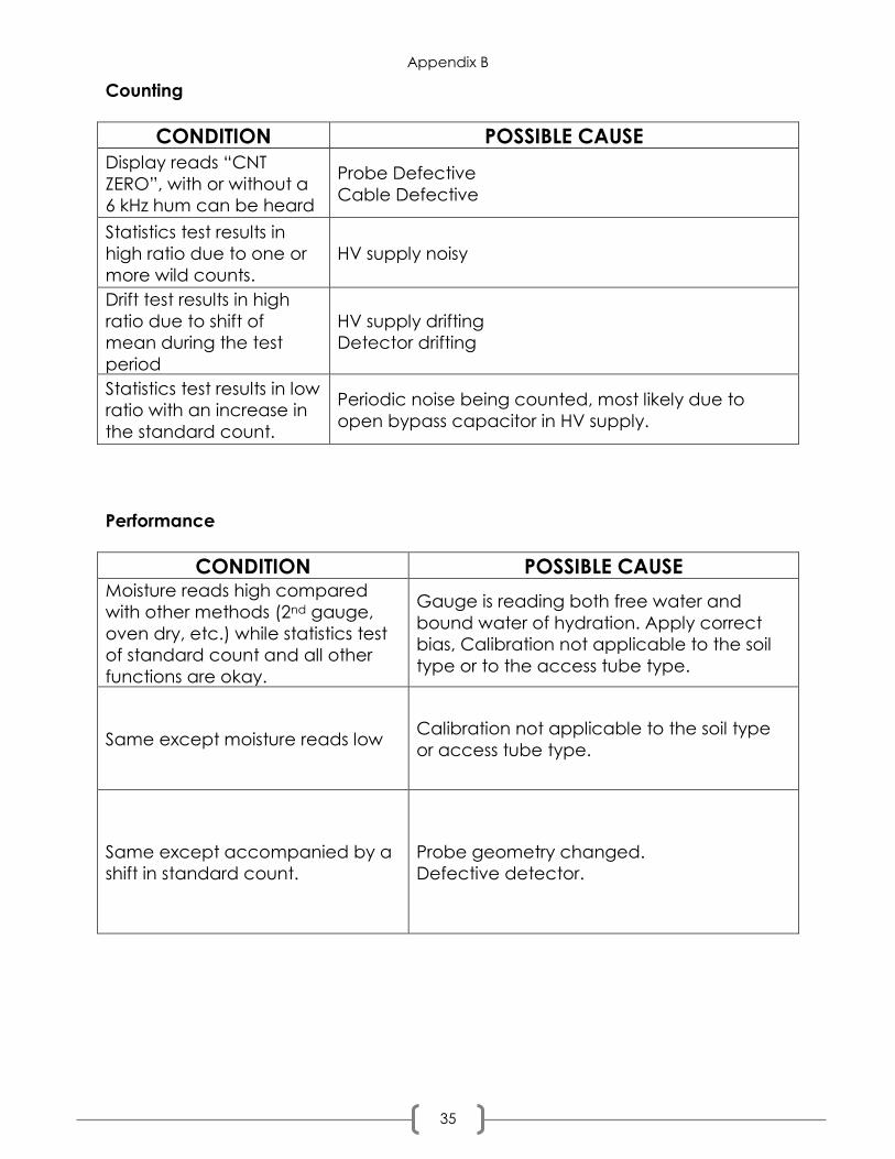
Counting

CONDITION POSSIBLE CAUSE

Display reads “CNT

ZERO”, with or without a

6 kHz hum can be heard

Probe Defective

Cable Defective

Statistics test results in

high ratio due to one or

more wild counts.

HV supply noisy

Drift test results in high

ratio due to shift of

mean during the test

period

HV supply drifting

Detector drifting

Statistics test results in low

ratio with an increase in

the standard count.

Periodic noise being counted, most likely due to

open bypass capacitor in HV supply.

Performance

CONDITION POSSIBLE CAUSE Moisture reads high compared

with other methods (2nd gauge,

oven dry, etc.) while statistics test

of standard count and all other

functions are okay.

Gauge is reading both free water and

bound water of hydration. Apply correct

bias, Calibration not applicable to the soil

type or to the access tube type.

Same except moisture reads low Calibration not applicable to the soil type

or access tube type.

Same except accompanied by a

shift in standard count.

Probe geometry changed.

Defective detector.

Appendix C

36

Appendix C

Print/Data Transfer Using the logging feature, the gauge can record many records of site readings

for recall later. It is extremely convenient if that data can be used in a program

that can manipulate the data for the user needs. To get the data from the

probe to the computer

To download project data:

Press MENU – Use Arrow keys to select 4. Projects.

Press ENTER – Use Arrow keys to select 4. Save Projects

Press ENTER – Select:

1. Send Project to USB – Project will be saved on Thumb drive in .XLS format.

2. Send All to USB – All projects will be saved on Thumb drive in .XLS format.

3. Send Project Serial – Project will be sent to PC over a RS232 connection

4. Send All Serial – All projects will be sent to PC over a RS232 connection

5. Legacy Format – CPN DR Dump Software.

The program specifications that pertain to the gauge are:

RS232 type serial communication (TXD, RSD, GND)

I start bit, 8 data bits, no parity, and 1 stop bits.

Baud rate: 115200

503 Hydroprobe Control Software

The program connects to the 503

through a USB serial cable from the

pc to the gauge. It permits the user

to control the gauge from the pc,

download data from the gauge, and

upload calibrations and templates to

the gauge.

Downloaded data can be saved as

XLS, CVS, or text file.

Appendix D

37

Appendix D

Counting Statistics

General

Radioactive decay is a random process. For Cesium-137, which has a half-life of

30 years, it can be expected that in 30 years one-half of the material will have

decayed, but in the next minute exactly which atoms will decay and exactly

how many will decay is only by chance. Repeated measurements with the

gauge will thus most likely result in a different count for each measurement. A

typical set of 32 such measurements is shown in Figure D.1.

Fig. D.2 shows the distribution of these counts. The

two characteristics of interest are: 1) the average

value (also called measure of central tendency or

mean), and 2) how wide the counts spread around

this average.

Mathematically the average value is defined as:

n

xx

The width of the spread is defined by a term called

standard deviation.

1

)( 2

n

xxs

Or an alternate form useful on calculators:

1

22

nn

ns xx

where:

s = standard deviation of the sample

x = count (value of each sample)

x = average of the sample

n = number of measurements in the sample.

The above describes the average value and the

standard deviation of a sample from a population.

They are in approximation to the true average value

and true standard deviation of the population.

μ = true average of the population

σ = true standard deviation of the population

SAMPLE COUNT

32 4370

31 4370

30 3742

29 4370

28 4370

27 3812

26 4370

25 4370

24 4402

23 4370

22 4370

21 4370

20 3636

19 4370

18 4370

17 3566

16 4370

15 4370

14 4370

13 4368

12 4370

11 4368

10 4370

9 3730

8 4368

7 4370

6 4370

5 4370

4 4370

3 4370

2 4370

1 4370

Figure D.1

Appendix D

38

Figure D.2

Figure D.3 Figure D.4

The distribution from measurement samples of any

process can be classified into expected shapes

that have been previously observed. Three are

applicable to radioactive decay; Binomial, Poisson

and Normal (also called Gaussian).

The Binomial distribution applies when the

measured event can take one of two states.

Tossing a coin is an obvious case. It can also be

applied to a given atom, either decaying or not, in

a time period. It is difficult to deal with

computationally.

Since the number of atoms is very large and the

expected probability of a decay occurring is very

low (source life in years and measurement time in minutes), we can use the

Poisson distribution which is a special case of the binomial distribution for these

conditions. A special property of the Poisson distribution is that the expected

standard deviation is equal to the square-root of the average value.

x

If the sample is large enough, we can approximate for the standard deviation of

the sample.

This is an important relationship. It means that if repeated measurements are

taken without moving the gauge and the detector electronics are working

properly, then the spread of the counts will only be dependent upon the

average count rate. This is in contrast to most measurements where the spread

will depend upon the process. Figure D.3 shows the diameter of a part turned on

a new lathe while

Figure E.4 shows the

same part turned on a

old lathe. Both lathes

produce a part with

the same average

diameter but a loose

bearing caused the

wider spread for parts

manufactured on the

older lathe.

Appendix D

39

The Poisson distribution to discrete measurements, e.g. count or not count.

Provided the average value is large enough (20 or greater), the Poisson

distributions can be approximated by the Normal distribution.

Using the Normal distribution simplifies things even further. It is a continuous

distribution. It is symmetrical about the average, and most important, it can be

completely described by its average and standard deviation.

As shown in Figure D.5., for a normal distribution, 68.3% of all counts will be within one

standard deviation, 95.5% of all counts will be within

two standard deviations, and 99.7% of all counts will

be within three standard deviations.

Thus, these three distribution models become

identical for the case with a small individual success

probability, but with a large number of trials, so that

the expected average number of successes is large.

This allows the use of the best features of each

distribution for three statistical situations concerning

the gauge:

1) Single measurement precision.

2) Expected spread of measurements.

3) Expected difference between two measurements.

Figure D.5

Appendix D

40

Single Measurement Precision

The expected variation for one standard deviation (68.3%) of a single count can

be expressed as a percent error as follow:

%ERROR = 100 xx

x 1100

This expression reveals that the only way to improve the count precision (e.g.

reduce the percent error) is to increase the size of x (e.g. the gauge

manufacturer selects components for a higher count rate while gauge user

counts for a longer period of time).

The following table demonstrates that a minimum of 10000 counts of readings is

required to achieve a count precision of 1.0 percent or better, 68.3% of the time.

Counts Square Root Count Precision

(68.35)

Count Precision

(95.5%) 1 1.00 100.00

10 3.16 31.60 63.2

100 10.00 10.00 20.0

1000 31.62 3.16 6.32

10000 100.00 1.00 2.00

100000 316.22 0.32 0.63

The count precision improves with the square of the count. Thus taking four times

the counts improves the count precision by a factor of two.

To provide a consistent frame of reference to the operator, the count displayed

in the DR is always an equivalent to 60-seconds count or CPM (counts per

minute), regardless of the time base selected. It is necessary to correct a

precision determination for other time base selections as follow:

%ERROR

60

1100

tx

Where t is the selected time in seconds.

Example:

A 60-second direct count is taken and displays 3000. The precision of the

count is:

Appendix D

41

Precision %82.1

60

60.3000

100

The direct reading is 2.0 gm/cm³. To determine the end measurement precision,

it is a necessary to multiply the count precision by the slope of the calibration

curve. Assuming a slope of 0.0416 gm/cm³ per percent, the 2.0 gm/cm³

reading varies by +/- 0.076 gm/cm³ (68% of the time representing one standard

deviation).

If you take repeat measurements but move the gauge between readings, then

the standard deviation of that set of readings will include both the source

random variation and the variation due to re-positioning the gauge, and thus

be larger.

Expected Spread of Measurements

An accepted quality control procedure for a random counting device is to

record a series of 20 to 50 successive counts while keeping all conditions as

constant as possible. By comparing the distribution of this sample of counts with

the expected Normal distributions, abnormal amounts of fluctuation can be

detected which could indicate malfunctioning of the gauge.

The “Chi-squared test” is a quantitative means to make this comparison. It can

be used when a calculator is available to determine the standard deviation of

the sample.

2

22 )1(

sn

where 2 is from the Chi-squared tables.

By substituting the expected standard deviation with the square-root of the

average count

x ; re-arranging terms and taking the square-root of both

sides, we obtain:

x

s

n

1

2

Ideally the ratio on the right hand side of this expression should be 1.00. The

degree to which this ratio departs from unity is indicator of the extent to which

the measured standard deviation differs from the expected standard deviation.

Appendix D

42

On the left hand side of the expression, the degree to which 2 differs from (n-1)

is a corresponding allowance for the departure of the data from the predicted

distribution (e.g. we flip a coin ten times and expect five heads and five tails, but

accept other distributions for a given sample). Chi-squared distribution tables

are found in texts on statistics. The table values depend upon the degrees of

freedom (one less than the number of counts) and the probability that a sample

of counts would have a larger value of 2 than in the table. The 2 values for

2.5% and 97.5% (a 95% probability range) and 31 degrees of freedom are 17.54

and 48.23. Substituting these values into the left hand side of the expression

gives ratio limits between 0.75 and 1.25 for 32 samples and a 95% probability.

If the ratio on the right side is between these limits, then there is no reason to

suspect the gauge is not performing properly. If the ration is outside these limits,

then the gauge is suspect and further tests are in order (even a properly working

gauge will fall outside of the Chi-squared limits 5% of the time).

If a calculator is not available which can easily determine the standard

deviation, a qualitative method to compare the observed standard deviation

with the expected standard deviation is to take a series of 10 counts and

determine their mean and the square-root of their mean (guess the square-root

to 2 digits if not available on the simple calculator). If their distribution is normal,

then 68.3% of the readings will be within the mean +/- the square-root of the

mean (e.g. 7out of 10).

Expected difference between two readings

The standard count or some other reference count should be recorded on a

regular basis to allow observing if it stays the same or if any adverse trends are

present. If enough counts have been used to determine the average, and also

the standard deviation of the population, then the Normal distribution may be

used.

n

xz

Expressing the x value in them of the value plus a factor of the deviation:

nkZ

kx

From the Normal tables, for 95% confidence, the Z value is 1.96.

Appendix D

43

96.11

196.

n

ZK

Thus the new reading should be equal to the average of the old reading

plus/minus 1.96 times the square-root of the old average.

This is true for the 60-second count which is direct. For another time base, the K

term must be reduced by the square-root of the count pre-scaling (e.g. for a

240-second count which is 4 times as long as the direct 60-second count, the

new reading should be plus/minus 0.98):

98.0

4

96.1

n

ZK

This is the case when the standard count is taken which involves 240 each

(n=240/60=4) 1-second counts. A new standard count should be equal to the

old standard count plus/minus 0.98 times the square-root of the old standard

count 95 percent of the time.

EXAMPLE:

The average of the daily standard count for the last month is 10,000. The square-

root of this average is 100. A new standard count (240 each at 1 seconds, but

displayed as 60 seconds, CPM) should be between 9,902 and 10,098 with a 95%

of probability.

Index

44

Appendix E

Connectors Pinouts

The pinout of the MOLEX connector in the rear panel of the gauge is as follows:

Pin number Function

A Power + 10Vdc

B Not used

C Ground

D Detector Signal

Index

45

Appendix F

Sample of Data downloaded via the thumb drive to an Excel spread sheet.

Index

46

Appendix G

Access Tubing Almost any tube type can be used as long as the probe is calibrated with the

same type of tube that is used in the field. The ideal tubing has a minimum wall

thickness and is strong enough to prevent damage and bending during

installation. The tubing should be capped at the top and bottom if to prevent

water from getting inside.

Aluminum 6061-T6 This tubing is ideal for minimal moisture sensitivity.

It can be installed easily in rocky soils.

Thicker walled versions (.125”) won’t dent easily and will last longer.

Steel: Carbon and Stainless This is expensive but very durable in rocky soils.

Some larger wall thickness versions can be flush coupled and thread together.

Some measurement sensitivity.

PVC Schedule 125 This is inexpensive and readily available.

Sunlight may cause brittleness and cracking to exposed tubing.

The chloride content will reduce the response on the moisture measurement.

The factory calibrations determined on all new 503DR gauges are based on an

aluminum tubing calibration. This calibration can be adjusted to represent the

other tubing types listed here.

Index

47

Index

A Americium · 6

B Battery Life · 6

C Cable Stops · 7

Calibration · 23

Chi-squared · 34

Connectors Pinouts · 44

Controls and Display · 9

Count Time · 8

D Data Storage · 13

Data Transfer · 36

Dimensions · 5

E Encapsulation · 6

Error Messages · 33

F Features · 2

Field Calibration · 23

Functional Description · 3

G Getting Started · 8

H Humidity · 6

I Inspection · 7

L Laboratory Calibration · 24

Leak Testing · 30

Log · 13

M Maintenance · 29

N Neutron Source · 6

O Operation · 12

P Performance · 5

Precision · 5

Probe Assembly · 31

Production Description · 1

R Radiological · 6

Recall · 20

S Shielding · 6

Shipping Requirements · 6

Shipping Weights · 5

Special Form Approval · 6

Specifications · 5

Standard Count · 12, 21

Standard Equipment · 4

Surface Electronic Assembly · 31

T Taking A Reading · 12

Taking a Standard Count · 21

Temperature

Operating · 6

Storage · 6

TI · See Transport Index

Time · 10, 12

Transport Index · 6

Troubleshooting · 34

Tube Adapter Ring · 7

U Units · 10,12