Covid-19 Supply Chain Disruptions

Collaborative Research Center Transregio 224 - www.crctr224.de

Rheinische Friedrich-Wilhelms-Universität Bonn - Universität Mannheim

Discussion Paper No. 239 Project C 02

Covid-19 Supply Chain Disruptions

Matthias Meier 1 Eugenio Pinto 2

November 2020

1 University of Mannheim, Department of Economics, Block L7, 3-5, 68161 Mannheim, Germany; E-mail: [email protected]

2 Federal Reserve Board; E-mail: [email protected]

Funding by the Deutsche Forschungsgemeinschaft (DFG, German Research Foundation) through CRC TR 224 is gratefully acknowledged.

Discussion Paper Series – CRC TR 224

Covid-19 Supply Chain Disruptions∗

Matthias Meier† Eugenio Pinto‡

November 15, 2020

Abstract

We study the effects of international supply chain disruptions on real economicactivity and prices during the Covid-19 pandemic. We show that US sectors witha high exposure to intermediate goods imports from China contracted significantlyand robustly more than other sectors. In particular, highly exposed sectors sufferedlarger declines in production, employment, imports, and exports. Moreover, input andoutput prices moved up relative to other sectors, suggesting that real activity declinesin sectors with a high China exposure were not particularly driven by a slump indemand. Quantitatively, sectors at the third quartile of China exposures experiencedlarger monthly production declines of 2.5 p.p. in March and 9.4 p.p. in April 2020 thansectors at the first quartile. Differences in China exposures account for about 10% ofthe cross-sectoral variance of industrial production growth during March and April.The estimated effects are short-lived and dissipate by July 2020.

Keywords: Supply chain disruptions, Covid-19, industrial production.

∗We thank Harald Fadinger, Efi Adamopoulou, and participants in the Mannheim Internal Seminar foruseful comments. Matthias Meier gratefully acknowledges funding by the German Research Foundation(DFG) through CRC TR 224 (Project C02), and financial support from the UniCredit & Universities Foun-dation. The analysis and conclusions are those of the authors and do not indicate concurrence by the Boardof Governors of the Federal Reserve System or other members of its research staff. We thank Paul Tran forexcellent research assistance.

† Universität Mannheim, Department of Economics, Block L7, 3-5, 68161 Mannheim, Germany; E-mail:[email protected]

‡ Federal Reserve Board; E-mail: [email protected].

1

mailto:[email protected]

[email protected]

1 Introduction

Over the past decades, economies around the globe have become increasingly interconnectedthrough trade and global value chains. In this environment, disruptions to the flow ofgoods across borders can have large economic effects. In recent years, such disruptions havebeen occurring at an increasing frequency, as the US-China trade war, Brexit, and policyinterventions related to the Covid-19 pandemic suggest. In this paper, we study the effectsof supply chain disruptions on the US industrial sector during the Covid-19 crisis.

The Covid-19 crisis caused sharp contractions in economic activity across most sectorsand economies. For US industrial production, the rapid decline during March and April2020 dwarfs even the Great Recession (Figure 1). The Covid-19 crisis affected the economythrough a number of different channels. These include direct channels operating throughthe health of the population, mandated lockdowns, and disruptions to trade, as well asother more standard channels, such as downbeat consumer and business sentiment, highuncertainty, and financial stress. Understanding the role of these channels is importantfor an effective policy response. For example, lockdowns can disrupt supply chains acrosscountries and sectors. If production is suppressed because of disrupted supply chains, afiscal intervention to stimulate demand may be ineffective. Conversely, providing liquidityor flexible furlough arrangements may be a more effective policy response to facilitate a quickrecovery when the supply chain disruption dissipates.1

When the US-China trade deal was signed in January 2020, this was positive news for USsectors highly dependent on imports from China. Not long after, however, China respondedto the emerging Covid-19 pandemic by imposing widespread lockdowns of entire regionsand sectors during February and part of March 2020. In China, the lockdowns causedsharp contractions in production and exports, which eventually spilled over to the US. Infact, US imports from China declined, but mostly in March rather than in February (afteraccounting for seasonality and calendar effects including the Chinese New Year). The slightdelay between the February lockdowns in China and the observed decline in US importsfrom China likely reflects transit time. Moreover, the decline in imports from China wasespecially large for intermediate goods, resulting in major supply chain disruptions for USproducers.

We study the effects of disruptions to supply chains connected to China on US real

1An early discussion of the implications for policy of the Covid-19 crisis is provided by Baldwin anddi Mauro (2020). By now, an extensive literature studies the policy implications of Covid-19: On optimallockdown policy, see, e.g., Alvarez et al. (2020), Eichenbaum et al. (2020), Krueger et al. (2020), and Gloveret al. (2020); on the effects of fiscal policy, see, e.g., Bigio et al. (2020), Mitman and Rabinovich (2020),Auerbach et al. (2020), and Bayer et al. (2020); and on monetary policy, see, e.g., Caballero and Simsek(2020), Woodford (2020), and Fornaro and Wolf (2020).

2

Figure 1: Aggregate US industrial production

2020m3

2020m4

-4.30

-12.81

-15

-10

-50

5

2005m1 2010m1 2015m1 2020m1

Monthly %-change in industrial production

Notes: The time series is the monthly percentage change in industrial production(seasonally adjusted), based on the Federal Reserve G.17 release. Recent monthsstarting from February 2020 are highlighted by an ‘x’. The growth rates for March andApril are printed into the plot. Gray-shaded areas indicate NBER recession periods.

economic activity and prices during the Covid-19 crisis on a monthly basis. Our empiricalstrategy exploits variation in the share of imported intermediate goods across sectors beforeCovid-19.2 The simple idea is that sectors that are more dependent on inputs imported fromChina should also be more affected by supply chain disruptions stemming from the initialCovid-19 crisis in China.

We show that US sectors with high exposure to Chinese imports contracted significantlyand robustly more than other sectors. In particular during March and April 2020, highlyexposed sectors suffered larger declines in production, employment, imports, and exports.Quantitatively, sectors at the third quartile of China exposures experienced larger monthlyproduction declines of 2.5 percentage points (p.p.) in March and 9.4 p.p. in April comparedto sectors at the first quartile. Differences in China exposures account for about 10% of thecross-sectoral variance of industrial production growth during March and April. These differ-ential effects appear to be relatively short-lived and become insignificant by July. While ouranalysis focuses on Covid-19 disruptions of US-China trade, we also consider a broader andcomplementary exposure to intermediate good imports, which includes all imports exceptfrom China, and, thus, is referred to as ex-China exposure. Sectors with a high ex-Chinaexposure to imported inputs also suffer larger output declines, but the response of employ-

2Using sectoral data in our analysis has some important advantages compared to using firm-level data.In particular, we can use monthly data that are publicly and quickly available in real time. For example,monthly sectoral industrial production is released two weeks after the end of the month.

3

ment and export is insignificant.A critical question is whether our exposure measure captures the strength of supply-

chain shocks across US sectors. Instead, our exposure measure might be high for industriesthat were also more affected through other channels during the Covid-19 recession, suchas a slump in domestic demand, weaker external demand (namely from China), or tighterfinancing conditions. We address this concern in two ways. First, we control for sector-specific cyclicality, for exports to China, and for external finance dependence, all beforeCovid-19. Including these controls, we still find a significant relation between a higherChina exposure and a larger contraction in industrial production. Second, we estimate howhigher China exposure relates to sectoral prices. We find that both input import prices andoutput prices increase by significantly more for sectors with higher China exposure. Thisresult makes it unlikely that changes in real activity in industries with high China exposurewere mostly affected by lower domestic or external demand. In contrast, industries with alarger share of the ex-China imported intermediates experienced smaller input import andoutput price changes relative to other industries. This finding suggests that the broaderex-China exposure captures mostly the effects of lower demand across sectors.

To construct sector-specific exposure measures, we combine detailed 6-digit NAICS importdata for 2019 from the US Census with benchmark 6-digit input-output (IO) tables for 2012from the US Bureau of Economic Analysis (BEA). We aggregate these data to compute expo-sure measures for 88 manufacturing and related industries (approximately 4-digit NAICSlevel), which we can match to the level of sector detail available in the monthly industrialoutput and other data. For the China exposure, we construct the sector-specific value ofintermediate goods imports from China and divide by the value of all intermediate goods usedby that sector. For the broad ex-China import exposure measure, we replace the numeratorby intermediate goods imports excluding Chinese imports. Our empirical approach studiesto what extent sector-specific ex-ante exposures can account for ex-post outcomes duringthe Covid-19 crisis. This approach can be justified by a simple model in which the share ofestablishments that use inputs imported from a specific country differs exogenously acrosssectors. We show that this model explains a monotonic relation between higher ex-anteexposures and larger ex-post output responses.

Despite the quickly growing empirical literature on the Covid-19 crisis, our paper isthe first to provide evidence on the effects of international supply chain disruptions causedby Covid-19.3 Our empirical results suggest significant albeit relatively short-lived effects

3Chetty et al. (2020) document that lower spending of high-income individuals led to job losses for low-income individuals. Bachas et al. (2020) document a large increase in liquid asset savings across the incomedistribution. Balleer et al. (2020) use firm-level price data to disentangle demand and supply effects, whereasBrinca et al. (2020) disentangle labor supply and demand effects of the Covid-19 crisis.

4

of Covid-19 supply chain disruptions. The evidence is not only important for the designof effective macroeconomic stabilization policy, it also relates to questions on the natureof the business cycle. For example, the Great Moderation is often associated with lowervolatility in inventory investment (McConnell and Perez-Quiros, 2000), which can be linkedto innovations in just-in-time inventory management (Kahn et al., 2002). While lean supplychains reduce inventory holding costs and raise productivity in normal times, they can alsolead to more severe effects from downturns featuring disruptions to supply chains. Indeed,the impact of the Covid-19 crisis on supply chains and how to make them more resilienthave received a lot of attention starting from March 2020. These include the managementliterature, business consultancies, but also the media reporting on supply chain issues relatedto widespread lockdowns in China (see, for example, Choi et al., 2020, Schmalz, 2020, andDonnan et al., 2020). The Covid-19 crisis might even be a turning point for de-globalization(Antràs, 2020).

Closely related are a number of papers that analyze the propagation of Covid-19 relatedshocks through input and output linkages. For example, Barrot et al. (2020) study theeffects of social distancing on GDP, Baqaee and Farhi (2020) study the role of demand andsupply shocks during the Covid-19 crisis, and Bonadio et al. (2020) study the internationalpropagation of labor supply shocks. Closely related is also Gerschel et al. (2020), whosimulate the effect of a productivity decrease in China on GDP outside China. GDP in theUS responds similarly to France and Germany, whereas GDP in Japan and Korea respondsmuch more, reflecting the higher exposure of these economies to inputs imported from China.

Our paper is further related to earlier work on supply chain disruptions including Barrotand Sauvagnat (2016) and Meier (2020) on natural disasters in the US, Carvalho et al.(2020) and Boehm et al. (2019) on the Fukushima disaster, and Glick and Taylor (2010)on trade disruptions caused by war. The empirical strategy our paper uses is similar toBoehm et al. (2019), as well as Huang et al. (2018), Flaaen and Pierce (2019), and Amitiet al. (2020), who study the US-China Trade War. Our empirical findings align well withthe findings in Hassan et al. (2020). Analyzing earnings calls by public listed firms in thefirst quarter of 2020, the authors document that firms’ primary concerns are the collapseof demand, increased uncertainty, and disruption in supply chains. Interestingly, firms withprior pandemic experience (SARS or H1N1) are more resilient to the Covid-19 crisis.

The remainder of this paper is organized as follows. Section 2 presents a simple modelto provide intuition and to guide the empirical analysis. Section 3 describes the data andSection 4 presents our empirical findings. Section 5 concludes and an Appendix follows.

5

2 A simple model of supply chain disruptions

Consider a sector in country A that is populated by two types of establishments. Type 1establishments produce goods y1

t using imported intermediate goods from country B, denotedm1

t , and a range of other inputs, such as capital, labor, and other imported or domesticintermediate inputs, captured by a composite factor x1

t . The production technology is of theCES type

y1t =

[α(x1

t )ρ + (1 − α)(m1t )ρ

] 1ρ = f(z1

t )m1t , z1

t = x1t

m1t

, ρ ∈ (−∞, 1),

where σ = 1/(1−ρ) is the substitution elasticity between x1t and m1

t and z1t is the ratio of the

composite factor to country B intermediate inputs (factor input ratio). Type 2 establishmentsproduce goods y2

t using a linear technology in x2t . Hence, they use the same inputs as type

1 establishments except imported intermediate goods from country B. Sectoral output is

yt = ϕy1t + (1 − ϕ)y2

t , (2.1)

where ϕ is the (sector-specific) share of type 1 establishments. Before the economy is hit bya supply-chain disruption shock, it is in steady state and type 1 establishments choose x1

and m1 to maximize period profits

π1 = p(y1)y1 − pxx1 − pmm1, (2.2)

where p(y) = yγ−1 with γ ∈ (0, 1) is a downward-sloping isoelastic inverse demand function.Similarly, type 2 establishments choose x2 to maximize π2 = p(y2)y2 − pxx2. Since only type1 establishments use mt, we will henceforth omit the type index of m1

t and z1t .

In period t, the economy is hit by a supply chain disruption that lowers the supply ofcountry B inputs by a fraction δ for all sectors in the economy: mt = (1−δ)m.4 We considerthe response of type 1 establishments before prices adjust. The supply of mt becomes abinding constraint, which means type 1 establishments only re-optimize x1

t after the disrup-tion. The first-order condition for x1

t after the supply chain disruption implies that the factorinput ratio zt is adjusted according to (see Appendix A)

d log zt

d log mt

= − 1 − γ

(1 − ρ) − (γ − ρ)ϵ≤ 0, where ϵ = zf ′(z)

f(z)≥ 0. (2.3)

4A supply chain disruption that is common across sectors should capture the disruptions caused by thewidespread lockdowns in China during February and March 2020.

6

The increase in zt in response to a decrease in mt gets smaller the lower the elasticityof substitution between the two inputs to production. For example, in the Leontieff case(ρ → −∞), if mt falls by δ%, it is optimal to lower x1

t by δ% as well, and hence zt remainsunchanged. The effect on output y1

t depends on the direct effect of lower mt and a (partially)offsetting indirect effect of higher zt,

d log y1t = d log mt︸︷︷︸

direct effect< 0

+ −(1 − γ)ϵ(1 − ρ) − (γ − ρ)ϵ

d log mt︸︷︷︸indirect effect≥ 0

. (2.4)

The percent decline of output can vary between no response (perfect substitutes, ρ = 1),and a percent decline of output equal the percent decline of inputs (perfect complements,ρ → −∞). The response of sectoral output to the supply chain disruption is

d log yt = ϕy1

ϕy1 + (1 − ϕ)y2(1 − ρ) − (1 − ρ)ϵ(1 − ρ) − (γ − ρ)ϵ

d log mt. (2.5)

If γ → 1 or ρ → −∞, the response of sectoral output only depends on the output share oftype 1 establishments.

Our empirical strategy is to identify cross-sector differences in effects of supply chaindisruptions through cross-sector differences in the share of intermediate goods importedfrom country B. In the model, import exposure to country B is

eB = pmm

px(x1 + x2) + pmm, (2.6)

and eB monotonically increases in ϕ. Simultaneously, the sector-specific output responseto a supply-chain disruption monotonically increases in ϕ, the share of establishments thatproduce using imports from country B. Hence, sectors with a higher import exposure alsorespond more to a common supply chain disruption. This provides justification to ourempirical strategy.

Finally, we discuss the robustness of these results. First, if we fix ϕ but let α varyacross sectors, we obtain similar results as long as inputs in type 1 production are somewhatsubstitutable (ρ > −∞). The sector with a lower α has a higher expenditure share eB form. At the same time, a lower α implies a lower elasticity ϵ, which results in a larger outputresponse to the supply chain disruption. Second, our analysis has conveniently maintainedfixed input prices. If prices for the same inputs are common across sectors, the specificresponse of prices to the shock does not qualitatively change our result that in sectors withhigher exposure to imported intermediate goods output should fall by relatively more.

7

3 Data

3.1 Covid-19 and imports from China

In response to the Covid-19 outbreak, China imposed widespread lockdowns of entire regionsand sectors during February and part of March 2020. In the aftermath of these disruptions,US imports from China plummeted in March (Figure 2), after accounting for seasonalityand calendar effects (including the Chinese New Year).5 The decline was more noticeablefor intermediate goods imports from China, which rebounded well above the pre-crisis levelonce the effects of lockdowns in China dissipated. This suggests that US producers weresubject to a major supply chain disruption. In addition, imports of intermediate goods fromall other countries (ex-China) did not increase during February and March, which suggestslow short-run substitutability of the disrupted supply from China. In fact, imports ex-Chinaonly start falling by April, and more severely so for final goods. This seems consistent withex-China imports being driven by lower demand during the Covid-19 crisis in the US.

3.2 Outputs, inputs, and prices

We consider a host of sector-level outcomes including measures of output, inputs, and prices.Industrial production (IP) is our primary outcome. IP is a monthly index computed fordetailed (usually 4- to 6-digit NAICS) manufacturing sectors by the Federal Reserve Board,and is constructed from an extensive range of data. For about 50% of industries, the index isbased on observed physical quantities. For example, for NAICS sector 3361 (Motor vehicle)IP is based on the number of types of automobiles produced together with their list pricesobtained from Ward’s Communications, a publisher focused on the automotive industry,and car producers Chrysler and General Motors.6 For the remaining 50% of industries,the Federal Reserve Board combines production-worker hours from the Bureau of LaborStatistics (BLS) and Fed data on electric power use with product prices from the BLSand spot markets to construct an industry-specific index of IP. The indexes are regularlybenchmarked against the Economic Census and the Annual Survey of Manufacturers.

5We separately construct US imports of intermediate and final goods based on the methodology describedin Section 3.3. We seasonally adjust the aggregate data using X-13ARIMA-SEATS. We account for calendareffects due to trading days and Easter and allow for automatic outlier detection. For imports from China, wealso account for Chinese New Year calendar effects in a way similar to Roberts and White (2015): we followthe People’s Bank of China and assume fixed sub-period lengths of 20, 7, and 20 days around the ChineseNew Year (plus 3-weeks to account for transportation transit time). We use the data from 2010-2019 toestimate the seasonal and calendar effects, including the Chinese New Year, in 2020.

6More details on the data sources for the construction of the industrial production index can be foundhere: https://www.federalreserve.gov/releases/g17/SandDesc/sdtab1.pdf

8

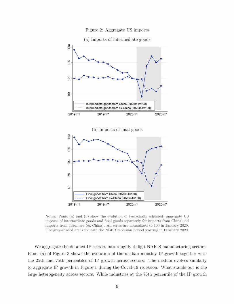
https://www.federalreserve.gov/releases/g17/SandDesc/sdtab1.pdf

Figure 2: Aggregate US imports

(a) Imports of intermediate goods

8010

012

014

0

2019m1 2019m7 2020m1 2020m7

Intermediate goods from China (2020m1=100)Intermediate goods from ex-China (2020m1=100)

(b) Imports of final goods

6080

100

120

140

2019m1 2019m7 2020m1 2020m7

Final goods from China (2020m1=100)Final goods from ex-China (2020m1=100)

Notes: Panel (a) and (b) show the evolution of (seasonally adjusted) aggregate USimports of intermediate goods and final goods separately for imports from China andimports from elsewhere (ex-China). All series are normalized to 100 in January 2020.The gray-shaded areas indicate the NBER recession period starting in February 2020.

We aggregate the detailed IP sectors into roughly 4-digit NAICS manufacturing sectors.Panel (a) of Figure 3 shows the evolution of the median monthly IP growth together withthe 25th and 75th percentiles of IP growth across sectors. The median evolves similarlyto aggregate IP growth in Figure 1 during the Covid-19 recession. What stands out is thelarge heterogeneity across sectors. While industries at the 75th percentile of the IP growth

9

distribution shrank by around 5% in April 2020, industries at the 25th percentile shrank bymore than 20%. Growth rates of IP and other variables, xt, in this paper are symmetricgrowth rates of the form

xt − xt−h12 (xt + xt−h)

, (3.1)

where t is a monthly time index, h = 1 for monthly growth rates, and h = 12 for yearly (12-month) growth rates. At least since Davis and Haltiwanger (1990) these growth rates havebeen widely used to study establishment-level employment growth. Symmetric growth rateslie in the closed interval [−2, 2] and avoid extreme statistical outliers when some outcomedrops close to zero. This concern is specifically prevalent during the sharp contractions ofthe Covid-19 recession.7 However, our results are robust to using standard growth rates.

We further use sector-specific employment, imports, exports, import prices and outputprices. We obtain employment from the Current Employment Statistics maintained by theBLS. Sector-specific imports and exports are from the International Trade Data maintainedby the Census Bureau. We construct sector-specific prices for intermediate inputs importsby combining product-specific price indexes from the BLS International Price Index fileswith the sector-specific composition of intermediate inputs imports from the BEA importmatrix. Output prices are based on the sector-specific producer price indexes maintained bythe BLS. In addition, we construct a number of control variables. We consider a measure ofsectoral external finance dependence following the approach in Rajan and Zingales (1998),but using data between 2010 and 2019. We use sector-specific exports to China based onthe International Trade Data. Finally, we consider a measure of sectoral cyclicality, whichwe compute as the correlation between sectoral annual IP growth and annual (aggregate)GDP growth, based on data before the Covid-19 crisis.

3.3 China exposure

We compute the sector-specific China exposure as the value of imported intermediate goodsfrom China relative to the value of all intermediate goods used in production. However,sector-specific intermediate good imports from China are not directly measured by tradestatistics. Instead, we observe imports from China in 2019 at the level of 6-digit NAICScommodities from the International Trade Data. In addition, we have the value of 6-digitNAICS commodity imports (from all countries) used by 6-digit NAICS sectors from the

7For example, the (ordinary) monthly growth rate of IP in sector 3361 (Motor Vehicle Manufacturing) isbelow -97% in April 2020 compared to March, and above +1,000% between April and May. For comparison,the symmetric growth rates in sector 3361 for April and May are -190% and +170%, respectively.

10

Figure 3: Heterogeneity across sectors

(a) Distribution of industrial production growth across sectors

-30

-20

-10

010

2019m1 2019m7 2020m1 2020m7

Median of IP growth25th and 75th percentiles

Monthly %-change in sectoral IP

(b) Distribution of Chinese exposure across US sectors

05

1015

2025

Num

ber o

f sec

tors

0 1 2 3 4 5%-share of China imported intermediate inputs

Notes: Panel (a) shows the three quartiles of monthly percentage change in industrialproduction (seasonally adjusted), based on the Federal Reserve G.17 release. The gray-shaded area indicates the NBER recession period starting in February 2020. Panel (b)shows the histogram of China exposures across US sectors.

import matrix of the Bureau of Economic Analysis (BEA) 2012 Input-Output tables. Toconstruct sector-specific intermediate good imports from China, we adopt a proportionalityassumption, as described in Johnson and Noguera (2012) and as similarly applied to constructthe World Input Output Database (see Timmer et al., 2015). In practice, we proceed in threesteps to compute sector-specific intermediate good imports from China. First, we compute

11

the share of 6-digit NAICS commodities that is imported from China relative to all importsof the same commodity. Second, we multiply the value of a 6-digit sector’s 6-digit commodityimports (from all countries) with the China import share of the 6-digit commodity. Thisyields an estimate of the value of imports from China of 6-digit commodities in 6-digitsectors, which is exact under the proportionality assumption. Third, we aggregate acrossall 6-digit commodities to obtain the total value of intermediate goods imports from Chinafor each 6-digit sector. We obtain the value of all intermediate goods used in production foreach 6-digit sector from the input-output table. Our (baseline) China exposure is the ratioof intermediate goods imported from China divided by all intermediate goods, where boththe numerator and denominator are appropriately aggregated across the 6-digit sectors tothe roughly 4-digit NAICS sectors available for IP and other outcomes.

The final sample contains 88 distinct manufacturing and related industries. In theAppendix, Table 7 lists all industries. Panel (b) of Figure 3 shows the variation in Chinaexposures across these industries. We observe large differences in the share of intermediatesimported from China ranging from less than 0.25% to more than 2%. Throughout the empir-ical analysis, we discard sector 3342 (Communications Equipment Manufacturing), which isthe single outlier in the distribution of China exposures with a value close to 5%, see panel(b). While these fractions are relatively small, in theory a disruption in the supply of Chineseinputs can lead to as much as a complete halt of production in the US. The magnitude of theeffect critically depends on how easily inputs can be substituted (as implied by the simplemodel in the preceding section).

4 Empirical evidence

In this section, we provide empirical evidence suggesting that supply chain disruptions area significant economic driver of the Covid-19 crisis.

4.1 Empirical strategy

Our empirical strategy exploits differences in the sector-specific exposure to intermediatedgoods imported from some country or region, say B. Let i index a sector and t a monthlytime period. Our main regression model is

yit = αt + βteBi + ΓtZit + uit, uit ∼ (0, σ2

t ) (4.1)

where yit is a sector-time specific outcome expressed in growth rates (e.g., IP growth of steelmanufacturing in March 2020) and Zit is a vector of sector-time specific controls. Using the

12

notation of Section 2, we denote by eBi the import exposure to country/region B, which we

compute based on pre-Covid-19 data.Most of our empirical analysis focuses on China exposures (B = China). If the exposure

eChinai is orthogonal to channels other than supply chain disruptions that explain differential

outcomes across sectors, then βt will capture the causal effect of supply chain disruptions.Similar strategies have been employed by Boehm et al. (2019) in the context of the 2011Tohoku Earthquake, and in Huang et al. (2018), Flaaen and Pierce (2019), and Amiti et al.(2020) in the context of the US-China Trade War.

We next study whether industrial production fell by relatively more in sectors with higherChina exposure. This naturally raises endogeneity concerns, which we address in Section 4.3.In particular, we address the concern that βt may capture differential demand effects, bystudying the effects both on (output and input) quantities and on (output and input) prices.

4.2 Industrial production and China exposure

We first estimate the βt coefficients using a regression (4.1) of IP growth (yit) on Chinaexposure (eChina

i ) without controls (no Zit). Figure 4 shows the estimated βt coefficients overtime. The coefficients for March, April, and May 2020 stand out both in significance andmagnitude compared to the coefficients estimated over the preceding three years.

In fact, before the Covid-19 crisis, the βt coefficients are consistently close to zero andstatistically indistinguishable from zero. This may appear surprising against the backdropof the US-China trade war during these years. We propose two explanations. First, thetariffs imposed during the trade war often targeted specific sectors, e.g., washing machinesas analyzed in Flaaen et al. (2020). Our exposure measure is unlikely to pick up theseeffects. Second, while tariffs change the costs of imported inputs they do no prohibit goodsfrom being produced and transported across borders. In the short-run, higher tariffs haveplausibly weaker effects on production than lockdowns.

For February 2020, the positive coefficient may appear surprising at first glance. In fact,the Chinese New Year holidays were extended into the first weeks of February in many ofthe largest Chinese provinces, so we might expect a large negative coefficient already inFebruary. Three explanations can plausibly account for the non-negative βt. First, cargotransportation from a supplier in China to a US producer takes time.8 Second, US producershold some inventory of imports from China, which dampens the immediate effect. Third, theUS-China trade deal signed in January 2020 may have given a small boost to sectors withhigher China exposure. Relatedly, it may appear surprising that the βt coefficient peaks only

8Cargo ships travel 12 days from China to US West Coast and 22 days to US East Coast, see https://www.langsamreisen.de/en which offers freighter travel.

13

https://www.langsamreisen.de/en

https://www.langsamreisen.de/en

in April, whereas the main Chinese lockdown was in February. Apart from transportationtime and inventories, this may be explained by sustained (partial) lockdowns and restrictionson production in China. A further explanation is supply chain propagation within US sectors.For example, if only some firms are directly affected by the shock, the shock may only slowlyspread to other firms in the sector.

The main take-away from Figure 4 are the large βt coefficients in March and April 2020.The estimates are of economically relevant magnitudes. Industrial production growth isestimated to have been 3.8 percentage points (p.p.) and 14.2 p.p. lower in March and April,respectively, for every 1 p.p. increase in the China exposure across sectors (see first columnsin Table 1). The 25th percentile of China exposure across sectors is 0.33% while the 75thpercentile is 0.99%. Hence, sectors at the third quartile of China exposures experienced largermonthly production declines of about 2.5 p.p. in March and 9.4 p.p. in April than sectorsat the first quartile. To understand how much variation in IP growth can be explained byvariation in China exposures, note that the cross-sectional standard deviation of our Chinaexposure measure is σ(echina

i ) = 0.51%, and the standard deviations of IP growth in Marchand April 2020 are σ(yi,2020m3) = 7.20% and σ(yi,2020m4) = 24.79%. Hence, in terms of R-squared, 7.4 percent of the cross-sectoral variance in March IP growth and 8.6 percent inApril can be associated to different China exposures. To gauge the combined March and

Figure 4: Coefficient βt in a regression of IP on China exposure

2020m3

2020m4

-20

-10

010

20

estim

ated

coe

ffici

ent

2017m1 2018m1 2019m1 2020m1

Notes: Markers indicate the estimated coefficients βt in a regression of monthly IP growthin period t on China exposures according to (4.1). Vertical lines indicate 95% confidenceintervals.

14

Table 1: Industrial Production and China exposure

(a) IP growth in March 2020

Monthly Monthly/Detr. Yearly Yearly/Detr.China exposure -3.816 -3.740 -4.083 -2.875

(1.467) (1.451) (1.870) (1.831)Observations 87 87 87 87R2 0.074 0.072 0.053 0.028

(b) IP growth in April 2020

Monthly Monthly/Detr. Yearly Yearly/Detr.China exposure -14.23 -14.15 -16.25 -15.04

(5.016) (5.012) (5.669) (5.582)Observations 87 87 87 87R2 0.086 0.086 0.088 0.079Note: Based on regression (4.1). Standard errors in parentheses. The pointestimates in the first column of panels (a) and (b) are identical to the March andApril 2020 coefficients in Figure 4.

April effect of China exposure on industrial production, we use the year-over-year IP growthin April 2020 as outcome variable (see third column of panel (b) in Table 1). We concludethat 8.8 percent of the variance in industrial production during the Covid-19 crisis can beattributed to different China exposures.

Starting from May 2020, the βt coefficients turns positive and significant. The growthrates of IP in May and June are substantially larger in more exposed sectors. While thereversal in May appears to be only partial compared to the large declines in March and April,by June we are closer to full reversal. In Section 4.4, we provide a more detailed discussionof the reversal starting in May. In what follows, we first focus on March and April 2020.

A potential concern is that our estimate may be biased by the presence of cross-sectordifferences in IP trend growth before the Covid-19 crisis. To address this concern, weconsider three alternative growth rate specification. First, the month-over-month growthrate detrended by subtracting the average month-over-month growth rate in the two yearuntil February 2020. Second, the year-over-year monthly growth rate, that is h = 12 in equa-tion (3.1). Third, the year-over-year monthly growth rate detrended by its average over thetwo years until February 2020. Columns 2–4 of Table 1 show the estimated March and Aprilβt coefficients for the three alternative specifications. Overall, the coefficients are of similarmagnitude and of similar statistical significance. In addition, variation in China exposureaccounts for a similar fraction of the variation in IP growth as in the baseline.

15

4.3 Demand vs. supply

A question of critical importance is whether our exposure measure indeed captures the rela-tive strength of supply shocks. A concern is that our exposure measure might be high forindustries that were also more affected through other channels during the Covid-19 reces-sion, such as a slump in domestic demand, external demand (namely from China), or tighterfinancing conditions. We address this concern in two ways. First, we control for sector-specific cyclicality, exports to China, and external finance dependence, all computed withdata before the Covid-19 crisis. Table 2 shows the March and April βt coefficients whenincluding these controls. We still find a significant relation between a higher China expo-sure and a larger contraction in industrial production. Importantly, the magnitudes of theestimated βt change by relatively little.

Second, we estimate how higher China exposure relates to sectoral prices. If sectorswith higher China exposure contracted more than other sectors mainly because they faced alarger reduction in demand, then we would expect sector-specific prices to fall. Conversely,if sectors with high China exposure are indeed more affected by international supply chaindisruptions, then both their import prices and their output prices should increase relativeto sectors with lower China exposure. Table 3 shows that both import (IPI) and output(PPI) prices increase by more in sectors with higher China exposure. The differences arestatistically significant at the 5% level for import prices and at the 10% level for outputprices. This result makes it unlikely that changes in real activity in industries with highChina exposure were mostly affected by lower domestic demand. To be clear, this does notrule out that differences in China exposure capture some differential demand effects acrosssectors. It merely suggests that the supply chain disruption is the dominant channel pickedup by differences in exposure.

Comparing observed price changes across sectors may be misleading if sectors differ in thefraction of (item-level) prices being adjusted. In fact, average price adjustment frequenciesdiffer a lot across sectors (see, e.g., Nakamura and Steinsson, 2008 and Pasten et al., forth-coming). To address this concern, we compute adjusted output price growth (PPI∗) by takingthe ratio of PPI growth over the average price adjustment frequency documented in Pastenet al. (forthcoming). Using PPI∗ as outcome, we still find larger output price increases forsectors more exposed to China. The April 2020 coefficient (in column 5) remains statisticallysignificant at the 10% level, while the March 2020 coefficient is insignificant.9 One problemwith this correction for price rigidity is that it rests on the assumption that the averageprice adjustment frequency is informative about the price adjustment frequency in March

9In Table 3, the coefficients for PPI∗ are 2-3 times larger than the ones for PPI. This mainly reflectslarger dispersion in PPI∗ and the standardized coefficients of PPI and PPI∗ are almost identical.

16

Table 2: Industrial Production with additional controls

(a) IP growth in March 2020

(1) (2) (3) (4) (5)China exposure -3.816 -3.548 -4.408 -3.389 -3.768

(1.467) (1.429) (1.395) (1.517) (1.418)

Ext. Finance Dependence -1.262 -1.258(0.512) (0.486)

Exports to China 0.152 0.141(0.0447) (0.0441)

Business cycle correlation -3.544 -2.754(3.244) (3.034)

Observations 87 87 87 87 87R2 0.074 0.136 0.185 0.087 0.250

(b) IP growth in April 2020

(1) (2) (3) (4) (5)China exposure -14.23 -13.96 -15.25 -11.84 -12.52

(5.016) (5.046) (5.008) (5.124) (5.207)


Exports to China 0.262 0.213(0.160) (0.162)


Observations 87 87 87 87 87R2 0.086 0.092 0.115 0.121 0.148

Note: Based on regression (4.1). Standard errors in parentheses.

and April 2020. Given the magnitude of the disruption caused by Covid-19, this may be astrong assumption. Table 3 further shows that more exposed sectors reduce their workforce(EMP) by relatively more, especially in April, they import (IMP) less, and export (EXP)less. This draws an overall consistent picture that more exposed sectors were contractingmore during the Covid-19 crisis. In the Appendix, Tables 8–13 show that the March andApril βt estimates for employment growth, import and export growth, output and inputgrowth are broadly robust to controling for sectoral external finance dependence, exports to

17

Table 3: Other outcomes

(a) Yearly growth rates in March 2020

IP EMP IPI PPI PPI* IMP EXPChina exposure -4.083 -0.379 4.991 2.590 7.120 -9.181 -5.612

(1.870) (0.795) (2.005) (1.609) (4.533) (3.854) (2.543)Observations 87 87 87 87 87 83 83R2 0.053 0.003 0.068 0.030 0.028 0.065 0.057

(b) Yearly growth rates in April 2020


(5.669) (2.470) (2.976) (2.667) (6.223) (7.153) (6.343)Observations 87 87 87 87 87 83 83R2 0.088 0.069 0.099 0.038 0.042 0.038 0.120

Note: Based on regression (4.1). Standard errors in parentheses. IP: industrial production growth,EMP: employment growth, IPI: import price index growth, PPI: purchaser price index growth,PPI∗: PPI growth divided by price adjustment frequency, IMP: import growth, EXP: exportgrowth.

China, and cyclicality.

4.4 Exposure to non-Chinese inputs

We next consider a broad sector-specific import exposure that includes all intermediategoods imports except imports from China. Figure 5 in the Appendix shows the histogramof ex-China import exposures across sectors. We then re-estimate regression (4.1) usingex-China exposure and present the βt estimates in Table 4. We find that IP contractedsignificantly more in sectors with higher broad import exposure. However, the responses ofemployment and exports is insignificant and with positive point estimates in March 2020. Incontrast, in sectors with higher China exposure, employment and exports fell more (Table 3).The fact that responses are less consistent across different outcomes suggests that the ex-China import exposure does not capture the same effects as the China exposure during thisparticular time period. This interpretation is further supported by the evidence that importand output prices in sectors with higher broad import exposure do not increase by more, butrather by less. This in turn suggests that the ex-China import exposure is high in sectors thatare more severely hit by demand slumps. Overall, these results caution against interpretingthe ex-China βt coefficients in the context of supply chain disruptions.

18

Table 4: Outcomes for ex-China exposure

(a) Growth rates in March 2020

IP EMP IPI PPI PPI* IMP EXPNon-China exposure -0.897 0.00554 -0.446 -0.689 -2.455 -0.430 0.163

(0.280) (0.0370) (0.401) (0.309) (0.854) (0.776) (0.510)Observations 87 87 87 87 87 83 83R2 0.108 0.000 0.014 0.055 0.089 0.004 0.001

(b) Growth rates in April 2020

IP EMP IPI PPI PPI* IMP EXPNon-China exposure -2.394 -0.311 -1.175 -1.394 -4.235 -2.362 -0.830

(0.988) (0.442) (0.597) (0.507) (1.149) (1.397) (1.315)Observations 87 87 87 87 87 83 83R2 0.065 0.006 0.044 0.082 0.138 0.034 0.005Note: Based on regression (4.1). Standard errors in parentheses. See notes of Table 3 for a resolutionof the first row acronyms.

4.5 Persistence

We next look beyond April and March 2020 to study the persistence of China-specific supplychain disruptions on US production. Table 5 shows βt estimates for May, June, and July2020, and the four alternative specifications of IP growth. The first two columns of panel(a) show that industrial production increased by more for more exposed sectors relative toApril 2020. However, the last two columns of Table 5 show that relative to the precedingyear, industries with higher China exposure still produce relatively less. Taken together theMay estimates indicate that the effects of China-specific supply chain disruptions had onlypartially dissipated by May. For June and July 2020, although the point estimates suggestthat some negative effect persists, IP growth differences across industries associated withChina exposure become statistically insignificant. A similar picture emerges when estimatingthe May–July 2020 βt coefficients for other outcomes, inputs, and prices, see Table 14 in theAppendix.

Essentially, supply chain disruption occurred around February 2020 in China, attainedtheir peak effect on US production at the end of April, and seem to have largely dissipated byJuly. These relatively short-lived effects of Covid-19 supply chain disruptions contrast withBarrot and Sauvagnat (2016). Using regional natural disasters in the US, the authors findthat the peak effect on sales of a supplier being hit by a disaster is about one year after thedisaster. Clearly, the Covid-19 recession is quite different from the severe natural disasters intheir sample. For example, while a storm or a flooding may destroy productive capacity and

19

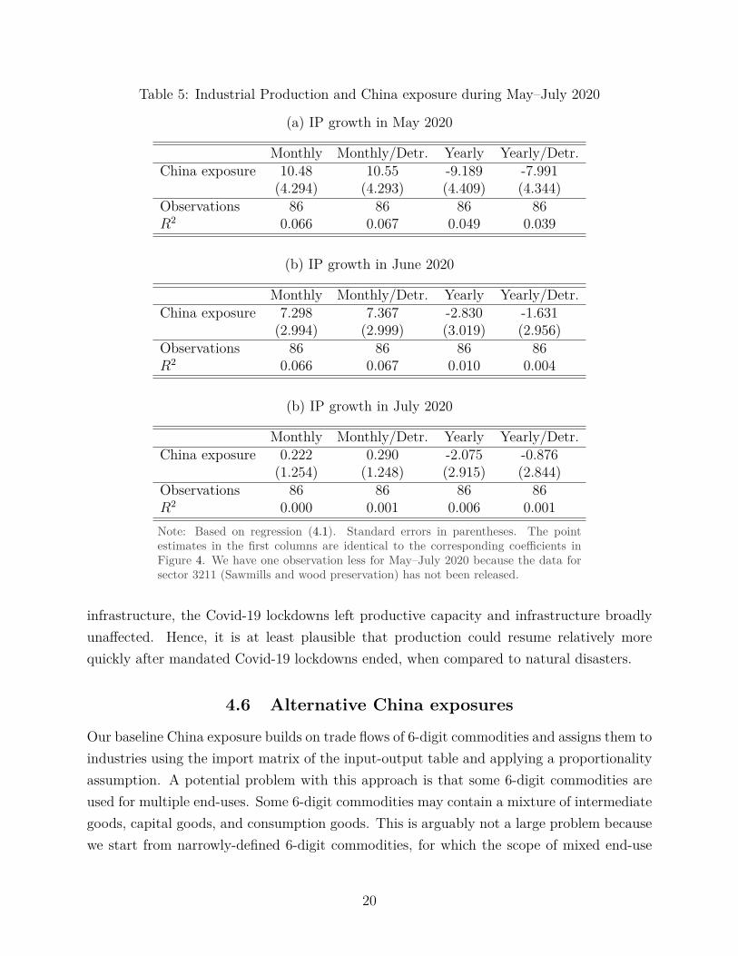
Table 5: Industrial Production and China exposure during May–July 2020

(a) IP growth in May 2020

Monthly Monthly/Detr. Yearly Yearly/Detr.China exposure 10.48 10.55 -9.189 -7.991

(4.294) (4.293) (4.409) (4.344)Observations 86 86 86 86R2 0.066 0.067 0.049 0.039

(b) IP growth in June 2020


(2.994) (2.999) (3.019) (2.956)Observations 86 86 86 86R2 0.066 0.067 0.010 0.004

(b) IP growth in July 2020


(1.254) (1.248) (2.915) (2.844)Observations 86 86 86 86R2 0.000 0.001 0.006 0.001Note: Based on regression (4.1). Standard errors in parentheses. The pointestimates in the first columns are identical to the corresponding coefficients inFigure 4. We have one observation less for May–July 2020 because the data forsector 3211 (Sawmills and wood preservation) has not been released.

infrastructure, the Covid-19 lockdowns left productive capacity and infrastructure broadlyunaffected. Hence, it is at least plausible that production could resume relatively morequickly after mandated Covid-19 lockdowns ended, when compared to natural disasters.

4.6 Alternative China exposures

Our baseline China exposure builds on trade flows of 6-digit commodities and assigns them toindustries using the import matrix of the input-output table and applying a proportionalityassumption. A potential problem with this approach is that some 6-digit commodities areused for multiple end-uses. Some 6-digit commodities may contain a mixture of intermediategoods, capital goods, and consumption goods. This is arguably not a large problem becausewe start from narrowly-defined 6-digit commodities, for which the scope of mixed end-use

20

Table 6: Exposure to intermediate good imports

(1) (2) (3) (4) (5) (6)China exposure -3.816 -14.23

(1.467) (5.016)

– BEA intermediates -9.588 -35.70(2.282) (7.719)

– BEC intermediates -5.364 -17.66(1.962) (6.780)

Observations 87 87 87 87 87 87R2 0.074 0.172 0.081 0.086 0.201 0.074Note: Based on regression (4.1). Standard errors in parentheses. Columns (1)–(3) are basedon March 2020 IP growth, columns (4)–(6) are based on April 2020 IP growth. The firstrow, China exposure, is based on all sector-specific imports from China. The second (third)row is based on constructing sector-specific imports of intermediate goods from China basedon BEA (UNSTATS BEC) classification of goods into end-use categories.

seems to be limited. To address the potential issue nonetheless, we categorize the 6-digitcommodities using either the end-use classification from the BEA or the United NationsBroad Economic Categories (BEC) classification. We then discard 6-digit commodities notclassified as intermediate inputs and proceed with the remaining commodities to constructsector-specific China exposures. It turns out that we underestimate aggregate intermediategood imports in this way. Using the BEA or BEC classification, only 37% or 45% of importsare respectively considered intermediate inputs versus 55% in the import matrix. Our empir-ical results, however, are robust to using the alternative exposure measures.

In Table 6, the first rows of panel (a) and (b) repeat the baseline April and March βt

estimates whereas the last two rows show the βt for the alternative China exposures basedon the BEA and BEC classificiations, respectively. The results are re-assuring in the sensethat the results are not dramatically different. If anything, our baseline approach seems tounderestimate the role of China exposure. In particular for the BEA-based classification,the R2 is substantially larger, which suggests that China-specific supply chain disruptionsexplain closer to 20% of the cross-sectoral variation in IP growth during March and April2020.

5 Conclusion

In this paper, we study the role of international supply chain disruptions during the Covid-19crisis. We show that US sectors with a high exposure to imports from China, significantly

21

and substantially contracted more during March and April 2020 compared to less exposedsectors. Highly exposed sectors produce less, fire more workers, export and import less,and their import and output prices increase by more. Our results suggest that differentialexposure to China-specific supply chain disruptions explain about 9% of the cross-sectoraldifferences in industrial production growth during March and April 2020. The effects appearto be relatively short-lived and become insignificant by July 2020.

ReferencesAlvarez, F., D. Argente, and F. Lippi (2020): “A Simple Planning Problem for COVID-19 Lockdown,”

CEPR Discussion Papers 14658, C.E.P.R. Discussion Papers.

Amiti, M., S. H. Kong, and D. Weinstein (2020): “The Effect of the U.S.-China Trade War on U.S.Investment,” Working Paper 27114, National Bureau of Economic Research.

Antràs, P. (2020): “De-Globalisation? Global Value Chains in the Post-COVID-19 Age,” Working Paper.

Auerbach, A. J., Y. Gorodnichenko, and D. Murphy (2020): “Fiscal Policy and COVID19 Restric-tions in a Demand-Determined Economy,” Working Paper 27366, National Bureau of Economic Research.

Bachas, N., P. Ganong, P. J. Noel, J. S. Vavra, A. Wong, D. Farrell, and F. E. Greig (2020):“Initial Impacts of the Pandemic on Consumer Behavior: Evidence from Linked Income, Spending, andSavings Data,” Working Paper 27617, National Bureau of Economic Research.

Baldwin, R. and B. W. di Mauro (2020): Economics in the Time of COVID-19, VoxEU.org eBook,CEPR Press.

Balleer, A., S. Link, M. Menkhoff, and P. Zorn (2020): “Demand or Supply? Price Adjustmentduring the Covid-19 Pandemic,” CEPR Discussion Papers 14907, C.E.P.R. Discussion Papers.

Baqaee, D. and E. Farhi (2020): “Supply and Demand in Disaggregated Keynesian Economies with anApplication to the Covid-19 Crisis,” NBER Working Papers 27152.

Barrot, J.-N., B. Grassi, and J. Sauvagnat (2020): “Sectoral Effects of Social Distancing,” CEPRCovid Economics.

Barrot, J.-N. and J. Sauvagnat (2016): “Input Specificity and the Propagation of Idiosyncratic Shocksin Production Networks,” The Quarterly Journal of Economics, 131, 1543–1592.

Bayer, C., B. Born, R. Luetticke, and G. Müller (2020): “The Coronavirus Stimulus Package: Howlarge is the transfer multiplier? ,” Cepr discussion papers, C.E.P.R. Discussion Papers.

Bigio, S., M. Zhang, and E. Zilberman (2020): “Transfers vs Credit Policy: Macroeconomic PolicyTrade-offs during Covid-19,” Working Paper 27118, National Bureau of Economic Research.

Boehm, C. E., A. Flaaen, and N. Pandalai-Nayar (2019): “Input Linkages and the Transmission of

22

Shocks: Firm-Level Evidence from the 2011 Thoku Earthquake,” The Review of Economics and Statistics,101, 60–75.

Bonadio, B., Z. Huo, A. A. Levchenko, and N. Pandalai-Nayar (2020): “Global Supply Chains inthe Pandemic,” Working Paper 27224, National Bureau of Economic Research.

Brinca, P., J. B. Duarte, and M. F. e Castro (2020): “Measuring Sectoral Supply and DemandShocks during COVID-19,” CEPR Covid Economics.

Caballero, R. J. and A. Simsek (2020): “Asset Prices and Aggregate Demand in a “Covid-19” Shock: AModel of Endogenous Risk Intolerance and LSAPs,” Working Paper 27044, National Bureau of EconomicResearch.

Carvalho, V. M., M. Nirei, Y. Saito, and A. Tahbaz-Salehi (2020): “Supply chain disruptions:evidence from the great east japan earthquake,” mimeo, University of Cambridge.

Chetty, R., J. N. Friedman, N. Hendren, M. Stepner, and T. O. I. Team (2020): “How DidCOVID-19 and Stabilization Policies Affect Spending and Employment? A New Real-Time EconomicTracker Based on Private Sector Data,” Working Paper 27431, National Bureau of Economic Research.

Choi, T. Y., D. Rogers, and B. Vakil (2020): “Coronavirus Is a Wake-Up Call for Supply ChainManagement,” Harvard Business Review.

Davis, S. J. and J. Haltiwanger (1990): “Gross Job Creation and Destruction: Microeconomic Evidenceand Macroeconomic Implications,” in NBER Macroeconomics Annual 1990, Volume 5, National Bureauof Economic Research, Inc, NBER Chapters, 123–186.

Donnan, S., C. Rauwald, J. Deaux, and I. King (2020): “A Covid-19 Supply Chain Shock Born inChina Is Going Global,” Bloomberg.

Eichenbaum, M. S., S. Rebelo, and M. Trabandt (2020): “The Macroeconomics of Epidemics,”Working Paper 26882, National Bureau of Economic Research.

Flaaen, A., A. Hortaçsu, and F. Tintelnot (2020): “The Production Relocation and Price Effects ofUS Trade Policy: The Case of Washing Machines,” American Economic Review, 110, 2103–27.

Flaaen, A. and J. Pierce (2019): “Disentangling the Effects of the 2018-2019 Tariffs on a GloballyConnected U.S. Manufacturing Sector,” Finance and Economics Discussion Series, 2019.

Fornaro, L. and M. Wolf (2020): “Covid-19 Coronavirus and Macroeconomic Policy,” CEPR DiscussionPapers 14529, C.E.P.R. Discussion Papers.

Gerschel, E., A. Martinez, and I. Mejean (2020): “Propagation of shocks in global value chains: thecoronavirus case,” IPP Policy Brief.

Glick, R. and A. M. Taylor (2010): “Collateral Damage: Trade Disruption and the Economic Impactof War,” The Review of Economics and Statistics, 92, 102–127.

Glover, A., J. Heathcote, D. Krueger, and J.-V. Ríos-Rull (2020): “Health versus Wealth: On

23

the Distributional Effects of Controlling a Pandemic,” CEPR Covid Economics.

Hassan, T. A., S. Hollander, L. van Lent, and A. Tahoun (2020): “Firm-level Exposure to EpidemicDiseases: Covid-19, SARS, and H1N1,” Working Paper 26971, National Bureau of Economic Research.

Huang, Y., C. Lin, S. Liu, and H. Tang (2018): “Trade Linkages and Firm Value: Evidence fromthe 2018 US-China “Trade War”,” IHEID Working Papers 11-2018, Economics Section, The GraduateInstitute of International Studies.

Johnson, R. C. and G. Noguera (2012): “Accounting for intermediates: Production sharing and tradein value added,” Journal of International Economics, 86, 224 – 236.

Kahn, J. A., M. M. McConnell, and G. Perez-Quiros (2002): “On the causes of the increasedstability of the U.S. economy,” Economic Policy Review, 8, 183–202.

Krueger, D., H. Uhlig, and T. Xie (2020): “Macroeconomic Dynamics and Reallocation in anEpidemic,” Working Paper 27047, National Bureau of Economic Research.

McConnell, M. M. and G. Perez-Quiros (2000): “Output Fluctuations in the United States: WhatHas Changed since the Early 1980’s?” American Economic Review, 90, 1464–1476.

Meier, M. (2020): “Supply Chain Disruptions, Time to Build, and the Business Cycle,” Discussion PaperSeries - CRC TR 224.

Mitman, K. and S. Rabinovich (2020): “Optimal Unemployment Benefits in the Pandemic,” CEPRDiscussion Papers 14915, C.E.P.R. Discussion Papers.

Nakamura, E. and J. Steinsson (2008): “Five Facts about Prices: A Reevaluation of Menu Cost Models,”The Quarterly Journal of Economics, 123, 1415–1464.

Pasten, E., R. Schoenle, and M. Weber (forthcoming): “The Propagation of Monetary Policy Shocksin a Heterogeneous Production Economy,” Journal of Monetary Economics.

Rajan, R. and L. Zingales (1998): “Financial Dependence and Growth,” American Economic Review,88, 559–86.

Roberts, I. and G. White (2015): “Seasonal Adjustment of Chinese Economic Statistics,” RBA ResearchDiscussion Papers rdp2015-13, Reserve Bank of Australia.

Schmalz, F. (2020): “The coronavirus outbreak is disrupting supply chains around the world – here’s howcompanies can adjust and prepare,” Business Insider.

Timmer, M., E. Dietzenbacher, B. Los, R. Stehrer, and G. de Vries (2015): “An IllustratedUser Guide to the World InputOutput Database: the Case of Global Automotive Production,” Review ofInternational Economics, 23, 575–605.

Woodford, M. (2020): “ Effective Demand Failures and the Limits of Monetary Stabilization Policy,”Cepr discussion papers, C.E.P.R. Discussion Papers.

24

Appendix AWe consider the problem of type 1 establishments and drop index 1 for convenience. Before theshock, the input choices are denoted by x, m, and z = x

m . After the shock, they are denoted by xt,mt, and zt = xt

mt. While the supply chain disruption constrains the choice of mt to mt = (1 − δ)m,

the input xt is chosen optimally before and after the shock. The first-order conditions for x/xt

expressed in terms of z/zt and m/mt are given by

αγmγ−1f(z)γ−ρzρ−1 = px, (A.1)

αγmγ−1t f(zt)γ−ρzρ−1

t = px. (A.2)

We combining the two first-order conditions to obtain

f(zt)γ−ρzρ−1t = (1 − δ)1−γf(z)γ−ρzρ−1. (A.3)

Taking a first-order Taylor expansion w.r.t. zt and δ at δ = 0 and hence zt = z yields

[−(1 − ρ) + (γ − ρ)ϵ] dzt

z= −(1 − γ)dδ, (A.4)

where ϵ = zf ′(z)f(z) . Using d log zt = dzt

z and d log mt ≈ −dδ, we obtain

d log zt

d log mt= − 1 − γ

(1 − ρ) − (γ − ρ)ϵ. (A.5)

Appendix B

Table 7: List of all sectors

NAICS description NAICS description1133 Logging 3273 Cement and concrete product211 Oil and gas extraction 3274 Lime and gypsum product2121 Coal mining 3279 Other nonmetallic mineral product2122 Metal ore mining 3311,2 Iron and Steel Manufacturing2123 Nonmetallic mineral mining 3313 Alumina and aluminum production213 Support activities for mining 3314 Nonferrous metal production2211 Electric power generation 3315 Foundries2212 Natural gas distribution 3321 Forging and stamping3111 Animal food 3322 Cutlery and handtool

25

3112 Grain and oilseed milling 3323 Architectural and structural metals3113 Sugar and confectionery product 3324 Boiler, Tank, Shipping Container3114 Fruit and vegetable preserving 3325 Hardware3115 Dairy product 3326 Spring and wire product3116 Animal slaughtering and processing 3327 Machine shops; turned product; screw3117 Seafood product preparation 3328 Coating, engraving, heat treating3118 Bakeries and tortilla 3329 Other fabricated metal product3119 Other food 3331 Agriculture, construction, mining3121 Beverage 3332 Industrial machinery3122 Tobacco 3333,9 Commercial and Service Industry3131 Fiber, yarn, and thread mills 3334 Ventilation, heating, AC, refrigeration3132 Fabric mills 3335 Metalworking machinery3133 Textile, fabric finishing, fabric coating 3336 Engine, turbine, power transmission3141 Textile furnishings mills 3341 Computer and peripheral equipment3149 Other textile product mills 3342 Communications equipment315 Apparel 3343 Audio and video equipment316 Leather and allied product 3344 Semiconductor, electronic component3211 Sawmills and wood preservation 3345 Navigational, measuring3212 Veneer, plywood, engineered wood 3346 Magnetic and Optical Media3219 Other wood product 3351 Electric lighting equipment3221 Pulp, paper, and paperboard mills 3352 Household appliance3222 Converted paper product 3353 Electrical equipment323 Printing, related support activities 3359 Other electrical equipment324 Petroleum and coal products 3361 Motor vehicle3251 Basic chemical 3362 Motor vehicle body and trailer3252 Resin, synthetic rubber and fibe 3363 Motor vehicle parts3253 Pesticide, fertilizer 3364 Aerospace product and parts3254 Pharmaceutical and medicine 3365 Railroad rolling stock3255 Paint, coating, and adhesive 3366 Ship and boat building3256 Soap, cleaning, toilet preparation 3369 Other transportation equipment3259 Other Chemical Product 3371 Household and institutional furniture3261 Plastics product 3372-9 Office Furniture Manufacturing3262 Rubber product 3391 Medical equipment and supplies3271 Clay product and refractory 3399 Other Miscellaneous Mfg3272 Glass and glass product 5111 Newspaper, periodical, book

Note: Some sector descriptions are shortened.

26

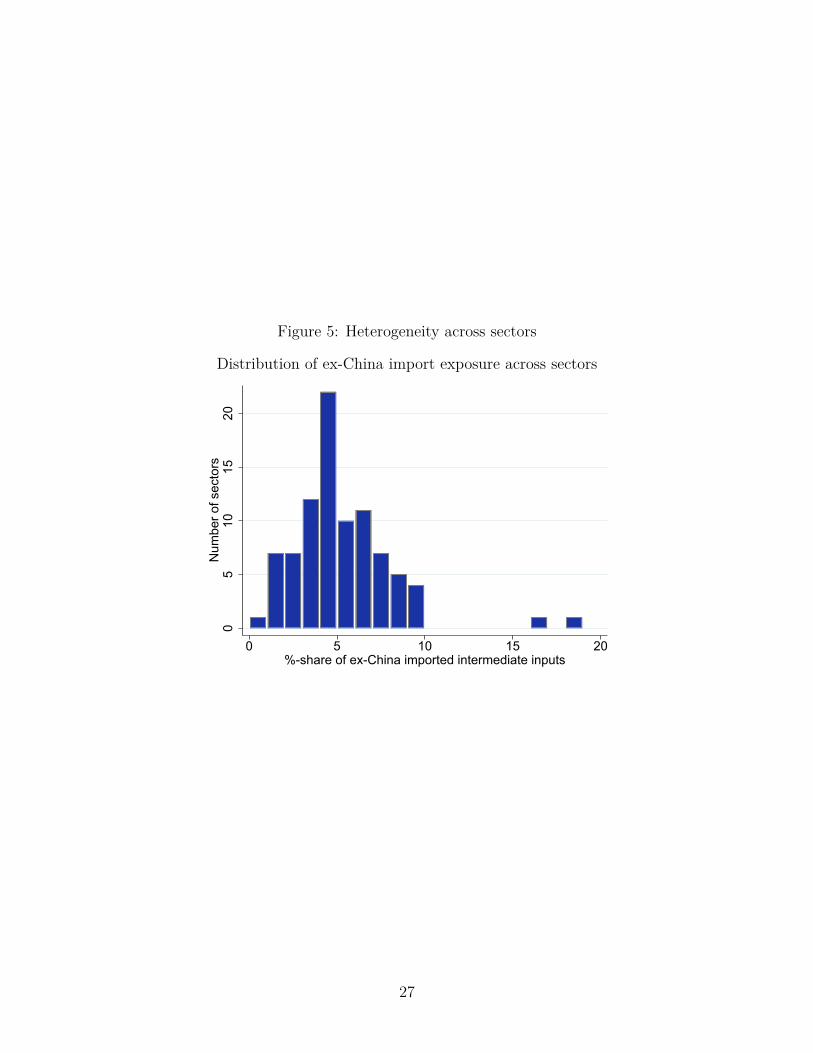
Figure 5: Heterogeneity across sectors

Distribution of ex-China import exposure across sectors

05

1015

20N

umbe

r of s

ecto

rs

0 5 10 15 20%-share of ex-China imported intermediate inputs

27

Table 8: Employment (EMP) with additional controls

(a) Employment growth in March 2020

(1) (2) (3) (4) (5)China exposure -0.227 -0.253 -0.243 -0.262 -0.328

(0.189) (0.187) (0.191) (0.196) (0.197)

Ext. Finance Dependence 0.119 0.129(0.0670) (0.0676)

Exports to China 0.00407 0.00547(0.00612) (0.00613)

Business cycle correlation 0.288 0.432(0.419) (0.422)

Observations 87 87 87 87 87R2 0.017 0.053 0.022 0.022 0.070

(b) Emploment growth in April 2020

(1) (2) (3) (4) (5)China exposure -5.732 -5.682 -6.292 -4.169 -4.653

(2.192) (2.211) (2.169) (2.185) (2.214)


Exports to China 0.143 0.114(0.0695) (0.0688)


Observations 87 87 87 87 87R2 0.074 0.075 0.119 0.152 0.183


28

Table 9: Import prices (IPI) with additional controls

(a) Import price growth in March 2020

(1) (2) (3) (4) (5)China exposure 4.991 4.943 4.645 4.208 3.522

(2.005) (2.021) (2.010) (2.061) (2.089)


Exports to China 0.0885 0.109(0.0644) (0.0649)


Observations 87 87 87 87 87R2 0.068 0.069 0.088 0.091 0.124

(b) Import price growth in April 2020

(1) (2) (3) (4) (5)China exposure 9.075 9.125 8.573 8.058 7.258

(2.976) (3.002) (2.986) (3.069) (3.120)


Exports to China 0.128 0.153(0.0957) (0.0969)


Observations 87 87 87 87 87R2 0.099 0.099 0.118 0.116 0.142


29

Table 10: Output prices (PPI) with additional controls

(a) Output price growth in March 2020

(1) (2) (3) (4) (5)China exposure 2.590 2.694 2.417 1.822 1.611

(1.609) (1.616) (1.624) (1.643) (1.678)


Exports to China 0.0443 0.0596(0.0521) (0.0521)


Observations 87 87 87 87 87R2 0.030 0.038 0.038 0.066 0.086

(b) Output price growth in April 2020

(1) (2) (3) (4) (5)China exposure 4.887 5.059 4.693 3.712 3.508

(2.667) (2.680) (2.699) (2.733) (2.800)


Exports to China 0.0498 0.0724(0.0865) (0.0870)


Observations 87 87 87 87 87R2 0.038 0.046 0.042 0.069 0.082


30

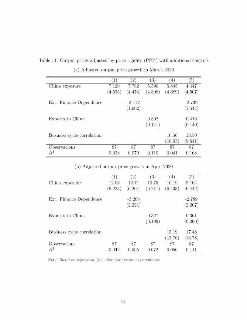
Table 11: Output prices adjusted by price rigidity (PPI∗) with additional controls

(a) Adjusted output price growth in March 2020

(1) (2) (3) (4) (5)China exposure 7.120 7.782 5.590 5.845 4.447

(4.533) (4.474) (4.398) (4.689) (4.507)


Exports to China 0.392 0.416(0.141) (0.140)


Observations 87 87 87 87 87R2 0.028 0.070 0.110 0.041 0.168

(b) Adjusted output price growth in April 2020

(1) (2) (3) (4) (5)China exposure 12.03 12.71 10.75 10.19 9.104

(6.223) (6.201) (6.211) (6.433) (6.442)


Exports to China 0.327 0.361(0.199) (0.200)


Observations 87 87 87 87 87R2 0.042 0.065 0.072 0.056 0.111


31

Table 12: Imports (IMP) with additional controls

(a) Import growth in March 2020

(1) (2) (3) (4) (5)China exposure -9.181 -9.279 -9.639 -8.137 -8.807

(3.854) (3.890) (3.865) (3.962) (4.052)


Exports to China 0.142 0.123(0.122) (0.125)


Observations 83 83 83 83 83R2 0.065 0.067 0.081 0.080 0.091

(b) Import growth in April 2020

(1) (2) (3) (4) (5)China exposure -12.73 -13.01 -13.54 -12.68 -14.26

(7.153) (7.215) (7.181) (7.410) (7.557)


Exports to China 0.249 0.261(0.227) (0.233)

Business cycle correlation -0.536 3.461(15.99) (16.39)

Observations 83 83 83 83 83R2 0.038 0.040 0.052 0.038 0.055


32

Table 13: Exports (EXP) with additional controls

(a) Export growth in March 2020

(1) (2) (3) (4) (5)China exposure -5.612 -6.014 -5.598 -4.834 -5.226

(2.543) (2.513) (2.572) (2.608) (2.631)


Exports to China -0.00426 -0.0170(0.0811) (0.0812)


Observations 83 83 83 83 83R2 0.057 0.097 0.057 0.075 0.112

(b) Export growth in April 2020

(1) (2) (3) (4) (5)China exposure -21.08 -22.25 -21.79 -17.11 -19.16

(6.343) (6.213) (6.367) (6.299) (6.287)


Exports to China 0.222 0.151(0.201) (0.194)


Observations 83 83 83 83 83R2 0.120 0.172 0.133 0.191 0.240


33

Table 14: Other outcomes

(a) Yearly growth rates in May 2020


(4.409) (2.303) (2.786) (2.186) (5.906) (8.392) (6.948)Observations 86 86 86 86 86 82 82R2 0.049 0.035 0.092 0.030 0.027 0.058 0.049

(b) Yearly growth rates in June 2020


(3.019) (1.485) (1.887) (1.333) (4.577) (6.730) (4.716)Observations 86 86 86 86 86 82 82R2 0.010 0.010 0.082 0.050 0.046 0.027 0.003

Note: Based on regression (4.1). Standard errors in parentheses. IP: industrial production growth,EMP: employment growth, IPI: import price index growth, PPI: purchaser price index growth,PPI∗: PPI growth divided by price adjustment frequency, IMP: import growth, EXP: exportgrowth.

34

Covid-19 Supply Chain Disruptions

Documents

Transcript of Covid-19 Supply Chain Disruptions