COVER PAGE - International Science Programme · 1 Herbert Fleischner Austria 41 Mohamed Eltom Sudan...

COVER PAGE

i

List of Participants

Sn. Name Country Sn. Name Country1 Herbert Fleischner Austria 41 Mohamed Eltom Sudan2 Eleonora Ciriza Italy 42 Mpinganzima Lydie Sweden3 Andrew Masibayi Kenya 43 Pravina Gajjar Sweden4 Ben Owino Obiero Kenya 44 Bjrn Textorius Sweden5 Benard Kipchumba Kenya 45 Olof Svensson Sweden6 Bernard Nzimbi Kenya 46 Bengt Ove Turesson Sweden7 Damian Maing Kenya 47 Christer Kiselman, Sweden8 David Angwenyi Kenya 48 Fredrik Berntsson Sweden9 Emma Anyika Kenya 49 Leif Abrahamsson Sweden

10 George Muhua Kenya 50 Paul Vanderlin Sweden11 Idah Orowe Kenya 51 Peter Sundin, Sweden12 Isaac Kipchirchir Kenya 52 Rikard Bogvad Sweden13 Ivivi Mwaniki Kenya 53 Vitalij Tjatyrko Sweden14 Jamen H. We’re Kenya 54 Agnes Joseph Tanzania15 James Okwoyo Kenya 55 Akili Babi Tanzania16 John Nderitu Kenya 56 Alex Xavery Matofali Tanzania17 Josephine Wairimu Kenya 57 Allen Mushi Tanzania18 Kevin Oketch Kenya 58 Anna Mwanjoka Tanzania19 Kithela Mille Kenya 59 Beatha Ngonyani Tanzania20 Lydiah Musiga Kenya 60 Charles Mahera Tanzania21 Masinde Wamalwa Kenya 61 Christian Alphonce Tanzania22 Ongaro Nyang’au Kenya 62 E. S. Massawe Tanzania23 Patrick Weke Kenya 63 Edith Luhanga Tanzania24 Philip Ngare Kenya 64 Egbert Mujuni Tanzania25 Rachel Mbogo Kenya 65 Emaline Joseph Tanzania26 Richard Simwa Kenya 66 Emmanuel Evarest Tanzania27 Waihenya Kamau Kenya 67 Eunice Mureithi Tanzania28 Wycliff Nyang’era Kenya 68 Greyson. Kakiko Tanzania29 Fanja Rakotondrajao Madagascar 69 Isambi Sailon Mbalawata Finland30 Bernard O. Ikhimwin Nigeria 70 John Mwaonanji Tanzania31 Ewaen K.y Osawaru Nigeria 71 Jonas P. Senzige Tanzania32 Cassien Habyarimana Rwanda 72 Josepha V. Itambu Tanzania33 Desire Karangwa Rwanda 73 Judith Pande Tanzania34 Froduald Minani Rwanda 74 Lilian Olengeile Tanzania35 Gahirima Michael. Rwanda 75 Mashaka Mkandawile Tanzania36 Isidore Mahara Rwanda 76 Moses Mwale Tanzania37 E Nshimyumuremyi Rwanda 77 Mpele James Tanzania38 Thomas Bizimana Rwanda 78 Mpeshe, Saul C. Tanzania39 Abdou Sene Senegal 79 Augustino Isdory Tanzania40 Oluwole Daniel Makinde S. Africa 80 Muhaya Kagemulo Tanzania

ii

Sn. Name Country Sn. Name Country81 Mussa Ally Tanzania 104 Mukalazi Herbert Uganda82 Pitos Seleka Tanzania 106 Nanyondo Josephine Uganda83 Said Sima Tanzania 107 Ndagire Majorine Uganda84 Santosh Kumar Tanzania 108 Opio Ismai Uganda85 Shaban Nyimvua Tanzania 109 Sanyu Shaban Uganda86 Silas S. Mirau Tanzania 111 Tumuramye Fred Kacumita Uganda87 Soud Khalfa Mohamed Tanzania 112 Tushemerirwe Phionah Uganda88 Sylvester E. Rugeihyamu Tanzania 113 Tushemerirwe Phionah Uganda89 Theresia Bonifasi Tanzania 114 Vincent Ssembatya Uganda90 Theresia Marijani Tanzania 115 Walakira David Ddumba Uganda91 Uledi A. Ngulo Tanzania 116 Wandera Ogana Uganda92 Yaw Nkansah-Gyekye Tanzania 117 David Henwood UK93 Anguzu Collins Uganda 118 admanabhan Seshaiyer USA94 Arop M. Uganda 119 Alasford M. Ngwengwe Zambia95 Buletwenda Charles Uganda 120 Anthony Moses Mwale Zambia96 John Mango Uganda 121 Ilwale Kwalombota Zambia97 Juma Kasoz iUganda 122 Issac. D. Tembo Zambia98 Kitayimbwa Mulindwa John Uganda 123 John Musonda Zambia99 Kito Luliro Silas Uganda 124 Mbokoma Mainza Zambia100 Likiso Remo Winniefred Uganda 125 Mervis Kikonko Shamalambo Zambia101 Livingstone Luboobi Uganda 126 Mubanga Lombe Zambia102 Masette Simon Uganda 127 Trevor Chilombo Chimpinde Zambia103 Mirumbe Geoffrey Ismail Uganda

iii

Forewords

The East African Universities Mathematics Programme (EAUMP) is a collaboration project be-tween Eastern Africa Universities and International Science Programme (ISP) of Uppsala Uni-versity, Sweden. The project started in 2002, and the currently participating universities in theregion are University of Dar es Salaam, University of Nairobi, Makerere University, NationalUniversity of Rwanda, Kigali Institute of Technology and University of Zambia. The mainobjective of the programme is to promote cooperation and exchange of ideas in mathematicalresearch and teaching of mathematics and to stimulate communication between mathematiciansin the Eastern African Region and beyond.

The first EAUMP Conference was held in Nairobi, Kenya, from 18th March to 21st March2003. Due to the success of the conference it was decided to hold such a conference regularly.The Department of Mathematics of the University of Dar es Salaam agreed to hold the 2ndEAUMP conference to celebrate 10th anniversary of the programme.

The proceedings, which follow, consist of speeches, papers and abstracts presented at the 2ndEAUMP Conference, held at The Nelson Mandela African Institute of Science and Technology,Arusha, Tanzania from 22nd to 25th August 2012. More than 125 participants from about 10countries attended the conference. The conference program was comprised of 6 invited plenarylectures, and more than 45 contributed talks were presented and discussed.

The aims of the conference were:

• To stimulate regional and international collaboration in research and training.

• To provide a forum for interaction of African Mathematicians and others from the devel-oped countries for research experience.

• To introduce African Mathematicians from the region to some fundamental techniquesand recent developments in these fields, thus forming research collaborations.

• To update the knowledge of African Mathematicians, particularly lecturers and M.Sc../Ph.D.students who are stationed at home, to start pursuing these areas as research interest.

The success of the conference could not have been registered without concerted effort from theLocal organizing committee in the Department of Mathematics and the EAUMP coordinatorscommittee. I would therefore like to extend my heartfelt thanks to the following.

Local Organizing Committee

• Dr. Egbert Mujuni Chairperson

• Dr. Sylvester. E. Rugeihyamu EAUMP coordinator

• Dr. Eunice Mureithi Member

• Dr. Theresia Marijani Secretary

• Mr. Emmanuel Evarest Member

iv

EAUMP Coordinating Committee

• Dr. Sylvester E. Rugeihyamu (Coordinator of University of Dar es Salaam)

• Prof. Patrick G. O. Weke (Coordinator of University of Nairobi)

• Dr. Juma Kasozi (Coordinator of Makerere University)

• Dr. Isaac Tembo (Coordinator of University of Zambia)

• Dr. Isidore Mahara (Coordinator of National University of Rwanda)

• Mr. Michael Gahirima (Coordinator of Kigali Institute of Science and Technology)

• Dr. John M. Mango (Inter Network Coordinator, Makerere University)

AcknowledgementWithout finances, not much could have been attained. I would like extend my thanks followingassociations, agencies and institutions for their generous support.

• International Science Programme (ISP) of Uppsala University, Sweden.

• TWAS-The Academy Science of the Developing World.

• The International Mathematical Union-Committee for Developing Countries (IMU CDC).

• NORAD (Through NOMA Project in Mathematics Department, UDSM).

• The German Academic Exchange Service (DAAD).

• University of Dar es Salaam Gender Centre.

• University of Dar es Salaam, Directorate of Research.

• Tanzania Communications Regulatory Authority (TCRA).

• Tanzania Commission for Science and Technology (COSTECH).

Prof. E. S. Massawe

Head, Mathematics Department, UDSM and Overall EAUMP Coordinator

v

Contents

List of Participants ii

Forewords iv

SPEECHES 1

Prof. E. S. Massawe: Welcome Speech . . . . . . . . . . . . . . . . . . . . . . . . 1

Dr. John M. Mango: Eastern Africa Universities Mathematics program (EAUMP -Network Origin, Operation, Achievements the Future and Challenges. . . . . . 3

Prof. Rwekaza Mukandala: Welcome Speech . . . . . . . . . . . . . . . . . . . . 8

Prof. Makame Mnyaa Mbarawa: OPENING SPEECH . . . . . . . . . . . . . . . 9

PAPERS 11

M. E. A. El Tom: A Proposed Research Agenda in Mathematics Education in Africa 11

Paul Vaderlind: Mathematical Competitions for Gifted Students: Organization andTraining . . . . . . . . . . . . . . . . . . . . . . . . . . . . . . . . . . . . . . 23

Patrick G. O. Weke: Estimation of IBNR Claims Reserves Using Linear Models . . 26

O. D. Makinde: Heat Transfer Analysis of a Convecting and Radiating Two StepReactive Slab . . . . . . . . . . . . . . . . . . . . . . . . . . . . . . . . . . . 43

Mervis Kikonko: Non-Definite Sturm-Liouville Problems Two Turning Points . . . 52

S. A. Sima, M. Ali and I. Campbell: The Three Layers Maize Crop Optimal Distri-bution Network in Tanzania . . . . . . . . . . . . . . . . . . . . . . . . . . . . 61

Santosh Kumar: A Survey of the Development of Fixed Point Theory . . . . . . . . 72

Livingstone S. Luboobi: Epediomological Modelling at Macro and Micro Levels:The Case of HIV/AIDS . . . . . . . . . . . . . . . . . . . . . . . . . . . . . . 81

Christian Baruka Alphonce: Analysis of Cell Phone User’s Loyalty in TanzaniaUsing Markov Chains . . . . . . . . . . . . . . . . . . . . . . . . . . . . . . . 87

Soud K. Mohamed: Derivatives over Certain Finite Rings . . . . . . . . . . . . . . 98

Eleonora Ciriza: Bifurcation results on symplectic manifolds . . . . . . . . . . . . 108

John Musonda: Three Systems of Orthogonal Polynomials and Associated Operators 120

ABSTRACTS 155

Christer Kiselman: Asymptotic Properties of The Delannoy Numbers andSimilar Arrays . . . . . . . . . . . . . . . . . . . . . . . . . . . . . . 155

Vitalij A. Chatyrko: The (Dis)connectedness of Products in the Box Topology 155

vi

Frerik Berntsson: Identification of Coefficients in Parabolic Equations UsingMeasurements on the Boundary . . . . . . . . . . . . . . . . . . . . . 155

Padmanabhan Seshaiyer: Multidisciplinary Research in Mathematical Sci-ences With Applications to Real World Problems in Biological, Bio-Inspired and Engineering Systems . . . . . . . . . . . . . . . . . . . . 156

Wandera Ogana: Epidemic Potential for Malaria in Epidemiological Zones inKenya . . . . . . . . . . . . . . . . . . . . . . . . . . . . . . . . . . . 156

Fanja Rakotondrajao,: How to Manipulate Derangements . . . . . . . . . . . 156

Abdou Sene: The Dynamics of Populations in Wetlands . . . . . . . . . . . . 157

Isambi Sailon Mbalawata and Simo Sarkka: Adaptive Markov Chain MonteCarlo Using Variational Bayesian Adaptive Kalman Filter . . . . . . . 157

Patrick G. O. Weke: Linear Estimation of Location and Scale Parameters forLogistic Distribution Based on Consecutive Order Statistics . . . . . . 158

Lydia Musiga: A Stochastic Model for Planning a Compartmental EducationSystem and Supply of Manpower . . . . . . . . . . . . . . . . . . . . 158

Emma Anyika and Patrick Weke: Financial Sector Performance Enhancers . 158

Mashaka Mkandawile: Estimating the List Size Using Bipartite Graph forColouring Problems . . . . . . . . . . . . . . . . . . . . . . . . . . . 159

Emaline Joseph, Kgosimore and Teresia Marijani: Mathematical Modelingof Pneumonia Transmission Dynamics . . . . . . . . . . . . . . . . . . 159

David Ddumba Walakira: Hydrodynamics of Shallow Water Equations: ACase Study of Lake Victoria . . . . . . . . . . . . . . . . . . . . . . . 159

J.W. Mwaonanji: Boundary Layer Flow Over a Moving at Surface With Tem-perature Dependent Viscosity . . . . . . . . . . . . . . . . . . . . . . 160

Eunice Mureithi: Absolute-Convective Instability of Mixed Forced-Free Con-vection Boundary Layers . . . . . . . . . . . . . . . . . . . . . . . . . 160

Moses Mwale: Optimal Premium Policy of an Insurance Firm With Delay . . . 160

G.I. Mirumbe, Vincent SSembatya, Rikard Bgvad and Jan Erik Bjork: Onthe Coexistence of Distributional and Rational Solutions for OrdinaryDifferential Equations With Polynomial Coefficients . . . . . . . . . . 161

Philip Ngare: On Modelling and Pricing Index Linked Catastrophe Derivatives 161

Lusungu Mbiliri, Charles Mahera, and Sure Mataramvura: Optimal Port-folio Management When Stocks are Driven by Mean Reverting Processes162

Egbert Mujuni: On Hub Number of Hypercube and Grid Graphs . . . . . . . 162

Vincent A Ssembatya: Fixed Points of Homeomorphisms of Knaster Continua 162

Isaac Daniel Tembo: Continuity of Inversion in the Algebra of Locality - Mea-surable Operators . . . . . . . . . . . . . . . . . . . . . . . . . . . . . 163

vii

Herbert Fleischner: Uniquely Hamiltonian Graphs . . . . . . . . . . . . . . . 163

Kitayimbwa M. John, Joseph Y. T. Mugisha and Robert A. Saenz: TheRole of Backward Mutations on the Within Host Dynamics Of HIV-1 . 163

Kipchirchir, I. C.: Comparative Study of the Distributions Used To ModelDispersion . . . . . . . . . . . . . . . . . . . . . . . . . . . . . . . . 164

Theresia Marijani: A Within Host Model of Blood Stage Malaria . . . . . . . 164

Wilson Mahera Charles: Application of Stochastic Differential Equations toModel Dispersion of Pollutants in Shallow Water . . . . . . . . . . . . 165

R. W. Mbogo, L. LuboobiJ. W. Odhiambo: Stochastic Model for In-HostHIV Virus Dynamics With Therapeutic Intervention . . . . . . . . . . 165

F. Berntsson, V. Kozlov, L. Mpinganzima, and B.O. Turesson: An Alter-nating Iterative Procedure for the Cauchy Problem for the HelmholtzEquation . . . . . . . . . . . . . . . . . . . . . . . . . . . . . . . . . 165

viii

THE 2ND EASTERN AFRICA UNIVERSITIES MATHEMATICSPROGRAMME (EAUMP) CONFERENCE

The Nelson Mandela African Institute of Science and Technology, Arusha, TanzaniaAugust 22nd - 25th, 2012

Welcome Speechby

Prof. E. S. Massawe

Head, Mathematics Department, University of Dar Es Salaam

Guest of Honour, Minister of Communication, Science & Technology, Tanzania, Hon. Prof.Makame Mnyaa Mbarawa (MP),

The Vice Chancellor of the University of Dar es Salaam, Professor Rwekaza Mkandala

The Vice Chancellor Nelson Mandela African Institute of Science and Technology, ProfessorBurton Mwamila

Head of ISP and Director of Chemistry Program, Professor Peter Sundin

Director of Mathematics Program, Professor Leif Abrahamsson

Delegates from ISP

Distinguished guests and visitors,

Dear Participants,

Ladies and Gentlemen,

On behalf of the Department of mathematics, University of Dar es Salaam and on my ownbehalf, I wish to take this opportunity to welcome you all the invited guests and participantsand especially you the guest of honour, the Minister of Communication, Science & Technology,Tanzania, Hon. Prof. Makame Mnyaa Mbarawa, to this important Congress. Please do feel athome.

Guest of HonourThe Eastern Africa Universities Mathematics Programme (EAUMP) Network was establishedin 2002 to further the mathematical sciences in the Eastern Africa Region. The main objectiveof the Network is to promote cooperation and exchange of ideas in mathematical research andteaching of mathematics and to stimulate communication between mathematicians in the East-ern Africa Region and beyond. The Network, since its foundation, has been organizing schoolsand workshops and conferences. One of the objectives of these workshops and conferences isto bring together researchers from various branches of mathematics and related fields, and tosimulate intersection and cooperation.

Guest of HonourEAUMP is a non-political and non-profit making Network devoted to the promotion of re-search, teaching and learning of mathematics at all levels. We are very proud of this becauserecent years have seen unprecedented growth of interest in the application of mathematicalideas and techniques to problems in Science and Technology in industry.

1

Guest of HonourEAUMP is aware of the important role of the mathematics researchers in promoting the subject.In this conference, we shall have a series of presentations and group discussions in the areas ofpure mathematics, Financial Mathematics, Epidemiology, Mathematics for the Industry, Theo-retical Fluid Dynamics, Statistics, Mathematics Education, Computer Science and TheoreticalPhysics. The program will include keynote speakers, esteemed researchers and regular presen-tations.

Guest of HonourEAUMP was found in 2002. This year we are celebrating the 10th Anniversary of the EAUMPNetwork. Performance of EAUMP in the last 10 years gives one confidence that the EAUMPwill survive the next 10 years and beyond as an important and active Network. Schools andConferences of this type will have to continue. Schools and Conferences of EAUMP are thelifeline of the Network as is the case of most professional organizations

Guest of HonourFinally I will like to say that, our motto is ”We build for the Future”. The future success ofEAUMP will depend on the continued cooperation and commitment of all the members ofEAUMP and other stakeholders.

Guest of HonourAllow me on behalf of all the EAUMP members to thank all those who in various ways havesupported our Conference and specifically the International Science Programme (ISP) of Upp-sala University, Sweden , The Ministry of Communication, Science and Technology, Tanzania,Commission for Science and Technology (COSTECH), Tanzania, The Academi Science of theDeveloping World (TWAS), The European Mathematical Society - Committee for Develop-ing Countries (EMS-DC), The German Academic Exchange Service (DAAD), The Universityof Dar es Salaam, The University of Dar es Salaam Gender Centre, the University of Dar esSalaam Directorate of Research, NORAD through NOMA Project, Tanzania CommunicationsRegulatory Authority (TCRA) and All nodes of the EAUMP network

I would also like to thank the local organizing committee and all those behind the scene for theexcellent job done in terms of making us stay in Arusha happily.

Once again, you are all warmly welcome.

Thank you.

2

Eastern Africa Universities Mathematics program (EAUMP - NetworkOrigin, Operation, Achievements the Future and Challenges.

by

Dr. John M. Mango

EAUMP Coordinator and Inter-Network Cooperation

Today is a great and memorable day for EAUMP

• In June 1995, SIDA/SAREC and Uppsala University organized a conference on ’Donorsupport to development oriented research in Basic Sciences’.

• In March 1999 a conference was organized in Arusha, Tanzania with the aim of address-ing the regional challenges.

• In 2001 SIDA/SAREC organized the 1st International conference in Mathematics inAfrica South of the Sahara. It was during this conference that the poor state of Math-ematics in the Eastern African region was reported. This gave birth to EAUMP in 2002to try and address the Challenges of the time. It is interesting to note that some of thechallenges are still existing though at a reduced level.

The Key People who participated in the initial stages 2001/2002

• Prof. Leif Abrahamson -Uppsala University in Sweden.

• Dr. C. Baruka Alphonce -University of Dar es Salaam.

• Prof. V. Masanja -University of Dar es Salaam.

• Prof. John W. Odhiambo -University of Nairobi.

• Prof. Wandera Ogana -University of Nairobi.

• Dr. Vincent Ssembatya -Makerere University.

• Prof. Livingstone Luboobi -Makerere University.

• Dr Fabbian Nabugoomu, Makerere University.

Objectives of the EAUMP Network

• Enhancement of postgraduate training with special emphasis to PhD training.

• Establishing and strengthening collaborative research in Mathematics.

• Strengthening the collaborating Mathematics departments.

• Development of resources for the collaborating Mathematics Departments.

3

Membership of the Network

• University of Dar-es-Saalam, Tanzania, (Since 2002)

• Makerere University, Uganda, (Since 2002)

• University of Nairobi, Kenya. (Since 2002)

• National University of Rwanda (NUR) and Kigali Institute of Science and Technology(KIST), joined in August 2008.

• University of Zambia, joined in April 2009.

• NB: University of Addis Ababa, University of Khartoum and Nelson Mandela AfricanInstitute for Science and Technology have expressed interest to join the Network.

Coordination Structure

• ISP Mathematics Director–Prof. Leif Abrahamsson

• EAUMP Advisory Board

• Overall Coordinator–Prof Estomih Massawe (Dar-Main Coordinating office for now)

• Inter Network Coordinator– Dr John Mango Magero

• School of Mathematics, University of Nairobi Coordinator– Prof Patrick Weke

• Makerere University, Department of Mathematics Coordinator-Dr Juma Kasozi

• University of Dar es Salaam, Department of Mathematics Coordinator-Dr SylvesterRugeihyamu

• Kigali Institute of Science and Technology (KIST), Department of Applied MathematicsCoordinator-Mr Gahirima Michael

• National University of Rwanda (NUR), Department of Applied Mathematics Coordinator-Dr Mahara Isidore

• University of Zambia, Department of Mathematics Coordinator-Dr Isaac Tembo.

Sources of funding for the Network

• ISP-International Science Program (Over 95% of EAUMP activities are sponsored byISP), based at the University of Uppsala, Sweden.

• ICTP-International Centre for Theoretical Physics in Italy.

• AMMSI-Millenium Science Initiative

• LMS- London Mathematical Society

4

• DAAD

• IMU/ CDC- International Mathematical Union through its Commission for developingCountries

• TWAS-The Third World Academy of Sciences

• The other sources of sponsorship are the local universities.

Major Achievements of the Network since 2002

• Capacity building through Ph.D training (6 completed and 12 ongoing)- All are membersof staff eg Egbert Mujuni.

• Capacity building through Postdoc (4 awarded in 2011)- All are members of staff.

• Capacity building through M.Sc. training (more than 50 have benefited)- Some are mem-bers of staff, Some doing Ph.Ds. Staff exchange in the region.

• Research visits by Cooperating Scientists (From Sweden, Italy, USA,) eg Paul, Rikard,Fanja Eleonara, Ramadas etc Equipment (Computers, projectors etc).

• Books and Journals (Subscribed to some Journals, obtained books and ebooks).

• Publications (Increased volume of publication in refereed journals).

• Conferences/Workshops/Schools for graduate students and researchers/lecturers. TheSchools are organized to cover areas of mathematics where the region is most disadvantaged)-Over 300 different M.sc and some Ph.Ds have attended and benefitted from the EAUMPSchools and Conferences.

• Research projects.

• Established/identified potential of member departments.

Challenges

• Low funding and yet in this region of the world we are not short of interested students todo Masters and Ph.Ds in Mathematics.

• Insufficient local manpower to teach and supervise

• Understaffing in Departments of member universities.

• Low interest of Ph.D students in Pure Mathematics.

The future of EAUMP Network

5

• The poor state of mathematics in the region is now improved by ISP intervention. Thepresent state needs to be improved further through continued cooperation with ISP andother organizations.

• There is great need for more capacity building in the member Departments through Ph.D,PostDoc and M.Sc training.

• When resources allow, the EAUMP network will be extended to other Universities in theregion. There are smaller universities in the region where capacity building in Mathe-matics is of urgent need.

• We need to use the Network to help reduce the problem of brain drain. From the presentexperience, students who register in their local universities for their graduate trainingunder the sandwich mode, have settled, and are teaching/working in their local/regionalUniversities.

• We plan to hold a Conference in each financial cycle (3 years as was the original plan)so that our graduate students, staff and academics outside the region will gather to shareresearch experiences through paper and poster presentations.

• Strengthen the fundraising drive for the network and research cooperation with othernetworks through the newly created office of Inter Network Cooperation. Apart fromthe usual funding from ISP, ICTP and AMMSI/LMS for schools and conferences, thisyear using the new office we have been able to secure funds from CDC,TWAS and DAADand this has supported a total of 13 persons (regional speakers and DAAD Alumni).

• Improve on the way we transport our student participants to EAUMP Schools and Con-ferences. In the recent past we have lost students in road accidents while travelling toattend EAUMP Schools.

• We request for more support from our local Universities and Governments.

Just a comment

In some discussion at the 2012 European Congress of Mathematicians, one Professor criti-cized the Scandevian Sandwich training mode of Sida and ISP type practiced in Africa. Theprofessors proposal was that Sida and ISP sends money to South African Universities for ca-pacity building of the SIDA/ISP collaborating Universities in Africa so that the training of thesandwich students takes place in South African Universities and not Swedish Universities. AsEAUMP, we are strongly opposed to the idea in that;

(i) South Africa is still interested in our PhD products/graduates and Sweden is not for theyhave more than enough. The SIDA/ISP collaboration with African Universities is forcapacity building in the collaborating Universities and not in South Africa, Europe, USAetc. It is clear that South Africa has offered some of our graduates well paying positionsand these have not come back to meet the objective of the training

(ii) All the sandwich PhD students trained so far under SIDA/ISP have remained and areserving their home Universities. A case example is the SIDA Makerere Bi-Lateral pro-grammes since 2002 which has trained over 200 PhDs mostly in the hard Sciences like

6

Engineering, Medicine, Agriculture etc and all these are stationed and serving MakerereUniversity.

(iii) The cost of ISP sandwich PhD training is cheap and affordable.

We also recognize and appreciate the contribution of South African Universities in capacitybuilding of regional Universities and we hope to continue collaborating with them but not tosubstitute the SIDA/ISP collaboration. As EAUMP, we remain grateful to our sponsors, wepromise to work and achieve the set objectives as we also look forward to continued support ofthe Network by ISP and other organizations.

THANK YOU

7



Welcome Speechby

Prof. Rwekaza Mukandala

Vice Chancellor, University of Dar Es Salaam

Guest of Honour, The Minister of Communication, Science & Technology, Tanzania, Hon. Prof.Makame Mnyaa Mbarawa (MP),

Congress Participants,

Ladies and Gentlemen,

On Behalf of the entire University of Dar es Salaam and on my behalf, I wish to take thisopportunity to welcome all the invited guests and participants to this second Eastern AfricaUniversities Mathematics Programme Congress (EAUMP). Please do feel at home.

The University of Dar es Salaam is proud to host this second EAUMP Congress. I am informedthat the Network of EAUMP started on 2002, earlier than in most other regions in Sub-SaharanAfrican region. This programme is unique and flexible since it has led to close collaborationbetween the participating departments in the network. All indications have shown that thereis now more interaction among members of departments of Mathematics in the region andMathematicians from Sweden and other areas.

When the Department of Mathematics of the University of Dar es Salaam indicated to methat University of Dar es Salaam has been honoured to host the 2nd EAUMP Congress wewelcomed the initiative.

Congress of this nature complements the status of our respected and oldest Institutions inAfrica. We also know that congresses of this nature are a forum for dissemination of infor-mation and for forging meaningful cooperation and collaboration in research and teaching.Our Universities in the region encourages collaboration among scholars of same discipline andalso encourages inert-disciplinary arrangements.

At this juncture I wish to pay glowing tribute to the Swedish Universities, in particular UppsalaUniversity through Sida for their commitment in the Development and Education in our region.We in the developing countries are very grateful for the support that Sida has extended to ourUniversities for collaborative research with scientists at similar Swedish institutions. We havedeveloped capacity and competence in teaching and research.

To you participants of the congress; I wish you productive deliberations. Your contributionswill go a long way in promoting the subject of Mathematics.

I now like to take this opportunity to invite our Guest of Honour, Hon. Prof. Makame to addressyou and officially open the Congress.

8



OPENING SPEECHby

Prof. Makame Mnyaa Mbarawa

Minister Of Communication, Science & Technology, Tanzania

The Chairperson of the EAUMP Conference Organising Committee,Distinguished guests,Distinguished Conference Participants,Ladies and Gentlemen,

It is a great honour and pleasure for me to participate in this special activity of the Eastern AfricaUniversity Mathematics Programme Network. This meeting of the EAUMP is significant notonly to Mathematicians in higher learning institutions but also to all people who understand thevalue and role of mathematical Sciences in our everyday life and work. That is why I considerthis opportunity to interact with members of this Network a significant one and quite enriching.I must therefore thank the organizing committee for inviting me to participate in this openingsession and therefore allowing me time to have a glimpse at some on the professional concernsof mathematicians as reflected in the agenda for this meeting.

I take this opportunity to welcome you all to the Nelson Mandela African Institute of Scienceand Technology and to the EAUMP conference on particular. It is my sincere hope that youwill find this venue a convenience place for the kinds of activities scheduled for this conference.This is the most favourable season for this part of Tanzania. Those of you coming from warmerregions may therefore find this to be the best time of the year to visit Arusha. I am howeverconfident that, in the course of your stay, each one of you will find a memorable aspect of lifeand places in this town.

ChairpersonI am informed that during this conference, research papers on various topics in mathematics andmathematical sciences will be presented by experts in the field. I have no doubt that the papersto be presented originate from concerted research effort, and that this conference thereforeserves as an avenue for the dissemination of the findings of recent research. Yet, while sharingof ideas and research findings among yourselves is in itself a sufficiently noble activity, a lotmore will be gained if your deliberations ultimately find a place in professional publications. Ihope this is indeed what you plan to do with the papers to be presented here.

ChairpersonI wish to relate to the significant of Mathematical sciences in human experience and develop-ment. It is common knowledge that Mathematical reasoning occupies a core position in thefoundation of scientific and technological developments that have characterized the entire his-tory of humanity. It is no wonder, therefore, that mathematics is known as the queen of scienceand technology. But we also know that at the very elementary level, Mathematics is used in

9

measurements, commerce, engineering, and as a daily language of comparison. I am told, and Ihave no reason to doubt the fact that, at the most and the more sophisticated level, mathematicsis used as a tool to understand the universe. The whole of Information Technology, so we areinformed, is basically the mathematics of wave transmission. It is in view of this profound sig-nificance of the discipline of mathematics that I revere the work being done by your Networkin advancing the frontiers of knowledge in this field. I urge you to maintain vigour and rigourin researching the various topical issues of our day and in improving the public rendering ofthe nature and role of Mathematics in our lives.

ChairpersonIt is gratifying that EAUMP is a regional Network of scientists, and that it has functioned for10 years. I congratulate you for being one of the oldest and vibrant professional organizationsin our region. I also congratulate you for the excellent tradition you have instituted of holdingyour workshops in the various countries of the region rather than having them convenientlyhosted by one country. This is surely a virtue for other regional Networks to emulate.

ChairpersonI am informed that EAUMP was found in 2002, implying that the Network today is 10 yearsold, and that since then it has held several workshops. I must commend EAUMP for maintain-ing a strong and stable momentum for 10 years. I strongly join hands with you chairpersonthat;performance of the EAUMP in the last 10 years gives one confidence that EAUMP willsurvive the next 10 years and beyond as an important and active Programme.

ChairpersonI understand that in the last workshops, participants drew a list of recommendations or actionpoints. It would be interesting to explore the extent to which those have been implemented.While I am not sure it is in your interest to engage in this kind of exercise at this point intime, I am quite convinced that this would be a useful thing to do. In same vein, I may go a stepfurther and propose that you revisit all the major recommendations made in previous workshopswith a view to assessing the impact they have had on the development of Mathematics andmathematical Sciences in the region.

ChairpersonI am sure this opening session is not meant for long speeches. I therefore wish to end myremarks by wishing you very productive deliberations and a happy stay in Tanzania.

Lastly, the Chairperson, distinguished guests, ladies and gentlemen, it is now my honour andpleasure to declare the 2012 EAUMP CONFERENCE OFFICIALLY OPENED.

I thank you all for your attention

10

A Proposed Research Agenda in Mathematics Education in Africaby

M. E. A. El Tom

Garden City College for Science and Technology, Sudan

Abstract

Efforts at capacity building in mathematics in Africa have not been sufficiently sensi-tive to the importance of mathematics education. They do not appear to have been informedby the fact that mathematical research and mathematics education are organically linked: aweakness in either will undermine the other as well as the science and & technology base,which is vital for meaningful sustainable development.

The paper attempts to identify the most pressing issues and questions for mathematicseducation in Africa. The proposed research agenda in mathematics education are based onthese issues and questions.

1. IntroductionA major aim of the East African Universities Mathematics Programme (EAUMP) network is tostrengthen mathematical research in departments of mathematics participating in it. It is usefulto think of this aim as part of the broader goal of promoting mathematics in the continent,which is shared in common by the African mathematical community. The achievement of thisgoal is far from straightforward and requires considerable effort. For, mathematics in Africais ’young’ (most African countries could not boast a single Ph. D. in mathematics at the timeof independence in early 1960s. Moreover, the role of mathematics in society is ”subtle andnot generally recognised in the needs of people in everyday life and most often it remainstotally hidden in scientific and technological advancements” (Brown 2007). I consider in thenext section some specific obstacles that seem to stand between African mathematicians andthe achievement of the goal of promoting mathematics. Also, the section cites some of theproblems facing mathematics in specific African countries. The level of research output inmathematics education in Africa is discussed in section 3. A review of the literature dealingwith factors that play a role in mathematics achievement is presented in section 4. A proposedresearch agenda in mathematics education in Africa are presented in the final section.

2. Some problems of mathematics in AfricaThe International Mathematical Union (IMU) observes in a recent study that in most Africancountries ”mathematical development is limited by low numbers of secondary school teachersand mathematicians at the masters and PhD levels.” Furthermore, the study observes that ”Tal-ented students are dissuaded from careers in mathematics by low salaries, a poor public image,and a shortage of mentors engaged in exciting mathematical challenges” (IMU 2009).

Overall, the IMU study concludes, ”the story of mathematical development in Africa is one ofpotential unfulfilled. Based on the achievements of some outstanding individuals and institu-tions, it is clear that no African country lacks talented potential mathematicians. But withouta stronger educational structure at all levels, few of them are able to reach their potential.”The last statement in this quotation is further articulated in the observation that there is an

11

almost universally held conviction held by mathematicians and mathematics educators, ”thateach mathematical level of learning is grounded pyramid-like in the previous ones, and thatlack of quality or capacity at any level of a country’s mathematical infrastructure weakens allthe levels above. Conversely, the absence of some kind of pinnacle deprives the lower levels ofleadership, training and context” (IMU 2009).

2.1 Cracks in the foundation

There are important indications that educational systems in most African countries exhibitcracks in their respective systems. Awareness of these cracks and devising appropriate mea-sures for dealing with them are prerequisites for effective promotion of mathematics in thecontinent.

• Image of mathematics

Achievement in mathematics is influenced by, among other factors, beliefs about andattitudes towards mathematics. How do parents, teachers and students themselves viewmathematics? Do these groups attribute success in mathematics largely to ability or ef-fort? A questionnaire was designed and distributed to 24 leading mathematicians work-ing in departments of mathematics in universities of different African countries to try andfind answers to such questions. The response was highly limited, only 6 questionnaireswere completed and returned: Ghana, Mali, Kenya, Nigeria, Sudan and Tunisia. Theresponses from 4 of these countries, namely Ghana, Mali, Nigeria and Sudan turned outto be similar and they are presented in Figure 1.

Although it is not permissible to generalize on the basis of very limited response to thequestionnaire, the Figure suggests that general education students in Ghana, Mali, Nige-ria and Sudan have a negative image of mathematics, characterizing it as very difficult,unrelated to reality and only for the clever. Also, society in the four countries seem toshare in common with general students the perception that mathematics is both difficultand only for the clever. In contrast, policy-makers seem to have a positive image ofmathematics, indicating awareness of its importance for economic development. Indeed,the Nigerian Federal Minister of Education said ” there could be no meaningful progressin the country without promoting the study of mathematics and sciences” (AfricaSTI. 4March 2012)

Response to the questionnaire from Tunisia indicate that both general education studentsand society at large perceive mathematics as very difficult and unrelated to reality. Also,policy-makers view mathematics as very important for economic development.

In Tanzania, mathematics is characterized as Math characterized as the ”(most) diffi-cult subject taught in schools” (Philemon 2010). In their review of the strengtheningmathematics and science in secondary education (SMASSE) science project in Kenya,Onderi and Malala (2011) believe that the documented poor performance of students inmathematics could be attributed to students’ negative attitude towards the subject. Theygo on to ascribe this attitude to ”low entry behavior, belief that these subjects are hard,peer pressure, lack of proper learning facilities, teacher absenteeism and theoretical ap-proach to teaching mathematics.” However, the response to the questionnaire indicatethat policy-makers in Kenya attach great value for mathematics.

12

The data reported above pertain to 7 countries belonging to different regions of the con-tinent (North, East and West Africa), exhibit important differences in their educationalsystems, and differ in the levels of their respective economic development. Thus, it isnot unreasonable to conclude that the image of mathematics in most African countries issimilar to that reported for the 7 countries mentioned above.

Figure 1: : General education students’, society’s and policy-makers’ image of mathematics,selected African countries, 2012

General educa-tion students

Society at large Policy-makers

Very difficultUnrelated to realityOnly for the cleverVery important forpassing examinationsVery important foreconomic development

Source: responses to questionnaire from mathematicians in Ghana, Mali, Nigeria, and Sudan.

• Teachers of mathematics

Hanushek and Rivkin (2006) make the important observation that ”The most consistentfinding across a wide range of investigations is that the quality of the teacher in theclassroom is one of the most important attributes of schools”. Yet the identification ofgood teachers has been complicated by the fact that the simple measures commonly used-such as teacher experience, teacher education, or even meeting the required standards forcertification - are not closely correlated with actual ability in the classroom (Harbisonand Hanushek (1992); Hanushek (1995); Hanushek and Luque (2003); Hanushek andRivkin (2006)). But, however one perceives of good teaching (e.g. Goe (2007), there isdata to suggest strongly that ’good’ teachers of mathematics are in short supply in mostAfrican countries.

Indeed, in most African countries, mathematical development is limited by low numbersof secondary school teachers and mathematicians at the masters and PhD levels. Animportant contributing factor to this situation is that talented students are dissuaded fromcareers in mathematics by low salaries, a poor public image, and a shortage of mentorsengaged in exciting mathematical challenges (Developing Countries Strategies Group(DCSG), 2009). South Africa, Tanzania and Uganda provide examples of this problem.

In South Africa, Adler (1994) reported that “72% of mathematics teachers in Africanschools, are under-qualified ” Obviously, these shortages of 18 years ago pose an enor-mous challenge well into the future. Indeed, Adler noted that projections ”for the nextten years indicate that there is a need to produce 135 700 primary and 93400 secondaryteachers in order to reach the targeted average teacher-pupil ratio of 1:35. That the imme-diate areas of attention need to be [mathematics and science] is highlighted in numerouspolicy proposals ” More recently, the South African Department of Education (2004:10)

13

Figure 2: Vicious cycle of shortage of good teachers of mathematics

expressed concern that the teaching of mathematics in schools was often never a firstchoice to talented mathematics graduates. Consequently, mathematics was often taughtby inadequately qualified teachers and this led to a vicious cycle of poor teaching, poorlearner achievement and a constant under-supply of competent teachers.”

In Tanzania, Danielle (2012) observes that ”Enrollment rates are low and failure rates arehigh. Resources and learning materials are limited. But perhaps more than anything, thecountry suffers from a severe lack of qualified teachers.” In a recent World Bank study(Mulkeen, 2009) it is reported that in Zanzibar, 970 students passed A-level examinationsin 2006, but only 53 of these passed mathematics, which leads to shortage of qualifiedentrants to teacher training colleges. The resulting vicious cycle is shown in Figure 2.

A vicious cycle similar to that in Zanzibar is found in Uganda. For, despite a lowering ofadmission requirement, Uganda found it difficult to fill places for secondary mathematicsand science teacher training in the national training colleges. This reflects the imbalancein examination results. In the 2006 Uganda Advanced Certificate of Education (UACE)examination, 25836 students passed history, but only 5776 passed mathematics. Thisweakness in mathematics can be seen as a vicious cycle.

Research has shown a positive correlation between teachers’ content knowledge and theirstudents’ learning (Villegas-Reimers 2003, UIS 2006). Despite the importance of ade-quate content knowledge, there are concerns that some teachers in Africa do not reachthe level of knowledge required. SACMEQ data show that in several countries the aver-

14

Table 1: Percentage of women who hold a doctorate degree of the total doctorate holders inmathematics: selected African countries

Country Proportion of women holding aPhD in mathematics (%)

Algeria 16Botswana 31Burkina Faso* 0Djibouti 100 (only doctorate holder is fe-

male)Egypt 20Malawi 25Mali* 0Mauritania* 0Mauritius 17Somalia 50 (1 out of 2)South Africa 19Sudan* 8.3Swaziland 50 (3 out of 6)Tanzania 2.6Tunisia 18

* Author’s observations. Source: El Tom (2008); Gerdes (2007).

age teacher did not perform significantly better in reading and mathematics tests than thehighest performing sixth-grade students (UNESCO 2006).

• African women and mathematics

It is widely recognized that women are severely underrepresented in the fields of scienceand engineering worldwide (UNESCO: The World’s Women 2010: Trends and Statis-tics).

A significant feature of mathematics in Africa is that it is male-dominated. Based onfirst-hand experience of mathematics in several African countries and the data compiledby Gerdes (2007) about African doctorates in mathematics, I estimate the proportion ofwomen mathematicians in Africa to be, on average, less than 10%. Table 2 below showssome relevant data.

The seriousness of this situation led the African Mathematics Millennium Science Initia-tive (AMMSI) to organize a Symposium in 2008 on African Woman and Mathematics,Maputo, Mozambique. Participants noted that the following factors, among others, influ-enced the motivation of the girl child towards mathematics and led to lack of self-esteemin the subject:

– Belief that mathematics was a tough subject.

– Lack of role models in the area of maths.

– Early pregnancies.

15

– Cultural, economic and religious backgrounds that impeded the access of childrenin general, and the girl child in particular, from accessing quality education.

Unless the representation of African females in mathematics is improved significantly,the pool of potential mathematicians will remain restricted and, consequently, efforts atcapacity building in mathematics education and mathematical research will be hampered.

• Performance of students The performance of students in mathematics is described as poorin many African countries. For example, in Kenya, the consistently poor performance inmathematics and science subjects became a matter of serious concern in the late 1990sand the Ministry of Education, Science and Technology felt that it had to intervene inorder to improve the situation. Thus, a project entitled ’Strengthening mathematics andscience in secondary education’ (SMASSE) was introduced in 1998 (Phase I) in cooper-ation with the Japanese International Cooperation Agency (JICA).

Feeling that they share in common with Kenya the same problem of poor performance,several countries joined SMASSE. In 2011, SMASSE membership included Angola,Benin, Botswana, Burkina Faso, Burundi, Cameroon, Congo, Cote d’Ivoire, Egypt, Ethiopia,Gambia, Ghana, Lesotho, Madagascar, Malawi, Mali, Mauritius, Mozambique, Namibia,Niger, Nigeria, Rwanda, Senegal, Seychelles, Sierra Leone, South Africa, Sudan, Swazi-land, Tanzania, Uganda, Zambia, and Zimbabwe (Mutahi 2011, cited in Onderi andMalala).

More than a decade since the introduction of SMASSE, Onderi and Malala (January2011) find that ” teaching in schools is examination oriented and rote learning is the or-der of the day in most schools. Little attention is paid to individual differences, teachingand effective evaluation methods and classroom management. This has been thereforereflected in the declining performance in Mathematics and Sciences in the national ex-amination, with only a few exceptions.

In Tanzania, only 24.3% passed B/Mathematics in Certificate of Secondary EducationExaminations (CSEE) in 2008 (compared with a pass rate of 46.3% biology and 53.6%physics. The pass rates in CSEE 2009 for mathematics and science subjects were: Bio43.2%; B/Maths 17.8%; Physics 55.5%; Chem. 57.1%. Interestingly, boys performedbetter than girls in B/Mathematics, CSEE 2009: 10.6% girls passed vs. 23.9% boys(Philemon (2010)).

In 1995, 15 ministries of education in southern and east Africa launched a consortium formonitoring education quality, which is popularly known as SACMEQ. South Africa par-ticipated in the second study conducted by SACMEQ. ”A random sample of 3 416 grade6 learners from 169 South African public schools was tested in reading (literacy) andmathematics (numeracy). The learners performed particularly poorly in mathematics”(Moloi; undated).

It appears that education authorities in a few African countries have chosen to partici-pate in international student achievement studies as a means of improving teaching andlearning in mathematics and science. Two highly regarded such studies are the Trends inInternational Mathematics and Science Study (TIMSS), and the Programme for Interna-tional Student Assessment (PISA). While TIMMS is conducted every four years, PISAis conducted every three years.

16

Few African countries have so far participated in either PISA or TIMSS. Only twoAfrican countries have ever participated in PISA during the period 2000-2012, namelyMauritius (2009) and Tunisia (2000 (3) 2012). Participation of African countries inTIMSS was 7 in 1999, 6 in 2003, 5 in 2007 and 7 in 2011 (2011 results will be releasedin December 2012).

I present in Table 1 below the average scores for eighth-grade students in Singapore andin participating African countries as well as the average international score in mathemat-ics for 1999 (4) 2007.

The data show that students in all African countries scored below the international aver-age and, moreover, the ranking of every African country, except Algeria, has deterioratedover the study years.

If one assumes that participation in international assessments indicate that education au-thorities in participating countries are seriously concerned about the quality of mathemat-ics education in their respective countries and that they are exerting efforts to improve it,then one might conclude that performance of students in mathematics in other Africancountries is unlikely to be better than that of their counterparts in participating countries.

Table 2: Average mathematics scores for eighth-grade students in Singapore, participatingAfrican countries and for all participating countries: 1999 (4) 2007*.

1999 2003 2007Singapore 604 (1) 605 (1) 593 (3)International average 487 467 500Algeria 387 (39)Botswana 366 (42) 364 (43)Egypt 406 (36) 391 (38)Ghana 276 (44) 309 (47)Morocco 337 (37) 387 (40)South Africa 275 (38) 264 (45)Tunisia 448 (29) 410 (35)Number of participating countries 38 48 48

* Ranking of a country is indicated in parentheses

• Language of instruction The language of instruction in many African countries is thecolonial language, especially at post-primary levels. However, it is widely believedthat the best medium for teaching a child is her/his mother tongue. Yet, as (UNESCO1953) observes, ”it is not always possible to use the mother tongue in school, and, evenwhen possible, some [political, linguistic, educational, socio-cultural, economic, finan-cial, practical] factors may impede or condition its use.”

The issue of teaching children mathematics in a language other than their mother-tongueis widely discussed in extant literature due to the perceived gap in academic performancebetween children with different proficiency level in the language of instruction (for ex-ample, Cuevas (1984); Adler (1998); Abedi and Lord (2001); Howie (2003); Zakariaand Abd Aziz (January 2011). The Standards for Educational and Psychological Testing

17

underscored that for ”all test takers, any test that employs language is, in part, a measureof their language skills” (American Educational Research Association [AERA], Amer-ican Psychological Association [APA], & National Council on Measurement in Educa-tion [NCME], 1999, p. 91). Thus, if certain students have not yet sufficiently acquiredlanguage skills, they may not be able to adequately demonstrate their knowledge in acontent-based assessment (Abedi, et al. 2006). Clearly, the language of instruction playsan important role in the performance of school children in mathematics.

3. Research in mathematics education in AfricaThe discussion of the previous section demonstrate that mathematics education in Africa facesmany challenging problems. Measures and policies for improving the quality of mathematicseducation in a country must be informed by research. It is of interest to inquire about the leveland foci of research in mathematics education in Africa. Resource constraints make it difficultto undertake a comprehensive inquiry and I limit myself in what follows to an inquiry about thelevel of research in mathematics education in selected African countries. In view of the vari-ations among the selected countries, it is reasonable to assume that the findings apply to mostAfrican countries. The level of research output in both mathematics and mathematics educationand mathematics in 20 African countries over the period 1980-2010. The regional distributionof selected countries is as follows: 5 (East Africa), 3 (North Africa), 4 (Southern Africa) and8 (West Africa). The countries show important variations in their level of development, scien-tific and technological capacity, population size, and the size of their educational systems. Assuch they may be considered to be representative of the whole continent. The data in the Ta-ble show that the annual level of research output in mathematics education during the 31-yearperiod 1980-2010 in most African countries is negligible. For, on average, each country in theTable, excluding South Africa, published about a single paper per a decade. If one considerspublications in mathematics, then a contrasting picture emerges. We find, after excluding thefour countries with more than 1000 publications during the period of the data (Algeria, Egypt,Nigeria and South Africa), one finds that each of the remaining 16 countries published, onaverage, about 5 papers every 2 years. What explains this contrasting situation? Significantdifferences in research capacity or relative neglect of mathematics education, or both? I con-clude this section by observing that the low level of research output in both disciplines (eachcountry in the Table averaged just under 19 publications per year during the 31-year period)is perhaps an indication of the fact that mathematical research and mathematics education areorganically linked: a weakness in either will undermine the other.

4. Proposed research agenda in mathematics education in AfricaThe proposed research agenda in mathematics education in Africa reflect largely the problemspresented in section 2 above. While the agenda are not meant to be comprehensive, I claim thatthey are fundamental to any efforts towards improving the teaching and learning of mathematicsin African schools. In view of the vital role of the teacher in formal education, it is natural thatour first three proposed items concern the teacher.

4.1 Unqualified teachers

Many African countries face shortages of qualified math teachers, especially in secondaryschool. While the obvious long-term solution is to increase the supply of trained teachers,there is a considerable delay before such an increase has an impact. Indeed, most countries

18

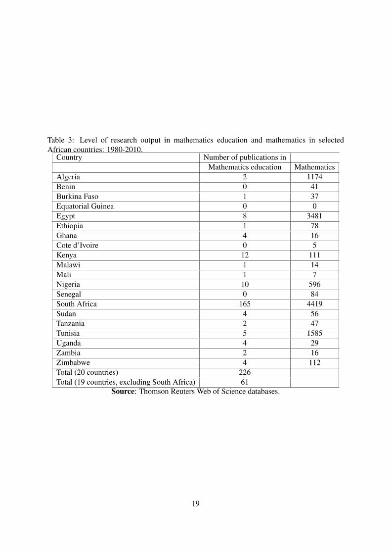
Table 3: Level of research output in mathematics education and mathematics in selectedAfrican countries: 1980-2010.

Country Number of publications inMathematics education Mathematics

Algeria 2 1174Benin 0 41Burkina Faso 1 37Equatorial Guinea 0 0Egypt 8 3481Ethiopia 1 78Ghana 4 16Cote d’Ivoire 0 5Kenya 12 111Malawi 1 14Mali 1 7Nigeria 10 596Senegal 0 84South Africa 165 4419Sudan 4 56Tanzania 2 47Tunisia 5 1585Uganda 4 29Zambia 2 16Zimbabwe 4 112Total (20 countries) 226Total (19 countries, excluding South Africa) 61

Source: Thomson Reuters Web of Science databases.

19

have little option but to allow recruitment of unqualified teachers. What kind of in-servicetraining is needed to bring them to qualified status?

4.2 Qualified teachers (pre-service programmes)

How are present mathematics teachers being prepared? Is their subject knowledge adequate?Is their pedagogical knowledge adequate? How closely should their mathematics curriculumbe aligned to the needs of the classroom (i.e. school mathematics curriculum)?

4.3 Qualified in-service teachers (continuous professional development)

Given the education and experience of qualified practicing teachers, what are appropriate pro-grammes for their continuous professional development? How often should in-service pro-grammes be offered? And where should they be offered? What modes of delivery are effective?

4.4 Mathematics curricula

The need for reform of mathematics curricula is predicated by, among other factors,

(a) Advances in mathematics (including, how mathematics interacts with other disciplines)

(b) Advances in mathematics education (e.g. learning theories)

(c) Advances in technology.

• To what extent are mathematics curricula in African education systems influenced bysuch factors?

• What is the role of the teacher in curriculum reform?

• What are the differences between the intended, implemented and achieved curriculum?

• Does the secondary school mathematics curriculum address the needs of all studentsadequately?

4.5 Gender

What explains the observation that in many African countries girls are less successful than boysin science-based subjects and are less ”keen on” them? How to identify and nurture girls thatdemonstrate ability in mathematics?

4.6 Language of instruction

I noted in section 2.1 above that the learning of mathematics requires a variety of linguisticskills that second-language learners may not have mastered. Furthermore, special problemsof reliability and validity arise in assessing the mathematics achievement of students from alanguage minority (Cuevas 1984).

• What is the student’s attitude towards the use of an official language as a medium ofinstruction in learning mathematics?

• What is the teacher’s attitude towards the use of an official language as a medium ofinstruction in teaching and learning mathematics?

20

• Are there significant differences in the mathematics performance of official languagelearners and proficient speakers of the official language?

It should be obvious from the foregoing that research problems in mathematics education aretypically multi-faceted and require an awareness of the complexity of the teaching and learningof mathematics and the surrounding social context. In view of the responsibility of depart-ments of mathematics for the promotion of mathematics in Africa (El Tom, 1984), it cannotbe overemphasized that mathematicians should strive to participate actively in this multidisci-plinary activity. Indeed, in the context of Africa, mathematics education is too important to beleft for non-mathematicians.

References[1] Adler, J. (1994). Mathematics teachers in the South African transition.Mathematics Edu-

cation Research Journal 6, 2, 101-112.

[2] Adler, J. (1998). A language for teaching dilemmas: Unlocking the complex multilingualsecondary mathematics classroom. For the Learning of Mathematics, 18, 24-33.

[3] Abedi, J. & Lord, C. (2001). The language factor in mathematics tests. Applied Measure-ment in Education, 14(3), 219-234

[4] Abedi, J. Courtney, M., Leon, S. Kao, J., and Azzam, T. (2006). English Language Learn-ers and Math Achievement: A Study of Opportunity to Learn and Language Accommo-dation (CSE Report 702, 2006). Los Angeles: University of California, Center for theStudy of Evaluation/National Center for Research on Evaluation, Standards, and StudentTesting.

[5] Cuevas, Gilberto J.(1984). Mathematics learning in English as a second language. Journalfor Research m Mathemarlcs, Vol. IS, No. 2, 134-144

[6] Developing Countries Strategies Group (2009). Mathematics in Africa: Challenges andOpportunities. A Report to the John Templeton Foundation. International MathematicalUnion. http://www.mathunion.org/publications/reports-recommendations.

[7] El Tom, M. E. A. (1984). The role of Third World university mathematics institutionsin promoting mathematics. Invited paper presented at the 5th International Congress onMathematical Education, Adelaide, Australia, 24-30 August 1984.

[8] El Tom, M. E. A. (2008). A new model for building capacity in mathematical research inAfrica. Open University, U. K., Working Paper Series No. 342. Gerdes, P. (2007). AfricanDoctorates in Mathematics: ACatalogue, Lulu.com

[9] Goe, L. (2007). The link between teacher quality and student outcomes:A research synthe-sis.Wahington, DC:National Comprehensive Center for Teacher Quality. Retrieved June21, 2012 from http://www.ncctq.org/publications/Link Between TQ and Student Out-comes.pdf

21

[10] Hanushek, E. A. (1995). Interpreting recent research on schooling in developing countries.The World Bank Research Observer, 10, 227-46.

[11] Hanushek, E. A., & Luque, J. A. (2003). Efficiency and equity in schools around theworld. Economics Of Education Review, 22, 481-502.

[12] Hanushek, Eric A., and Steven G. Rivkin (2006). ”Teacher Quality.” In Eric A. Hanushekand Finis Welch, eds., Handbook of the Economicsof Education. Amsterdam: North Hol-land.

[13] Harbison, R. W. & Hanushek, E. A. (1992). Educational performance of the poor: Lessonsfrom rural northeast Brazil. New York: Oxford University Press.

[14] Howie, Sarah J. (2003). Language and other background factors affecting secondarypupils’ performance in Mathematics in South Africa. African Journal of Research inMathematics Science and Technology Education, 7:1-20

[15] Moloi, M. Q. (undated). Mathematics achievement in South Africa: A comparison of theofficial curriculum with pupil performance in the SACMEQ II Project.

[16] Onderi, H. and Malala, G. (January 2011). A review on extent of sustainability of edu-cational projects: A case of strengthening of mathematics and science in secondary edu-cation (SMASSE) projects in Kenya. A review on extent of sustainability of educationalprojects: A case of strengthening of mathematics and science in secondary education(SMASSE) projects in Kenya. International Journal of Physical and Social Sciences, Vol.2, Issue 1 (Social Sciences http://www.ijmra.us).

[17] Philemon, C. (2010). Development of Science and Mathemat-ics. Paper presented at the Annual Meeting, Mathematical Associa-tion of Tanzania, September 2010 (retrieved on 10 May 2012 fromhttp://www.maths.udsm.ac.tz/mat/DEVELOPMENT%20OF%20SCIENCE%202010%20NEW.pdf)

[18] UNESCO (1953). The use of vernacular languages in educa-tion. Monograph on fundamental education VIII. Paris.UNESCO.(http://unesdoc.unesco.org/images/0000/000028/002897eb.pdf)

[19] UNESCO. 2006. Teachers and Educational Quality: Monitoring Global Needs for 2015.Montreal: UNESCO Institute for Statistics.

[20] Villegas-Reimers, E. (2003). Teacher professional development: An international reviewof the literature. Paris: UNESCO, International Institute for Educational Planning.. Re-trieved June 21, 2012 from http://unesdoc.unesco.org/images/0013/001330/133010e.pdf

[21] Zahiah Zakaria and Mohd Sallehhudin Abd Aziz (January 2011). Assessing Students Per-formance: The Second Language (English Language) Factor. International Journal ofEducational and Psychological Assessment January 2011, Vol. 6(2)

22

Mathematical Competitions for Gifted Students: Organization andTraining

by

Paul Vaderlind

Stockholm University, Sweden

What are the competitions?

In addition to regular competitions, problem-solving sessions during a limited time, like na-tional Olympiads or multiple-choice question exams, the World Federation of National Math-ematics Competitions has formally defined competitions as including enrichment courses andactivities in mathematics, mathematics clubs or ”circles”, mathematics days, mathematics camps,including live-in programs in which students solve open-ended or research-style problems overa period of days, and other similar activities. These activities all have in common the valuesof creativity, enrichment beyond the normal syllabus, opportunities for students to experienceproblem solving situations and provision of challenge for the student. Competitions give stu-dents the opportunity to be drawn by their own interest to experience some mathematics beyondtheir normal classroom experience.

Short history

Among all the methods for identifying gifted students, mathematical competitions probablyhas the longest and most successful history. The idea of competitions in mathematics goesback to the Hungarian Etvs/Kurschak Contest, 1894. First after forty years later came the St.Petersburg (1934) and Moscow (1935) Mathematical Olympiads. The competitions gaineda lot of popularity after the Second World War and resulted among other things in the firstInternational Mathematical Olympiads (1959). The success of the IMO was such that withina few years the number of participating countries grew from 7 to 20. Today more than 100countries from all continents participate in the IMO and those countries cover more than 85%of the population of our Planet. Many more countries have their national competitions but can’tafford sending a team to the IMO. This is a case with many developing countries.

The goals:

There are several goals of competitions in Mathematics.

1. An ultimate method for identifying gifted students,

2. To give students an opportunity to discover a latent talent in mathematics and providea stimulus for improving learning. Competitions provide opportunity for creativity andindependent thinking, as students often solve problems in unexpected and innovativeways.

3. To provide resources for the classroom activities: competitions are an important part oflearning mathematics and a fun activity for students of all ages. The success of competi-tions over the years, particularly the resurgence in the last 50 years, indicates that theseare events in which students enjoy mathematics. A long-term objective of the organizingcommittee of a mathematical contest should definitely be rising of the national educationlevel.

23

4. To highlight the importance of mathematics: competitions provide a focus on problemsolving, sometimes giving students an opportunity to be associated with a cutting edgearea of mathematics in which new methods may evolve and old methods be revived.

The practice.

Competitions come in a number of categories:

1. Local competitions on a school level, community level or town.

2. Provincial competitions within a country, which often are a part of more general nationalOlympiad.

3. National mathematical Olympiads.

4. Regional Olympiads, like Baltic Way Mathematical Contest, Asian-Pacific MathematicalOlympiad, Balkan Olympiad, Pan African Math Olympiad and so on.

5. International contests: IMO, Tournament of Towns, Kangaroo Mathematical Contest.

Other categories:

6. Competitions for girls only: China Girls’ Math Olympiad and European Girls’ MathOlympiad.

7. Team competitions: Baltic Way Team Competition and even contests involving wholeclasses, giving a very different feel to the competition.

8. Competitions for Primary schools and competitions for University students.

Competitions today

As we mentioned earlier, most countries have a permanent competitions activities althoughvery often those activities are limited to at most national level. Most of the time the reasonis lack of funds for travels and for training camps. However, the recent development showsthat more and more private companies (banks, investment corporations, telephone companiesand internet providers) discover a need of skilled, well-educated co-workers and are willing tosponsor different elite-search events, one of which is obviously mathematical competitions.

The questions offered at the competitions are most of the time non-standard problems beingnon-routine, provocative, fascinating, and challenging, often with elegant solutions. The topicsassume little prior knowledge beyond school curriculum and covers most of the school mathe-matics: geometry, trigonometry, algebra, inequalities, number theory and combinatorics.

Organizing a competition:

1. An organizing committee. Preferably consisting of a group of University teachers and agroup of Secondary school teachers.

24

2. Getting acquainted with the ”competitional mathematics”. This usually goes beyond thesecondary schools curriculum; demands some (accessible) knowledge and a good partof creativity. There are hundreds of books and numerous websites with different kindof competitions on different levels. Some help may be received from mathematicianscoming from countries with a long tradition in organizing olympiads.

3. Preparing a competition. Could be a competition covering only some schools of only onecity (the capital) or a number of cities and slowly, in the following years, extending it tothe whole country.

4. Getting in touch with at least one teacher of mathematics in each (if possible) school inthe country and prepare him/her for arranging a competition.

5. The first stage could be a multiple-choice questions. This is easily marked by the teacherand the results are then send to the national committee. In smaller countries, like Sweden,the papers are marked by the national committee during a weekend-long working session.

The best students may be then selected for the next stage. For example 20-50 students.It may be a provincional competition or already a national final. It is important howeverthat at this stage the questions demand a full solution, not a multiple-choices alternatives.

6. Training of the most successful and promising students for further, international compe-titions.

7. Participating in an International regional competition, for example PAMO, or creatingsmaller events, like East African Mathematical Challenge. It doesn’t have to involvetravels (the students, up to 10 from each country, can work in their schools, but the pa-pers may be marked by one ”hosting country”, which may vary from year to year.

This year PAMO will take place September 8-16 this year in Tunisia. The country reg-istered that far are Mali, Tunisia, Burkina Faso, Algeria, Tanzania, Kenya, Gambia, Cted’Ivoire, Nigeria, Egypt and South Africa.

wwww.pamo− official.org

8. IMO - the queen of all competitions. In the latest one, in Argentina, July 2012, par-ticipated 100 countries from all over the world, but only six from Africa (Uganda, IvoryCoast, South Africa, Nigeria, Tunisia and Morocco). Next IMO will take place in Colom-bia (2013) and then in Cape Town (2014), for the first time on the African soil.

www.imo− official.org

www.artofproblemsolving.com

25

Estimation of IBNR Claims Reserves Using Linear Modelsby

Patrick G. O. Weke

School of Mathematics, University of Nairobi, Kenya

Abstract

Stochastic models for triangular data are derived and applied to claims reserving data.The standard actuarial technique, the chain ladder technique is given a sound statisticalfoundation and considered as a linear model. The chain ladder technique and the two-way analysis of variance are employed for purposes of estimating and predicting the IBNRclaims reserves.

1. IntroductionIf claims runoff triangles are to be analysed statistically, as a data analysis exercise, it is desir-able to express them as linear models. If the claims are analysed using a model for each row,then it may be straightforward to write down a linear model. The use of linear models to anal-yse the data by row can give useful insights into the nature of the data, but it is the linear modelwhich is close to the chain ladder technique that is of greatest interest to actuaries. This linearmodel, whose connection with the chain ladder technique was first identified by Kremer[4] isdescribed in sections 3 and 4.

The data are assumed to be lognormally distributed and is first logged before a linear model isapplied. The transformation from the raw data to the logged data is, obviously, straightforward,but the reverse transformation, once the analysis has been carried out, is not simple. This isdealt with in section 5. The process is represented in Figure 1.

Figure 1:

Prediction from linear models when the data are lognormally distributed was first considered byFinney [3]. Finney considered a sample of independently, identically distributed data, and thetheory was generalized to a sample of independently, but not necessarily identically distributeddata by Bradu and Mundlak [2]. Subsequent papers by Renshaw [5], Verrall [6], and Weke [8]

26

have considered the properties of the estimators in more detail. The techniques outlined in thispaper have been implemented in GLIM (Baker and Nelder [1] and the results shown.

2. Linear ModelsThe linear model to be considered is

y = Xβ + ε (2.1)

where y is a data vector of length n, β is an n × p design matrix and ε is an error vector oflength n. The error vector ε is assumed to have mean zero and variance-covariance matrix Σ.

The minimum variance linear unbiased estimators of the parameters, β, are the weighted least-squares estimators, β, where

β =(X ′Σ−1X

)−1X ′Σ−1y (2.2)

If the errors, ε, are assumed to be jointly normally distributed, then the estimators, β, arealso the maximum likelihood estimators. Since a logarithmic transformation will be appliedto the data, the reverse transformation to estimate actual claims will depend on the estimationmethod being used. One estimator can be obtained by simply substituting the estimators intothe equations. This is used in the lemmas which show the similarity between the chain laddertechnique and a certain linear model. However, these estimators, and indeed the maximumlikelihood estimators, are biased, and it may be better to use unbiased estimators. If the errorsare assumed to be uncorrelated with equal variance then equation (2.1) simplifies to

β = (X ′X)−1X ′y (2.3)

which is a form which will also be used.

The distributional properties of the maximum likelihood estimators, β, are well-known. As-suming that the errors are independently, identically distributed with variance σ3,

β ∼ N(β, σ2(X ′X)−1

)(2.4)

3. The Chain Ladder Technique as a Linear ModelKremer [4] showed that the chain ladder technique is very similar to a two-way analysis ofvariance and investigated the properties of the estimators. This section describes the connectionbetween the actuarial chain ladder technique and the statistical analysis of variance method.Assuming a triangular data set (without loss of generality) the cumulative claims data, to whichthe chain ladder technique is applied, are

Cij = i = 1 . . . , t; j = 1 . . . , t− i+ 1 (3.1)

The differenced data, to which the analysis of variance model is applied, are

Zij : i = 1, . . . , t; j = 1 . . . , t− i+ 1 (3.2)

whereZij = Cij − Ci,j−1, j ≥ 2Zi,1 = Ci1

27

The chain ladder technique is based on the model

E[Cij] = λjCi,j−1; j = 2, . . . , t. (3.3)

The parameter λj is estimated by λj , where

λj =

i−j+1∑i=1

Cij

i−j+1∑i=1

Ci,j−1

(3.4)

The expected ultimate loss, E[Cij], is estimated by multiplying the latest loss, Ci,i−j+1, by theappropriate estimated λ-values:

estimate of E[Cij] =

(t∏

j=t−i+2

λj

)Ci,i−j+1 (3.5)

The chain ladder technique produces forecasts which have a row effect and a column effect.The column effect is obviously due to the parameters λj : j = 2, . . . , t. There is also a roweffect since the estimates for each row depend not only on the parameters λj : j = 2, . . . , t,but also on the row being considered. The latest cumulative claims, Ci,t−i+1, can be consideredas the row effect. This leads to consideration of other models which have row and columneffects, in particular the two-way analysis of variance model. The connection is first madewith a multiplicative model (see [7]). This uses the non-cumulative data, Zij , and models themaccording to:

EbZijc = UiSj (3.6)

where Ui is a parameter for row i, and Sj is a parameter for row j.

A multiplicative error structure is assumed and also

t∑j=1

Sj = 1 (3.7)

In this model, Sj is the expected proportion of ultimate claims which occur in the jth develop-ment year; and Ui is the expected total ultimate claim amount for business year i (neglectingany tail factor). The estimates of Ui will be compared with the estimates of E[Cit] in equation(3.5) and Sj and λj will be related to each other.

The analysis of variance estimators are based on the model (3.6):

EbZijc = UiSj

and the chain ladder technique is based on the model (3.3):

E[Cij] = λjCi,j−1; j = 2, . . . , t.

In terms of the models, ignoring for the moment the estimation of the parameters, this simplyrepresents a reparameterisation.

28

Under the chain ladder model, the expected claim total for business year is

t∏j=t−i+2

λjCi,t−i+1 (3.8)

and the expected claim amount in development year t− i+ 2 is

λt−i+2Ci,t−i+1 − Ci,t−i+1 (3.9)

The equivalent quantities under the multiplicative model (3.6) are

Ui (3.10)

and UiSt−i+2 (3.11)

Equating (3.8) and (3.9) with (3.10) and (3.11), respectively, gives

St−i+2 =λt−i+2 − 1

t∏j=t−i+2

λj

The expected claim amount for development year t− i+ 3 under each model is

λt−i+3λt−i+2λt−i+1 − λt−1+2Ci, t− i+ 1 (3.12)

andUiSt−i+3 (3.13)

which gives

St−i+3 =λt−i+3 − 1

t∏j=t−i+3

λj

In general, the expected proportion of ultimate claims can be written in the form

Sj =λj − 1t∏l=j

λl

(3.14)

Considering year of business t, the expected total claim amount under each model is[t∏

j=2

λj

]Ct1

and Ut.

The claim amount in development year 1, Ct1, is modeled by UtS1, and so it can be seen that

S1 =1t∏l=j

λl

(3.15)

29

To summarize, the chain ladder model (3.3) is equivalent to the multiplicative model given byequation (3.6) with the following relationships between the parameters:

S1 =

(t∏l=2

λl

)−1

Sj =

(t∏l=2

λl

)−1

(λj − 1)

Ui = E(Cit).

Equations (3.4) and (3.5) give the estimates of λj : j = 2, . . . , t and E(Cit). Estimators ofSi : i = 2, . . . , t and Uj : j = 2, . . . , t can be obtained by applying a linear model to thelogged incremental claims data. Taking logs of both sides of equation (3.6), and assuming thatthe incremental claims are positive, results into

E(Yij) = µ+ αi + βj (3.16)

where Yij = logZij denotes the cumulative claims in development year j in respect of accidentyear i, and the errors now have an additive structure and are assumed to have mean zero. Theerrors will be assumed to be identically distributed with variance σ2 , although this distribu-tional assumption can be relaxed. Kremer [4] defines as the mean of the logUis and logSjs, sothat the restriction

t∑i=1

αi =t∑

j=1

βj = 0

is imposed.

An alternative assumption is that α1 = β1 = 0 . In this case

αi = logUi − logU1 (3.17)βj = logSj − logS1 (3.18)µ = logU1 + logS1 (3.19)

The latter set of assumptions are more appropriate for the more sophisticated techniques. How-ever, prediction and estimation of the claims is unaffected by the choice of the assumptions.

The assumption that error terms, εij , are independently, identically distributed with varianceσ2 will be used, so that the estimators are given by equation (2.3) Now equation (3.16) can bewritten in the form of equation (2.1). Suppose, for example, there are three years of data then

y11

y12

y21

y13

y22

y31

=

1 0 0 0 01 0 0 1 01 1 0 0 01 0 0 0 11 1 0 1 01 0 1 0 0

µα2

α3

β2

β3

+

ε11

ε12

ε21

ε13

ε22

ε31

(3.20)

clearly gives the form of the parameter vector and the design matrix.

The following lemma, due to Kremer [4], gives the normal equations for the chain ladder linearmodel.

30

Lemma 3.1 For n years data, the best linear unbiased estimators of µ, αi, βj are the solutionsof

αi =1

t− i+ 1

∑(Yij −

1

t− j + 1

t−j+1∑l=1

(Y1j − αl)

); i = 2, . . . , t (3.21)

βj =1

t− j + 1

∑(Yij −

1

t− j + 1

t−j+1∑l=1

(Y1j − βl)

); j = 2, . . . , t (3.22)

µ =1

t(t+ 1)

t∑i=1

t−i+1∑j=1

(Yij − αi − βj). (3.23)

Proof:The normal equations, (2.3), are

(t− i+ 1)µ+ (t− i+ 1)αi +t−i+1∑j=2

βj =t−u+1∑j=1

Yij; i = 2, . . . , t (3.24)

(t− i+ 1)µ+t−i+1∑j=2

αi + (t− j + 1)βj =t−u+1∑j=1

Yij; i = 2, . . . , t (3.25)

t(t+ 1)

2µ+

t∑i=2

(t− i+ 1)αi +t∑

j=2

(t− j + 1)βj =t∑i=1

t−i+1∑j=1

Yij (3.26)

Noting that α1 = β1 = 0 , equations (3.26) and (3.23) are equivalent. Also equations (3.24)and (3.25) can be written as

αi =1

t− i+ 1

t−i+1∑j=1

(Yij − βj)− µ (3.27)

βi =1

t− i+ 1

t−i+1∑i=1

(Yij − βj)− µ (3.28)

Substituting equation (3.27) into equation (3.28) and vice versa gives equations (3.21) and(3.22).

4. Relationship between the Estimators of the Linear Model and the ChainLadder ModelThe previous section derived the relationship between the parameters of the multiplicativemodel and the chain ladder technique. The parameters are estimated in different ways ac-cording to which method is used, and this section is devoted to examining the relationshipsbetween the estimators of the parameters.

This section contains two lemmas. The first deals with the estimation of Sj and Ui - the param-eters of the multiplicative model using the chain ladder technique. The second lemma derivesthe estimators of Sj and Ui using the two-way analysis of variance model. The two sets of es-timators are then shown to be similar. Thus, it will be shown that the chain ladder method will

31

produce results which are similar to those produced by the analysis of variance method. Thelatter has been studied in great depth in statistical literature and the method has the advantageof a great deal of theoretical background. The theory of analysis of variance will be applied toinsurance data, bearing in mind that the main method in use in the industry is the chain laddermethod.

Lemma 4.2 If


λl

; j = 2, . . . , t (4.1)

and λj is estimated by λj , where

λj =

t−j+1∑i=1

Cij

t−j+1∑i=1

Cij−1

(4.2)

then the estimators of Sj , Sj , satisfy the relationship

Sj =

t−j+1∑i=1

Y ij

t−j+1∑i=1

Ci,t−i+1

/(1−

t∑l=t−i+2

Sl

) (4.3)

Also, the estimate of Ui is Ui, where

Ui =

t−i+1∑j=1

Zij

t−i+1∑j=1

Sj

. (4.4)

Proof:Equations (4.1) and (4.2) imply that


λl

=

t−j+1∑i=1

Cij −t−j+1∑i=1

Cij−1

t−j+1∑i=1

Cij

t∏l=1

λl

(4.5)

Now, it can be shown by induction that (see [4])

t−j+1∑i=1

Cij =

t−j+1∑i=1

Ci,t−i+1

/t−i+1∏l=j+1

λl (4.6)

32

Substituting equation (4.6) into equation (4.5) gives

Sj =

t−j+1∑i=1

Zij(t−j+1∑i=1

Ci,t−i+1

/t−i+1∏l=j+1

λl

)t∏

l=j+1

λl

=

t−j+1∑i=1

Zij

t−j+1∑i=1

Ci,t−i+1

t∏l=t−i+2

λl

(4.7)

It can also be shown by induction that[t∏l=k

λl

]−1

= 1−t∑l=k

Sl.

This is true for k = 2 by virtue of (3.15) and the relationship

1−t∑l=2

Sl = S1.

Suppose it is true for k . Then for k + 1:

1−t∑

l=k+1

Sl = 1−t∑l=k

Sl + Sk

=

[t∏l=k

λl

]−1

+λk − 1t∏l=k

λl

=

[t∏

l=k+1

λl

]−1

(4.8)

Hence, by induction, the result holds. Substituting this result into (4.7) gives

Sj =

t−j+1∑i=1

Zij

t−j+1∑i=1

Ci,t−i+1

/(1−

t∑l=t−i+2

Sl

) (4.9)

as required.

Now, since Ci,t−i+1 =t−i+1∑j=1

Zij

andt∏

j=t−1+2

λj =

(1−

t∑j=t−i+2

Sj

)−1

the estimate of total expected outstanding claims for

row i,

Ci,t−i+1

t∏j=t−i+2

λj

33

can be written as

t−i+1∑j=1

Zij

1−t∑

j=t−i+2

Sj

.

This can be written ast−i+1∑j=1

Zij

/t−i+1∑j=1

Sj (4.10)

since 1−t∑

j=t−i+2

Sj = 1−t−i+1∑j=i

Sj .

Lemma 4.3 Using the estimation method of Lemma 3.1, an estimate of total expected claimsfor accident year i, Ui, is given by

Ui =

[t−i+1∏j=1

Zijwj

] 1t−i+1

·t−i+1∑j=1

wj (4.11)

where

wj =

[t−i+1∏j=1

Zij

] 1t−j+1

t−j+1∏i=1

(t−i+1∏l=1

Zil

) 1t−i+1

/(t−i+1∏l=

wl

) 1t−i+1

1

t−j+1

(4.12)

Further,

Ui =

[t−i+1∏j=1

Zij

] 1t−i+1

[t−i+1∏j=1

Sj

] 1t−i+1

(4.13)

This lemma can be used to show that the estimates of expected total outstanding claims for eachrow have similar forms using each method, and can be expected to behave in similar ways. Theestimate of Ui is obtained by “hatting” the parameters in the identity

Ui = eαieµt∑

j=1

eβj

which is derived in the proof of this lemma. The resulting estimate of Ui is not the maxi-mum likelihood estimate, neither is it unbiased, but it does serve the purpose of illustrating thesimilarity between the chain ladder technique and the two-way analysis of variance.

34

Proof: The equations (3.17) to (3.19) imply that

eαi =UiU1

(4.14)

eβj =SjS1

(4.15)

andeµ = U1S1. (4.16)

Sincet∑

j=1

Sj = 1, S1 =

(t∑

j=1

eβj

)−1

.

This, together with equations (4.14) and (4.16) gives

Ui = eαieµt∑

j=1

eβj (4.17)

Now let wj = eβj ; then equation (3.22) is equivalent to equation (4.12).

The best linear unbiased estimate of αi + µ is obtained from equation (3.27). Substituting theestimates of αi + µ and βj into equation (4.17) gives the estimate of Ui in equation (4.11).

Now, equation (4.15) implies that Sj = wj

/t∑l=1

wl and so equations (4.11) and (4.12) can be

written as

Ui =

[t−i+1∏j=1

Zij

] 1t−i+1

[t−i+1∏j=1

Zj

] 1t−i+1

and

Sj =

[t−i+1∏j=1

Zij

] 1t−j+1

t−j+1∏i=1

(t−i+1∏l=1

Zil

) 1t−i+1

/(t−i+1∏l=

Sl

) 1t−i+1

1

t−j+1

(4.18)

Now, if all the geometric means are replaced by arithmetic means in equation (4.18), the re-currence relation for the estimators of becomes the same as that in Lemma 4.2. Similarly theestimators of Ui are equivalent if geometric means are replaced by arithmetic means. Thusthe two estimation methods, the chain ladder method and the linear model, will produce sim-ilar results. The structure of the models is identical and the only difference is the estimationtechnique. It can be argued that the linear model estimates are best in a statistical sense, but it

35

should be emphasized that in using the linear model instead of the crude chain ladder technique,there are no radical changes.

5. Unbiased Estimation of Reserves and Variances of ReservesIt has been shown that the chain ladder can be considered as a two-way analysis of variance.This linear model, and other linear models, can be used effectively for analyzing claims dataand producing estimates of expected total outstanding claims for each year of business. Themethods have in common the assumption that the data is lognormally distributed, and the linearmodels are therefore applied to the logged incremental claims rather than the raw incrementalclaims data. The problem therefore arises of reversing the log transformation to produce esti-mates on the original scale. It is this problem which is addressed in this section; in particular theunbiasedness of the estimates is considered. It is important that estimates should be unbiasedin order that they are aiming at the correct target and do not yield values which consistentlyunder- or over-estimate. It is also important to consider unbiased estimation of the standarderror of the estimates of expected total outstanding claims, in order that some measure of theorder of the errors can be attached to the predictions. The procedure for analyzing claims datausing loglinear models is illustrated by Figure 1.

The final stage in this procedure reversing the log transformation is considered here andunbiased estimates of total outstanding claims are derived. Unbiased estimates of the variancesof these estimates are derived. The theory is applied to claims data (obtained from [7]) using theanalysis of variance linear model and the unbiased estimates compared with some alternatives.In order to make the analysis more easily assimilable, a sample of independently, identicallydistributed observations is considered first. The theory is then extended to the more generalcase of independent, but not necessarily identically distributed observations. It is the moregeneral theory which is applicable to claims data.

5.1 Unbiased Estimates of Total Outstanding Claims

The purpose of the analysis of the claims data is to produce estimates of the expected totaloutstanding claims, Ri, for each year of business, and the total outstanding claims, R, for thewhole triangle.

An unbiased estimate of Ri is Ri, where

Ri =t∑

j=t−i+2

θij. (5.1)

andθij = exp(X ijβ + σ2) (5.2)

is the maximum likelihood estimate of the expected value of the lognormally distributed data,θij , which is related to the mean and variance of the normally distributed data by

θij = exp(X ijβ + σ2/2).

The variance of Ri can be calculated from

Var(Ri) = Var

[t∑

j=t−i+2

θij

]=

t∑j=t−i+2

[Var(θij) + 2

t∑k=j+1

Cov(θij, θik)

]. (5.3)

36

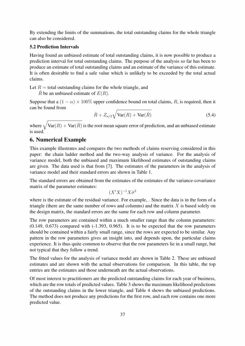
By extending the limits of the summations, the total outstanding claims for the whole trianglecan also be considered.

5.2 Prediction Intervals

Having found an unbiased estimate of total outstanding claims, it is now possible to produce aprediction interval for total outstanding claims. The purpose of the analysis so far has been toproduce an estimate of total outstanding claims and an estimate of the variance of this estimate.It is often desirable to find a safe value which is unlikely to be exceeded by the total actualclaims.

Let R = total outstanding claims for the whole triangle, andR be an unbiased estimate of E(R).

Suppose that a (1− α)× 100% upper confidence bound on total claims, R, is required, then itcan be found from

R + Za/2

√Var(R) + Var(R) (5.4)

where√

Var(R) + Var(R) is the root mean square error of prediction, and an unbiased estimateis used.

6. Numerical ExampleThis example illustrates and compares the two methods of claims reserving considered in thispaper: the chain ladder method and the two-way analysis of variance. For the analysis ofvariance model, both the unbiased and maximum likelihood estimates of outstanding claimsare given. The data used is that from [7]. The estimates of the parameters in the analysis ofvariance model and their standard errors are shown in Table 1.

The standard errors are obtained from the estimates of the estimates of the variance-covariancematrix of the parameter estimates:

(X ′X)−1Xσ2

where is the estimate of the residual variance. For example, . Since the data is in the form of atriangle (there are the same number of rows and columns) and the matrix X is based solely onthe design matrix, the standard errors are the same for each row and column parameter.

The row parameters are contained within a much smaller range than the column parameters:(0.149, 0.673) compared with (-1.393, 0.965). It is to be expected that the row parametersshould be contained within a fairly small range, since the rows are expected to be similar. Anypattern in the row parameters gives an insight into, and depends upon, the particular claimsexperience. It is thus quite common to observe that the row parameters lie in a small range, butnot typical that they follow a trend.

The fitted values for the analysis of variance model are shown in Table 2. These are unbiasedestimates and are shown with the actual observations for comparison. In this table, the topentries are the estimates and those underneath are the actual observations.

Of most interest to practitioners are the predicted outstanding claims for each year of business,which are the row totals of predicted values. Table 3 shows the maximum likelihood predictionsof the outstanding claims in the lower triangle, and Table 4 shows the unbiased predictions.The method does not produce any predictions for the first row, and each row contains one morepredicted value.

37

Table 3: Maximum likelihood predictions of outstanding claims101269

357398 93599

217465 319835 83761

335047 243001 357392 93597

386433 345088 250283 368102 96402

617309 418743 373941 271209 398880 104462

1206369 674243 457364 408430 296223 435668 114097

1026594 1053911 589034 399564 356813 258787 380610 99678

888831 913640 937951 524224 355600 317554 230313 338732 88710

Table 4: Unbiased predictions of outstanding claims96238

350362 88841

215218 313105 79394

332848 240075 349268 88564

384305 342028 246696 358900 91006

613257 415031 369373 266419 387593 98281

1193906 666126 450811 401216 289387 421005 106752

1006382 1031734 575643 389575 346716 250077 363813 92248

844677 867203 889047 496032 335695 298762 215487 313486 79483

38

Table 1: Estimates of the row and column and their standard errorsEstimate Standard Error

Overall mean 6.106 0.165Row parameters 0.194 0.161

0.149 0.1680.153 0.1760.299 0.1860.412 0.1980.508 0.2140.673 0.2390.495 0.2810.602 0.379

Column parameters 0.911 0.1610.939 0.1680.965 0.1760.383 0.186-0.005 0.198-0.118 0.214-0.439 0.239-0.054 0.281-1.393 0.379

It can be seen that the maximum likelihood estimates are all higher than the unbiased estimates,as was to be expected.

The total predicted outstanding claims for each year of business (the row totals of the pre-dicted outstanding claims) are shown in Table 5. There are three estimates given, the maximumlikelihood and unbiased estimates from the analysis of variance model, and the chain ladderestimate.

It can be seen that the maximum likelihood estimates differ most significantly from the unbi-ased estimates in the early and late rows. The estimates for the middle rows are the closesttogether, which is where the number of observations are used in the estimation is the greatest.The maximum likelihood estimate is asymptotically unbiased, and the greater the number ofobservations used to estimate the parameters, the closer are the two. The chain ladder estimatesare sometimes higher and sometimes lower than the analysis of variance estimates. There isnothing significant that can be inferred from the differences. This confirms that the crude chainladder method is a reasonable rough and ready method for calculating outstanding claims, al-though the more proper method, statistically, is the analysis of variance method (using unbiasedestimation).

The total predicted outstanding claims are:

Analysis of Maximum Likelihood 18186154Variance Unbiased 17652064

Chain Ladder 18619916

39

Table 2: Fitted values and the actual observations

286170 711785 731359 750301 418911 283724 252756 182559 266237 67948357848 766940 610542 482940 527326 574398 146342 139950 227229 67948

410587 1021245 1049329 1076506 601040 407078 362646 261930 381987352118 884021 933894 1183289 445745 320996 527804 266172 425046

379337 943516 969461 994572 555294 376094 335044 241994290507 1001799 926219 1016654 750816 146923 495992 280405

339233 843767 866971 889425 496588 336334 299624310608 1108250 776189 1562400 272482 352053 206286

378676 941872 967773 992840 554327 375439443160 693190 991983 769488 504851 470639

389421 968599 995234 1021012 570056396132 937085 847498 805037 705960

420963 1047052 1075844 1103710440832 847631 1131398 1063269

457887 1138894 1170213359480 1061648 1443370

396651 986582376686 986608

344014344014

Table 6 below shows the unbiased estimates of the total outstanding claims for each year ofbusiness, the standard errors of these estimates and the root mean square error of prediction.This table can be used in setting safe reserves, and gives an idea of the likely variation ofoutstanding claims.

The unbiased estimate of total outstanding claims is 17652064 and the root mean square errorof prediction is 2759258. Thus a 95% upper bound on total outstanding claims is

17652064 + 1.645× 2759258 = 22191043.

This is a safe reserve for this triangle according to the chain ladder linear model using unbiasedestimation.

40

Table 5: Total predicted outstanding claimsAnalysis of Variance

Row Maximum Likelihood Unbiased Chain Ladder2 101269 96238 946303 450997 439203 4646684 621061 607717 7021015 1029037 1010755 9655766 1446307 1422934 14122027 2184544 2149953 21760898 3592393 4520202 38971429 4164990 4056189 4289473

10 4595556 4339873 4618035

Table 6: Unbiased estimates, standard errors and root MSE for each yearUnbiased Standard Mean Square ErrorEstimate Error of prediction96238 35105 47202439203 108804 163217607717 127616 1828471010755 195739 2692241422934 273082 3575932149953 429669 5385333529202 775256 9428514056189 1052049 11970094339873 1534943 1631306

41

7. ConclusionIn conclusion, some practical aspects of claims reserving have been considered. These are thestability of the estimation and predictions, the use of the predictions, their standard errors andthe safe reserves in practice. The connection between the linear model and the chain laddertechnique has been outlined.

References[1] Baker, R. J. & Nelder, J. A. (1978). The GLIM System: Release 3, Numerical Algorithms

Group, Oxford.

[2] Bradu, D. & Mundlak, Y. (1970). Estimation in Lognormal Linear Models. JASA, Vol. 6,198-211.

[3] Finney, D. J. (1942). On the Distribution of a Variate whose Logarithm is Normally Dis-tributed. JRSS Suppl., 7, 155-161.

[4] Kremer, E. (1982). IBNR Claims and the Two-Way Model of ANOVA. Scand. Act. J.,Vol. 1, 47-55.

[5] Renshaw, A. E. (1989). Chain Ladder and Interactive Modelling: Claims Reserving andGLIM. Journal of the Institute of Actuaries, Vol. 116, Part 3, 559-587.

[6] Verrall, R. J. (1989). A State Space Representation of the Chain Linear Model. Journal ofthe Institute of Actuaries, Vol. 116, Part 3, 589-609.

[7] Weke, P. G. O. (2003). Estimating IBNR Claims Reserves using Gamma Model andGLIM. The Nigerian Journal of Risk and Insurance, Vol. 4, No. 1, 1-11.

[8] Weke, P. G. O. & Mureithi, A. T. (2006). Deterministic Claims Reserving in Short-TermInsurance Contracts. The East African Journal of Statistics, Vol. 1, No. 2, 198-213.

42

Heat Transfer Analysis of a Convecting and Radiating Two Step ReactiveSlab

by

O. D. Makinde

Institute for Advanced Research in Mathematical Modeling and Computation,Cape Peninsula

University of Technology, P.O. Box 1906, Bellville 7535, South Africa

Abstract

This paper examined the heat transfer characteristic of a steady state convecting and ra-diating two step exothermic reactive slab of combustible materials, taking the diffusion ofthe reactant into account and assuming a variable (temperature dependent) pre-exponentialfactor. The nonlinear differential equation governing the reaction-diffusion problem is ob-tained and tackled numerically using Runge-Kutta- Fehlberg method with shooting tech-nique. The effects of various embedded thermophysical parameters on the temperaturefield are presented graphically and discussed quantitatively.

Keywords: Rectangular slab; Two steps exothermic reaction; Convective heat loss,Radiative heat loss; Hermite-Pad approximants

1. IntroductionHeat transfer in a reactive slab of combustible materials due to exothermic chemical reactionplays a significant role in improving the design and operation of many industrial and engineer-ing devices and find applications in power production, jet and rocket propulsion, fire preventionand safety, pollution control, material processing industries and so on [1–3]. For instance, solidpropellants used in rocket vehicles are capable of experiencing exothermic reactions withoutthe addition of any other reactants. The theory of heat transfer in reactive materials has longbeen a fundamental topic in the field of combustion. The chemical reaction may be modelledby considering either a single step or multi step reaction kinetics. For instance catalytic con-verter used in an automobile’s exhaust system provides a platform for a two step exothermicchemical reaction where unburned hydrocarbons completely combust. This helps to reduce theemissions of toxic car pollutant such as carbon monoxide (CO) into the environment. The mainchemical reaction schemes in an autocatalytic converter are [4],

2NO =⇒ N2 +O2 or 2NO2 =⇒ N2 + 2O2 (Reduction process)2CO +O2 =⇒ 2CO2 (Oxidation process).

Similarly, the combustion taking place within k-fluid is treated as a two step irreversible chem-ical reaction of methane oxidation as follows [5]:

CH4 + 1.5(O2 + 3.76N2) = CO + 2H2O + 5.6N2

CO + 0.5(O2 + 3.76N2) = CO2 + 1.88N2.

The vast majority of studies on chemically reactive materials have been concerned with homo-geneous boundary conditions ranging from the infinite Biot number case [6] (Frank-Kamenetskii

43

conditions) to a range of Biot numbers [7] (Semenov conditions). Mathematical models of theproblem relating to exothermic reaction in a reactive slab may be extremely stiff owing to thetemperature dependence of the chemical reactions. Moreover, the differential equation for thetemperature distribution in a convectiveradiative reactive slab with temperature dependent pre-exponential factor is highly nonlinear and does not admit an exact analytical solution [8]. Con-sequently, the equation has been solved either numerically or using a variety of approximatesemi-analytical methods [9–11]. The preceding literature clearly shows the work on reactingslab has been confined to convective surface heat loss. No attempt has been made to studythe combined effects of convective and radiative heat losses at the slab surface despite its rele-vance in various technological applications such as aerothermodynamic heating of spaceshipsand satellites, nuclear reactor thermohydraulics and glass manufacturing. Thermal radiation ischaracteristic of any material system at temperatures above the absolute zero and becomes animportant form of heat transfer in devices that operate at high-temperatures. Radiation is thedominant form of heat transfer in applications such as furnaces, boilers, and other combustionsystems.

The present investigation aims to extend the recent work of Makinde [11, 12] to include com-bined effects of convective and radiative heat losses on a slab of combustible material withinternal heat generation due to a two step exothermic reaction. It is hoped that the results ob-tained will not only provide useful information for applications, but also serve as a complementto the previous studies.

2. Mathematical ModelLet us consider the dynamical thermal behaviour of a rectangular slab of combustible materi-als with internal heat generation due to a two step exothermic chemical reaction, taking intoaccount the diffusion of the reactant and the temperature dependent variable pre-exponentialfactor. The geometry of the problem is depicted in Fig. 1. It is assumed that the slab surface issubjected to both convective and radiative heat losses to the environment.

Figure 1: Sketch of the physical model.

The one-dimensional heat balance equation in the original variables together with the boundary

44

conditions can be written as [1, 3, 10, 11]:

kd2T

dy2+ Q1C1A1

(KT

νg

)meE1RT +Q2C2A2

(KT

νg

)meE2RT − εσ[T − T 4

∞] = 0, (2.1)

kdT

dy(0) = h1[T (0)− T∞], k

dT

dy= −h2[T (a)− T∞], (2.2)

where T is the absolute temperature, T∞ is the ambient temperature, h1 is convective the heattransfer coefficient at the lower surface, h2 is convective the heat transfer coefficient at theupper surface, k is the thermal conductivity of the material, ε is the slab surface emissivity, σ isthe StefanBoltzmann constant; Q1 is the first step heat of reaction, Q2 is the second step heat ofreaction, A1 is the first step reaction rate constant, A2 is the second step reaction rate constant,E1 is the first step reaction activation energy, E2 is the second step reaction activation energy,ρ is the density, R is the universal gas constant, C1 is the first step reactant species initialconcentration, C2 is the second step reactant species initial concentration, g is the Plancksnumber, K is the Boltzmanns constant, ν is vibration frequency, a is the slab half width, y isdistance measured in the normal direction to the plane cp is the specific heat at constant pressureand m is the numerical exponent such that m = −2, 0, 1

2 represent numerical exponent

for Sensitised, Arrhenius and Bimolecular kinetics respectively [1, 3, 9–11]. The followingdimensionless variables are introduced into Eqs. (2.1) - (2.3):

θ =E1(T − T∞)

RT 2∞

, γ =RT∞E1

, y =y

a, β =

Q2C2A2

Q1C1A1

eE1−E2RT∞ , r =

E2

E1

, (2.3)

Bi1 =ha

k, Bi2 =

ha

k, λ =

E1a2Q1C1A1

kRT 2∞

[KT∞νg

]me−

E1RT∞ , Nr =

εσaE1T3∞

kR,

and we obtain the dimensionless governing equation as

d2θ

dy2+ λ(1 + γθ)m

[e(

θ1+γθ ) + βe(

rθ1+γθ )

]−Nr

[(γθ + 1)4 − 1

]= 0 (2.4)

withdθ

dy(0) = Bi1θ(0),

dθ

dy(1) = −Bi2θ(1) (2.5)

where λ, γ, β, r,Nr,Bi1, Bi2, represent the Frank-Kamenetskii parameter, activation energyparameter, two step exothermic reaction parameter, activation energy ratio parameter, ther-mal radiation parameter, the Biot numbers for the slab lower and upper surfaces respectively.Equations (2.4) and (2.5) represent a nonlinear boundary value problem. This nonlinear na-ture precludes its exact solution, using Runge-Kutta-Fehlberg method with shooting technique,the problem is tackled numerically and the slab surface heat transfer rate Nu = −θ′(1) isdetermined.

3. Results and DiscussionWe have assigned numerical values to the parameters encountered in the problem in order toget a clear insight into the thermal development in the system. It is very important to note thatβ = 0 corresponds to a one step chemical reaction case; an increase in the value β > 0 signifiesan increase in the two step chemical reaction activities in the system.

45

Table 1: Computation showing the critical values of the reaction rate parameter, Bi1 = 1.Nr Bi2 β r m γ Nu λc1 1 0.1 0.1 0.5 0.1 1.0825 0.81795 1 0.1 0.1 0.5 0.1 1.1927 1.546810 1 0.1 0.1 0.5 0.1 1.2486 2.46321 5 0.1 0.1 0.5 0.1 2.3721 1.31291 100 0.1 0.1 0.5 0.1 3.0569 1.66141 1 0 0.1 0.5 0.1 1.0358 0.84761 1 1 0.1 0.5 0.1 1.3910 0.64151 1 0.1 1 0.5 0.1 1.0421 0.77061 1 0.1 2 0.5 0.1 0.8331 0.66691 1 0.1 0.1 0 0.1 1.1662 0.87131 1 0.1 0.1 −2 0.1 1.7903 1.19411 1 0.1 0.1 0.5 0.2 4.2475 1.35311 1 0.1 0.1 0.5 0.4 1.4386 2.6350

Table 1, illustrates the variation in the values of thermal criticality conditions (λc) for differ-ent combination of embedded parameters. The magnitude of thermal criticality decreases withincreasing values of two step reaction rate parameter β > 0 and the activation energies ratio pa-rameter r > 0. This implies that thermal runaway is enhanced by two step exothermic reactionas well as increasing second step activation energy. At very large activation energy (γ = 0),thermal criticality is independent of the type of reaction as shown in Eq. (2.4). It is interestingto note from the table (1) that thermal runaway will occur faster in bimolecular reaction thanin Arrhenius and sensitized reactions. This is reflected in table 1 with lower criticality valuefor bimolecular reaction. The magnitude of thermal criticality increases with an increase in theBiot number and thermal radiation parameter, thus preventing the early development of thermalrunaway and enhancing thermal stability of the system. In figures 2 - 4, we observed that theslab temperature generally increases with increasing values of Frank-Kamenetskii parameter(λ), two step reaction parameter (β) and the activation energy ratio parameter. This can beattributed to an increase in the rate of internal heat generation due to chemical kinetics in thesystem. Moreover, it is noteworthy that the slab temperature decreases with increasing convec-tive and radiative heat loss as illustrated in figures 5 and 6. Figures 7-9 represent the variationof slab surface heat transfer rate Nu = −θ′(1) with respect to Frank-Kamenetskii parameter(λ) for different parameter values. In particular, for a given set of parameters value, a thermalcritical value λc exist such that the thermal system has real solution for 0 ≤ λ < λc. Whenλc < λ the system has no real solution nd displays a classical form indicating thermal run-away. It is interesting to note that the heat transfer rate in the slab is enhanced with increasingradiative and convective heat loss.

46

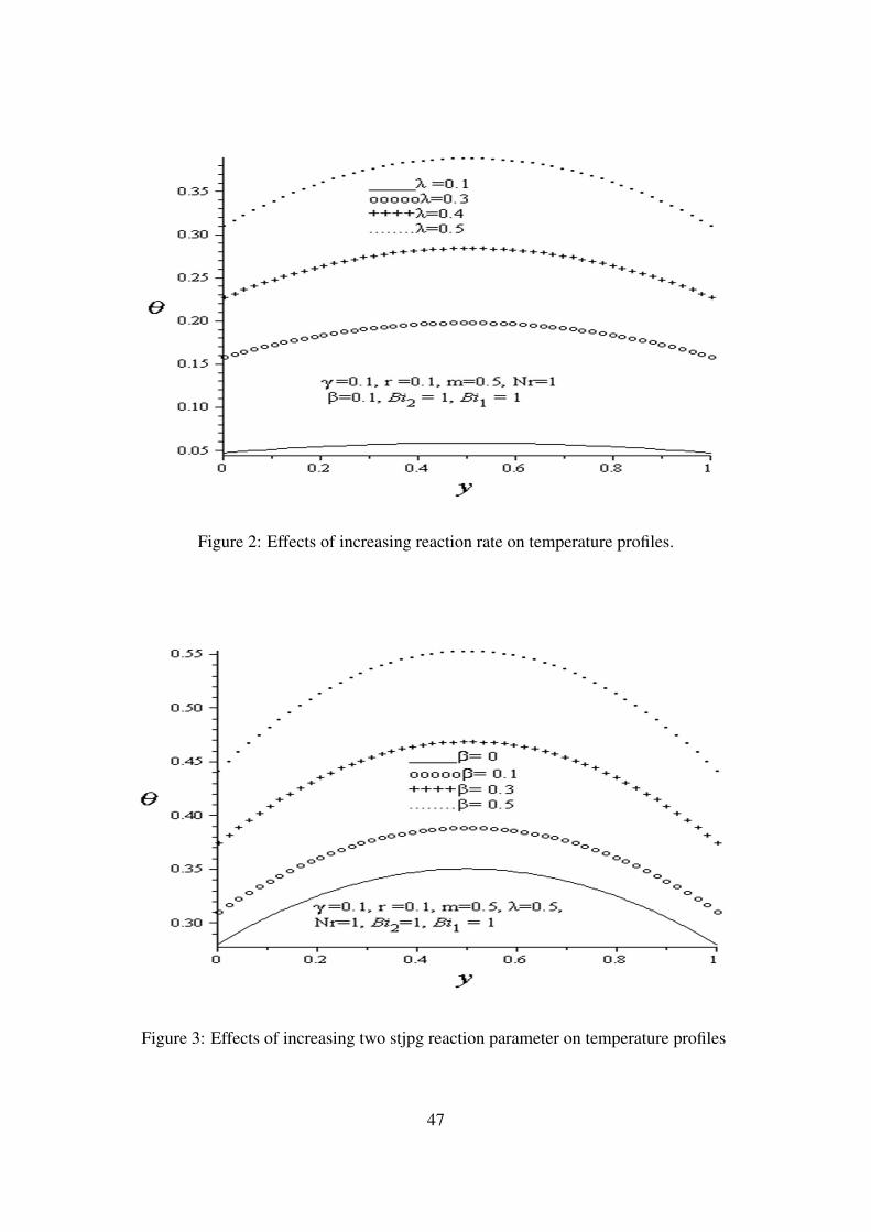
Figure 2: Effects of increasing reaction rate on temperature profiles.

Figure 3: Effects of increasing two stjpg reaction parameter on temperature profiles

47

Figure 4: Effects of increasing activation energy ratio parameter on temperature profiles

Figure 5: Effects of increasing radiative heat loss on temperature profiles

48

Figure 6: Effects of asymmetrical convective heat loss on temperature profiles

Figure 7: Effects of increasing radiative heat loss on critical value of λc

49

Figure 8: Effects of increasing convective heat loss on critical value of λc

Figure 9: Effects of two step reaction parameter on critical value of lambdac

50

4. ConclusionsHeat transfer analysis in a convecting and radiating two step reactive slab is presented. Themodel nonlinear governing differential equation is tackled numerically using Runge-Kutta-Fehlberg method with shooting iteration technique. Our results reveal among others, that thethermal runaway in the system is enhanced by two step exothermic reaction, while an increasein the convective and radiative heat loss stabilizes the system.

References[1] Bebernes J. and Eberly D, Mathematical problems from combustion theory. Springer-

Verlag, New York, (1989).

[2] Chambr P. L, On the solution of the PoissonBoltzmann equation with application to thetheory of thermal explosions. J. Chem. Phys. 20, 1795− 1797 (1952).

[3] Williams F. A, Combustion theory. Second Edition. Benjamin & Cuminy publishing Inc.Menlo Park, Califonia. (1985).

[4] Makinde O. D, Thermal stability of a reactive viscous flow through a porous-saturatedchannel with convective boundary conditions. Applied Thermal Engineering, 29, 1773−1777 (2009).

[5] Szabo Z. G, Advances in kinetics of homogeneous gas reactions. Methusen and Co. Ltd,Great Britain (1964).

[6] Frank-Kamenetskii D. A, Diffusion and heat transfer in chemical kinetics. Plenum Press,New York, (1969).

[7] Barenblatt G.I, Bell J. B, Crutchfield W. Y, The thermal explosion revisited. Proc. Natl.Acad. Sci. USA, 95, 13384− 13386, (1998).

[8] Sundn B, Transient in a composite slab by a time-varying incident heat-flux combinedwith convective and radiative cooling. Int. Commun. Heat Mass Transfer 13, 515 − 522,(1986).

[9] Makinde O. D, Exothermic explosions in a slab: A case study of series summation tech-nique. Int. Comm. Heat Mass Transfer, 31 (8), 1227− 1231(2004).

[10] Legodi A. M. K, Makinde O. D, A numerical study of steady state exothermic reaction ina slab with convective boundary conditions. Int. J. Phy. Sci. 6(10),2541− 2549, (2011).

[11] Makinde O. D, Hermite-Pade approach to thermal stability of reacting masses in a slabwith asymmetric convective cooling. Journal of the Franklin Institute, 349, 957 − 965,(2012).

[12] Makinde O. D, On the thermal decomposition of reactive materials of variable thermalconductivity and heat loss characteristics in a long pipe. Journal of Energetic Materi-als,30, 283− 298, (2012).

51

Non-Definite Sturm-Liouville Problems Two Turning Pointsby

Mervis Kikonko

University of Zambia,

Abstract

We study the non-definite Sturm-Liouville problem with a weight function having twoturning points on a finite closed interval. We find the piecewise smooth solution over theclosed interval and give the dispersion relation for the eigenvalues. The dispersion relationis then solved numerically using Maple software in order to calculate some eigenvalues.We also find the piecewise smooth eigenfunctions associated with each of the eigenvalues.Moreover, we present graphs of some of the eigenfunctions to check oscillation numbersof the eigenvalues associated with these functions. Finally, we point out a number ofinteresting open questions for further research

1. Introduction1.1 General Sturm-Liouville Theory

The Sturm-Liouville equation, named after Jacques Charles Francois Sturm (1803-1855) andJoseph Liouville (1809-1882) is a real second-order linear differential equation of the form

− (p (x)u′ (x))′+ q (x)u (x) = λw (x)u (x) , (1.1)

on the bounded or unbounded interval (α, β). The endpoints α and β can be finite or infinite,and u is a function of the independent variable x. The parameter λ (generally complex) forwhich the equation (1.1) has a solution u (non-identically zero) in (α, β) is called an eigenvalueand the corresponding function u is called an eigenfunction. In the case of a regular Sturm-Liouville problem, u is required to satisfy the boundary conditions

α1u (α) + α2p (α)u′ (α) = 0, (1.2)

β1u (β) + β2p (β)u′ (β) = 0, (1.3)

α1 and α2 are not both zero, similarly for β1 and β2. The functions p, q, w : [α, β] → <, havethe following properties:

p(x) > 0, q, w,1

p∈ L(α, β) and

β∫α

|w(s)|ds > 0.

Suppose that w(x) > 0, p(x), p′(x), q(x), and w(x) are continuous functions over the finiteinterval [α, β], then the eigenvalues λ1, λ2, λ3, . . . of problem (1.1),(1.2),(1.3) are real and canbe ordered such that λ1 < λ2 < λ3 < . . . < λn < . . . <∞. Also,corresponding to each eigen-value λn is a unique (up to a normalization constant) eigenfunction un(x), which has exactly nzeros in (α, β). The eigenfunction un(x) is called the nth fundamental solution satisfying theregular Sturm-Liouville problem (1.1)-(1.2)-(1.3).

52

Much has been written on Sturm-Liouville theory since the work of Sturm and Liouville in the19th century. In the period 1836−38, Sturm and Liouville published a remarkable set of paperswhich initiated the subject, which led to what is now called the qualitative theory of differentialequations, (see [3]). In the same book, the authors point out that, Sturm was mainly concernedwith the qualitative behavior of the eigenfunctions, while Liouville was more concerned withthe eigenfunction expansions.

This theory is important in applied mathematics, where SturmLiouville problems occur verycommonly. The differential equations considered here arise directly as mathematical models ofmotion according to Newton’s law, but more often as a result of using the method of separationof variables to solve the classical partial differential equations of physics, such as Laplace’sequation, the heat equation, and the wave equation. Sturm-Liouville problems have been dis-covered as describing the mathematics underlying a variety of physical phenomena. Thus theyhave been applied in various fields of study like Engineering and Physics.

1.2 General Non-Definite Sturm-Liouville Problems

Let (1.1) be written as

Tu = λwu, where T = − d

dx(p(x)

d

dx) + q(x). (1.4)

Then the problem (1.4)-(1.2)-(1.3) is called left-definite if the form (Tu,u) is definite on thedomain of definition for each u 6= 0. The problem is called right-definite if the form (wu,u)is definite. In the case that neither (Tu,u) nor (wu,u) is definite, then the problem is callednon-definite. Here, (,) denotes the inner product of the usual Hilbert space L2[α, β].

If we consider problem (1.1)-(1.2)-(1.3), and assume that w(x) changes sign on [α, β] and theproblem is non-definite, then the spectrum is discrete, always consists of a doubly infinite se-quence of real eigenvalues, has no finite limit point, and has at most a finite and even numberof non real eigenvalues (necessarily occurring in complex conjugate pairs) along with at mostfinitely many real non-simple eigenvalues (see e.g, [7]). Furthermore, the eigenfunction corre-sponding to the smallest positive eigenvalue need not necessarily be of one sign in (α, β). LetM be the number of pairs of distinct non-real eigenvalues of the problem and N be the numberof distinct negative eigenvalues of the same problem, then M ≤ N .

Moreover, there is an integer nR, called the Richardson index having the property that whenevern ≥ nR, there are exactly two eigenfunctions of the problem oscillating n-times in (α, β) (seee.g [7]). There is a positive number λ+, called the Richardson number defined asλ+ = infx ∈ < : ∀λ > x,

∫ βα|u(x, λ)|2w(x) dx > 0 (see [4]). Generally speaking, a non

definite problem will tend not to have a real ground state (positive eigenfunction) (see e.g [7]).If the positive eigenvalues λ+

n of a given non definite problem are labeled in such a way that λ+n

has an eigenfunction with precisely n zeros in (α, β), then

λ+n

n2∼ π2(∫ β

α

√(w(x)

p)+ dx

)2 , n→∞,

where (w(x)p

)+ = maxw(x)p, 0 is the positive part of w(x).

It is shown in [8] that if w(x) changes sign only once, then the roots of real and imaginary partsu, v of any non real eigenfuntion y = u + iv corresponding to a non real eigenvalue, separate

53

one another. Consequently, any non-real eigenfunction u of the problem cannot have a zero forx ∈ (α, β).

In this paper, we briefly present and discuss some of the results from my Master thesis [6](see Section 2). Furthermore, a final discussion and conclusion can be found in section 3. Inparticular, a number of interesting open questions are pointed out.

2. A Non definite Sturm-Liouville problem with weight function havingtwo turning pointsWe consider the Dirichlet problem

u′′ (x) + (λw (x) + q (x))u (x) = 0 (2.1)

on [-1,2] given by the boundary conditions

u (−1) = 0 = u (2) . (2.2)

Here, q (x) = q0 ∈ < for all x ∈ [−1, 2] and w(x) is a piecewise constant step-functiondescribed by the relations

w(x) =

a, if x ∈[-1,0],b, if x ∈(0,1],c, if x ∈(1,2],

where we assume, without loss of generality that, a < 0, b > 0, c < 0. We note that (2.1) is inSturm-Liouville form with q(x) replaced by −q(x).

Let H2[−1, 2] be the subspace of L2[−1, 2] consisting of all continuously differentiable func-tions u ∈ C ′[−1, 2] such that u′ is absolutely continuous on [-1,2] and u′′+ q(x)u ∈ L2[−1, 2].Let T be the linear operator in L2[−1, 2] defined by

D(T ) =u ∈ H2[−1, 2] |u(−1) = 0 = u(2)

Tu = u′′ + q(x)u. (2.3)

We have the following result:

Theorem 2.4 The forms (Tu, u) and (wu, u) arising from the operator T defined by (2.3) aregenerally indefinite.

54

Proof: We have

(Tu, u) =

2∫−1

(u′′ + q(x)u)udx

=

2∫−1

u′′udx+

2∫−1

q(x)|u|2dx

= −2∫

−1

u′u′dx+

2∫−1

q(x)|u|2dx

=

2∫−1

(q(x)|u|2 − |u′|2)dx.

From the above result, we deduce that for q ≤ 0, (Tu, u) < 0 for all u ∈ D(T ) which meansthat −T ≥ 0. However, when q > 0, we see that the form (Tu, u) may be sign-indefinite.By Sturm-Liouville theory we recall that there are always infinitely many eigenvalues havinga fixed sign (positive or negative). Let us choose q so that T has both positive and negativeeigenvalues. Then, it is easy to see that if we choose u to be an eigenfunction correspondingto a positive eigenvalue of T (defined by (2.3)) then (Tu, u) > 0. On the other hand, byassumption, since T has a negative eigenvalue with eigenfunction v then (Tv, v) < 0. So, fixingsuch a general value of q, there may exist functions u for which (Tu, u) > 0 and a possiblydifferent set of u’s for which (Tu, u) < 0 and so the form (Tu, u) is generally indefinite.

Similarly,

(wu, u) =

2∫−1

w|u|2dx

= −|a|0∫

−1

|u|2dx+ b

1∫0

|u|2dx− |c|2∫

1

|u|2dx.

It is clear that the sign of λ(wu, u) is indefinite since it generally depends on the relative sizesof a, b, c. Thus, both forms are indefinite.

The proof is complete.

Therefore, in accordance with accepted terminology (see [8]), the problem (2.1),(2.2) is non-definite.

2.1 Explicit solution for the problem(2.1),(2.2) and results

For the special case with a = −1, b = 2, c = −1, we found the explicit solution of (2.1),(2.2)given below

u(x) =

X(x), if x ∈[-1,0],Y (x), if x ∈(0,1],Z(x), if x ∈(1,2],

55

Table 1: Summary of results of the spectrum of problem (2.1)-(2.2)q0 ] of complex pairs ] of negative eigenvalues total ] of eigenvalues Smallest oscillation ]π2 1 9 18 22π2 3 6 18 33π2 3 7 18 35π2 4 6 20 46π2 4 7 20 5

where a < 0, b > 0, c < 0, and

X(x) =sin(√−λ|a|+ q0(x+ 1))√−λ|a|+ q0

Y (x) =

√λb+ q0 sin(

√−λ|a|+ q0) cos(

√λb+ q0x)√

−λ|a|+ q0

√λb+ q0

+

√−λ|a|+ q0 cos(

√−λ|a|+ q0) sin(

√λb+ q0x)√

−λ|a|+ q0

√λb+ q0

Z(x) =sin(√−λ|a|+ q0) cos(

√λb+ q0) cos(

√−λ|c|+ q0(x− 1))√

−λ|a|+ q0

+cos(

√−λ|a|+ q0) sin(

√λb+ q0) cos(

√−λ|c|+ q0(x− 1))√

λb+ q0

+cos(

√−λ|a|+ q0) cos(

√λb+ q0) sin(

√−λ|c|+ q0(x− 1))√

−λ|c|+ q0

−√λ|b| − q0 sin(

√−λ|a|+ q0) sin(

√λb+ q0) sin(

√−λ|c|+ q0(x− 1))√

−λ|a|+ q0

√−λ|c|+ q0

.

The solution is found by piecing together the various solutions on the intervals (-1,0), (0,1) and(1,2) so as to obtain a continuously differentiable function on (-1,2). By solving the dispersionrelation

0 =√−λ|c|+ q0

√λb+ q0 sin(

√−λ|a|+ q0) cos(

√λb+ q0) cos(

√−λ|c|+ q0)

+√−λ|c|+ q0

√−λ|a|+ q0 cos(

√−λ|a|+ q0) sin(

√λb+ q0) cos(

√−λ|c|+ q0)

+√−λ|a|+ q0

√λb+ q0 cos(

√−λ|a|+ q0) cos(

√λb+ q0) sin(

√−λ|c|+ q0)

−(λb+ q0) sin(√−λ|a|+ q0) sin(

√λb+ q0) sin(

√−λ|c|+ q0).

we calculated a few eigenvalues in the cases q0 = π2, 2π2, 3π2, 5π2 and 6π2 in the rectangleD = λ ∈ C : |<λ| < 300 and |=λ| < 300 using the Maple package RootFinding[Analytic].Tables 1 and 2 show summaries of the results on the spectrum.

56

Table 2: Non-real eigenvalues obtained inside the rectangle D for the cases q0 =π2, 2π2, 3π2, 5π2, 6π2

No. of zeros ofq0 Eigenvalues Re u(x, λi) Im u(x, λi)

π2 3.2465± 5.6334i 3 1

2π2

−8.307± 5.5991i 4 2−4.220± 5.7435i 3 312.940± 6.6651i 4 2

3π2 5.1614± 7.7537i 4 4−2.452± 10.506i 5 3

5π2

7.0223± 10.935i 6 420.750± 12.134i 5 5−19.75± 7.2174i 6 4−16.37± 10.338i 5 5

6π2

−6.434± 14.431i 6 6−13.40± 13.525i 7 552.026± 7.0997i 6 421.552± 15.247i 7 5

5π2

7.0223± 10.935i 6 420.750± 12.134i 5 5−19.75± 7.2174i 6 4−16.37± 10.338i 5 5

6π2

−6.434± 14.431i 6 6−13.40± 13.525i 7 552.026± 7.0997i 6 421.552± 15.247i 7 5

2.2 Example( the case q0 = 6π2)

The asymptotic distribution of the eigenvalues satisfies

λ+n

n2∼ π2(∫ 2

−1

√w+(x) dx

)2 ≈ 4.9348, n→∞.

In this case, the Richardson index is 5 and from the data we see that λ+ ≤ 106.4765 while theoscillation number for λ = 106.4765 is 5, and so the Richardson index is 5, as expected.

3. Discussion and conclusion3.1 Discussion

In all the cases considered in this paper, we have both real and non-real eigenvalues. It canbe seen from the graphs of the eigenfunctions that generally oscillation numbers decrease asthe parameter value increases, but then oscillations will stabilize and then the usual oscillationtheorem may be claimed. This leads to the estimation of λ+ and nR.

For example in figure 1, we see that the oscillation number of the smallest positive eigenvalueis greater than that of the second one. However, oscillations stabilize from the third onwards,

57

(a) λ = 22.801778 (b) λ = 49.348022 (c) λ = 106.476595

(d) λ = 166.681017 (e) λ = 235.752859

Figure 1: eigenfunctions corresponding to positive eigenvalues for the case q0 = 6π2

(a) Real Part (b) Imaginary Part (c) Real Part (d) Imaginary Part

Figure 2: The cases λ = −6.4344− 14.4314i, λ = −13.4034− 13.5248i

(a) Real Part (b) Imaginary Part (c) Real Part (d) Imaginary Part

Figure 3: The casesλ = 21.5520− 15.2468i, λ = 52.0258 + 7.0997i

that is, for all positive eigenvalues such that λ ≥ 106.476595 each eigenvalue has a uniqueoscillation number. This shows that λ+ ≤ 106.476595 and nR = 5.

Generally speaking, the number of non-real eigenvalues seems to increase with increasing q0.The number of pairs of distinct non-real eigenvalues of the problem does not exceed the numberof negative eigenvalues in all the cases considered. For all values of q0 considered (cases

58

where there are non-real eigenvalues), the smallest oscillation number is 2 and so there is nopositive eigenfunction in (-1,2). Furthermore, the real and imaginary parts of the non-realeigenfunctions do not have interlacing zeros. It is evident from the graphs in figures 2 and 3that the number of zeros of the imaginary part is less than that of the real part by 2 in somecases, and equal in other cases. However, the non-real eigenfunctions do not vanish in (-1,2).

3.2 Conclusion

A huge number of papers by mathematicians and others, have been published on Sturm-Liouvilleproblems since their origins in 1836. Yet, remarkably, this subject is still an intensely activefield of research today. In this paper, we undertook a numerical study of the non-real eigen-functions and eigenvalues of a non-definite Sturm-Liouville problem with two turning points,paralleling the study in [4] in the case of one turning point. Ultimately, our aim was to examinethe behavior of the eigenfunctions, both real and non-real, of this non-definite Sturm-Liouvilleproblem.

One feature of the non-definite problem is the possible existence of non-real eigenvalues. Thismay sound paradoxical, as the equation is (formally) self-adjoint and so all eigenvalues shouldbe real. However, this is where the problem lies: the formal self-adjointness of an equationdoes not necessarily imply the self-adjointness of the corresponding operator. It follows thatwhenever there is a non-real eigenvalue the corresponding operator cannot be self-adjoint in aHilbert space.

We have indeed verified that if the problem (3.1)-(3.2) has at least one (complex conjugate)pair of non-real eigenvalues, then there is no real eigenvalue whose corresponding eigenfunc-tion has one zero in the interval (−1, 2) (in conformity with the results in [2], [1]). We alsoshowed that, in the cases considered here, the complex eigenfunctions (corresponding to non-real eigenvalues) are never zero in (−1, 2). Whether this is an accident or the result of a moregeneral yet unproven theorem, is unknown, but we strongly believe it is so and pose this as anopen question for future research.

For these same examples, we also showed that the real and imaginary parts of these eigenfunc-tions do not have interlacing zeros (although they are expected to since the non real eigenfunc-tions do not vanish). In fact, these zeros interlace in the one-turning-point case as shown byRichardson (see [8]). However, in the case of two turning points we see that there are exampleswhere the zeros do not interlace at all. This fact too, raises an interesting open question forfuture research.

Furthermore, the number of zeros of the real part of each of the non-real eigenfunctions con-sidered is greater than or equal to the number of zeros of the imaginary part. This may alsobe a consequence of a more general theorem which we don’t know, so then, we have a thirdinteresting open question. In future studies on this subject, there is need for the formulationof general theorems that could explain some or all of these observations. Finally, we observedthat even for real eigenvalues the corresponding eigenfunctions do not behave in conformitywith the Sturm oscillation theorem as was postulated and proved by Haupt (1911) in [5], andRichardson [8].

ACKNOWLEDGEMENTS: I should like to express my special thanks to my Master of Science thesissupervisor Dr. Angelo B. Mingarelli (Carleton University, Ottawa, Canada) for suggesting the topic.Working under his supervision was a pleasure and a good experience. I feel greatly honored to still have

59

him supervise my PhD research in which he is co-supervising with Professor Lars-Erik Persson andProfessor Peter Wall both from Lulea University of Technology. I thank the three professors for readingthrough my manuscript and giving valuable suggestions and comments.

References[1] W. Allegretto and A. B. Mingarelli. On the non-existence of positive solution for a Schrodinger

equation with an indefinite weight-function. C. R. Math. Rep. Acad. Sci. Canada, 8:69–72, 1986.

[2] W. Allegretto and A. B. Mingarelli. Boundary problems of the second order with an indefiniteweight-function. J. Reine Angew. Math., 398:1–24, 1989.

[3] T. G. Anderson, R. C. Brown, and D. B. Hinton. Perturbation theory for a one-term weighteddifferential operator. In Spectral theory and computational methods of Sturm-Liouville problems(Knoxville, TN, 1996), volume 191 of Lecture Notes in Pure and Appl. Math., pages 149–170.Dekker, New York, 1997.

[4] F.V Atkinson and D Jabon. Indefinite Sturm-Liouville problems. In Proceeding of the 1984 work-shop on Spectral Theory of Sturm-Liouville Differential Operators, pages 31–44. Argon NationalLaboratory, Argon,Illinois, 1984.

[5] O. Haupt. Untersuchungen uber Oszillationstheoreme. Diss. Wurzburg. Leipzig: B. Z. Teubner. 50S. 8 , 1911.

[6] M. Kikonko. Non Definite Sturm-Liouville problem with weight function having two turning points.Thesis (Masters). Carleton University, 2011.

[7] A.B. Mingarelli. A survey of the regular weighted Sturm-Liouville problem—the nondefinite case.In International workshop on applied differential equations (Beijing, 1985), pages 109–137. WorldScientific Publishing, Singapore, 1986.

[8] R. G. D. Richardson. Contributions to the Study of Oscillation Properties of the Solutions of LinearDifferential Equations of the Second Order. Amer. J. Math., 40(3):283–316, 1918.

60

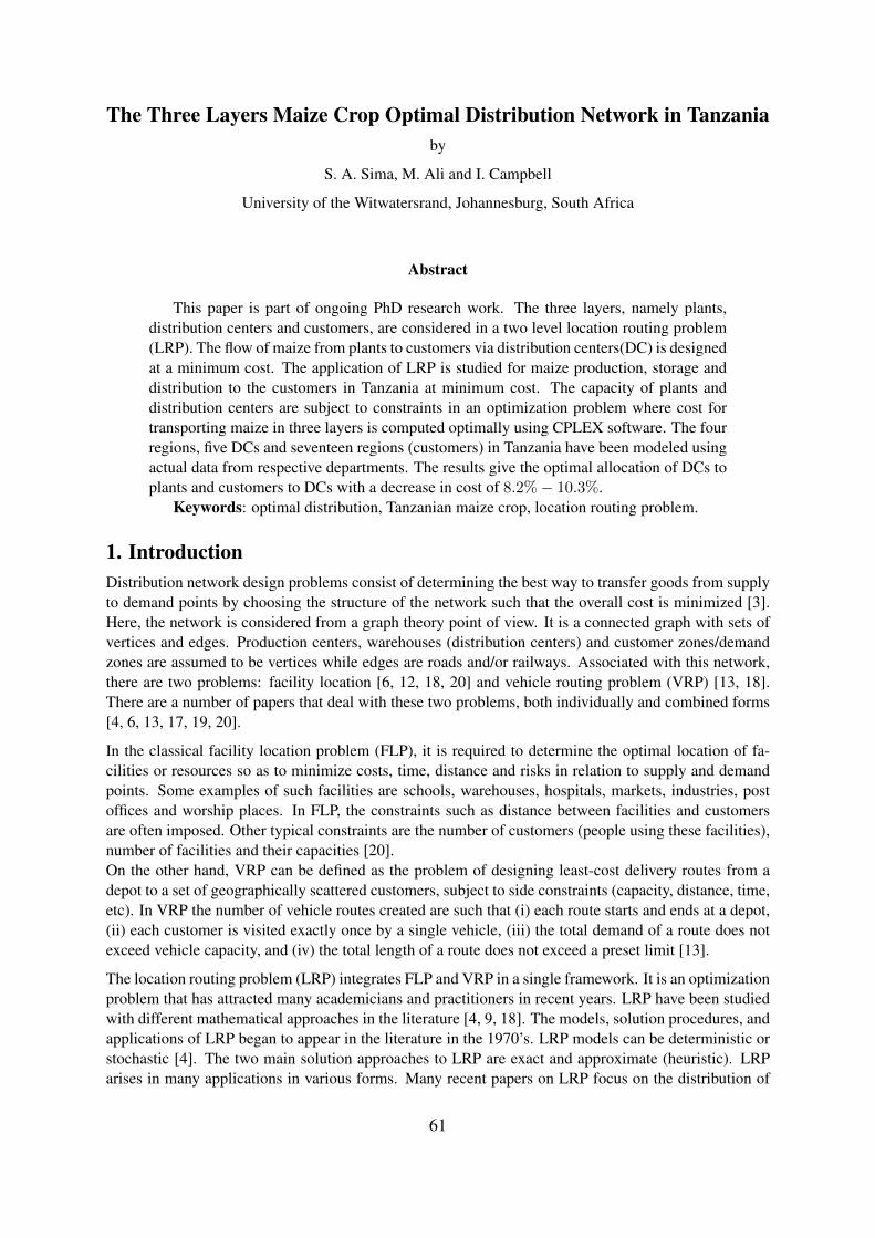
The Three Layers Maize Crop Optimal Distribution Network in Tanzaniaby

S. A. Sima, M. Ali and I. Campbell

University of the Witwatersrand, Johannesburg, South Africa

Abstract

This paper is part of ongoing PhD research work. The three layers, namely plants,distribution centers and customers, are considered in a two level location routing problem(LRP). The flow of maize from plants to customers via distribution centers(DC) is designedat a minimum cost. The application of LRP is studied for maize production, storage anddistribution to the customers in Tanzania at minimum cost. The capacity of plants anddistribution centers are subject to constraints in an optimization problem where cost fortransporting maize in three layers is computed optimally using CPLEX software. The fourregions, five DCs and seventeen regions (customers) in Tanzania have been modeled usingactual data from respective departments. The results give the optimal allocation of DCs toplants and customers to DCs with a decrease in cost of 8.2%− 10.3%.

Keywords: optimal distribution, Tanzanian maize crop, location routing problem.

1. IntroductionDistribution network design problems consist of determining the best way to transfer goods from supplyto demand points by choosing the structure of the network such that the overall cost is minimized [3].Here, the network is considered from a graph theory point of view. It is a connected graph with sets ofvertices and edges. Production centers, warehouses (distribution centers) and customer zones/demandzones are assumed to be vertices while edges are roads and/or railways. Associated with this network,there are two problems: facility location [6, 12, 18, 20] and vehicle routing problem (VRP) [13, 18].There are a number of papers that deal with these two problems, both individually and combined forms[4, 6, 13, 17, 19, 20].

In the classical facility location problem (FLP), it is required to determine the optimal location of fa-cilities or resources so as to minimize costs, time, distance and risks in relation to supply and demandpoints. Some examples of such facilities are schools, warehouses, hospitals, markets, industries, postoffices and worship places. In FLP, the constraints such as distance between facilities and customersare often imposed. Other typical constraints are the number of customers (people using these facilities),number of facilities and their capacities [20].On the other hand, VRP can be defined as the problem of designing least-cost delivery routes from adepot to a set of geographically scattered customers, subject to side constraints (capacity, distance, time,etc). In VRP the number of vehicle routes created are such that (i) each route starts and ends at a depot,(ii) each customer is visited exactly once by a single vehicle, (iii) the total demand of a route does notexceed vehicle capacity, and (iv) the total length of a route does not exceed a preset limit [13].

The location routing problem (LRP) integrates FLP and VRP in a single framework. It is an optimizationproblem that has attracted many academicians and practitioners in recent years. LRP have been studiedwith different mathematical approaches in the literature [4, 9, 18]. The models, solution procedures, andapplications of LRP began to appear in the literature in the 1970’s. LRP models can be deterministic orstochastic [4]. The two main solution approaches to LRP are exact and approximate (heuristic). LRParises in many applications in various forms. Many recent papers on LRP focus on the distribution of

61

consumer goods [2, 6, 10, 12, 15–18, 22]. This network is a two level LRP as the routes occur betweenthe first layer (plants) and the second layer (distribution centers), and also between the second layer andthe third layer (customers). If there is more than one level of routing involved in LRP, then it is calledmulti-level LRP. The problem we study here is a two-level LRP.

The practical problem at hand is a deterministic model which is part of a PhD work in progress.

The problem is formulated mathematically as a mixed integer linear programming problem which wasthen solved using actual data. The considered practical example has a number of unique features whichmake the research worthwhile . In particular, maize crop (single commodity) transportation in Tanzaniais considered as an application of the two-level LRP. So our study is three folds: First, we model theoptimization problem as a two-level LRP; Second, we design an algorithm to solve such model and thirdwe consider its practical application. This is the first application of LRP to a practical and real problemin Tanzania.

In the next section we present the deterministic mathematical model for a multi-level LRP. Section 3presents the maize production and distribution network in Tanzania, and the research data and solutionapproach is in Section 4. The last section, 5, presents conclusion and recommendations.

In this research, we use plant and production center, warehouse and distribution center, and customer anddemand zones, interchangeably. The distribution centers or warehouses are also referred to as depots.

2. The deterministic mathematical model for multi-level LRPThe multi-level LRP models explored in the literature, are either single-commodity or multi-commodity.We now present the mathematical model for a multi-level LRP dealing with a single commodity. Themodel is adapted from Elhedhli et al [7] and the references [8, 12, 14]. The multi-commodity modelused by Elhedhli.

Data for the model:j: index for plants, where j = 1, 2, ..., J . J is the total number of plants.k: index for possible distribution center sites, where k = 1, 2, ...,K. K is the total number of the candi-date distribution center sites.l: index for customer demand zones, where l = 1, 2, ..., L. L is the total number of customer demandzones.Sj : supply (production capacity) for a product at plant j.Dl: demand of product at customer zone l.Vk: maximum capacity for DC at site kCjk: average unit cost of shipping (routing) a product from plant j to DC k.Ckl: average unit cost of shipping a product from DC k to customer zone l.fk: fixed cost of the annual possession and operating cost for a DC at site k.

Decision variables for the model:Xjk: amount of product shipped from plant j to DC k.Ykl: 1 if the DC k serves customer zone l, and 0 otherwise.Zk: 1 if a DC k is opened at site k, and 0 otherwise.

The formulated mixed integer linear programming model is as follows:

min∑jk

CjkXjk +∑kl

CklDlYkl +∑k

fkZk (2.1)

62

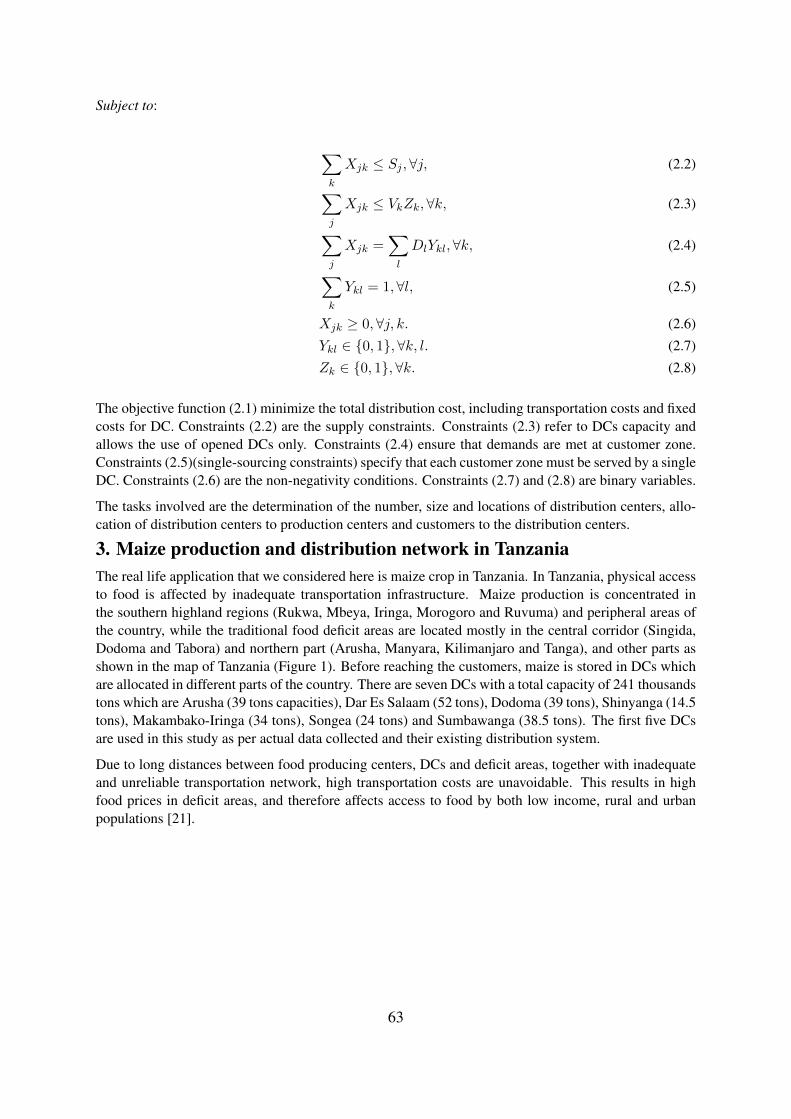
Subject to:

∑k

Xjk ≤ Sj , ∀j, (2.2)∑j

Xjk ≤ VkZk,∀k, (2.3)

∑j

Xjk =∑l

DlYkl,∀k, (2.4)

∑k

Ykl = 1,∀l, (2.5)

Xjk ≥ 0,∀j, k. (2.6)

Ykl ∈ 0, 1, ∀k, l. (2.7)

Zk ∈ 0, 1,∀k. (2.8)

The objective function (2.1) minimize the total distribution cost, including transportation costs and fixedcosts for DC. Constraints (2.2) are the supply constraints. Constraints (2.3) refer to DCs capacity andallows the use of opened DCs only. Constraints (2.4) ensure that demands are met at customer zone.Constraints (2.5)(single-sourcing constraints) specify that each customer zone must be served by a singleDC. Constraints (2.6) are the non-negativity conditions. Constraints (2.7) and (2.8) are binary variables.

The tasks involved are the determination of the number, size and locations of distribution centers, allo-cation of distribution centers to production centers and customers to the distribution centers.

3. Maize production and distribution network in TanzaniaThe real life application that we considered here is maize crop in Tanzania. In Tanzania, physical accessto food is affected by inadequate transportation infrastructure. Maize production is concentrated inthe southern highland regions (Rukwa, Mbeya, Iringa, Morogoro and Ruvuma) and peripheral areas ofthe country, while the traditional food deficit areas are located mostly in the central corridor (Singida,Dodoma and Tabora) and northern part (Arusha, Manyara, Kilimanjaro and Tanga), and other parts asshown in the map of Tanzania (Figure 1). Before reaching the customers, maize is stored in DCs whichare allocated in different parts of the country. There are seven DCs with a total capacity of 241 thousandstons which are Arusha (39 tons capacities), Dar Es Salaam (52 tons), Dodoma (39 tons), Shinyanga (14.5tons), Makambako-Iringa (34 tons), Songea (24 tons) and Sumbawanga (38.5 tons). The first five DCsare used in this study as per actual data collected and their existing distribution system.

Due to long distances between food producing centers, DCs and deficit areas, together with inadequateand unreliable transportation network, high transportation costs are unavoidable. This results in highfood prices in deficit areas, and therefore affects access to food by both low income, rural and urbanpopulations [21].

63

Figure 1: The map of Tanzania showing the food production centers, warehouses and deficitareas

This study is useful as it provides a mechanism for reducing food prices within the country. This willcontribute to the June 2009 Tanzania policy involving priority of agriculture also known as ‘AgricultureFirst’ (Kilimo Kwanza) and as stipulated in ten implementation pillars. For instance, one of the pillarsinvolves identification of priority areas for strategic food commodities to increase the country’s foodself sufficiency. The pillars mention a price stabilization mechanism, which includes the expansion ofstorage capacity and improvement of railway and road systems [1]. In the 2012/2013 Ministry of Agri-culture budget speech, the price stabilization for maize flour in cities was addressed, after the price had

64

decreased by 38% to 40%. This was as a result of about 41,000 tons of maize from warehouses beingsold to public markets in regional cities/municipal to cater for a maize deficit [5].

4. Research data and solution approachThe two-level LRP model is a commodity customer delivery model with the following assumptions:(i) demands in each customer zone is known, (ii) number of plants, capacities and their locations areknown, (iii) all possible warehouses, their capacities and locations are to be redetermined optimally, (iv)transportation costs from plants to warehouses and from warehouses to customers are known.

Optimization is carried out to determine the values of the decision variables in the model. The optimaldecisions to be made are: (i) number of distribution centers, capacities and their locations, (ii) allocationof distribution centers to plants, (iii) allocation of customers to distribution centers, (iv) routes designingfrom plants to distribution centers and from distribution centers to customers with their associated costs.

4.1 Research data

The food security system in Tanzania is based on maize production, storage and final distribution to thecustomers. The required data for the model is from several sources; .All sources of data are based in Tanzania

• Tanzania National Roads Agency (TANROADS: Road distances between regions as per March2009 and road classification (collected in January, 2011).

• Ministry of Agriculture, Food Security and Cooperatives: Maize production capacity and surplusfrom ”Volume 1: The 2010/11 Final Food Crop Production Forecast for 2011/12 Food SecurityEXECUTIVE SUMMARY”. This is accessible fromhttp://www.kilimo.go.tz/publications.

• National Food Reserve Agency (NFRA): Warehouses capacity and transfer quantities from plantsto warehouses in 2009/2010 (Obtained in January, 2011).

• Prime Minister Office-Disaster Department: Regional demand quantities of maize between 2004and 2010 and distances between DCs and demand zones (districts). The maximum annual demandin each region had been considered in this work. The data is as presented in Table 1 and 2.

Table 1: Plants and DCs: Distances (’000km) and Capacities (’000Mt)Plants DCs - Road Distances Capacity No of DCs

Arusha D’Salaam Dodoma Makambako ShinyangaIringa 0.689 0.492 0.264 0.12 0.802 100 3Mbeya 1.02 0.822 0.594 0.21 0.761 251 7Rukwa 1.348 1.15 0.922 0.538 0.79 140 4Ruvuma 1.144 0.947 0.719 0.335 1.257 41 1DC ca-pacity.

39 52 39 34 14.5

Total production capacity 532Total DCs Capacity 178.5

65

Table 2: DCs and Customers: Distances (’000’km) and demands (’000’Mt)S/N Cust/DC Arusha Dar Dodoma Makambako Shinyanga Customer

Demand1 Arusha 0.071 0.717 0.496 0.88 0.695 14.3782 Coast 0.734 0.088 0.539 0.7 1.077 8.6263 Dodoma 0.495 0.521 0.07 0.454 0.608 15.2164 Iringa 0.728 0.621 0.403 0.139 0.941 7.0085 Kagera 1.137 1.502 1.051 1.433 0.513 1.5596 Kilimanjaro 0.125 0.611 0.55 0.934 0.749 8.9407 Lindi 1.185 0.539 0.99 1.151 1.528 4.0938 Manyara 0.229 0.875 0.318 0.809 0.517 15.2149 Mara 1.133 1.498 1.047 1.431 1.509 11.497

10 Mbeya 0.997 0.8 0.572 0.188 1.11 2.83511 Morogoro 0.814 0.385 0.452 0.613 0.89 7.68912 Mtwara 1.256 0.61 1.061 1.17 1.599 3.87613 Mwanza 0.863 1.228 0.777 1.161 0.289 10.39814 Shinyanga 0.725 1.19 0.639 1.024 0.101 9.70215 Singida 0.662 0.688 0.237 0.621 0.493 9.43416 Tabora 0.807 1.209 0.721 1.105 0.183 5.77317 Tanga 0.772 0.337 0.788 0.756 1.066 8.906

DC CustomerCapacity

5 6 5 4 2

Average demand 8.538Total Demand 145.144

66

In table 1 the values in the last column (No of DCs) were obtained by dividing the relevant plant capacityby average DC capacity. The demands in the last column of table 2, were obtained from 93 districts’demands in Tanzania. The given districts demand were then summed in each region to have a regionalcustomer demand. The last row of this table gives the number of customers (from 17 customers) thatcan be saved by the particular DC (DC customer capacity). The serial number, 1-17 in table 2 is codedas corresponding customer (customers saved) in the programming results from table 3, 4 and 5.

4.2 Solution approach and computational results

The solution of a mixed integer linear programming deterministic model is obtained by using CPLEXsoftware. The real life data from Tanzania in tables 1 and 2 was used. The problem was solved intwo stages. The first stage is solved as a FLP or DC location problem, where DCs and customers areinvolved. The second stage considered all three layers simultaneously as a two level LRP. The solutionobtained is optimal, hence it is an exact method.

Facility Location Problem solutionIn the FLP, the target is to find the optimal number and location of warehouses with respect to distancefrom customers and their capacities while satisfying customers’ demands at minimum cost. The modelfor this case is:

min∑kl

CklDlYkl +∑k

fkZk (4.1)

Subject to constraint sets (2.4), (2.5),(2.7) and (2.8). Using CPLEX software (IBM ILOG CPLEXOptimization Studio), several results were obtained by changing the capacity of warehouses from theexisting capacities and observing the influence on the fixed cost. Some important results are summarisedbelow.

Table 3: Results for changing capacities of DC while fixed cost is ZERODC/RUN R1 (6,5,5,4,2: Existing

Cap). Customers savedR2 (4,5,3,1,5: Actualmax use). Customerssaved

R3 (6,5,5,2,4 =6,5,4,2,5). Customerssaved

Dar 2, 7, 11, 12, 17 2, 7, 12, 17 2, 7, 11, 12, 17Arusha 1, 6, 8 1, 6, 8, 9 1, 6, 8Dodoma 3, 5, 9, 13, 15 3, 4, 11 3, 9, 15Makambako 4, 10 10 4, 10Shinyanga 14, 16 5, 13, 14,15, 16 5, 13, 14, 16ObjectiveValue (km)

6.177 5.824 5.151

Run Time(Sec)

8 16 10

NOTE: All warehouses are open and all customers are saved

From table 3 where fixed cost is zero, R1, R2 and R3 are three runs (computations) with different resultsfrom different capacities of DCs. R1 consider the existing capacities as constructed, R2 is maximumuse of the DC as per 2004-2010 demands. R3 is optimal location and capacities as from objective value(last but one row). First it shows all DCs are open, and all customers (total 17) are allocated to DCs.The optimal capacities require the Makambako DC to save 2 customers and Shinyanga DC to save 4 or5 customers with objective value of 5.151km. This result of having 1.026km (1,026km) (savings) for

67

Table 4: Results for changing capacities of DC while fixed (f) cost is 10 for each DC.DC/RUN R1 (6,5,5,4,2:

Existing Cap).Customerssaved

R2 (4,5,3,1,5:Actual max use).Customers saved

R3 (6,5,5,2,4).Customers saved

R4 (6,5,6,1,4).Customers saved

Dar 2, 7, 11, 12, 17 2, 7, 12, 17 2, 7, 11, 12, 17 2, 4, 7, 11, 12, 17Arusha 1, 6, 8, 9, 16 1, 4, 6, 8, 9 1, 6, 8 1, 6, 8, 9, 16Dodoma 3, 4, 10, 13, 15 3, 10, 11 3, 4, 9, 10, 15 3, 5, 10, 13, 14,

15Makambako - - - -Shinyanga 5, 14 5, 13, 14,15, 16 5, 13, 14, 16 -Objective Value(km)

46.997 46.533 45.799 38.291

Run Time (Sec) 17 9 17 8NOTE: At least one warehouse is closed for f ≥ 0.3 and all customers are saved

constructed capacity and 673km for maximum use DC capacity. The customers as per each DC can bedesigned a direct route from allocated DC.

Table 4 results indicates the influence of fixed costs in FLP where only 3 DC are to be opened in theoptimal costs. As shown in last column, the objective value is 38.291km, that is less by 8.706km and8.242km from constructed capacities and maximum use capacities respectively.

The two level LRP solutionThis is a second stage solving where plants, warehouses and customers distribution cost are now con-sidered simultaneously. Minimum cost attained by optimal location of warehouses to plants and alsocustomers to open warehouses. In this case, all the five warehouses are open for both capacities andfixed cost consideration contract to first stage.

The whole model (2.1) to (2.8) is used with some modification of decision variable from quantities toa binary. Xjk is now 1 if a transfer from plants to open warehouse, and 0 otherwise. So we have anadditional single source constraints to link plants and warehouses as:∑

j

Xjk = 1, ∀k. (4.2)

The most important computational results are summarised in the table 5.

From all runs conducted, the optimal DCs allocation to plants are; Iringa plant supplies to Dar, Arushaand Dodoma, and Makambako and Shinyanga supplied by Mbeya plant. This is from the fact that theplants capacities are more than sufficient as compared to DCs’ capacities (See table 1). The Ruvumaand Rukwa plants remain untouched!

Table 5 results as indicated, optimal location and allocation attained with objective value of 7.567km forzero fixed costs and 57.567km for f = 10 where capacities of Makambako and Shinyanga in particularare redetermined. The optimal computed objective value is 11.9% and 8.2% less than constructed andmaximum use capacities respectively. For both zero and non zero fixed costs, all DCs are to be opened.So the two level LRP is solved with 8.2% - 11.2% saving costs. The direct routes are then designed fromoptimal location and allocation as resulted from computations.

68

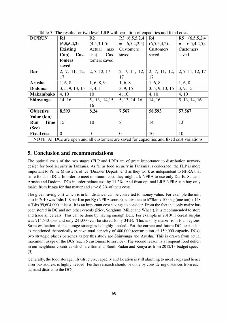
Table 5: The results for two level LRP with variation of capacities and fixed costsDC/RUN R1

(6,5,5,4,2:ExistingCap). Cus-tomerssaved

R2(4,5,3,1,5:Actual maxuse). Cus-tomers saved

R3 (6,5,5,2,4= 6,5,4,2,5)Customerssaved

R4(6,5,5,4,2).Customerssaved

R5 (6,5,5,2,4= 6,5,4,2,5).Customerssaved

Dar 2, 7, 11, 12,17

2, 7, 12, 17 2, 7, 11, 12,17

2, 7, 11, 12,17

2, 7, 11, 12, 17

Arusha 1, 6, 8 1, 6, 8, 9 1, 6, 8 1, 6, 8 1, 6, 8Dodoma 3, 5, 9, 13, 15 3, 4, 11 3, 9, 15 3, 5, 9, 13, 15 3, 9, 15Makambako 4, 10 10 4, 10 4, 10 4, 10Shinyanga 14, 16 5, 13, 14,15,

165, 13, 14, 16 14, 16 5, 13, 14, 16

ObjectiveValue (km)

8.593 8.24 7.567 58.593 57.567

Run Time(Sec)

15 10 8 14 13

Fixed cost 0 0 0 10 10NOTE: All DCs are open and all customers are saved for capacities and fixed cost variations

5. Conclusion and recommendationsThe optimal costs of the two stages (FLP and LRP) are of great importance to distribution networkdesign for food security in Tanzania. As far as food security in Tanzania is concerned, the FLP is moreimportant to Prime Minister’s office (Disaster Department) as they work as independent to NFRA thatstore foods in DCs. In order to meet minimum cost, they might ask NFRA to use only Dar Es Salaam,Arusha and Dodoma DCs in order reduce cost by 11.2%. And from optimal LRP, NFRA can buy onlymaize from Iringa for that matter and save 8.2% of their costs.

The given saving cost which is in km distance, can be converted to money value. For example the unitcost in 2010 was Tshs 148 per Km per Kg (NFRA source), equivalent to 673km x 1000kg (one ton) x 148= Tshs 99,604,000 at least. It is an important cost savings to consider. From the fact that only maize hasbeen stored in DC and not other cereals (Rice, Sorghum, Millet and Wheat), it is recommended to storeand trade all cereals. This can be done by having enough DCs. For example in 2010/11 cereal surpluswas 714,543 tons and only 241,000 can be stored (only 34%). This is only maize from four regions.So re-evaluation of the storage strategies is highly needed. For the current and future DCs expansionas mentioned theoretically to have total capacity of 400,000 (construction of 159,000 capacity DCs),two strategic places or zones as per this study are Shinyanga and Arusha. This is drawn from actualmaximum usage of the DCs (each 5 customers to service). The second reason is a frequent food deficitin our neighbour countries which are Somalia, South Sudan and Kenya as from 2012/13 budget speech[5].

Generally, the food storage infrastructure, capacity and location is still alarming to most crops and hencea serious address is highly needed. Further research should be done by considering distances from eachdemand district to the DCs.

69

References[1] Agriculture first document. http://www.tzonline.org/pdf/tenpillarsofkilimokwanza.pdf (accessed

on 07/05/2010), 2009.

[2] Ahuja, R., Magnanti, T. L. and Orlin, J. B. Network flows: Theory, algorithms and applications.Prentice Hall, Englewood Cliffs, NJ., 1993.

[3] Ambrosino, D. and Scutella, M.G. Distribution network design: New problems and related models.European Journal of Operational Research, 165 , 610-624, 2005.

[4] Berger, R. T., Coullard, C. R. and Daskin, M. S. Location-routing problems with distance con-straints. Transportation Science, Vol. 14, 1, 29-43, 2007.

[5] The 2012/2013 MAFC budget.http://www.agriculture.go.tz/speeches/budgetspeeches/budgetspeeches.htm.(accessed on 04/08/2012), 2012.

[6] Eiselt, H. A. Locating landfills-optimization vs. reality. European Journal of Operational Research179, 1040-1049, 2007.

[7] Elhedhli, S. and Goffin, J. L. Efficient Production-distribution system design. Management science,vol. 51, 7 , 1151-1164, 2005.

[8] Hindi, K. S., Basta, T. and Pienkosz, K. Efficient solution of a multi-commodity, two stage distri-bution problem with constraints on assignment of customers to distribution centre’s. InformationSystems in Logistics and Transportation, Vol. 5, 6 , 519-527, 1998.

[9] Jabal-Amelia, M. S., Aryanezhada, M. B. and Ghaffari-Nasaba, N. A variable neighborhood de-scent based heuristic to solve the capacitated location-routing problem. International Journal ofIndustrial Engineering Computations 2, 141154, 2011.

[10] Jacobsen, S. K. and Madsen, O. B. G. A comparative study of heuristics for a two-level location-routing problem. European Journal of Operational Research, 5, 378-387, 1980.

[11] Jiang, W., Tang, L. and Xue, S. A hybrid algorithm of Tabu search and Benders decomposition formult-product production distribution network design. Proceedings of the International Conferenceon Automation and Logistics, 2009.

[12] Koksalan, M., Sural, H. and Kirca, O. A location-distribution application for a beer company.European Journal of Operational Research 80, 16-24, 1995.

[13] Laporte, G. Fifty Years of Vehicle Routing. Transportation Science Vol. 43, 4, pp. 408-416, 2009.

[14] Lashine, S. H., Fattouh, M. and Issa, A. Location/allocation and routing decisions in supply chainnetwork design. Journal of Modelling in Management Vol. 1, 2, 173-183, 2006.

[15] Madsen, O.B.G. Methods for solving combined two level location-routing problems of realisticdimensions. European Journal of Operational Research 12, 295-301, 1983.

[16] Mantel R. J. and Fontein, M. A practical solution to a newspapers distribution problem. Interna-tional Journal of Production Economics, 30-31, 591-599, 1993.

70

[17] Min, H., Jayaraman, V. and Srivastava, R. Combined location-routing problems: A synthesis andfuture research directions. European Journal of Operational Research 108, 1-15, 1998.

[18] Nagy, G. and Salhi, S. Location-routing: Issues, models and methods. European Journal of Oper-ational Research, 177, 649-672, 2007.

[19] Sajjadi, S. R., Integrated supply chain: Multi products location routing problem integrated withinventory under stochastic demand. PhD thesis, 2008.

[20] Skipper, J. B. An optimization of the hub-and-spoke distribution network in United States Europeancommand. MSc thesis, 2002.

[21] United Republic of Tanzania - Food Security report, 2006.

[22] Yamada, T., Russ, B. F., Castro, J. and Taniguchi, E. Designing multi-modal freight transportnetworks: A heuristic approach and applications. Transportation Science, Vol. 43, 2, 129-143,2009.

71

A Survey of the Development of Fixed Point Theoryby

Santosh Kumar

University of Dodoma, Tanzania

Abstract

In this survey paper, we collected the developmental history of fixed point theory. Someimportant results from beginning up to now are incorporated in this paper.

1. IntroductionThe fixed point theorem states the existence of fixed points under suitable conditions. Recall that in acase f : X → X is a function then y is a fixed point of f if fy = y is satisfied. The topological fixedpoint theorem started by L. E. J. Brouwer. The famous Brouwer fixed point theorem was given in 1912[5].

2. Brouwer fixed point theorem:The theorem states that if f : B → B is a continuous function and B is a ball in Rn, then f has a fixedpoint. This theorem simply guarantees the existence of a solution, but gives no information about theuniqueness and determination of the solution. For example, if f : [0, 1] → [0, 1] is given by fx = x2 ,then f0 = 0 and f1 = 1, that is, f has 2 fixed points.

Several proofs of this theorem are given. Most of them are of topological in nature. A classical proofdue to Birkhoff and Kellog was given in 1922, Similar classical proof was given in Linear OperatorsVolume 1, Dunford and Schwartz 1958. Brouwer theorem gives no information about the location offixed points. However, effective methods have been developed to approximate the fixed points. Suchtools are useful in calculating zeros of functions.

A polynomial equation px = 0 can be written as Fx = x where Fx − x = Px. For example,consider x2 − 7x+ 12, where Px = x2 − 7x+ 12. We can write Fx− x = Px = x2 − 7x+ 12 , sox = (x2 + 12)/7 = Fx. Here F has two fixed points, F3 = 3 and F4 = 4.

The following books cover a good deal of fixed point theorems. [1], [2], [4] and [31]. This theorem isnot true in infinite dimensional spaces. For example, if B is a unit ball in an infinite dimensional Hilbertspace and f : B → B is a continuous function, then f need not have a fixed point. This was given byKakutani in 1941 [18]. The first fixed point theorem in an infinite dimensional Banach space was givenby [29]. It is stated below.

3. Schauder fixed point theoremIf B is a compact, convex subset of a Banach space X and f : B → B is a continuous function, then fhas a fixed point [29]. The Schauder fixed point theorem has applications in approximation theory, gametheory and other scientific area like engineering, economics and optimization theory. The compactnesscondition on B is a very strong one and most of the problems in analysis do not have compact setting. Itis natural to prove the theorem by relaxing the condition of compactness. Schauder proved the followingtheorem [29].

Theorem 3.5 If B is a closed bounded convex subset of a Banach space X and f : B → B is continu-ous map such that f(B) is compact, then f has a fixed point.

72

The above theorem was generalized to locally convex topological vector spaces by Tychonoff in 1935[32].

Theorem 3.6 If B is a nonempty compact convex subset of a locally convex topological vector space Xand f : B → B is a continuous map, then f has a fixed point.

Further extension of Tychonoff’s theorem was given by Ky Fan [10]. A very interesting useful result infixed point theory is due to Banach known as the Banach contraction principle [3].

Theorem 3.7 Recall that a map f : X → X is said to be a contraction map, if d(fx, fy) ≤ kd(x, y)where X is a metric space, x, y ∈ X and 0 ≤ k < 1 . Every contraction map is a continuous map, buta continuous map need not be a contraction map.

For example, fx = x is a continuous map but it is not a contraction map. The method of successiveapproximation introduced by Liouville in 1837 and systematically developed by Picard in 1890 culmi-nated in formulation by Banach known as the Banach contraction principle (BCP) is stated as below[3].

Theorem 3.8 If X is a complete metric space and fX → X is a contraction map, then f has a uniquefixed point or fx = x has a unique solution.

Proof:The proof of this theorem is constructive. Let xn+1 = fxn, n = 1, 2, 3, .... Then the sequence xn isa Cauchy sequence to y in X . It is easy to show that y = fy , that is, y is a fixed point of f . Since f is acontraction map so y is a unique fixed point.

The Banach contraction principle is important as a source of existence and uniqueness theorems indifferent branches of sciences. This theorem provides an illustration of the unifying power of functionalanalytic methods and usefulness of fixed point theory in analysis.

The important feature of the Banach contraction principle is that it gives the existence, uniqueness andthe sequence of the successive approximation converges to a solution of the problem. The importantaspect of the result is that existence, uniqueness and determination, all are given by Banach contractionprinciple.

Definition 3.9 If f : X → X such that d(fx, fy) ≤ d(x, y), for all x, y ∈ X , then f is asid to be anonexpansive map.

A nonexpansive map need not have a fixed point in a complete metric space. For example, if f : R→ Rgiven by fx = x+ k where k is any number, then f has no fixed point.

A translation map has no fixed point. In case we have an identity map I : R → R, then each point ofI is a fixed point. The above examples illustrate that a nonexpansive map, unlike contraction map, neednot have a fixed point and if it has a fixed point, then it may not be unique.

The famous fixed point theorem for nonexpansive maps was given by Browder [6], Kirk [19] and Godhe[13] independently in 1965.

Theorem 3.10 IfB is a closed bounded convex subset of a Hilbert spaceH and is a nonexpansive map,then f has a fixed point.

73

The following interesting question was proved by Browder in 1967 [7].

If B is closed convex subset of a Banach space X and f : B → B is a nonexpansive map. If for eachri ∈ [0, 1) and any y ∈ B, we define frix = rix + (1 − ri)y for all x ∈ B , then fri : B → B, andeach fri is a contraction map with Lipschitz constant ri. For ri sufficiently close to 1, fri is a contractiveapproximation of f .

By Banach contraction principle, each has a unique fixed point say frixri = xri for each ri , that isxri = frixri = rifxri + (1− r)y. It is natural to ask if the sequence xri converges to a fixed point off .

Since a nonexpansive map need not have a fixed point so in general the result is not affirmative. However,the following is due to Browder [7].

Theorem 3.11 If C is a closed bounded convex subset of a Hilbert space H and f : C → C is anonexpansive map. Define frx = rfx + (1 − r)y for some y ∈ C and 0 < r < 1. Let xr = frxr .Then, the sequence xr converges to a fixed point of f , closest to y.

In case C is not bounded and f is not a self map, then a similar result is given in [30]. In the study offixed point theorems of nonexpansive mappings the following topics are of interest.

(i) The sequence of iterates xn+1 = fxn need not converge.

For example, if we consider fx = −x , for x ∈ R , then the sequence of iterates is an oscillatorysequence.

(ii) The nonexpansive map need not have a fixed point. Therefore for the study of nonexpansive mapit is important to find that under what conditions the mapping is going to have a fixed point.

Here we give a brief development of the above areas.

The method of successive approximation is useful in determining the solutions of equations. An earlyresult dealing with the convergence of the sequence of iterates was given by Krasnoselskii in 1955. It isstated below [20].

Theorem 3.12 If C is a closed bounded convex subset of a Banach space X and f : C → C anonexpansive mapping with closure of f(C) compact, then the sequence of iterates given by (f1/2)nx

where f1/2x = 12fx+ 1

2x, converges to a fixed point of f .

We note here that the fixed point of f and f1/2 is the same. For example, if fy = y , then f1/2y = yThe limit of the sequence (f1/2)nx converges to a fixed point of f .

More generally, if C is a closed bounded convex subset of a Banach space X , then for f : C → C, weconsider frx = rfx+ (1− r)x. In this case it is easy to see that fy = y if and only if fry = y and thesequence of iterates (f1/2)nx converges to a fixed point of f .

Further extensions of iteration process due to Mann [21], Ishikawa [15], and Rhoades [27] are worthmentioning. Recently several interesting results for sequence of iterates are used to find the solutions ofthe Variational Inequality Problems (VIP). In most of the cases the basic tool has been the sequence ofsuccessive approximation used in the study of fixed point theory. A good deal of work has been associ-ated with the nonexpansive maps. As the sequence of iterates for a nonexpansive map need not alwaysconverge therefore several researchers have tried to give techniques for convergence of the sequence ofiterates. The following result deals with the contraction maps in the study of variational inequality [23].

74

Theorem 3.13 Let C be a nonempty closed convex subset of a Hilbert space H and f : C → H acontinuous map such that I − rf is a contraction map. Then the sequence of iterates

un+1 = Po(I − rf)unu0 ∈ C

converges to u where u satisfies the variational inequality 〈fu, y − u〉 ≥ 0 for all y ∈ C.

Singh et. al. proved the following result for nonexpansive maps [31].

Theorem 3.14 Let C be a closed convex subset of a Hilbert space H and f : C → H a continuousfunction such that I − f is a nonexpansive map and let (I − f)C be bounded. Then the sequenceof iterates un+1 = Po(I − f)un, n = 1, 2, ..., ui ∈ C converges to u where u is a solution of thevariational inequality 〈fu, x− u〉 ≥ 0 for all x ∈ C , provided that limn→∞ d(un, F ) = 0 , where F isthe set of fixed points of Po(I − f) : C → C.

The VIP is also closely associated with the best approximation problem so this technique can be appliedto problems in approximation theory.

The following example is worth mentioning [8].

Theorem 3.15 Let C1 and C2 be two closed convex sets in Hilbert space H and g = P1P2 of proximitymaps. Convergence of xn to a fixed point of g is guaranteed if either

(i) one set is compact or

(ii) one set is finite dimensional and the distance between the sets is attained.

The contraction, contractive and nonexpansive maps have been further extended to densifying, and 1- setcontraction maps in 1969. Several interesting results of fixed points were proved recently. A few resultswere proved separately for contraction maps and compact mappings (A continuous map with compactimage is called a compact mapping). Both maps are densifying maps. Thus a fixed point theorem fordensifying maps includes both for contraction and compact maps.

If f : B → Rn , then f is said to be a nonself map. Most of the fixed point theorems have been givenfor self-maps. In 1937 Rothe [9] gave a fixed point theorem for nonself maps [see also [2], [32].

Theorem 3.16 If f : B → Rn is a continuous map, such that

f(∂B) ⊆ B

then f has a fixed point.

The following condition for nonself map is called the Altman’s condition (1955)

|fx− x|2 ≥ |fx|2 − |x|2.

. There were a few results in fixed point theory dealing with combination for two maps- say one iscontraction and the other one is compact.

75

Note that if we have f and g both continuous functions, then f + g is also a continuous map and thefixed point theorem for continuous map is applicable for f + g. However, if f is a contraction map, thenBanach contraction theorem is applied and if g is a compact map, then Schauder fixed point theorem isapplicable. However, in such a case when f is contraction and g is a compact map, then for f + g thefixed point theorem of densifying map is applicable.

We record a few definitions [2], [31]:

Definition 3.17 Let C be a bounded subset of a metric spaceX . Define the measure of noncompactnessα(C) = infε > 0/C has a finite covering of subsets of diameter ≤ ε.

The following properties of α are well known.

Let A be a bounded subset of a metric space X . Thenα(A) ≤ δ(A), δ(A) is the diameter of A.If A ⊆ B , then α(A) ≤ α(B) ,α(closure of A) = α(A)α(A ∪B) = maxα(A), α(B)α(A) = 0 if and only if A is a precompact.

Definition 3.18 A continuous mapping f : X → X is called a densifying map if for any bounded set Awith α(A) > 0, we have αf(A) < α(A).

In case αf(A) ≤ α(A), then f is said to be 1-set contraction. Note that a nonexpansive map is anexample of 1-set contraction.A contraction map is densifying and so is the compact mapping, that is, a function mapping closed setsto compact sets.The following is a well known result [12], [24], [28].

Theorem 3.19 Let f : C → C be a densifying map, where C is closed bounded and convex subset of aBanach space X . Then f has at least one fixed point in C.

The contraction, contractive and nonexpansive maps have been further extended to densifying, and 1-set contraction maps in 1969. Several interesting results of fixed points were proved recently [26]. Afew results were proved separately for contraction maps and compact mappings (A continuous mapwith compact image is called a compact mapping). Both maps are densifying maps. Thus a fixed pointtheorem for densifying maps includes both for contraction and compact maps.

In 1966 Hartman and Stampacchia [14] gave the following interesting result in variational inequalities.

Theorem 3.20 If B is a unit ball in Rn and f : B → Rn a continuous function, then there is a y suchthat

〈fy, x− y〉 ≥ 0 for all x ∈ B. (3.1)

Note: Let P be a metric projection onto B. Then P (I − f) has a fixed point in B if and only if (1) hasa solution.

76

The variational inequality theory is a very effective tool for handling problems in different branchesof mathematics, engineering and theoretical physics. Hartman and Stampacchia [14] theorem yieldsBrouwer fixed point theorem as an easy corollary.

Let g : B → B be a continuous function, where B is a closed ball in Rn . We have to show that g has afixed point.Let f = I − g. Then f is continuous and f : B → Rn. Hence by using Hartman and Stampacchiatheorem we get that there is a y ∈ B such that 〈fy, x− y〉 ≥ 0 for all x ∈ B .

Thus, 〈(I − g)y, x− y〉 ≥ 0, that is 〈y − gy, x− y〉 ≥ 0 . Since g : B → B , so by taking x = gy , wehave 〈y − gy, gy − y〉 ≥ 0. This is true only when y = gy. Hence g has a fixed point.

In 1969 the following result was given by Ky Fan commonly known as the best approximation theorem[11].

Theorem 3.21 If C is a nonempty compact convex subset of a normed linear space X and f : C → Xis a continuous function, then there is a y ∈ C such that

|fy − y| = inf |x− fy| for all x ∈ C. (3.2)

If P is a metric projection onto C, then Pof has a fixed point if and only if 3.2 holds.Recall that d(x,C) = inf‖x− y‖ for all y ∈ C, x /∈ C.

The Ky Fan’s theorem has been widely used in approximation theory, fixed point theory, variationalinequalities, and other branches of mathematics.

Theorem 3.22 If f : B → X is a continuous function and one of the following boundary condi-tions are satisfied, then f has a fixed point. Here B is a closed ball of radius r and center 0 ( δBstands for the boundary of the ball B).

(i) f(δB) ⊆ B (Rothe condition)

(ii) |fx− x|2 ≥ |fx|2 − |x|2, (Altman’s condition)

(iii) If fx = kx for x ∈ δB then k ≤ 1 , (Leray Schauder condition)

(iv) If f : B → X and fy 6= y, then the line segment [y, fy] has at least two elements of B. (Fan’scondition).

In this survey we have restricted our presentation to single valued maps only. A vast literature is availablefor the fixed point theorems of multivalued maps. In Kakutani [18] gave the following generalization ofthe Brouwer fixed point theorem to multivalued maps.

Theorem 3.23 If F is a multivalued map on a closed bounded convex C subset of Rn , such that F isupper semicontinuous with nonempty closed convex values, then F has a fixed point.

77

Recall that x is a fixed point of F if x ∈ Fx.

The fixed point theory of multivalued maps is useful in economics, game theory and minimax theory.

An important application of Kakutani fixed point theorem was made by Nash [17] in the proof of ex-istence of an equilibrium for a finite game. Other applications of fixed point theorem of multivaluedmapping are in mathematical programming, control theory and theory of differential equations.

Popa [33],[34] introduced implicit functions which are proving fruitful due to their unifying powerbesides admitting new contraction conditions. We also introduce an implicit function to prove our results[22]. The main theorem is listed below:

Theorem 3.24 Let S1, S2, ..., Sm, T1, T2, ....., Tn, I1, I2, ...., Ip and J1, J2, ....., Jq be four fam-ilies of self-mappings of a metric space (X, d) with S = S1S2....Sm, T = T1T2....Tn, I = I1I2....Ip, J =J1J2....Jq satisfying the following conditions:

(a) S(X) ⊂ J(X), T (X) ⊂ I(X),

(b) one of S(X), T (X), I(X) and J(X) is complete subspace of X ,

(c) F (d(Sx, Ty), d(Ix, Jy), d(Ix, Sx), d(Jy, Ty), d(Ix, Ty), d(Jy, Sx) ≤ 0 for all x, y ∈ X andF ∈ τ . Then

(d) (S, I) have a point of coincidence,

(e) (T, J) have a point of coincidence.

Moreover if SiSj = SjSi, IkIl = IlIk, TrTs = TsTr, JtJu = JuJt, SiIk = SkIi, IkTr = TrIk, TrJt =JtTr, SiJt = JtSi, SiTr = TrSi and JtIk = IkJt for all i, j ∈ I1 = 1, 2, ....,m, k, l ∈ I2 =1, 2, ...., p, r, s ∈ I3 = 1, 2, ...., n and t, u ∈ I4 = 1, 2, ...., q.Then (for all i ∈ I1, k ∈ I2, r ∈ I3 and t ∈ I4), Si, Ik, Tr and Jt have a common fixed point.

The most recent result for implicit functions is due to Javid Ali and M. Imdad [16]. They introducean implicit function to prove their results because of their versatility of deducing several contractionconditions in one go.

References[1] Agarwal, R. P., Meehan, M. and O’ Regan, D., Fixed point theory and applications, Cambridge

University Press 2001.

[2] Andrzej , G. and Dugundji, A., ”Fixed Point Theory”, Springer Verlag, New York (2003).

[3] Banach, S., Sur les operations dans les ensembles abstrits et leur applications aux equations inte-grals, Fund. Math. 3 (1922), 133 - 181.

[4] Border, K. C., Fixed point theorems with applications to economics and game theory, CambridgeUniversity Press, 1985.

[5] Brouwer, L. E. J., Uber Abbildung von Mannigfaltigkeiten, Math Ann. 71 (1912), 97 - 115.

78

[6] Browder, F. E., Fixed point theorems for noncompact mappings in Hilbert spaces, Proc. Nat. Acad.Sci. USA 53 (1965), 1272 - 1276.

[7] Browder, F. E., Convergence of approximants to fixed point of nonexpansive nonlinear mappingsin Banach spaces, Arch. Rat. Mech. Anal. 21 (1966), 259 - 269.

[8] Cheney, E. W. and Goldstein, A. A., Proximity maps for convex sets, Proc. Amer. Math. Soc. 10(1959), 448 - 450.

[9] Rothe,E. Zur Theorie der topologischen Ortnung und der Vektorfelder in Banachschen Raumen,Compositio Math. 5 (1937), 177-197.

[10] Fan, Ky, A generalization of Tychonoff’s fixed point theorem, Math. Ann. 142 (1961), 305 - 310

[11] Fan, Ky, Extensions of two fixed point theorems of F. E. Browder, Math. Z. 112 (1969), 234 - 240.

[12] Furi, M. and Vignoli, A., Fixed point theorems in complete metric spaces, Bull Unione Mat Italiana2 (1969), 505 - 509.

[13] Gohde, D., Zum prinzip der kontraktiven abbildung, Math. Nachr. 30(1965), 251 - 258.

[14] Hartman, P. and Stampascchia, G., On some nonlinear elliptic differential equations, Acta Math.115 (1966), 271 - 310.

[15] Ishikawa, S., Fixed points by new iteration method, Proc. Amer Math Soc. 44 (1974), 147 - 150.

[16] Javid Ali and M. Imdad, An implicit function implies several contraction conditions, SarajevoJournal of Mathematics 4(17) (2008), 269 - 285.

[17] John F. Nash Jr., ”Equilibrium points in n-person game”, Proceedings of the National Academy ofScience, USA, 36 (1950), 48 - 49.

[18] Kakutani, S., A generalization of Brouwer fixed point theorem, Duke Math. Journal, 8 (1941), 457- 459.

[19] Kirk,W. A., A fixed point theorem for mappings which do not increase distances, Amer. Math.Monthly, 72 (1965), 1004 - 1006.

[20] Krasnosel’skii, M. A., Two remarks on the method of successive approximations, Uspekhi Mat.Nauk, 10: 1 (63) (1955), 123 - 127.

[21] Mann,W. R., Mean value methods in iteration, Proc. Amer. Math. Soc. 4 (1953), 506- 510.

[22] M. Imdad and S. Kumar, Remarks on some fixed point theorems satisfying implicit relations,Radovi Matematicki, 11(1) (2002), 135-143.

[23] Noor, M. A., An iterative algorithm for variational inequalities, J. Math. Anal. Appl. 158 (1991),448-455.

[24] Nussbaum, R. D., Some fixed point theorems, Bull. Amer. Math. Soc. 77 (1971), 360 - 365.

[25] Park, S., Ninety years of the Brouwer fixed point theorem, Vietnam J. Math 27 (1999), 187 - 222.

[26] Petryshyn, W. V., Structure of fixed point sets of the k-set contractions, Arch. Rat. Mech. Anal. 40(1971), 312 - 328.

79

[27] Rhoades, B. E., Comments on two fixed point iteration methods, J. Math. Anal. Appl. 56 (1976),741 - 750.

[28] Sadovski, B. N., A fixed point principle, Funct. Anal. Appl., 1 (1967), 151- 153.

[29] Schauder, J., Der Fixpunktsatz in Funktionalraumen, Studia Math. 2 (1930), 171- 180.

[30] Singh, S. P. and Watson, B., On approximating fixed points, Proc. Symp. Pure Math. Amer. Math.Soc. Ed. F. E. Browder 45 (1986), 393- 395.

[31] Singh S. P.,Watson. B. and Srivadtava, P., Fixed Point Theory and Best Approximation: The KKMmap Principle, Kluwer Academic Publishers (1997) p. 220.

[32] Tychonoff, A., Ein Fixpunktsatz, Math. Ann. 111 (1935), 767-776.

[33] Popa,V. Fixed point theorems for implicit contractive mappings, Stud. Cercet. Stiint. Ser. Mat.Univ. Bacau, 7 (1997), 127 - 133.

[34] Popa, V. Some fixed point theorems for compatible mappings satisfying an implicit relation,Demonstratio Math. 32(1) (1999),157 - 163.

[35] Zeidler, E., Nonlinear functional analysis and applications I, Springer Verlag, New York (1985).

80

Epediomological Modelling at Macro and Micro Levels: The Case ofHIV/AIDS

by

Livingstone S. Luboobi

Makerere University, Uganda.

Ecological epidemiology (macro and micro levels)

Ecological models are very important in Epidemiology:

• No disease or epidemic can progress without a population or individual.

• Population dynamics in single/multi-species communities facilitate the epidemiological studiesthrough processes of:

– Births/reproduction;

– Deaths;

– Immigration/immigration.

• Interactions between individuals/species:

– Prey-predator relationships;

– Competition;

– Symbiosis;

– Obligatory cooperation;

– Food chain.

Modelling at macro level

• Requires a community/ecosystem

– Individuals

– Species

• There are interactions between individuals/species

• Hence ecological considerations are important

Concerned with what happens to/within an individual

• Interplay of different systems of cells within body such as the immune system, the nervous system(the brain), hear, liver, etc.

• Thus an “ecosystem” within an individual/organ.

81

Models of Interactions of Multi-species communities

Inter-interactions as well as intra-interactions: The rate of growth of i-th species sub-population and nspecies community through an equation such as:

dNi

dt= gi(N1, N2, · · · , Nn); i = 1, 2, · · · , n

The form of gi depends on the type of interaction.

Stage/Age structured models

• Human populations

– Immature age-group

– Mature age-group (i.e. the adults capable of reproduction)

– Even a third age-group that have stopped giving births

– Sex-age structured model could be closer to reality

• Application to HIV/AIDS epidemic: 0− 5, 5− 12/15 years, adults sub-populations.

• Method of analysis” delay differential equations.

Stochastic models

Why?

• Can derive details

– Expectation

– Variance

– Probability distributions

• E.g. in the birth-death process N(t), t ≥ 0

– Deterministic model indicates exponential growth or decline N(t) = N0e(λ−µ)t

– In the corresponding stochastic process N(t), t ≥ 0 we can show:

∗ There is a possibility of extinction of the population∗ Extinction is certain when the birth rate is equal or less than the death rate

Epediomological

At macro level

• Infectious diseases cannot spread or be transmitted without a population(s)

• Mode of transmission is key in study of the epidemiology of a disease

• Examples

82

– Compartmentalised/structured populations such as Susceptibles–Latents–Infectives– Recovered–immunes

– There may be other stages

HIV/AIDS Macro Level Model

Simple model (early stages)

where

• S(t)= number of suspectibles (i.e., the ’non-infected’) at time t

• I(t)= number of infectives (i.e. the infected and are infectious) at time t;

• A(t)= number of the AIDS cases (bedridden or too weak to interact) at time t.

The equations:

dS

dt= λS + ελI − βcS I

N− µS

dI

dt= βcS

I

N+ (1− ε)λI − νI − µI

dA

dt= νI − µA− γA

Quick analysis of early stages of HIV in a community:

S(t) ≈ N(t) hence

dI

dt≈ (βc+ (1− ε)λ− ν − µ)I

Thus if

R0 =βc+ (1− ε)λ

µ+ ν< 1

then HIV/AIDS epidemic would not develop in that community.

HIV/AIDS micro level model

• The development of AIDS is associated with the depletion of the CD4+ helper T lymphocyte.

• HIV relies on a host to assist reproduction.

83

• Since the CD4+ cells are depleted over time, strengthening cytotoxic responses cannot occur.

• Initially the transformation of immun-sensitivity to resistant genotypes occurs by the generationof mutations primarily due to reverse transcripase.

• The extreme heterogeneity and diversity of HIV makes the design of effective vaccines extremelydifficult.

• The understanding of the dynamics of antigenic escape from immunological response has beenthat a mutation may enable the virus to have a selection advantage.

• Because there is an asymmetric interaction between immunological specificity and viral diversity,the antigen diversity makes it difficult for the immune system to control the different mutantssimultaneously and the virus runs ahead of the immune response.

• While most productively infected cells have a relatively short life span, many cells are latentlyinfected and are very long lived.

• A simple model for the interaction between the human immune system and HIV was developedby Perelson (2002).

• A stochastic model for the HIV pathogenesis under anti-viral drugs has been developed.

• Thus:

– The immune system offers a natural and the most reliable defense mechanism against HIV:

∗ Interactions of the Virions, CD4+ and CD8+ T-cells of the immune system∗ Hence the terms viral load and “CD4 cell count”

– HIV also infects the liver cells: the hepatocytes.

where X is the uninfected CD4 cells, Y the infected CD4 cells and V the free HIV virions.

The parameters are decribed as follows:

84

• β= CD4+ T-cell infection rate by HIV.

• a = the death rate of infected CD4+ T-cells.

• α = the rate of removal of free virus from the system.

• r=number of free virus particles from an infected cell as result of bursting.

• λ = constant rate of production of uninfected CD4+ T-cells.

• µ = death rate of uninfected CD4+ T-cells.

The model equations are

dX

dt= λ− βXV − µX

dY

dt= βXV − aY

dV

dt= arY

Combined macro-micro epidemiologic dynamics of HIV/AIDS

Micro level intracellular level kinetics

Intervention Strategies:

• Inhibition of binding. Blocking of the gp41 conformational changes that permit viral fusion

• Nucleoside/Nucleotide Reverse Transcriptase Inhibitors (NRTIs) & Non-Nucleotide Reverse Tran-scriptase Inhibitors

• Integrase inhibitors

• Antisense antivirals or transcription Inhibitors (TIs)

• Protease inhibitors (PI) [Tameru et al., 2010: in Ethnicity & Disease,vol.20, pp SI-207-210]

85

Therapy

• The ARVs are used as drugs to control the effects of HIV

• But they are toxic to the hepatocytes hepatoxicity

• Hence an optimal therapeutic programme is the concern of the Research team:

Best way of generating models in epidemiological research

There is need to work with: Ecologists, public health officers, physicians, pharmacologists, hematolo-gists, gastrosurgeons etc

86

Analysis of Cell Phone User’s Loyalty in Tanzania Using Markov Chainsby

Christian Baruka Alphonce

University of Dar es salaam, Tanzania

Abstract

Markov chains, applied in marketing problems, are principally used for Brand Loyaltystudies. Especially, Markov chains are strong techniques for forecasting long term marketshares in oligopolistic markets. The concepts of marketing studies are thought as discretefrom the time and place view point. And so finite Markov chains are applicable for thiskind of process. The aim of this study was to examine the cell phone user’s Loyalty usingMarkov chains. In this study, the data to examine cell phone user’s Loyalty were obtainedby interviewing 400 subscribers from ten out of twenty seven wards of Kinondoni Districtin Dar es salaam, Tanzania.

1. IntroductionThe Tanzanian mobile communication market has enjoyed impressive growth in terms of numbers ofoperators as well as number of subscribers over the past few years. As illustrated in Table 1. Currentlythere are eight licensed companies, out of which six are currently operational. There are over 10 millionvoice subscribers [11]. The operational companies are Vodacom, Airtel(zain,celtel) Tigo(Buzz, Mobi-tel), zantel, TTCL and Benson. The first company to provide mobile phone services in Tanzania wasMobitel. Tritel company, which no longer exists, was the second mobile operator. Four more operatorsjoined later: Vodacom, Celtel(Airtel), TTCLMobile and Benson. These operators and their subscriberbases are shown in Table 2.

Table 1: Voice Telecommunication Operators in Tanzania since 2000Years Voice Telecom Application Service

Operators (Internet and other Data)2000 5 112001 6 172002 6 202003 5 222004 5 232005 5 232006 6 252007 8∗ 34

June− 08 8∗ 42Source: Tanzania Communications Regulatory Authority (2008)

8∗ licensed and 6 operational.

Tanzania has the second largest mobile communications market in East Africa with 11% penetrationrate while Uganda and Kenya have 6% and 15% penetration rate respectively [13]. The rate at whichTanzanians are embracing mobile communications technology indicates that there is significant potentialfor future growth. On the other hand landline telephone growth is insignificant over the past eight years

87

Table 2: Number of Mobile and Fixed Phone Voice Subscribers

Source: Tanzania Communications Regulatory Authority (2008)

if compared to mobile phone growth. This is due to problems with land line technology; problems suchas unreliable fixed lines, common fixed lines faults, frequent connection break downs, frequent wrongbills, lack of innovative ideas and poor maintenance services. In the past it used to take a very long timeto get a fixed telephone line installed, while today a walk to a mobile shop is all it takes to get a reliableaffordable mobile phone.

The increase of voice subscribers and teledensity (Figures 1 and 2) could be attributed, firstly, to af-fordability and ease of maintenance of mobile phones, but, secondly, to the introduction of value addedservices in the mobile phone services, such as caller number display, voice mail, call forwarding, callwaiting, conference calls, long distance Internet Protocol (IP) telephony, and short message services(SMS). In an effort to keep up with mobile commerce worldwide, these operators are aiming at launch-ing nation-wide wireless application protocol (WAP) services. WAP is expected to offer mobile banking,stock trading, news, weather reports, and email services to a wide audience of subscribers.

2. Brand LoyaltyCustomer loyalty has been a major focus of strategic marketing planning and offers an important basisfor developing a sustainable competitive advantage - an advantage that can be realized through marketingefforts [1]. It is reported that academic research on loyalty has largely focused on measurement issues[2] and correlations of loyalty with consumer property in a segmentation context.

Many studies have been conducted on brand loyalty. However, in all of these studies brand loyalty(e.g. repeat purchase) has been measured from the behavioural aspect without considering the cognitive

88

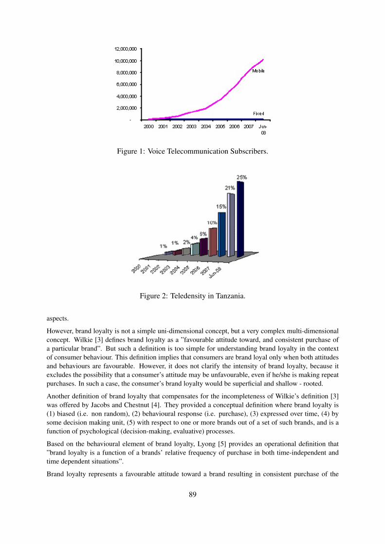
Figure 1: Voice Telecommunication Subscribers.

Figure 2: Teledensity in Tanzania.

aspects.

However, brand loyalty is not a simple uni-dimensional concept, but a very complex multi-dimensionalconcept. Wilkie [3] defines brand loyalty as a ”favourable attitude toward, and consistent purchase ofa particular brand”. But such a definition is too simple for understanding brand loyalty in the contextof consumer behaviour. This definition implies that consumers are brand loyal only when both attitudesand behaviours are favourable. However, it does not clarify the intensity of brand loyalty, because itexcludes the possibility that a consumer’s attitude may be unfavourable, even if he/she is making repeatpurchases. In such a case, the consumer’s brand loyalty would be superficial and shallow - rooted.

Another definition of brand loyalty that compensates for the incompleteness of Wilkie’s definition [3]was offered by Jacobs and Chestnut [4]. They provided a conceptual definition where brand loyalty is(1) biased (i.e. non random), (2) behavioural response (i.e. purchase), (3) expressed over time, (4) bysome decision making unit, (5) with respect to one or more brands out of a set of such brands, and is afunction of psychological (decision-making, evaluative) processes.

Based on the behavioural element of brand loyalty, Lyong [5] provides an operational definition that”brand loyalty is a function of a brands’ relative frequency of purchase in both time-independent andtime dependent situations”.

Brand loyalty represents a favourable attitude toward a brand resulting in consistent purchase of the

89

brand over time [6]. Two approaches to the study of brand loyalty have dominated marketing literature.The first is an instrumental conditioning approach, that views consistent purchasing of one brand overtime as an indication of brand loyalty. Repeat purchasing behaviour is assumed to reflect reinforcementand a strong stimulus-to-response link. The research that takes this approach uses probabilistic modelsof consumer learning to estimate the probability of a consumer buying the same brand again, given anumber of past purchases of that brand. This is a stochastic model rather than a deterministic model ofconsumer behaviour, as it does not predict one specific course of action. Rather, the prediction is alwaysin probability terms.

The second approach to the study of brand loyalty is based on cognitive theories. Some researchersbelieve that behaviour alone does not reflect brand loyalty. Loyalty implies a commitment to a brandthat may not be reflected by just measuring continuous behaviour.

Several authors have made distinctions between brand loyalty (in terms of repeat purchasing), and brandcommitment (implying some degree of high involvement). The brand loyalty that is defined here is theobserved behaviour of repeat purchasing of the same brand.

Behavioural measures have defined loyalty by the sequence of purchases (purchased Brand A give timesin a row) and/or the proportion of purchases, in the event that the customer is satisfied with the brandpurchase and repeats it in a relatively short period of time [7].

In order for managers to cope with the forces of disloyalty among consumers, there is a need to have anaccurate method to measure and predict brand loyalty. However it was impossible to obtain an objectiveand general measurement of brand loyalty, because brand loyalty has been defined in many differentways and operationalized by a number of scholars. The diverse definition and operationalization ofbrand loyalty in the past has been due to the various aspects of brand loyalty (e.g. behavioural andattitudinal brand loyalty).

A transition matrix was used as a forecasting instrument for determining the market environment in thefuture by Stan and Smith in a research conducted in 1964. This paper shows the potential of usingMarkov Chains in determining the intensive transitional probabilities for a new product. These proba-bilities may help marketing management by comparing the intensiveness gained in a certain period oftime with product life cycle. Thereby it may be possible to take the situation under control by takingcorrective action.

Although the Markov Chains Method is quite successful in forecasting (predicting) brand switching, thismodel still has some limitations:

1. Customers do not always buy products in certain intervals and they do not always buy the sameamount of a certain product. This means that in the future, two or more brands may be bought atthe same time.

2. Customers always enter and leave markets, and therefore markets are never stable.

3. The transition probabilities of a customer switching from an i brand to an j brand are not constantfor all customers, these probabilities may change from customer to customer and from time totime. These transitional probabilities may change according to the average time between buyingsituations.

4. The time between different buying situations may be a function of the last brand bought.

5. The other areas of the marketing environment such as sales promotions, advertising, competitionetc. were not included in these models.

90

3. Markov Chains MethodThe basic concepts of Markov Chains Method has been introduced by the Russian mathematician, An-drey Andreyevich Markov, in 1970. After this date many mathematicians have conducted research onMarkov Matrix and has helped it to develop. Markov Chains Method is used intensively for researchconducted on such social topics as the brand selection of customers, income distribution, immigrationas a geographic structure, and the occupational mobility (for examples and references please see [8],[9], [10]). In marketing, Markov Chains Model is frequently used for topics such as ”brand loyalty”and ”brand switching dynamics”. Although it is very complicated to transform marketing problems into mathematical equations, Markov Chains Method comes out as the primary and most powerful tech-nique in predicting the market share a product will achieve in the long term especially in an oligopolisticenvironment and in finding out the brand loyalty for a product.

The stochastic process is defined as a set of random variables Xt where the unit time parameter tis taken from a given set T . All the special values the random variables take on are named as a state.Therefore, a state variable name is given to theXt random variable. The set that accepts eachXt randomvariable is called an ”example space” or a ”state space”. If the S state space includes whole numberdiscontinuous values then it is called a stochastic process that is separate stated and these separate statedspaces may be countable and finite or countable and infinite. If Xt is defined in the t ∈ (−∞,∞)interval it is classified as a stochastic process that is real valued. Being a special type of stochasticprocess, the Markov Chain,

P (Xt+1 = xt|X0 = x0, X1 = x1, ..., Xt = xt) = P (Xt+1 = xt+1|Xt = xt); (t = 0, 1, 2, ...)

is a chain that has Markovian property and the Markovian property stresses that given the present (orpreceding) state, the conditional probability of the next state is independent of the preceding states.P (Xt+1 = xt+1|Xt = xt) are conditional probabilities and are named as transitional probabilities.

If the relationship

P (Xt+1 = xt+1|Xt = xt) = P (X1 = Xt+1|X0 = xt); (t = 0, 1, 2, ...)

exists, the one step transitional probabilities are usually shown as Pij and named as stationary and thetransitional probabilities that have this property do not change in time and the relationship

P (Xt+n = xt+1|Xt = xt) = P (Xn = xt+1|X0 = xt); (n = 0, 1, 2, ...)

becomes valid. These conditional probabilities are named as n-step transitional probabilities and areshown as Pnij . P

nij explains that the process that is in the i state, will be in the j state n steps later. This is

because Pnij are conditional probabilities and must be non-negative and also the relationship given belowis valid.

Σmj=1P

(n)ij = 1 ; i = 1, 2, ..., n = 0, 1, 2, ....

At this point n-step transitional probabilities matrix, S = S0, S1, ...., Sm state space may be shown as

P (n) =

S0 S1 . . . Sm

S0 P(n)00 P

(n)01 . . . P

(n)0m

S1 P(n)10 P

(n)11 . . . P

(n)1m

......

.... . .

...Sm P

(n)m0 P

(n)1m . . . P

(n)mm

91

If n = 1 is taken, then a stochastic process is a Markov Chain that has Markovian properties’. In thisresearch, only the Markov Chains that are finite and have stationary transitional probabilities will beconsidered.

4. Chapman - Kolmogorov EquationsThe P (n)

ij n-stepped transitional probabilities stress the probability of transition from the i state to the jstate at the n(> 1) step. The Chapman -Kolmogorov equations,

P(n)ij = Σm

k=oPikP(n−1)kj ∀ij and 0 ≤ m ≤ n

helps in forming a method for calculating the n-step transitional probabilities. In the special occasionswhere m = 1 and m = n− 1, the equations

P(n)ij = Σm

k=oPikP(n−1)kj ; (∀ij and n) and P

(n)ij = Σm

k=oP(n−1)ik Pkj

are obtained. These equations stress the fact that the n-step transitional probabilities may be calculatedfrom the one step transitional probabilities. For example, for n = 2

P(2)ij = Σm

k=oPikPkj

is obtained and a P 2ij are the elements of the P 2 matrix. P 2 is obtained from the multiplication of P by

P . Therefore, the n-step probabilities matrix may be calculated from the

Pn = P ∗ · P (n−1) = P (n−1) · P

relationship.

5. The long-term Behaviour of the Markov ChainThe ergodic chain (matrix) is defined as a chain where from one state it is possible to transform into allother states and where it contains no zero element that is at the powers of the P regular chain (matrix).Therefore it can be concluded that a regular matrix is ergodic but the opposite is not true. For the casewhere a T matrix is obtained by P having sufficiently big powers, if all of the line vectors of this Tmatrix are the same, it could be said that the P transitional matrix reaches a balance and there exists abalancing vector. A regular Markov Chain contains a single balance vector.

If v = [v1, v2, · · · vm] is a probability vector, then the relationship vp = v is valid and v is named as abalance vector.

6. Research MethodologyThe purpose of this study was to examine the cell phone users loyalty using the Markov Chains Method.For this study data has been collected for cell phone users loyalty for 400 subscribers from ten out oftwenty seven wards of Kinondoni District in Dar es salaam, Tanzania.For the purpose of this study, seven states were considered which stand for the network operators repre-sented in the form of a set as follows:

S = tiGO, Zantel, Vodacom, Airtel, Sasatel, Benson on Line, TTCLMobile

The data from the interviews was used to study cell phone users loyalty in two corresponding periods.

Following the two months interval, the switching behaviour of customers as well as their likelihood toexist in a given state was studied and the results were summarised in tabular form. The obtained results

92

Table 3: The transition results showing customers behaviour from July - August 2010NETWORK Vodacom tiGO Airtel Zantel TTCLMobile Total

Vodacom 60 2 0 0 0 62tiGO 3 288 2 0 0 293Airtel 0 0 34 0 0 34Zantel 0 0 0 9 0 9

TTCLMobile 0 0 0 0 2 2Total 63 290 36 9 2 400

shown in Tables 3 up to 8 were used to verify the hypothesis that cell phone users loyalty can be analysedusing Ergodic Transition Probability Matrices.

From Table 3, the sixth and seventh states, which stand for Benson on line and Sasatel companies, wereassumed to be redundant states because the results show that there were no chances for customers toexist into those states. As a result a reduced table made up of five states was obtained.

In addition, the non communicating states (also known as dominant states) were abandoned in the searchfor an Ergodic transition matrix. Table 4 is the transition probability matrix obtained from Table 3 afterremoving the dominant states.

Table 4: The transition Probability Matrix from July to August, 2010NETWORK Vodacom tiGO Airtel Total

Vodacom 0.9677 0.0323 0.0000 1.0000tiGO 0.0102 0.9829 0.0068 1.0000Airtel 0.0000 0.0000 1.0000 1.0000

The Transition probability matrix in Table 4 above is not Ergodic as it violates the condition of ergodicity[14], [15] hence it was not used in the analysis.

The transitions from September to October 2010 are summarized in Table 5.

Table 5: The transition results showing customers behaviour from September - October 2010NETWORK Vodacom tiGO Airtel Total

Vodacom 58 1 1 60tiGO 1 290 2 293Airtel 0 0 36 36Total 59 291 39 389

From Table 5 the following transition probability matrix was obtain.

The transition probability matrix in Table 6 above could not be used in the analysis of cell phone usersloyalty due to the existence of the dominant state Airtel. Customers switching behavior for the periodfrom November to December 2010 were summarized in Table 7.

From Table 7 the following transition probability matrix was obtained. Up to this point TCCLMobilewas still acting as a dominant state so it was excluded in the construction of the following transitionprobability matrix:

The above table indicated that during this period cell phone users were loyal to tiGO, followed by Airtel,then Vodacom and lastly Zantel with probabilities 0.9732, 0.9697, 0.9310 and 0.8750 respectively.

93

Table 6: The transition Probability Matrix from September to October, 2010NETWORK Vodacom tiGO Airtel Total

Vodacom 0.9667 0.0167 0.0167 1.0000tiGO 0.0034 0.9898 0.0068 1.0000Airtel 0.0303 0.0000 1.0000 1.0000

Table 7: The transition results showing customers behaviour from November - December 2010NETWORK Vodacom tiGO Airtel Zantel Total

Vodacom 54 3 1 0 58tiGO 5 291 2 1 299Airtel 1 0 32 0 33Zantel 0 1 0 7 8Total 60 295 35 8 398

Finally the switching behavior of cell phone users for four months of January to April 2011 were ob-tained as summarized in Table 9 below: This was because the switching behaviors of cell phone usersfor the months of January to February showed close similarity to that of March to April 2011. AlsoTTCLMobile was still a dominant state.

Table 9: The transition results showing customers behaviour from January - April 2011NETWORK Vodacom tiGO Airtel Zantel Total

Vodacom 46 12 2 0 60tiGO 4 284 7 0 295Airtel 1 6 28 0 35Zantel 0 2 0 6 8Total 51 304 37 6 398

The transition probability matrix constructed from Table 9 is as follows:

From Table 10 it was found that the leading company in terms of likelihood of having loyal customerswas respectively tiGo, Airtel, Vodacom, and lastly Zantel with probabilities 0.9627, 0.8000, 0.7667 and0.7500 respectively. The results in Table 10 shows only the existing situation of customer preferences,but the future stand or the long run forecast of the cell phone users distribution was analyzed by applyingthe Chapman-Kolmogorov equation.

7. Steady State Probability VectorMATLAB software was used in conjunction with the Chapman-Kolmogorov equation to perform itera-tions on the transition probability matrix obtained from July, 2010 to April, 2011. The analysis resultedin a steady state probability matrix called the stability situation. This result was obtained after 44 iter-ations which is equivalent to 7 years and 4 months. This result verified the hypothesis that a stabilizedErgodic Transition Probability Matrix plays a significant role in determining the steady state probabilityvector shown in table 11 below:

From Table 11 the results show that if things continue as they are now in the long run the most preferrednetwork company will be tiGO with the probability of 0.8297. The next preferred network will be Airtelwith the probability of 0.1086. Then Vodacom will follow with probability of 0.0617. Finally Zantelwill lose all its customers.

94

Table 8: The transition Probability Matrix from November to December, 2010NETWORK Vodacom tiGO Airtel Zantel Total

Vodacom 0.9310 0.0517 0.0172 0.0000 1.0000tiGO 0.0167 0.9732 0.0067 0.0033 1.0000Airtel 0.0303 0.0000 0.9697 0.0000 1.0000Zantel 0.0000 0.1250 0.0000 0.8750 1.0000

Table 10: The transition Probability Matrix from December, 2010 to April 2011NETWORK Vodacom tiGO Airtel Zantel Total

Vodacom 0.7667 0.2000 0.0333 0.0000 1.0000tiGO 0.0136 0.9627 0.0237 0.0000 1.0000Airtel 0.0286 0.1714 0.8000 0.0000 1.0000Zantel 0.0000 0.2500 0.0000 0.7500 1.0000

Finally the graphical analysis was done and the general network - customer status show that for theperiod from July 2010 to April 2011, the leading network was tiGO followed in descending order byVodacom, Airtel, Zantel, and lastly TTCLMobile as seen in the following figure:

Figure 3: The data for the graph were collected from Kinondoni District.

8. ConclusionAccording to the results discussed above, it was observed that Transition Probability Matrix for theperiods from July to August 2010 and September to October 2010 shown in Table ?? and 4 were notErgodic due to the existence of the absorbing state (i.e. the switching from Airtel to Airtel). On contrary,for the periods December 2010 to January 2011 the Transition probability Matrices were Ergodic andthe analysis from these matrices showed that cell phone users were loyal to tiGo network followed byAirtel then Vodacom and finally Zantel.

The graphical analysis shown in Figure 1 reveals that the number of cell phone users loyal to tiGO issignificantly larger than those loyal to Vodacom, Airtel Zantel and TTCLMobile. However in April 2011customers loyal to Airtel company seemed to approach those loyal to Vodacom, indicating the existenceof customer competition among the two networks.

95

Table 11: The steady state probability vectorNETWORK OPERATOR PROBABILITY

tiGO 0.8297Airtel 0.1086

Vodacom 0.0617Zantel 0.0000

The steady state vector computed from the Ergodic transition probability matrix using the Chapman-Kolmongorov equation revealed that in the long run tiGo network company will have a large share withabout 82.56 percent of cell phone users, followed by Airtel and Vodacom with 11.27 percent and 6.17percent respectively. On the other hand, the predictions show that Zantel network is going to lose all itscustomers and may go out of business.

9. RecommendationsThe results and conclusions above were based on a small sample of 400 cell phone users in KinondoniDistrict. The reasons for using such a small sample were lack of time and budgetary constraints. Werecommend that a study using a large sample from a large area of Tanzania should be done to get morereliable results. In fact, instead of using a two months interval a six months interval could be used.

Further studies should be done to analyze customers loyalty to other companies in Tanzania such asinsurance companies, banks etc. Another potential area where such analysis can play a significant roleis investigating the long time voters loyalty to current political parties in Tanzania to see which willsurvive and which are likely to die out.

References[1] Dick, A. S. , Basu, K. (1994), Consumer Loyalty: toward an integrated conceptual framework,

Journal of Academy of Marketing Science, Vol. 22, No. 2, p. 99-113.

[2] Kahn, B. E., Kalwani, M. U.; Morrison, D. G. (1986), Measuring Variety Seeking and Reinforce-ment Behaviours Using Panel Data, Journal of Marketing Research, Vol. 23, May, p. 89-100.

[3] Wilkie, W. L., (1994), Consumer Behaviour, John Wiley and Sons, New York.

[4] Jacoby, J. And Chestnut, R. W.(1978), Brand Loyalty: Measurement and Management, John Wileyand Sons, New York.

[5] Lyong Ha, Choong (1998), The Theory of Research Action Applied Brand Loyalty, Journal ofProduct and Brand Management, Vol. 7, Issue 1.

[6] Assael, Henry (1992), Consumer Behaviour and Marketing Action, Fourth Edition, PWS-KENTPublishing Company.

[7] Charnatony, Leslie de; McDonald, Malcolm H. B. (1992), Creating Powerful Brands, Butte worth-Heinemann Ltd., Linacre House, Jourdan Hill, Oxford.

[8] Frydman, H. (1984), Maximum Likelihood Estimation in the Moverstayer Model, Journal of theAmerican Statistical Association, 79, p. 632-638.

96

[9] Geweke, J. Marshall, R., Zarkin, G. (1986), ”Mobility Indices in Continuous Time Markov Chains,Econometrica, 54, p. 1407-1423.

[10] Simper, B., Spilerman, S. (1976), Some Methodological Issues in the Analysis of LongitudinalSurveys, Annals of Economic and Social Measurement, 5, 447- 474.

[11] Mtenzi, F. J., Chachage, B. L., Ngumbike F. ”The Growth of Tanzania Mobile Phone Sector:Triumph of Quantity, Failure of Quality” Proceedings of M4D, Karlstad University Sweden, p. 55- 61

[12] Tanzania Communication Regulatory Authority (2008) Market Statistics: TelecommunicationAvailable at http://www.tcra.go.tz/market%20info/statsTelecom.html

[13] Hisali, E. (2007) Review of Sector Taxation Policies and Determining the Elasticity of Penetra-tion and Price of the Various Telecommunication commissions Services in Uganda Available athttp://www.ucc.co.ug/

[14] Karlin S. and Taylor H. M. (1975) A First Course in Stochastic Processes 2nd Edition, AcademicPress Inc., New York

[15] Stone C. J., Hoel P. G. and Part S. C. (1972) Introduction to Stochastic Processes Houghton Mif-fling Company, Los Angeles.

97

Derivatives over Certain Finite Ringsby

Soud K. Mohamed

University of Dodoma, Tanzania

Abstract

We introduce a derivative of a relation over the ring of integers modulo an odd numberwhich is base on the very fundamental concepts which helped in the evolution of derivativeof a function over the real number field, namely slope. Then, for a prime field GF (p), weuse the derivatives to construct an algorithm that find all the directions, in the sense of [9],of graphs of certain exponential relations over R.

1. IntroductionDerivatives plays a very fundamental role in the analysis of functions over the real and the complexnumber fields. In these fields, their properties and applications are well-studied, since they reflect wellon our every day lives. Over finite rings the notion of a derivative first appeared some 75 year ago in thepaper [7] by H. Hasse. This derivative is the so called Hasse derivative, and has been successfully usedin areas where finite fields play an important role, such as Coding Theory [8].

Suppose that R is a commutative ring and let f(x) =∑n

i=0 aixi be a polynomial over R. Then the

rth-Hasse derivative of f(x) is f [r](x) =∑n

i=0 ( ir ) aixi−r with ( ir ) = 0 for i < r. It is well-known

that over a finite field K all functions are polynomial. In fact, if |K| = m, then there are mm functionsover K. In addition, there is a 1-1 correspondence between a function f : K → K and polynomial ofdegree less than m. So with Hasse derivatives one has every thing as far as a derivative of a functionover K.

If R is a finite commutative ring, then only a fraction of functions on R are polynomials [6]. So for afunction f on R which can not be represented by a polynomial over R, its Hasse derivative can not bedetermined. The aim of this paper is to introduce a derivative on a set of relations on certain rings.

Suppose that R is a finite ring and consider a relation ρ on R in a variable x, which shall be usuallydenoted by ρ(x). Then the image of ρ may sometimes be an array [10]. For instance, the image of afunction onR is an s×1-array. In Section 2 we will look into exponential relations and their arrays overthe ring R = Zn for an integer n, and then we give sufficient conditions for an exponential relation tobe a function over R.

Let R be the finite ring Zn, where n is an odd integer. Given a relation ρ, and a point a ∈ R, whatshould be the derivative of ρ at a? In real analysis we take the slope of a tangent line at a, provided itexists. Moreover for a relation on the real number fields, we have at lest one slope at a point: one along“each column” (picture the derivative of

√(x)). Over a finite field this is not possible, because a point

has more than one tangent! In addition, slopes of tangents can be computed along a column of ρ as wellas across it. In Section 3 we show that the slope of the “closest” secant to a point x ∈ R along a columnk is the “best candidate” for the derivative of ρ at x, which shall be denoted by Dr

(1)k (ρ(x)) or simply

ρ(1)k (x), the k-th derivative of ρ at x. This derivative has similar properties as the derivative of the real

number field, like: linearity; product and quotient rules and how it acts on polynomials and exponentialrelations. The definition of the derivative requires some ordering of the elements of R. In Section 1, weconsider the ring R as cyclically ordered set, which is very natural since R is a finite set.

98

Let R = Fq be a finite field with q elements and let ρ : R→ R be a relation. Define the set of directionsof ρ (slopes of secants of the graph of ρ) by:

D(ρ) :=

ρ(a)− ρ(b)

a− b| a 6= b ∈ R

(1.1)

The problem of determining the bound on the size ofD(ρ) has be studied extensively both geometricallyand combinatorically. The references [1], [3], [4] are some of the papers where this has been done.However, there has not been any attempt on computing the directions themselves, so far.

Given a graph of a column of a relation ρ over R, the size s of the graph is the number of elements inthe domain of ρ. Note that s is less than or equal to q. Now, ideally if one want to find all directions, onemay have to compute up to s(s− 1)/2 directions. The algorithm is as follow: you start at the first pointand then find s − 1 directions, then move to the second point and compute s − 2 directions, and so on.Since D(ρ) is a subset of R [3], there is a lot of unnecessary computations in this algorithm. In Section4 we show that for some relations ρ over prime fields, the derivatives of ρk is all one needs to find all thedirections of the graph of ρ.

2. PreliminariesIn this section we collect some of the preliminaries that will be needed in this paper. We fix the followingnotation: If R is a ring with unity, then R∗ will denote the group of units of R. Unless otherwisespecified,by order of an element a ∈ R we mean the multiplicative order of a.

2.1 Immediate successor and predecessor

Most “people” are very familiar with linear ordering. However, cyclic order is not a household term. Wegive a formal definition of cyclic order and use it to define some terminologies.

LetX be a set of at least 3 elements. A ternary relationC is a subset of the Cartesian productX×X×Xwhich satisfies the following axioms:

1. Cyclicity: if [a, b, c] is in C, then [b, c, a] is in C

2. Asymmetry: if [a, b, c] is in C, then [c, b, a] is not in C

3. Transitivity: if [a, b, c] and [a, c, d] are in C, then [a, b, d] is in C.

4. Totality or Completeness: if a, b and c are distinct, then either [a, b, c] is in C or [c, b, a] is in C.

If C satisfies the first three axioms, then it is called partial cyclic ordering on X , and consequently thepair (X,C) is a partially cyclically ordered set. If C satisfies all four axioms, it is called (total) cyclicordering on X , as a result we get cyclically ordered set (X,C).

If a cyclically ordered set X is finite of cardinality n, then there is a 1-1 correspondence between Xand the cyclically ordered set 1, 2, . . . , n, 1. We can use this correspondence to identify positionson X . Now, let X be a finite cyclically ordered set and let x ∈ X be at position i (using the abovecorrespondence), where i is an integer. Then the element in the position i+1 will be called an immediatesuccessor of x, and will be denoted by x+, while that in the position i − 1 will be called immediatepredecessor of x and will be denoted by x−.

2.2 Unity ordering

Let G be a finite group. The cyclic orderings on G which are of interest to us, are those that depend ongenerators of the group and the binary operation of the group. For example, for the additive group Z5,

99

we have the orderings 1, 2, 3, 4, 0, 3, 1, 4, 2, 0, 2, 4, 1, 3, 0 and 4, 3, 2, 1, 0, while for the multi-plicative group Z∗5 we have orderings 2, 4, 3, 1 and 3, 4, 2, 1. Given a generator g of a finite cyclicgroup, if the group is additive, then the ordering determined by g will be referred to g-additive cyclicordering, where as if the group is multiplicative, then the ordering will be referred to as g-multiplicativecyclic ordering

Suppose that G is a finite cyclically ordered group of order n ≥ 3 with a binary operation ∗. Then G hasat least one cyclic ordering, namely the one determined by each generator of G. For a, b ∈ G, define thelength from a to b, denoted by l(a, b), to be b ∗ a−1 ∈ G, where a−1 is the inverse of a. For example,in the cyclically ordered set Z5 = 0, 4, 3, 2, 1, we have that l(0, 3) = 3, l(2, 2) = 0, while for themultiplicative group Z∗5 = 1, 3, 4, 2 modulo 5 which is cyclically ordered, we have l(1, 3) = 3 andl(3, 2) = 4.

Now, for our group G above, we have that every element a ∈ G has an immediate predecessor andsuccessor. Then the length l(a, a+) will be referred to as the least length of a, and will be denoted byδ(a). For example, for multiplicative cyclically ordered group Z∗5 = 1, 2, 4, 3, we have that δ(x) = 3for all x ∈ Z∗5. The following fact can be easily proved.

Fact 2.25 Let R be a ring with unity 1R and isomorphic to the ring Zn.

i. For any additive ordering on R the least length δ(a) = δ is constant for all a ∈ R.

ii. There is an additive ordering on R such that δ(a) = δ = 1R

The cyclic ordering of Fact 2.25 (ii.) on a ring R will be called the unity ordering.

For the rest of the paper, we impose the following assumption on our ring R:

Assumption 1 R is the ring Zq where q is an odd integer. Moreover, the ordering onR is the associatedadditive cyclic ordering.

Remark 1 Under the above assumption our ring R will have a canonical cyclic ordering, which willbe fundamental throughout the paper. Moreover, no matter what additive cyclic ordering one takes onR, the element x+ − x− ∈ R will be a unit, since the ordering is determined by a generator of R.

3. Exponential and Hyperbolic Relations over RIn real analysis, exponential functions αx are very fundamental, and they can easily be used to defineother functions. Over finite ring, the mapping determined by αx, for a unit α, is not necessarily afunction. We have the following definition, which is motivated from [5].

Definition 3.26 Let α ∈ R be a unit of order N . Then, the exponential relation ρ : R → R is the rela-tion ρ(x) = αx. The image of ρ is anN×t-array [ρi(x)] with the a-th row, ρ(a) = αa, αa+q, . . . , αa+(t−1)q,where t ≤ N . The k-th column of ρ, ρk(x) = αx+kq, where x = 0, 1, . . . N − 1, will be called the k-thexponential relation of ρ.

Example 3.27 We consider examples:

1. Let R = Z7 and consider the relation ρ(x) = 2x mod 7. Then the array of ρ is

[ρk(x)] =

20 27 214 . . .21 28 215 · · ·22 29 216 · · ·

=

20 21 22

21 22 23

22 23 21

=

1 2 42 4 14 1 2

100

2. If R = Z9 and our relation is ρ(x) = 2x, then the array of ρ is

[ρk(x)] =

20 29 218 . . .21 210 219 · · ·22 211 220 · · ·23 212 221 · · ·24 213 222 · · ·25 214 223 · · ·

=

1 82 74 58 17 25 4

Computation of the array of the relation in Example 3.27 (1.) looks easy, because along columns androws one just increases the power by one. This is generally true for prime fields.

Lemma 3.28 If R is a prime field, and ρ(x) = αx is a relation on R, then the k-th relation of ρ isρk(x) = αx+k.

ProofWe have that kq mod N = kq−k+k mod N = k(q−1)+k mod N = k mod N , sinceN |q−1. Consider the relation ρ(x) = αx, where α ∈ R has order N . Then ρi(x) has N rows. However, asshown in the example above the number of columns may vary. If certain condition are satisfied, then thenumber of columns of the array of ρ can easily be obtained.

Theorem 3.29 Let α be a unit in R of order N , and let ρ(x) = αx be a relation.

(i) If a perfect square is not a factor of q and gcd(N, q) = 1, then [ρi(x)] is an N ×N -array.

(ii) If q = pm for a prime p, where m is a positive integer, then there are gcd(N, p − 1) columns in[ρi(x)].

ProofSuppose that [ρi(x)] is an s× t-array, and let the a-th row be ρ(a) = αa, αa+q, αa+2q, . . . , αa+(t−1)q.Then ρ(a) is a coset of the subgroup H = 〈αiq〉 of R∗ of order t. One can then observe that for bothcases, s = N and t ≤ N .

(i) Now αa = αa+tq means that tq = 0 mod N which is implies that N |tq. But since N does notdivide q, it must divide t. Hence t = N .

(ii) We have that H ≤ 〈α〉, since H contains power of α. Let K be a subgroup of R∗ of order p − 1.Since gcd(pn−1, p − 1) = 1, then R∗ ' Zpn−1 ⊕ Zp−1, and hence K is unique. From this we inferthat if β ∈ R∗ is such that βp−1 = 1, then β ∈ K. Now we have that (αiq)p−1 = (αφ(q))ip = 1 fori = 1, . . . t, so that H ≤ K. Hence t|N and t|p − 1, which implies that t ≤ gcd(N, p − 1) = d. Ifd < t, then αdq = αsNq+r(p−1)q = 1, so that |H| < t, a contradiction. The following corollary givesa sufficient condition for an exponential relation on R to be a function.

Corollary 3.30 Suppose that α ∈ R is unit of order N .

(i) If a perfect square is not a factor of q and N |q, then the relation ρ(x) = αx is a function.

(ii) If q = pm for a prime p and α has order pi for i = 1, . . .m− 1, then the relation ρ(x) = αx is afunction.

101

Proof(i) For all a ∈ R and some positive integer t, we have that ρ(a) = αa, αa+q, . . . , αa+(t−1)q = αa,since N |q.

(ii) Follows from Theorem 3.29, since gcd(pi, p− 1) = 1 for i = 1, . . .m− 1.

Let α ∈ R be a unit of order N , and consider the relation ρ(x) = αx. Then ρ is periodic of period N .More precisely, for a positive integer s each subset Sj = jN, jN+1, . . . , (j+1)N−1 of the domainof ρ, where j = 0, 1, . . . s − 1, determines the same image ρ(Sj) = ρ(jN), ρ(jN + 1), . . . , ρ((j +1)N − 1). The subset Sj is referred to as the j-th steps of ρ. As expected, starting at a point in R, thereare only a finite number of steps of ρ before one gets back to the same point.

Proposition 3.31 Let α ∈ R be a unit of order N , and consider the relation ρ(x) = αx. If gcd(N, q) =d, then ρ has q/d steps.

ProofLet ν be the least positive integer with the property that the set T = 0, N, 2N, . . . , (ν − 1)N takenmod q has distinct elements. Observe that find number of steps of ρ is the same as finding the cardinalityν of T . Also note that ν ≤ q/d. If ν > q/d, then |T | < ν, a contradiction.

Corollary 3.32 Let α ∈ R be a unit of order N , and consider the relation ρ(x) = αx. Then the mapπ = ρ|Sj

: Sj → im ρ is a permutation.

ProofOnly need to show that π is 1-1. Suppose that π(jN) = π(jN + k) for k 6= 0 mod N . ThenαjN = αjN+k which is equivalent to k = 0 mod N , a contradiction. We now define hyperbolicrelations over R.

Definition 3.33 Let α ∈ R be a unit of order N ≥ 3. Then

1. The k-th hyperbolic sine and cosine relations to the base α over R, denoted by sinhα,k(x) andsinhα,k(x) are respectively

coshα,k(x) :=αx+kq + α−(x+kq)

x+ − x−; sinhα,k(x) :=

αx+kq − α−(x+kq)

x+ − x−.

2. The hyperbolic since and cosine relations to the base α, denoted by coshα(x) and sinhα(x) arethe relations with images the N × t-arrays made by the columns coshα,k(x) and sinhα,k(x)respectively, where t < N .

Under certain assumption on R, hyperbolic relations on R behave like those over the real.

Proposition 3.34 Suppose that R has the unity ordering, and let α ∈ R be a unit of order N ≥ 3. Thenfor k = 0, 1, . . . N − 1:

(i) the identity cosh2α,k(x)− sinh2

α,k(x) = 1R holds,

(ii) coshα,k(−x) = coshα,k(x) and sinhα,k(−x) = − sinhα,k(x)

102

ProofFollows from the definition.

4. Derivatives and their PropertiesDenote the set of relations from R to R whose image are s× t-arrays by Relst(R) , and by Fun(R) theset of all functions from R to R.

Let q be the order of the ring R and let x ∈ R. For a positive integer k and a relation ρ ∈ Relst(R),define a map Dr

(1)k : Relst(R)→ Relst(R) on the k-th relation ρk of ρ by

Dr(1)k (ρ)(x) :=

ρk(x+ + kq)− ρk(x− + kq)

x+ − x−. (4.1)

If the context is clear, then Dr(1)k (ρ)(x) will be just denoted by ρ(1)

k (x).

If one looks closely at the this map one will notice that its value at a point x ∈ R is the slope of the“closest” secant to the point x along ρk. It can be also interpreted as the “average” of the two “closestslopes” to x along ρk. The result below show that the transformation has good properties too.

Theorem 4.35 Let ρ, γ ∈ Relst(R), x ∈ R and let c ∈ Z. Then

(i) the transformation Dr(1)k is linear.

(ii) Product Rule:

(ρkγk)(1)(x) = ρk(x− + kq)γ

(1)k (x) + γk(x+ + kq)f (1)(x)

= ρk(x+ + kq)γ(1)k (x) + γk(x− + kq)ρ

(1)k (x).

(iii) If γk(x) 6= 0 for all x ∈ R, then(ρkγk

)(1)

(x) =γk(x− + kq)ρ

(1)k (x)− ρk(x− + kq)γ

(1)k (x)

γk(x+ + kq)γk(x− + kq).

Proof(i) Follows easily.

(ii) We use the elementary “+- tricks”.

(ρkγk)(1)(x) =

(ρkγk)(x+ + kq)− (ρkγk)(x− + kq)

x+ − x−

=ρk(x+ + kq)γk(x+ + kq)− ρk(x− + kq)γk(x− + kq)

x+ − x−= ρk(x− + kq)γ

(1)k (x) + γk(x+ + kq)ρ

(1)k (x)

(iii) Exercise.

Remark 2 If R is a prime field, then (4.1) and its subsequent formulas in Theorem 4.35 become mucheasier, by the use of Lemma 3.28.

Example 4.36 Let us look into examples:

103

(i) Let p be an odd prime number and consider the ring Zp with the associated additive cyclic order-ing. Let f(x) = ax mod p. Then for each x ∈ Zp, δ(x) = 1 ∈ Zp, so that x+−x− = 2 is a unitin Zp. So, f (1)(x) = a(x+1)−a(x−1)

2 = a. For g(x) = bx2 mod p, we have that g(1)(x) = 2bx.

(ii) Let R = Z9 has the unity ordering, and consider the relation ρ ∈ Rel(R) given by ρ(x) =2x. Then the image of ρ is 6 × 2-array with columns ρ0(x) = 20, 21, 22, 23, 24, 24 andρ1(x) = 23, 24, 25, 20, 21, 22. One can verify that ρ(1)

0 (x) = 3, 6, 3, 6, 3, 6 and ρ(1)1 (x) =

6, 3, 6, 3, 6, 3 for x ∈ R.

(iii) Consider the ring Z35, and let R = 5Z35 = 0, 5, 10, 15, 20, 25, 30. Then R is a ring modulo35 whose unity 1R = 15. If one considers the given cyclic ordering on R, then for each x ∈ R,δ(x) = δ = 5 and x+ − x− = 2δ = 10 which is a unit in R. Consider the relation ρ(x) = 255x

mod 35 on R. Then the image of ρ is a 3 × 3-array, and we have that ρ(1)0 (x) = 25, 15, 30,

ρ(1)1 (x) = 15, 30, 25 and ρ(1)

2 (x) = 30, 25, 15 for x ∈ R.

The computation in Example 4.36 (i) and (ii) would not be very clear as far as ρ(1)k (0) is concerned. But

we used the following result.

Lemma 4.37 Suppose α ∈ R is a unit of order N ≥ 3, and let ρ(x) = αx be a relation on R.Then ρ(k) = ρ(sN + j), for all integers j, s. In particular, ρ(0) = ρ(N), ρ(−1) = ρ(N − 1) andρ(N + 1) = ρ(1)

ProofWe have that ρ(j) = αj = αsN+j = ρ(sN + j).

From the above theorem we see that the transformation ρ(1)k looks indeed like a derivative on Relst(R).

For, when applied to a constant function it vanishes, and when applied to a polynomial of degree two itgives a polynomial of degree one, and so on. Also, when the transformation is applied to an exponentialrelation over R, it produces the relation times a constant. The above behavior are similar to those seenin the derivative transformation of real functions.

Definition 4.38 Let ρ be a relation on R and let x ∈ R. If ρ(1)k (x) is defined, then it will be called the

k-th derivative of the relation ρ at x, and will be denoted by ρ(1)k (x).

In the real analysis case we are used to very nice derivative formulas for functions. The situation here isthe similar, and we have the following result.

Corollary 4.39 LetR has unity 1R and let δ be the least length. If α ∈ R is a unit and n is a nonnegativeinteger greater than 1, then

(i) (αx)(1)k (x) = (α2δ−1R)

2δαδαx+kq

(ii) (xn)(1)(x) =∑s

i=0 ( n2i+1 )xn−(2i+1)δ2i; s =

n2 − 1 n evenn−1

2 n odd

(iii) (sinhα,h(x))(1)(x) = (α2δ−1R)2δαδ

coshα,h(x)

(iv) (coshα,h(x))(1)(x) = (α2δ−1R)2δαδ

sinhα,h(x)

104

ProofOne just uses the definition of the derivative.

Remark 3 1. If the ordering of R in Corollary 4.39 is the unity ordering, then δ = 1R and the formulasbecome much simpler.

2. Theorem 4.35 and Corollary 4.39 can be used to find k-th derivatives of all relations which are linearcombinations or products of the set of k-th relations xn, αxk, sinhα,k(x), coshα,k(x) for a unit α ∈ R.

3. The derivative of a monomial function whose degree is divisible q is not zero in R.

The derivative is a linear transformation on Relst(R). So it can be applied on a relation ρmore that onceand still preserve the linearity property. The following result, which is a consequence of Theorem 4.35and Corollary 4.39, gives formulas for computing k-th derivatives of certain relations ρ, t times, whichwill be called (t, k)-th derivative of ρ. If the array of ρ has only one column, then the (t, 0)-th derivativewill be just called t-th derivative.

Corollary 4.40 Let α ∈ R be a unit, and let δ is the least length. Then for a nonnegative integer t:

(i)

(xn)(t)(x) =s∑i=0

( n2i+1 ) (xn−(2i+1))(t−1)(x)δ2i; s =

n2 − 1 n evenn−1

2 n odd

(ii) (αx)(t)k (x) = (α

2δ−1R2δαδ

)tαx+kq

Proof(i) Follows from (4.1) and Theorem 4.35.

(ii) Exercise. Over the real the derivative transformationis not necessarily periodic for exponential functions. Over prime fields the derivative transformation onan exponential relation is periodic for most of the bases.

Theorem 4.41 Let R = GF (q) for a prime number q, and let α ∈ R be a unit which is not a squareroot of unity. If ρ(x) = αx, then

ρ(t)h (x) = ρh(x) for some positive integer t

ProofBy the assumption α2 − 1 6= 0 ∈ R, so that α

2−12α ∈ R∗, which implies that (α

2−12α )t = 1 ∈ R∗ some

positive integer t.

4.1 “The Exponential Values e”

In real analysis the exponential relation exp(x) = ex is characterized by its derivative, in the sense thatit is the only relation with derivative equals the relation itself. Given a finite ring with additive cyclicallyordering, do we have an analog of the exponential relation with respect the derivative we have defined?The answer is not necessarily! But some rings have indeed got a pair of e’s. The result below gives asufficient condition for that to happen.

Theorem 4.42 Let R = GF (q), where q ≥ 3 is prime. If 2 is a quadratic residue in R, then theelements e = 1±

√2 has the property that ρ(1)

k (x) = ρk(x), where ρk is the k-th relation of the relationρ(x) = ex.

105

ProofConsider the relation ρ(x) = ex, where e is in R. Suppose that ρ(x) has the property that ρ(1)

k (x) =ρk(x) for all k. Then one has that e2 − 2e− 1 = 0 ∈ R, which means e = 1±

√2.

5. Finding DirectionsThroughout this section R = GF (q) for an odd prime q, and the ordering of R is the unity ordering.Recall that for a relation ρ : R → R, the set of directions of ρ is denoted by D(f) (see (1.1)). Let usdenote the set of all (i, k)-th derivatives of ρ by Dr

(i)k (ρ) i.e.

Dr(i)k (ρ) := ρ(i)

k (x) | x ∈ R (5.1)

From the definition of derivative we see that Dr(i)k (ρ) ⊆ D(ρ) for all i, k.

For a relation ρ : R → R, the bound on the size of D(ρ) has be well studied. But there are only fewrelations ρ over R whereby the exact size of D(ρ) is known. So far these are the known ones: linearfunctions f [|D(f)| = 1] (see [9]); functions f(x) = x(q+1)/2 [|D(f)| = (q+ 3)/2)] (see [3]). We willtry to add to this collection. We need the following lemma.

Lemma 5.43 Let α ∈ R be a unit of order N ≥ 3, and consider the relation ρ(x) = αx. Then for allx ∈ R, ρ(i)

k (x) 6= 0 ∈ R for all i, k.

ProofFor x ∈ R such that jN + 1 ≤ x ≤ (j + 1)N − 1, we have that ρ(i)

k (x) 6= 0 for all j, k, by Corollary3.32. One can easily verify that ρ(i)

k (jN) 6= 0, for all i, j, k. Suppose that α ∈ R is a unit, andlet ρ(x) = αx be a relation. Then by Theorem 4.41, applying the derivative transformation repeatedlygives back ρ(x). We have two cases for β = α2−1

2α :

Case 1: If β is in 〈α〉, then we get a permutation of 〈α〉 whose order it the order of subgroup generatedby β.

Case 2: If β is not in 〈α〉, then the collection Dr(i)k (ρ) partitions a bigger subgroup of R∗ containing

〈α〉. If this happens, then we say that α partitions the subgroup.

We have the following result.

Lemma 5.44 Let α be a unit in R, and let ρ(x) = αx be a relation. Then the order of Dr(i)k (ρ) divides

q − 1 for all i, k. In particular, if α is a generator of R∗, then |Dr(i)k (ρ)| = q − 1 for all i, k.

ProofWe know that the set Dr

(i)k (ρ) is a coset of 〈α〉 in R∗ for all i, k. Then the result follows, since all cosets

of a subgroup have the same size.

Now we have our main result of this section, which establishes a connection between D(ρ) and Dr(i)(ρ)for exponential relations ρ(x).

Theorem 5.45 Suppose that α is a unit in R of order N ≥ 3, consider the relation ρ(x) = αx, and lets be the order of α

2−12α .

(i) If α partitions R∗, then for all k

D(ρ) = Dr(1)k (ρ) tDr

(2)k (ρ) t · · · tDr

(s)k (ρ) t 0,

106

(ii) If α is a generator of R∗, then

D(ρ) = Dr(i)k (ρ) t 0 for all i, k.

Proof(i) Let T = Dr

(1)k (ρ) t Dr

(2)k (ρ) t · · · t Dr

(s)k (ρ). Then |T | = q − 1, since α partitions R∗. We also

have that 0 is not in Dr(i)k (ρ) for all i, k, by Lemma 5.43. Since Dr

(i)k (ρ) ⊆ D(ρ) and D(ρ) ≤ q for all

i, the result follows.

(ii) By Lemma 5.44 we have that |Dr(i)k (ρ)| = q−1 and 0 /∈ Dr

(i)k (ρ) by Lemma 5.43, for all i, k. Since

Dr(i)k (ρ) ⊂ D(ρ) for all i, k, and D(ρ) ≤ q, the result follows.

References[1] S. Ball (2003), The number of directions determined by a function over finite field J. Combin. Theory

Ser. A, 104 341-435.

[2] S. Ball (2007), Functions over finite fields that determine few directions, Electr. Notes in DiscreteMath., 29, 185-188.

[3] S. ball (2011) Lacunary Polynomials over Finite Fields, Preprint.

[4] A. Blockhuis, S. Ball, A. E. Brouwer, L. Storme and T. Szonyi (1999) On the number of slopes ofthe graph of a function defined on a finite field, J. Combin. Theory Ser. A, 86 187-196.

[5] R. M. Campello de Souza, H. M. de Oliveira, A. N. Kauffman, A. J. A. Paschoal (1998), Trigonom-etry in finite fields and a new Hartley transform, ISIT 1998, Cambridge, MA, USA.

[6] S. Frisch (1999), Polynomial fuctions on finite commutative rings, Lec. Notes in Pure and Appl.Maths 205, Dekker, 323-336.

[7] H. Hasse (1936), Theorie der hoheren Differentiale in einem algebraischen Funktionenkorper mitvollkommenen Konstantenkorper bei beliebiger charakteristik, J. Reine Ang. Math., vol. 175, 50-54.

[8] J. L. Massey, N. von Seeman, P. Schoeller (1986), Hasse derivatives and repeated-root cyclic codes,IEEE Symposium of Info. Theory, Ann. Arbor, USA.

[9] L. Redei (1973), Luchenhafte Polynome uber endkichen Korper, Birkhauser-Verlag, Basel.

[10] M.M.C. de Souza, H.M. de Oliveira, R.M.C. de Souza, M.M. Vasconcelos (2004), The DiscreteCosine Transform over Prime Finite Fields, LNCS,Vol. 3124/2004, 37-59

107

Bifurcation results on symplectic manifoldsby

Eleonora Ciriza

Universita degli Studi di Roma Tor Vergata, Italy

1. IntroductionExistence and multiplicity of periodic trajectories of Hamiltonian vector fields on symplectic manifoldsis a traditional field of research, which found new input from the work on Arnold’s conjecture. Fitz-patrick, Pejsachowicz and Recht in [8],[9] studied bifurcation of periodic solutions of one-parameterfamilies of (time dependent) periodic Hamiltonian systems in R2n relating the spectral flow to the bi-furcation of critical points of strongly indefinite functionals.

In [6] we extended their results to families of time dependent Hamiltonian vector fields acting on sym-plectic manifolds and the related problems of bifurcation of fixed points of one parameter families ofsymplectomorphisms were discussed. Namely we proved that for a 1-parameter family of time depen-dent Hamiltonian vector fields, acting on a symplectic manifold M which possesses a known trivialbranch uλ of 1-periodic solutions if the relative Conley Zehnder index of the monodromy path alonguλ(0) is defined and does not vanish then any neighborhood of the trivial branch contains 1-periodicsolutions not in the branch.

Fixed points of Hamiltonian symplectomorphisms are in one to one correspondence with 1-periodicorbits of the corresponding vector field. Hence as a consequence we obtained, assuming that (M,ω)is a closed symplectic manifold with trivial first De Rham cohomology group, for a path φ : [0, 1] →Symp0(M) of symplectomorphisms with a known smooth path p : [0, 1]→ U of fixed points, i.e. , p(λ)is a fixed point of φλ. If the Conley-Zehnder index CZ(φ, p) of φ along p is defined and does not vanishthen there is a bifurcation of fixed points of φ from the trivial branch p.

The Arnold conjecture states that a generic Hamiltonian symplectomorphism has more fixed points thatcould be predicted from the fixed point index. More precisely, by the fixed point theory a diffeomorphismisotopic to the identity with non-degenerate fixed points must have at least as many fixed points asthe Euler-Poincare characteristic of the manifold. But the number of fixed points of a Hamiltoniansymplectomorphism verifying the same non-degeneracy assumptions is bounded bellow by the sum ofthe Betti numbers. Roughly speaking, this can be explained by the presence of a variational structure inthe problem. Fixed points viewed as periodic orbits of the corresponding vector field are critical pointsof the action functional either if the orbits are contractible or when the symplectic form is exact.

Applied to bifurcation of fixed points of one parameter families of Hamiltonian symplectomorphismsour result shows a similar influence on the presence of a variational structure. In order to see the analogyconsider a one parameter family of diffeomorphisms ψλ;λ ∈ [0, 1] of an oriented manifoldM , assumingfor simplicity that ψλ(p) = p and that p is a non degenerate fixed point of ψi; i = 0, 1. The work of Ize[11] implies that the only homotopy invariant determining the bifurcation of fixed points in terms of thefamily of linearizations L ≡ Tpψλ at p is given by the parity

π(L) = sign det(Tpψ0) · sign det(Tpψ1) ∈ Z2 = 1,−1.

Here det is the determinant of an endomorphism of the oriented vector space TpM . In other wordsbifurcation arise whenever the det(Tpψλ) change sign at the end points of the interval. Moreover, anyfamily of diffeomorphisms close enough to ψ in the C1-topology and having p as fixed point undergoesbifurcation as well. On the contrary if both sign coincide one can find a perturbation as above withno bifurcation points at all. The integer valued Conley-Zehnder index provides a stronger bifurcation

108

invariant for one parameter families of Hamiltonian symplectomorphisms. It forces bifurcation of fixedpoints whenever the Conley-Zehnder index CZ(L) is non zero even when π(L) = 1. The relationbetween the two invariants is π(L) = (−1)CZ(L).

A natural generalization of the classical Arnold’s conjecture estimates the number of intersection pointsof two Lagrangian submanifolds of a symplectic manifold.

The cause that forces Hamiltonian deformation L1 = φ(L) of a compact Lagrangian submanifold L ofM to have a huge intersection withL can be explained as follows: by a well known theorem of Weinsteinthe submanifold L has a neighborhood symplectomorphic to a neighborhood of the zero section in thecotangent bundle T ∗(L). If L is simply connected and if L1 is a Lagrangian submanifold that is C1

close to L then L1 is given by the image of the differential dS : L → T ∗(L) of a smooth functionS : L → R2n and therefore will have as many intersection points with L as critical points has thefunction S on L. The latter is bounded from below by Lusternik-Schnirelmann inequalities or by Morseinequalities if the critical points are non-degenerate. Of course L1 need not be C1-close to L. But whenM = T ∗(N) using an Hamiltonian isotopy φλ with φ1 = φ one can still produce a family of generatingfunctions S : N ×Rk → R with k big enough such that critical points of S correspond to intersectionsof N with L1. This is a Theorem of Sikorav [18]. Using this theorem one can still get estimates on thenumber of intersection points but weaker than in the previous case. Functions S as before are usuallycalled generating families.

In [7] we showed that intersections of one parameter families of Lagrangian submanifolds with a givenone have stronger bifurcation properties than the intersections of general submanifolds of right codi-mension essentially for the same reason as above. For families Lλ close enough in the C1 topology to agiven Lagrangian submanifold L0 bifurcation of intersection points of Lλ with L0 reduces, by the abovedescribed process, to bifurcation of critical points of one parameter families of smooth functions. Inthis setting bifurcation arises whenever the spectral flow, or what is the same, the difference between theMorse indexes of the end points of the trivial branch is non-zero. This gives a stronger invariant than theusual bifurcation index obtained by comparing the sign of the determinant of the Jacobian matrix of thegradient at the end points of the trivial branch. Via generating functions we showed that the assumptionof being C1 close can be substituted with a more general one without modifying the conclusions.

Namely the main result in [7] is as follows. Let N be a closed manifold and let L = Lλ be an exact,compactly supported family of Lagrangian submanifolds of the symplectic manifold M = T ∗(N) suchthat L0 admits a generating family quadratic at infinity. Let p : [0, 1] → M be a path of intersectionpoints of Lλ with N . Assume that Lλ is transversal to N at p(λ) for λ = 0, 1 and that the Maslovintersection index µ(L,N ; p) is different from zero. Then arbitrarily close to the branch p there areintersection points of Lλ with N such that do not belong to p.

The results exposed here were obtained in collaboration with J. Pejsachowicz. Symplectic featuresnedeed for our purpose are collected in section §2. In section §3 we extend the definitions of the Maslovand Conley-Zehnder indeces to manifolds. This relies on the existence of symplectic trivializations ofsymplectic vector bundles over an interval. In §4 we outline how the bifurcation results of Fitzpatrick,Pejsachowicz and Recht are applied to the situations described above.

I would like to thank Ramadas Ramakrishnan from ICTP and the EAUMP’s coordinators John Mango,Egbert Mujuni, Sylvester Rugeihyamu for inviting me to take part on the EAUMP project. I also wishto thank Velleda Baldoni for finantial support.

2. Symplectic featuresA symplectic manifold M is a differentiable manifold together with a closed nondegenerate differen-

109

tiable two form ω, i.e. ,

dω = 0 and ∀Y 6= 0 ∃X : ω(X,Y ) 6= 0, X, Y ∈ TmM.

HenceM must have even dimension and because ωn/n! gives the canonical volumen form it is oriented.

The non-degeneracy condition induces an isomorphism between the tangent T (M) and the cotangentspace of the manifold T ∗(M) that assigns to each vector field X a 1-form ιXω = ω(X, .).

A diffeomorphism φ : (M,ω) → (M,ω) that satisfies φ∗ω = ω is called symplectomorphism. Inparticular, a simplectomorphism preserves the volumen.

The requirement on the 2-form ω to be closed provides a correspondence between closed 1-forms andconservative vector fields since in this case LXω = 0 if and only if d(ιXω) = 0, such vector fields arecalled symplectic. The flow generated by a symplectic vector field consist of symplectomorphisms, i.e. ,φ∗tω = ω ∀t. A vector field is called Hamiltonian if the 1-form ιXω is exact.

Because on a manifold there are many 1-forms the dimension of the group of symplectomorphisms ofM , Symp(M,ω) is infinity. To the subset of exact 1-forms α = dH corresponds a normal subgroupHam(M,ω) of Symp(M,ω).

In symplectic geometry there are no local invariants like for instance the curvature in Riemannian ge-ometry. Darboux Theorem states that in some neighborhood of a given point one can choose a coor-dinate system (U ;x1, . . . xn, y1, . . . , yn) such that the restriction of the form to the neighborhood U isω|U = ω0 :=

∑ni=1 dxi ∧ dyi. Hence the universal local model of a symplectic form is the standard

symplectic form ω0 in R2n. In this case the isomorphism between the tangent and cotangent space isgiven explicity by X = ∂/∂xj → ιXω0 = dyj , X = ∂/∂yj → ιXω0 = −dxj .

An important example of symplectic manifolds is the cotangent bundle of any manifold. Let N be ann-dimensional differentiable manifold. Let T ∗(N) be the cotangent bundle of N and π : T ∗N → N theprojection on N . There is a canonical 1-form λN on T ∗N defined as follows: let ξ be a tangent vectorto T ∗N at the point p ∈ T ∗N (ξ ∈ Tp(T ∗(N))). Since the element p is a cotangent vector on Tx(N)where x = π(p) and π∗(ξ) ∈ Tx(N) define λN (ξ) := p(π∗(ξ)). In local coordinates λN (ξ) = pdq andthe symplectic 2-form is Ω = dλN . Being exact it is closed and it is non-degenerate because in localcoordinates Ω = dp ∧ dq.

Let W be a vector subspace of a symplectic vector space (V, ω), the symplectic orthogonal to W is thevector subspace Wω := v ∈ V/ω(v, w) = 0 ∀v, w ∈ W. W is said to be isotropic if W ⊂ Wω. It issaid to be coisotropic if W ⊃Wω. If it is both isotropic and coisotropic it is called Lagrangian.

If W is isotropic, then Wω is coisotropic and the symplectic form ω induces a symplectic form $on the quotient space Wω/W defined by $(v + W,w + W ) = ω(v, w) ∀v, w ∈ Wω. The space(Wω/W,$) is called the isotropic redution. Moreover if L is a Lagrangian subspace of (V, ω) thenLW = (L ∩Wω)/(L ∩W ) is a Lagrangian subspace of Wω/W .

Lagrangian submanifolds of a symplectic manifold (M,ω) are the submanifolds of maximal dimensionwhere the symplectic form vanishes. They are characterized by TL = (TL)ω. Examples of Lagrangiansubmanifolds are the vertical fibers of a cotangent bundle T ∗N . As for submanifolds transverse to thefibers, any such submanifold is locally the graph of a 1-form α : N → T ∗N . The graph of a 1-form αis Lagrangian if and only if α is closed. If the 1-form is exact, i.e. , if α = dS the funtion S is called agenerating function for the corresponding submanifold.

Any Lagrangian submanifold can be generated locally by a function on the product of N with a para-menter space, in which case it is called generating family.

110

The definition goes as follows (see [21]). Let V be a finite dimensional vector space. Consider a smoothfunction S : N × V → R such that the differential dS is transversal to the submanifold

N0 = T ∗(N)× V × 0 of T ∗(N × V ) ≡ T ∗(N)× V × V

Denote by Sn the function Sn : V → R defined by Sn(v) = S(n, v) and by Sv the function Sv : N → Rdefined by Sv(n) = S(n, v). By the implicit function theorem, the set C = (n, v)/dSn(v) = 0 ofvertical critical points of S is a submanifold of N × V of the same dimension as N .

Let e : C → T ∗(N) defined by e(n, v) = dSv(n). The map e is a Lagrangian immersion (but generallynot an embedding) of the manifold C into T ∗N . Given a Lagrangian submanifold L of T ∗(N), S is saidto be a generating family for L if there is a diffeomorphism h from C onto L such that e = ih, wherei : L→ T ∗(N) denotes the inclusion. The generating family S is said to be quadratic at infinity if thereis a non-degenerate quadratic form Q on V such that S(n, v) = Q(v) for ‖v‖ big enough.

Diffeomorphisms of a manifold may be identified with their graphs, that is, with submanifolds ofM×Mwhich are mapped diffeomorphically onto M by the projections π1, π2. If M carries a symplecticstructure ω, the form π∗1ω − π∗2ω defines a symplectic structure on the product manifold M ×M . Adiffeomorphism φ of a symplectic manifold (M,ω) is a symplectomorphism if and only if its graph is aLagrangian submanifold of (M ×M,π∗1ω − π∗2ω). Fixed points of φ correspond to intersections of thegraph with the diagonal ∆ of M ×M .

On a closed symplectic manifold (M2n, ω) every smooth time dependent (Hamiltonian) functionH : R×M → R gives rise to a family of time dependent Hamiltonian vector fields X : R×M → TM definedby

ω(X(t, x), ξ) = dxH(t, x)ξ

for ξ ∈ TxM . If H is periodic in time with period 1, then so is X . By compactness and periodicity thesolutions u(t) of the initial value problem for the Hamiltonian differential equation

ddtu(t) = X(t, u(t)),

u(s) = x(2.1)

are defined for all times t. The flow (or evolution map) associated to X is the two-parameter family ofsymplectomorphisms ψ : R2 → Symp(M) defined by

ψs,t(x) = u(t)

where u is the unique solution of (2.1).

By the uniqueness and smooth dependence on initial value theorems for solutions of differential equa-tions the map ψ : R2×M →M is smooth. The diffeomorphisms ψs,t verify the usual cocycle propertyof an evolution operator i .e. ,ψs,r ψr,t = ψs,t and ψt,t = Id . From this property it follows that foreach fixed s, the map sending u into u(s) is a bijection between the set of 1-periodic solutions of thetime dependent vector field X and the set of all fixed points of ψs,s+1. Hence in order to find periodictrajectories of (2.1) we can restrict our attention to the fixed points of P = ψ0,1. The map P = ψ0,1 iscalled the period or Poincare map of X.

A 1-periodic trajectory is called non degenerate if p = u(0) is a non degenerate fixed point of P ,i.e. , if the monodromy operator Sp ≡ TpP : TpM → TpM has no 1 as eigenvalue. Consistently, theeigenvalues of the monodromy operator will be called Floquet multipliers of the periodic trajectory.The particular choice of s = 0 is irrelevant to the property of being non degenerate since the Floquetmultipliers do not depend on this choice. (see [1])

111

Every symplectomorphism that can be represented as a time 1-map of such a time dependent Hamilto-nian flow is called a Hamiltonian map. IfM is simply connected the connected component of the identitymap Symp0(M,ω) in the space of symplectic diffeomorphisms Symp(M,ω) consists of Hamiltonianmaps (see [12]).

3. The Maslov index and the Conley-Zehnder indexBefore going to the manifold setting let us discuss the case of R2n = T ∗Rn with the standard symplecticform ω0 =

∑dxi ∧ dyi. The group of real 2n× 2n symplectic matrices will be denoted by Sp(2n,R).

The relative Conley-Zehnder index is a homotopy invariant associated to any pathψ : [0, 1]→ Sp(2n,R)of symplectic matrices with no eigenvectors corresponding to the eigenvalue 1 at the end points. Thisinvariant counts algebraically the number of parameters t in the open interval (0, 1) for which ψ(t) has1 as an eigenvalue. One of the possible constructions uses the Maslov index for non-closed paths. Weshall define it along the lines of Arnold [3] for closed paths. For an alternative construction see Robbinand Salamon [15].

The Lagrangian Grassmaniann Λ(n) consists of all Lagrangian subspaces of R2n considered as a topo-logical space with the topology it inherits as a subspace of the ordinary Grassmanian of n-planes. Let Jbe the selfadjoint endomorphism representing the form ω0 with respect to the standard scalar product inR2n. Namely, ω0(u, v) ≡< Ju, v >. Then J is a complex structure, it is indeed the standard one. Itcoincides with multiplication by i under the isomorphism sending (x, y) ∈ R2n into x + iy in Cn. Interms of this representation, a Lagrangian subspace is characterized by JL = L⊥.

Using the above description one can identify Λ(n) with the homogeneous space U(n)/O(n). Thiscan be done as follows: given any orthonormal basis of a Lagrangian subspace L there exist a uniqueunitary endomorphism A ∈ U(n) sending the canonical basis of L0 = Rn × 0 into the given oneand in particular sending L0 into L. Moreover the isotropy group of L0 can be easily identified withO(n). Hence we obtain a diffeomorphism between U(n)/O(n) and Λ(n) sending the class [A] intoA(L0). Since the determinant of an element in O(n) is ±1, the map sending A into the square of thedeterminant of A factorizes through Λ(n) ≡ U(n)/O(n) and hence induces a one form Θ ∈ Ω1

(Λ(n)

)given by Θ = [det2]∗θ, where θ ∈ Ω1(S1) is the standard angular form on the unit circle. This form iscalled the Keller-Maslov-Arnold form.

The Maslov index of a closed path γ in Λ(n) is the integer defined by µ(γ) =∫γ Θ. In other words µ(γ)

is the winding number of the closed curve t→ det2(γ(t)

). The Maslov index induces an isomorphism

between π1(Λ) and Z.

The construction can be extended to non-closed paths as follows: fix L ∈ Λ(n). If L′ is any Lagrangiansubspace transverse to L then L′ can be identified with the graph of a symmetric transformation fromJL into itself. It follows from this that the set ΛL of all Lagrangian subspaces L′ transverse to L is anaffine space diffeomorphic to the space of all symmetric forms on Rn and hence it is contractible.

We shall say that a path in Λ(n) is admissible with respect to L if the end points of the path are transverseto L. The Maslov index µ(γ, L) of an admissible path γ with respect to L is defined as follows: takeany path δ in ΛL joining the end points of γ and define

µ(γ;L) ≡ µ(γ′) =

∫γ′

Θ.

where γ′ is the path γ followed by δ. The result is independent of the choice of δ. Moreover, since ΛLis contractible, µ(γ;L) is invariant under homotopies keeping the end points in ΛL.

Geometricaly, the Maslov index µ(γ;L) can be interpreted as an intersection index of the path γ with theone codimensional analytic set Σl = Λ(n)−ΛL (see [16]). From the definition it follows that the index

112

is additive under concatenation of paths. Namely, given two admissible paths α and β with α(1) = β(0)

µ(α ? β;L) = µ(α;L) + µ(β;L).

Since Sp(2n,R) is connected it follows from the homotopy invariance that

µ(Sγ;SL) = µ(γ;L)

for any symplectic isomorphism S. This allows to extend the notion of Maslov Index to paths of La-grangian subspaces in Λ(V ), where (V, ω) is any finite dimensional symplectic vector space.

Graphs of symplectic endomorphisms are Lagrangian subspaces of the symplectic vector space V × Vendowed with the symplectic form ω×(−ω). The graph of P ∈ Sp(2n,R) is transversal to the diagonal∆ ⊂ V × V if and only if 1 is not an eigenvalue of P . A path φ : [0, 1] → Sp(2n,R) will be calledadmissible if 1 is not in the spectrum of its end points. For such a path the relative Conley-Zehnder indexis defined by

CZ(φ) = µ(Graphφ,∆). (3.1)

From the above discussion it follows that CZ(φ) is invariant under admissible homotopies and it isadditive with respect to concatenation of paths. If the fixed point space of φ(λ) reduces to 0 for all λthen CZ(φ) = 0 .

There is one more property of the Conley-Zehnder index that we use in the sequel. Namely, that for anyα : [0, 1]→ Sp(2n,R) and any admissible path φ

CZ(α−1φα) = CZ(φ). (3.2)

This can be seen as follows. Since the spectrum is invariant by conjugation, the homotopy (t, s) →α−1(s)φ(t)α(s) shows that CZ(α−1φα) = CZ(α−1(0)φα(0)). Now (3.2) follows by the same argu-ment applied to any path joining α(0) to the identity.

The property (3.2) allows to associate a Conley-Zehnder index to any admissible symplectic automor-phism of a symplectic vector-bundle over an interval. Let I be the interval [0, 1], then any symplecticbundle π : E → I over I has a symplectic trivialization. If S : E → E is a symplectic endomorphism ofE over I well behaved at the end points, then we can define the Conley-Zehnder index of S as follows:if T : E → I ×R2n is any symplectic trivialization, then TST−1(λ, v) has the form (λ, φT (λ)v) whereφT is an admissible path on Sp(2n,R). Any change of trivialization induces a change on φT that hasthe form of the left hand side in (3.2) and hence CZ(φT ) is independent of the choice of trivialization.Thus the Conley-Zehnder index of S is defined to be CZ(S) ≡ CZ(φT ).

Now let’s define the relative Conley-Zehnder index of a path of symplectomorphisms along a path offixed points: let M be a closed symplectic manifold and let Symp(M) be the group of all symplecto-morphisms endowed with the C1 topology. Let φ : I → Symp(M) be a smooth path of symplectomor-phisms of M . Let p : I →M be a path in M such that p(λ) is a fixed point of φ(λ). Floquet multipliersof φ(λ) at p(λ) are by definition the eigenvalues of Sλ = Tp(λ)φ(λ) : Tp(λ)(M) → Tp(λ)(M). A fixedpoint will be called non degenerate if none of its Floquet multipliers is one. Consistently, we will callthe pair (φ, p) admissible whenever p(i) is a non degenerate fixed point of φ(i) for i = 0, 1.

Let E = p∗[T (M)] be the pullback by p of the tangent bundle of M (we use the same notation forthe bundle and its total space). The family of tangent maps Sλ = Tp(λ)φ(λ) induces a symplecticautomorphism S : E → E over I . Define the relative Conley-Zehnder index of φ along p by

CZ(φ; p) ≡ CZ(S). (3.3)

113

From the properties discussed above it follows that the relative Conley-Zehnder index CZ(φ; p) of φalong p is invariant by smooth pairs of homotopies (φ(s, t), p(s, t)) such that φ(s, t)(p(s, t)) = p(s, t)and such that for i = 0, 1; p(s, i) is a non degenerate fixed point of φ(s, i).

The index is additive under concatenation. It follows from (3.2) that it has another interesting property,which for simplicity we state in the case of a constant path p(t) ≡ p. If φ, ψ : I → Symp(M) are twoadmissible paths in the isotropy subgroup of p then

CZ(ψ φ, p) = CZ(φ ψ, p).

In other words CZ is a trace.

Finally let us define the Maslov intersection index of two families of Lagrangian submanifolds Lλ andNλ of a symplectic manifold M along a given path p : I →M of intersection points.

Since the interval I is contractible, the pullback p∗(TM) by p of the tangent bundle of M is a trivialbundle whose fiber over λ is the tangent space Tp(λ)M. Taking any trivialization T : p∗(TM)→ I×R2n

of this bundle the images under the trivialization maps Tλ : Tp(λ)M → R2n of the tangent spaces TpLλand TpNλ determine two paths l(λ) and n(λ) in the space Λn of all Lagrangian subspaces of R2n.Assuming that the paths l, n have transverse intersection at the end points, the path l × n has endpointstransversal to the diagonal ∆ in (R2n × R2n). Since the space of Lagrangian subspaces transversal toa given one is contractible, if we take any path δ joining the endpoints of l × n the Maslov index of aclose path made by l × n followed by δ, is independent of the choice of δ. The index of this closedpath is by definition the relative Maslov index µ(l, n) (cf. [15]). This index is an integer which countswith appropriate multiplicities the points in (0, 1) where l(λ) ∩ n(λ) 6= 0. From the invariance ofthe Maslov index under the action of the symplectic group it follows that µ(l, n) is independent of thechoice of trivialization. We call it (once more!) the Maslov intersection index of the family L = Lλwith N = Nλ along p, and we denote it by µ(L,N, p).

The last crucial property that we need to mention is the invariance of the Maslov index under isotropicreduction. Consider a Lagrangian subspace L ⊂ (V, ω) and a path of Lagrangian subspaces l : [0, 1]→Λ(V ) such that the endpoints l(0) and l(1) are transverse to L. If W is an isotropic subspace suchthat W ⊂ L which has transverse intersection with l(t) for all t ∈ [0, 1] then following the lines ofViterbo (cf. Proposition 3 of [20]) it can be proved that the path lW : [0, 1] → Λ(Wω/W ) definedby lW (t) := l(t)/W is continuous and that the Maslov index of the path lW relative to the LagrangiansubspaceLW := L/W ofWω/W coincide with the Maslov index of the path l relative to the Lagrangiansubspace L, that is,

µLW (lW ) = µL(l).

4. Bifurcationsa) FROM PERIODIC ORBITS OF 1-PARAMETER FAMILIES OF TIME DEPENDENT HAMILTONIAN SYS-TEMS

Bifurcation theory deals with the problem of existence of nontrivial solutions arbitrary closed to a knownfamily of solutions. For this purpose one takes into consideration a smooth one parameter family of timedependent Hamiltonian functions H : I × R×M → R, where I = [0, 1] is the parameter set and eachHλ : R ×M → R is one periodic in time. Let X ≡ Xλλ∈[0,1] be the corresponding one parameterfamily of Hamiltonian vector fields. Then the flows ψλ,s,t associated to eachXλ depend smoothly on theparameter λ ∈ I. Suppose also that the 1-parameter family of Hamiltonian vector fields Xλ possessesa known smooth family of 1-periodic solutions uλ; uλ(t) = uλ(t+ 1). Solutions uλ in this family arecalled trivial and we seek for sufficient conditions in order to find nontrivial solutions arbitrarily closeto the given family. Identifying R/Z with the circle S1 we regard the family of trivial solutions either asa path τ : I → C1(S1;M) defined by τ(λ) = uλ or as a smooth map u : I × S1 →M.

114

A point λ∗ ∈ I is called a bifurcation point of periodic solutions from the trivial branch uλ if everyneighborhood of (λ∗, uλ∗) in I ×C1(S1;M) contains pairs of the form (λ, vλ) where vλ is a nontrivialperiodic trajectory of Xλ.

A necessary condition for a point λ∗ to be of bifurcation is that 1 is a Floquet multiplier of uλ∗ . Thiscondition is not sufficient (See for example [2] Proposition 26.1). Thus non degenerate orbits cannot bebifurcation points of the branch. In what follows we will assume that u(0) and u(1) are non degenerateand we will seek for bifurcation points in the open interval (0, 1).

Consider the path p : I → M given by p(λ) = uλ(0). Each p(λ) is a fixed point of the symplec-tomorphism Pλ = ψλ,0,1. Under our hypothesis, the pair (P, p) is admissible. The number CZ(P, p)constructed in the previous section will be called the relative Conley-Zehnder index ofX ≡ Xλλ∈[0,1]

along the trivial family u. We denote it by CZ(X,u). If this index is not zero one has the following

THEOREM A: Let X ≡ Xλλ∈[0,1] be a one parameter family of 1-periodic Hamiltonian vector fieldson a closed symplectic manifold (M,ω). Assume that the family Xλ possesses a known, trivial, branchuλ of 1-periodic solutions such that u(0) and u(1) are non degenerate. If the relative Conley-Zehnderindex CZ(X,u) 6= 0 then the interval I contains at least one bifurcation point for periodic solutionsfrom the trivial branch u.

For the proof (see [6]) we followed an idea of Salamon and Zehnder [17] (Lemma 9.2.) in the nonpara-metric case. It consist in using appropiate symplectic trivializations and applying Moser’s Method [14]to construct local Darboux coordinates (V, ψλ,t) on the manifold M adapted to the λ-parameter familyuλ(t) of periodic solutions of the Hamiltonian differential equation

ddtuλ(t) = Xλ(t, uλ(t)),

uλ(s) = x(4.1)

i.e. , we showed the existence of an open neighborhood V of 0 in R2n and of a family of symplecto-morphisms ψλ,t : V → M that satisfies ψλ,t(0) = uλ(t) and ψ∗λ,tω = ω0 on V . The new coordinatesallowed us to reduce our problem to the Fitzpatrick, Pejsachowicz and Recht’s bifurcation theorem in[9].

b) FROM INTERSECTION POINTS OF 1-PARAMETER FAMILIES OF LAGRANGIAN SUBMANIFOLDS

Let T ∗(N) be the cotangent bundle of a closed manifold N endowed with the standard symplecticstructure. We will consider bifurcations of intersections of N ≡ 0N identified with the zero section ofthe bundle T ∗(N) with an exact one-parameter family of Lagrangian submanifolds L = Lλλ∈[0,1]

such that Lλ coincides with L0 outside of a compact subset of T ∗(N). More precisely we considerfamilies Lλ = iλ(L0) where iλ : L0 → T ∗(N) is a smooth family of Lagrangian embeddings withiλ ≡ i0 outside of a compact subset of L0. Such a family is said to be compactly supported. MoreoverL is called exact if the one-form i∗ω( ∂

∂λ ,−) is exact on [0, 1]×L0. The natural topology in the space ofall Lagrangian submanifolds of a given manifold is discussed in [22]. Remark that a family iλ as aboveinduces a continuous path in the space C∞(L0, T

∗(N)) with respect to the fine C1 topology. ThereforeLr is C1 close to Ls whenever r is close enough to s.

Let I = [0, 1] and let p : I → T ∗(N) be a smooth path such that p(λ) ∈ Lλ ∩ N . A point p(λ∗) ∈Lλ∗ ∩N is called bifurcation point from the given path p of intersection points if any neighborhood of(λ∗, p(λ∗)) in [0, 1]× T ∗(N) contains points (λ, q) with q ∈ Lλ ∩N, q 6= p(λ).

It follows from the implicit function theorem that a necessary condition for p(λ∗) to be a bifurcationpoint of intersection is that the manifold Lλ∗ fails to be transversal to N at p(λ∗). This means that forp∗ = p(λ∗) one has that Tp∗Lλ∗ + Tp∗N is a proper subset of the tangent space Tp∗(T

∗(N)). Since

115

dim Tp∗Lλ∗ = dim Tp∗N = 12dim T ∗(N) this turns out to be equivalent to

Tp∗Lλ∗ ∩ Tp∗N 6= 0.

This condition is not sufficient. Assuming that the manifolds L0, L1 are transverse to N , under someextra assumption the nonvanishing of µ(L,N, p) provides a sufficient condition for the existence of atleast one bifurcation point.

THEOREM B: Let N be a closed manifold and let L = Lλ be an exact, compactly supported familyof Lagrangian submanifolds of T ∗(N) such that L0 admits a generating family quadratic at infinity. Letp : [0, 1]→ T ∗(N) be a path of intersection points of Lλ with N . Assume Lλ is transverse to N at p(λ)for λ = 0, 1 and that the Maslov intersection index µ(L,N, p) 6= 0, then there exist a λ∗ ∈ (0, 1) suchthat p(λ∗) is a point of bifurcation for intersection points of Lλ with N from the trivial branch p.

If L0 = N then the first assumption of the theorem holds by taking S = 0.

The basic idea of the proof of Theorem B is to convert our problem to that of finding bifurcations ofcritical points of one parameter families of functionals. We used a result of Sikorav which guaranteesthe existence of generating families for deformations of Lagrangian submanifolds under Hamiltonianisotopies (see proposition 1.2 and Remark 1.7 in [18]). More precisely, if φλ is a Hamiltonian isotopy ofT ∗(N) and ifL0 ⊂ T ∗(N) is generated by a family quadratic at infinity then there exists a smooth familyof functions Sλ : N × Rk → R quadratic at infinity such that φλ(L0) is generated by the family Sλ.On the other hand Chaperon [4] [5] proved that any one parameter exact compactly supported family ofLagrangian embeddingsLλ = iλ(L0) can be extended to a Hamiltonian isotopy of the ambient manifold.Putting both results toghether we have that for any smooth family Lλ of Lagrangian submanifolds ofT ∗(N) there exists a smooth family

S : [0, 1]×N × Rk → R

quadratic at infinity such that Sλ generates Lλ, where Sλ(n, v) = S(λ, n, v).

Thus each Lλ = eλ(Cλ) where Cλ = (u, v)/v is critical of Sλ,n, the functions Sλ,n : Rk → R andSλ,v : N → R are given by Sλ,n(v) = Sλ(n, v) and Sλ,v(n) = Sλ(n, v) and eλ : Cλ → T ∗(N) isdefined by eλ(n, v) = dSλ,v(n).

Since here each eλ is an embedding it induces a bijection between critical points of Sλ : N × Rk → Rand intersection points in Lλ ∩ N . Therefore the path of intersection points p has a correspondingpath τ : I → N × Rk of critical points of Sλ. Because L0, L1 are transversal to N at p(0), p(1) itfollows that τ(0) and τ(1) are non-degenerate critical points. This is a direct consequence of the linearalgebra of symplectic reductions. Indeed, let N ′ = N × Rk and consider the symplectic manifoldT ∗(N ′) = T ∗(N)×R2k. The manifold 0 ×Rk is an isotropic submanifold of T ∗(N ′) and T ∗(N) isthe symplectic reduction of T ∗(N ′) modulo the isotropic submanifold 0 × Rk. On the other hand N ′

and dSλ are lagrangian submanifolds of T ∗(N ′) whose symplectic reductions areN andLλ respectively.Since Lλ intersects transversally N at p(λ), for λ = 0, 1, then dSλ intersects transversally N ′. But thisis equivalent to the non-degeneracy of the critical point τ(λ) for λ = 0, 1.

At any critical point the Hessian H(Sλ, τ(λ)) of Sλ at τ(λ) is a well defined symmetric bilinearform. The Morse index m(S, x) of S at a nondegenerate critical point is the dimension of the nega-tive eigenspace of H(S, x). From Morse theory the inequality m(S1, τ(1)) 6= m(S0, τ(0)) guaranteesthe existence of bifurcation critical points [13].

Since Lλ is the image of dSλ,v : N → T ∗(N), identifying N with the zero section we have that Lλ istransversal to N for λ = 0, 1 and by the localization properties of the relative Maslov index (Theorem2.3 in [16]) it equals the difference of the Morse indeces at the endpoints of the path, that is,

µ(dS,N ′, τ) = m(S1, τ(1))−m(S0, τ(0)).

116

But the Maslov index is invariant under isotropic reduction thus

µ(dS,N ′, τ) = µ(L,N, p).

Hence the hypothesis of Theorem B implies that it is possible to find a sequence of critical points of Sλbifurcating from the trivial branch. Via eλ those critical points correspond to nontrivial intersections ofLλ with N

c) FROM FIXED POINTS OF A ONE PARAMETER FAMILY OF SYMPLECTOMORPHISMS

We discusse now bifurcations of a path of fixed points of a one parameter family of symplectomor-phisms. Consider a closed symplectic manifold (M,ω). We assume here that the first Betti numberβ1(M) of M vanishes, since in this case any symplectic diffeomorphism belonging to the connectedcomponent of the identity Symp0(M) of the group of all symplectic diffeomorphisms can be realizedas the time one map of a 1-periodic Hamiltonian vector field. The following result can be obtain as aconsequence either of Theorem A or of Theorem B.

COROLLARY: Assume that β1(M) = 0. Let φλ be a path in Symp0(M) such that φλ(p) = p for allλ and such that as fixed point of φ0 and φ1, p is non degenerate. Then if CZ(φ, p) 6= 0, there exist aλ∗ ∈ (0, 1) such that any neighborhood of (λ∗, p) in I ×M contains a point (λ, q) such that q is a fixedpoint of φλ different from p (i.e λ∗ is a bifurcation point for fixed points of φλ from the trivial branch p).

Moreover the same is true for any close enough path in the C1-topology lying in the isotropy group of p.

To each symplectomorphism φλ there corresponds a time dependent family of vector fields Xλ, and toeach of this it corresponds a time dependent family of Hamiltonian function Hλ. In [6] we proved thatthere exist a family of time dependent hamiltonian functionsH ′ : I×I×V → R that depends smoothlyon the parameter λ such that φλ is the time-one map of the corresponding time-dependent Hamiltonianvector field X ′λ : I ×M → TM . Then because of the one to one correspondence between 1-periodicorbits of the Hamiltonian vector field with fixed points of the period map we can apply Theorem A.

Let us discuss now the relationship with intersection points of lagrangian submanifolds. Consider M ×M with the symplectic form π∗1ω − π∗2ω. Given a path of symplectomorphisms φλ and a path of fixedpoints p(λ) of φλ having non-degenerate end points (i.e. , such that Tp(λ)φλ is nonsingular for λ = 0, 1),the path of fixed points corresponds to a path of intersection points of the graph of φλ with the diagonal∆ and the Maslov intersection index µ(Graph φ,∆, p × p) along the intersection path is well definedand coincides with the relative Conley-Zehnder index of φ along p.

By Weinstein’s theorem [22] any Lagrangian submanifold of a symplectic manifold has a neighborhoodthat is symplectomorphic to a neighborhood of the zero section of its own cotangent bundle. We applyWeinstein’s theorem to the diagonal ∆ in M ×M and then modify the Hamiltonian and the flow φλ,toutside of a neighborhood of p in such a way that the new flow equals the identity outside of a compactneighborhood of p. There the graph of φλ coincide with ∆ and thus it can be viewed as a one parameterfamily of Lagrangian submanifolds of T ∗∆ with compact support.

Since H1(M,R) = 0 we get that L ≡ Lλ is exact. Moreover by Sikorav’s theorem L0 possesses agenerating family being φ0 isotopic by a Hamiltonian isotopy to the identity map of T∗N . Hence wecan apply Theorem B to the family L and ∆.

We close this section with a formula that allows to compute the individual contribution of a regularpoint in the trivial branch to the Conley-Zehnder index and give an example where bifurcation cannotbe detected using the parity.

Assume that λ0 is an isolated point in the set

Σ = λ/p(λ)is a degenerate fixed point of φ(λ).

117

Define CZλ0(φ) ≡ limε→0 CZ(φ; p|[−ε,ε]). The point λ0 is called regular (cf. [16]) if the quadraticform Qλ0 on the eigenspace E1(Sλ0) = Ker(Sλ0 − Id) corresponding to the eigenvalue 1 defined byQλ0(v) = ω(Sλ0v, v) is nondegenerate.

Here Sλ = Tp(λ)φ(λ) as before and Sλ0 denotes the intrinsic derivative of the vector bundle endomor-phism S (See [10] chap 1 sect 5). If t0 is a regular point then it is an isolated point in Σ and

CZλ0(φ) = −σ(Qλ0) (4.2)

where σ denotes the signature of a quadratic form. This formula follows from the definition of theintrinsic derivative and formula (2.8) in [9].

EXAMPLE: Let M be the symplectic manifold S2 = C ∪ ∞. Consider the closed path of symplecticmaps φθ : S2 → S2; θ ∈ [0, 1] defined by

φθ(z) =

ei2π(θ−1/2) · z if z ∈ C,∞ if z =∞

φθ is a rotation of angle θ− 1/2 so it leaves fixed only the points z = 0 and z =∞ except for θ = 1/2,in which case the fixed point set is the sphere S2. For each θ the tangent map T0φθ of φθ at the fixedpoint z = 0 equals φθ. The only value of θ for which 1 is an eigenvalue of the tangent map T0φθ isθ = 1/2 for which the corresponding eigenspace is C. Moreover 0 is a regular degenerate fixed pointof φ1/2. The relative Conley-Zehnder index CZ0(φ; 0) of the symplectic isotopy φ along the constantpath of fixed points p = 0 coincides with the signature of the quadratic form Q1/2 = ω(φ1/2−,−) thatis non degenerate on the eigenspace E1(φ1/2). Then since

φ(1/2) = i2πId

it follows from (4.2) that

CZ0(φ; 0) = −σ[v → ω(φ(1/2)v, v)] = σ[v → 2π < v, v > ] = 2.

Therefore any closed path of symplectomorphisms on the sphere keeping 0 fixed and homotopic to φhas nontrivial fixed points close to zero.

References[1] R. Abraham and J. Marsden. Foundations of mechanics. Second edition. Addison-Wesley, Reading,

(1978).

[2] H.Amann. O.D.E. an introduction to Nonlinear Analysis. De Gruyter Studies in Math. 13, (1990)

[3] V. I. Arnold. Mathematical methods in classical mechanics. Springer-Verlag. (1978).

[4] M. Chaperon. Questions de geometrie symplectique. Asterisque 105-106 (1983), 231-249.

[5] M. Chaperon. On generating families. The Floer Memorial Volume. Progress in Mathematics 133,Birkhauser, (1995).

[6] E. Ciriza. Bifurcation of periodic orbits of time dependent Hamiltonian systems on symplecticmanifolds. Rend. Sem. Mat. Univ. Pol. Torino Vol 57, 3 (1999), 161-176 (2002)

118

[7] E. Ciriza and J. Pejsachowicz. A Bifurcation Theorem for Lagrangian Intersections. Progress innon linear Differential Equations and their Applications, Vol. 40. 2000 Birkhuaser Verlag

[8] M. Fitzpatrick, J. Pejsachowicz and L. Recht. Spectral flow and bifurcation of critical points ofstrongly-indefinite functionals, Part I: General Theory. J. Funct. Anal. 162, (1999), 52-95.

[9] M. Fitzpatrick, J. Pejsachowicz and L. Recht. Spectral flow and bifurcation of critical points ofstrongly-indefinite functionals, Part II: Bifurcation of Periodic Orbits of Hamiltonian Systems.Jour. of ODE. 163, (2000) n.1, 18-40.

[10] V. Guillemin and S. Sternberg. Geometric asymptotics. Mathematical Surveys 14 Amer. Math. Soc.(1977).

[11] J. Ize. Necessary and sufficient conditions for multiparameter bifurcation. Rocky Mountain J. ofMath, 18 (1988), 305-337.

[12] D. McDuff and D. Salamon. Introduction to symplectic topology. Oxford Math. Monographs,(1995).

[13] J. Milnor. Morse Theory. Princeton Univ. Press, Princeton. (1963).

[14] J. Moser. On the volume elements of a manifold. Trans. AMS 120, (1965), 286-294.

[15] J. Robbin and D. Salamon. The Maslov index for paths. Topology 32 (1993), 827-844.

[16] J. Robbin and D. Salamon. The spectral flow and the Maslov index. Bull. London Math. Soc. 27(1993), 1-33.

[17] D. Salamon and E. Zehnder. Morse theory for periodic solutions of Hamiltonian system and theMaslov index. Comm. Pure Appl. Math. XLV, (1992), 1303-1360.

[18] J. C. Sikorav. Problemes d’intersections et de points fixed en geometrie hamiltonienne. Comm.Math. Helv. 62 (1987), 61-72.

[19] J. C. Sikorav. Sur les immersions lagrangiennes dans une fibre cotangent. C. R. Acad: Sci. ParisSer. 32 (1986), 119-122.

[20] C. Viterbo. Intersection de sous varietes Lagrangiennes, fonctionnelles d’actionet indice dessystemes Hamiltoniens Bull. Soc. Math. France 115 (1987), 361-390.

[21] A. Weinstein. Lectures on symplectic manifolds AMS Reg. Conf. Ser. Math. 29 (1977).

[22] A. Weinstein. Lagrangian submanifolds and Hamiltonian systems. Ann. of Math. 98 (1998), 377-410.

119

Three Systems of Orthogonal Polynomials and Associated Operatorsby

John Musonda

Uppsala University, Sweden

Abstract

In this report, three systems of polynomials, that are orthogonal systems for three differ-ent but related inner product spaces, are presented. Three basic operators that are related tothe systems are described, and boundedness of two other operators on a few Hilbert spacesis proven.

1. IntroductionMore than a decade ago, Professor Sten Kaijser happened to discover two remarkable systems of or-thogonal polynomials. The most interesting of the systems was in fact not a standard system, but it hadsome other useful properties. These discoveries led to a dissertation by Tsehaye K. Araaya [4, 5]. InMarch this year, Professor Lars Holst [7] presented a new way to calculate the Euler sum,

∑ 1n2 = π2

6 .His calculations inspired Professor Kaijser to calculate a third system of polynomials, a system thatturned out to fill a gap related to the previous systems. In this report, we present these three systems oforthogonal polynomials, and discuss some operators related to them.

The weight function that is used in one of the first two systems is the function ω1(x) = 1/(2 cosh π2x),

while for the third system we use the self convolution of this function, that is, ω2 = ω1 ∗ ω1. Thefunction, ω1, has three interesting properties that make it useful as a weight function. The first is thatit is the density function of a probability measure, and the second is that it is up to a dilation its ownFourier transform, that is, it is the Fourier transform of the function 1/ cosh t. The third is that it isclosely related to the Poisson kernel for a strip of width two. The second property makes it possible tointerpret its moments as values at zero of successive derivatives, while the third can be used for directcomputations of many integrals.

This report is organised as follows: In section (), we present preliminaries needed to study and un-derstand the work in the subsequent sections. This section has four subsections. In the first, some ofthe notation used throughout the report is explained. The second reviews those aspects of the theory ofHilbert spaces which are particularly relevant to our study, while the third reviews different aspects of thetheory of orthogonal polynomials of one real variable. In the fourth subsection, we introduce the spacesthat are of interest to our study. Our first system which we call the σ-system is presented in section (),while our second system which we call the τ -system is presented in section (). As aforementioned, thesetwo systems were studied in Araaya papers [4, 5], and here we just take an overview of the results sothat this report can be self contained. Also in section (), we introduce three operators R, J and Q, whichare related to the systems. The third system which we call the ρ-system is presented in section (), andwe study this system in detail since it is a new addition filling a gap related to the previous systems. Thissystem of orthogonal polynomials is obtained by applying the Gram-Schmidt procedure to the sequencexn∞n=0 on the real line with the ω2-weighted L2 inner product. It turns out that the system has a sim-ple recurrence formula, so that the exponential generating function is easily computed. Using this theorthogonality is proven. In section () we discuss some useful connections between the systems, in termsof the operators. Finally in section (), we present two operators, T = R−1 and S = JR−1, where J andR are the operators intoduced in section (). Boundedness of these two operators on five Hilbert spaces(defined in subsection ()) is proven.

120

2. Preliminaries2.1 Some Notations

We use the Kronecker’s delta: δnm = 0 or 1, according as n 6= m, or n = m. The symbol F is usedto denote the field of either real numbers R or complex numbers C. By Re(z), Im(z), |z| and z, wemean the real part, the imaginary part, the absolute and the conjugate complex value, respectively, of acomplex number z. Closed intervals are denoted by [a, b], open intervals by (a, b) and half-open intervalsby (a, b] or [a, b).

We use S to denote the strip z ∈ C : −1 ≤ Im(z) ≤ 1, ∂S for the boundary of the strip S and P forthe Poisson kernel for the strip S.

More notation will be introduced as we go on.

2.2 Elementary Theory of Hilbert Spaces

In this subsection, we review those aspects of the theory of separable Hilbert spaces which are particu-larly relevant to our study.

Definition 2.46 A normed linear space is a pair (V, || · ||) where V is a vector space over F, and || · ||is a function || · || : V → R called a norm on V that satisfies the following conditions for all x, y ∈ Vand α ∈ F:

1. ||x|| ≥ 0 and ||x|| = 0 if and only if x = 0.

2. ||αx|| = |α| ||x||.

3. ||x+ y|| ≤ ||x||+ ||y||.

Definition 2.47 A bounded linear operator from a normed linear space (V1, || · ||1) to a normed linearspace (V2, || · ||2) is a function L from V1 to V2 that satisfies the following for all x, y ∈ V1 and α, β ∈ F:

1. L(αx+ βy) = αL(x) + βL(y).

2. For some M ≥ 0, ||Lx||2 ≤M ||x||1.

The smallest such M is called the norm of L, written ||L||. Thus,

||L|| = sup||x||1≤1

||Lx||2.

If in the second condition equality holds with M = 1, then the operator L is called an isometry and thenormed linear spaces (V1, || · ||1) and (V2, || · ||2) are said to be isometric. Isometric normed linear spacescan be regarded as the same as far as their normed linear space properties are concerned.

Definition 2.48 An inner product space is a pair (V, 〈·, ·〉) where V is a vector space over F, and 〈·, ·〉is a function 〈·, ·〉 : V ×V → F called an inner product on V that satisfies the following four conditionsfor all x, y, z ∈ V and α ∈ F:

1. 〈x, x〉 ≥ 0 and 〈x, x〉 = 0 if and only if x = 0.

2. 〈x, y + z〉 = 〈x, y〉+ 〈x, z〉.

121

3. 〈αx, y〉 = α〈x, y〉.

4. 〈 x, y〉 = 〈y, x〉.

Example 2.49 Let C[a, b] denote the set of complex-valued continuous functions on the interval [a, b].For f, g ∈ C[a, b], define

〈f, g〉 =

b∫a

f(x)g(x)dx.

Then (C[a, b], 〈·, ·〉) is an inner product space.

Given any inner product space V , we can define ||x|| =√〈x, x〉. This is, in fact, a norm on V , and

to show this, we need what is known as the Schwarz inequality, that is, |〈x, y〉| ≤ ||x|| ||y|| for any twovectors x, y ∈ V [9, lemma 4.2]. We formally present this result in the following proposition.

Proposition 2.50 Every inner product space V is a normed linear space with the norm ||x|| =√〈x, x〉.

Proof:We verify only the triangle inequality since the other properties follow immediately from definition(2.48). Let x, y ∈ V . Then,

||x+ y||2 = 〈x+ y, x+ y〉 = 〈x, x〉+ 〈x, y〉+ 〈y, x〉+ 〈y, y〉= ||x||2 + 2 Re〈x, y〉+ ||y||2

≤ ||x||2 + 2 |〈x, y〉|+ ||y||2

≤ ||x||2 + 2 ||x|| ||y||+ ||y||2, by Schwarz inequality

= (||x||+ ||y||)2,

which proves the triangle inequality.

Definition 2.51 A complete inner product space is called a Hilbert space. (Complete here means thatevery Cauchy sequence converges.)

Example 2.52 Let L2[a, b] be the set of complex-valued measurable functions on a finite interval [a, b]

that satisfy∫ ba |f(x)|2dx <∞. For f, g ∈ L2[a, b] define

〈f, g〉 =

b∫a

f(x)g(x)dx.

It can be shown that L2[a, b] equipped with this inner product is complete and therefore is a Hilbertspace.

Definition 2.53 Let V be an inner product space. Two vectors x, y ∈ V are said to be orthogonal if〈x, y〉 = 0. A sequence of vectors xn∞n=0 in V is called an orthogonal system if

〈xn, xm〉 = hnδnm. (2.1)

The system is called orthonormal if hn = 1.

122

Definition 2.54 A sequence of vectors xn∞n=0 in a Hilbert space H is complete if 〈y, xn〉 = 0 for alln ≥ 0 implies that y = 0.

Definition 2.55 An orthonormal basis is a complete orthonormal system.

The following theorem is standard and can be found in many books, for example, in Reed and Simon[11].

Proposition 2.56 Let xn∞n=0 be an orthonormal basis in a Hilbert space H . Then for each y ∈ H ,

y =∞∑n=0

〈y, xn〉xn and ||y||2 =∞∑n=0

|〈y, xn〉|2. (2.2)

The equality in the first expression means that the sum on the right-hand side converges, regardless oforder, to y. ProofSee Reed and Simon [11, thm. II.6].

Corollary 2.57 If xn∞n=0 is an orthogonal basis in a Hilbert space H then for each y ∈ H ,

y =

∞∑n=0

〈y, xn〉||xn||2

xn and 〈y, z〉 =

∞∑n=0

〈y, xn〉〈z, xn〉||xn||2

. (2.3)

2.3 Elementary Theory of Orthogonal Polynomials

We review different aspects of the theory of orthogonal polynomials of one real variable. We requirethat the domain X ⊂ R of polynomials be measurable. X is most commonly either the infinte interval(−∞,∞), a semi-infinite interval [a,∞) or a finite interval [a, b]. We also need a weight functiondescribed in the following definition.

Definition 2.58 LetX ⊂ R be a finite or infinite interval. A functionw is called a polynomially boundedweight function if it satifies the following conditions:

1. w is everywhere nonnegative, integrable over X , and non-zero over a subset of X of positivemeasure, that is,

0 <

∫X

w(x)dx <∞.

2. For every n ∈ N, ∫X

xnw(x)dx <∞.

The quantity∫X x

nw(x)dx is often called the nth moment of w(x), and is symbolized by µn.

Now for a given polynomially bounded weight function w, let L2(w) denote the space of functionsf : X → R whose w-weighted squares have finite integral, that is,

f ∈ L2(w) ⇐⇒∫X

f2(x)w(x)dx <∞. (2.4)

It follows from condition (2) of definition (2.58) that all polynomials are included in the space L2(w).

123

Definition 2.59 Let pn∞n=0 be a system of polynomials in the space L2(w) described above, wherethe nth polynomial pn has degree n. Then pn∞n=0 is called an orthogonal system with respect to w if∫

X

pn(x)pm(x)w(x)dx = hnδnm. (2.5)

The system is called orthonormal if hn = 1.

More generally if µ is a monotonic non-decreasing function (usually called the distribution function),then we can write equation (2.5) in terms of the Stieltjes integral,∫

X

pn(x)pm(x)dµ(x) = hnδnm. (2.6)

which is reduced back to (2.5) in case µ is absolutely continuous, that is, if dµ(x) = w(x)dx.

Definition 2.60 If p is a polynomial of degree m and

p(x) = cmxm + cm−1x

m−1 + · · ·+ c2x2 + c1x+ c0, (2.7)

then cm is called the leading coefficient of p. If cm = 1, we say that p is a monic polynomial.

A useful property of real orthogonal polynomials is that they obey a three-term recurrence relation asdescribed in the next proposition [14].

Proposition 2.61 For a weight function w described as in definition (), there exists a unique system ofmonic orthogonal polynomials pn∞n=0. In particular, we can construct pn∞n=0 as follows:

p0(x) = 1, p1(x) = x− a1 with a1 =

∫X xw(x)dx∫X w(x)dx

and

pn+1(x) = xpn(x)− an+1pn(x)− bn+1pn−1(x), (2.8)

where

an+1 =

∫X xp

2n(x)w(x)dx∫

X p2n(x)w(x)dx

and bn+1 =

∫X xpn(x)pn−1(x)w(x)dx∫

X p2n−1(x)w(x)dx

.

Remark 4 If w is an even measure, then an+1 = 0 since then its integrals with odd polynomials are allzero.

ProofWe begin by proving the existence of monic orthogonal polynomials. The first polynomial p0 should bemonic and of degree zero, and so,

p0(x) = 1.

124

The next polynomial p1 should be monic and of degree one. It should therefore take the form

p1(x) = x− a1,

and this orthogonal to p0 implies that

0 = 〈p1, p0〉 =

∫X

xw(x)dx− a1

∫X

w(x)dx.

Since w is nonzero on X , it follows that

a1 =

∫X xw(x)dx∫X w(x)dx

.

an+1 and bn+1 are found following the same procedure. To prove uniqueness of the sequence pn∞n=0

of monic orthogonal polynomials of degree n, assume that qn∞n=0 is another sequence of monic or-thogonal polynomials of degree n. Then

deg(pn+1 − qn+1) ≤ n,

and since pn+1 and qn+1 are orthogonal to any polynomial of degree n or less, we have

〈pn+1, pn+1 − qn+1〉 = 0 and 〈qn+1, pn+1 − qn+1〉 = 0.

But this implies that

〈pn+1 − qn+1, pn+1 − qn+1〉 = 0,

and so, pn+1 − qn+1 ≡ 0 for all n ≥ 0.

2.4 Spaces of Interest

The following spaces are of particular interest to our study:

L2(ω2), L2(ω1), H2(S,P), L2(R), H2(S). (2.9)

Other useful spaces are:

A0(S), L2R(ω2), L2

R(ω1), H2R(S,P), L2

R(R), H2R(S). (2.10)

In the above, and indeed throughout this paper, ω1 denotes the weight function 1/(2 cosh π2x) while

ω2 denote the self convolution of ω1, that is, ω2 = ω1 ∗ ω1. In fact, it can be shown that ω2(x) =x/(2 sinh π

2x).

L2(ω1) denotes the Hilbert space of measurable functions on R that satisfy∫∞−∞ |f(x)|2ω1(x)dx < ∞

equipped with the inner product

〈f, g〉 =

∞∫−∞

f(x)g(x)ω1(x)dx =

∞∫−∞

f(x)g(x)dx

2 cosh π2x. (2.11)

The Hilbert space L2(ω2) is like the space L2(ω1) but with the weight fuction ω2 in place of ω1.

125

L2(R) denotes the Hilbert space of measurable functions on R that satisfy∫∞−∞ |f(x)|2dx <∞ equipped

with the inner product

〈f, g〉 =

∞∫−∞

f(x)g(x)dx. (2.12)

H2(S,P) denotes the Hilbert space of analytic functions on S that satisfy∫∂S |f(z)|2dP(z) < ∞

equipped with the inner product

〈f, g〉 =

∫∂S

f(z)g(z)dP(z)

=

∞∫−∞

f(x+ i)g(x+ i)

(ω1(x)

2

)dx+

∞∫−∞

f(x− i)g(x− i)(ω1(x)

2

)dx

=

∞∫−∞

f(x+ i)g(x+ i) + f(x− i)g(x− i)2

ω1(x)dx

=

∞∫−∞

f(x+ i)g(x+ i) + f(x− i)g(x− i)2

dx

2 cosh π2x. (2.13)

The Hilbert space H2(S) is like the space H2(S,P) but without any weight function.

A0(S) is the space of functions f that are analytic in S, continuous on ∂S and f(x+iy)→ 0 as |x| → ∞.

The spaces L2R(ω2), L2

R(ω1) and L2R(R) are like the corresponding spaces but restricted to real-valued

functions. For the spaces, H2R(S,P) and H2

R(S), we talk of real-valued functions on the real axis.

3. The τ -SystemIn this section, we present our first system of orthogonal polynomials which we call the τ -system. Thissystem was studied in Araaya’s paper [4], and it was found that it has a simple recurrence relation

τ−1 = 0, τ0 = 1 and τn+1(x) = xτn(x)− n2τn−1(x).

The first few polynomials for this system are shown below.

τ0 = 1

τ1 = x

τ2 = x2 − 1

τ3 = x3 − 5x

τ4 = x4 − 14x2 + 9

...

The weight function for this system is ω1(x) = 1/(2 cosh π2x), and as such, we start by looking at two

interesting properties of this function that make it useful for this purpose.

Proposition 3.62 The function ω1 is a probability density function.

126

ProofThis follows from the integration,

∞∫−∞

ω1(x)dx =

∞∫−∞

dx

2 cosh π2x

=

[1

πarctan(sinh

π

2x)

]∞−∞

= 1.

The following property makes it possible to interpret the moments of ω1 as values at zero of successivederivatives.

Proposition 3.63 The function ω1 is up to a dilation its own Fourier transform. In particular, it is aFourier transform of 1/ cosh t, that is,

ω1(x) =1

2π

∞∫−∞

e−ixtdt

cosh t

ProofUsing the Fourier inversion theorem, we can write

ω1(t) =

∞∫−∞

eixtω1(x)dx =

∞∫−∞

e(it+π2

)x

eπx + 1dx

and show that ω1(t) = 1/ cosh t. For the complete proof, see similar calculations in lemma (3.65).

We now present the main results for this section. The calculations in proving these results are crucial forproving the main results for the other two systems.

Theorem 3.64 Let the system τn∞n=0 be given by the recurrence relation

τ−1 = 0, τ0 = 1 and τn+1(x) = xτn(x)− n2τn−1(x). (3.1)

Then

1. The function τn is a monic polynomial of degree n for n ≥ 0.2. The exponential generating function1, Gτ (x, s) =

∑∞n=0

τn(x)n! sn, is given by the function

Gτ(x, s) =ex arctan s

√1 + s2

.

3. The polynomials τnn! ∞n=0 are an orthonormal basis in the Hilbert space L2(ω1).

As aforementioned, the calculations for this proof are similar to those for the other two systems, andsince will shall provide a complete proof for the system of section (), we omit this proof. Instead, weprovide some tools needed to do this proof and these will also be needed in section ().

1The exponential generating function of a squence an is defined as G(x) =∑∞

n=0 anxn

n! .

127

Lemma 3.65 If Re(α) < π2 , then

∞∫−∞

eαxω1(x)dx =1

cosα.

ProofThe complex-valued function ω1(z) = 1/(2 cosh π

2 z) has a simple pole z = i, and so we consider arectangular contour with vertices (−R, 0), (R, 0), (R, 2i) and (−R, 2i), that is, a contour containing thesimple pole. Call this contour C. Then, by the residue theorem, we have∮

C

eαzω1(z)dz = 2πi · Res(i) = 2πi

(eαz

π sinh π2 z

∣∣∣∣z=i

)= 2eαi. (3.2)

Now

eαzω1(z) = eαz1

2 cosh π2 z

= eαz2e

π2z

2(eπz + 1)=e(α+π

2)z

eπz + 1,

and so, we can integrate around the contour C as follows:∮C

eαzω1(z)dz =

∫I1

+ · · ·+∫I4

=

R∫−R

e(α+π2

)x

eπx + 1dx+ i

2∫0

e(α+π2

)(R+iy)

eπ(R+iy) + 1dy

−R∫−R

e(α+π2

)(x+2i)

eπ(x+2i) + 1dx− i

2∫0

e(α+π2

)(−R+iy)

eπ(−R+iy) + 1dy.

Alone the side I2, we have

|eαzω1(z)| =

∣∣∣∣∣e(α+π2

)(R+iy)

eπ(R+iy) + 1

∣∣∣∣∣ ≤ e(α+π2

)R

eπR − 1=e−

π2ReαR

1− e−πR

so that by Darboux inequality,∣∣∣∣∣∣∫I2

eαzω1(z)dz

∣∣∣∣∣∣ ≤ 2e−π2ReαR

1− e−πR→ 0 as R→∞.

Similarly, the integral alone I4 vanish as R→∞.

128

Thus, taking R→∞ and combining with (3.2), we have

2eαi = limR→∞

∮C

eαzω1(z)dz

= limR→∞

R∫−R

e(α+π2

)x

eπx + 1dx− lim

R→∞

R∫−R

e(α+π2

)(x+2i)

eπ(x+2i) + 1dx

= limR→∞

(1 + ei2α

) R∫−R

e(α+π2

)x

eπx + 1dx

=(1 + ei2α

) ∞∫−∞

e(α+π2

)x

eπx + 1dx

which implies that

∞∫−∞

e(α+π2

)x

eπx + 1dx =

2eαi

1 + ei2α

=1

cosα.

Lemma 3.66 The following identity holds:

cos(α+ β) =1− tanα tanβ

√1 + tan2 α

√1 + tan2 β

.

ProofIt is a well known fact that cos2 x+ sin2 x = 1. Dividing through by cos2 x gives 1 + tan2 x = sec2 x.Thus,

1− tanα tanβ√

1 + tan2 α√

1 + tan2 β=

1− tanα tanβ

secα secβ

= cosα cosβ(1− sinα sinβ

cosα cosβ)

= cosα cosβ − sinα sinβ

= cos(α+ β).

4. The σ-System and Some Useful OperatorsLike the τ -system, this system was studied in Araaya’s paper [4], and it was found that it has a simplerecurrence relation

σ−1 = 0, σ0 = 1 and σn+1(x) = xσn(x)− n(n− 1)σn−1(x).

129

The first few polynomials for this system are shown below.

σ0 = 1

σ1 = x

σ2 = x2

σ3 = x3 − 2x

σ4 = x4 − 8x2

...

The first two properties of the function ω1(x) = 1/(2 cosh π2x) were discussed in section (). The third

useful property is that, it is closely related to the Poisson kernel for a strip of width two in the mannerof the following proposition.

Proposition 4.67 Let the function f be continuous and harmonic in the strip S = z ∈ C : −1 ≤Im(z) ≤ 1, and suppose further that |f(z)| < Cea|z| for some a ∈ [0, π2 ). Then

f(0) =

∞∫−∞

f(x+ i)dx

4 cosh π2x

+

∞∫−∞

f(x− i) dx

4 cosh π2x

=

∞∫−∞

f(x+ i) + f(x− i)2

dx

2 cosh π2x

=

∞∫−∞

f(x+ i) + f(x− i)2

ω1(x)dx.

ProofThis is simply the Poisson integral.

In the preceding proposition, we used the operator,

Rf(x) =1

2(f(x+ i) + f(x− i)), (4.1)

which is densely defined in L2(ω1). For symmetry, we also consider the operator,

Jf(x) =1

2i(f(x+ i)− f(x− i)). (4.2)

It is clear from the definition of these two operators that

(R± iJ)f(x) = f(x± i). (4.3)

In the next section, we shall see that multipying the ρ-system by x gives a relation to this system, andthis is the reason to define the third operator,

Qf(x) = xf(x). (4.4)

The notation for this operator is inspired by analogies with quantum mechanics, an analogy which seemsnatural in the light of the following easily verified relations between the operators.

130

Proposition 4.68 The operators R, J and Q satisfy the following relations:

RQ−QR = −J (4.5)

JQ−QJ = R (4.6)

RJ − JR = 0 (4.7)

R2 + J2 = I (4.8)

where I is the identity operator.

ProofUse the definition of the operators involved.

We now present the main results for this section which describe an orthogonal basis for the spaceH2(S,P) where P is the Poisson measure for 0.

Theorem 4.69 Let the system σn∞n=0 be given by the recurrence relation.

σ−1 = 0, σ0 = 1 and σn+1(x) = xσn(x)− n(n− 1)σn−1(x). (4.9)

Then

1. The function σn is a monic polynomial of degree n for n ≥ 0.2. The exponential generating function, Gσ(x, s) =

∑ σn(x)n! sn, is given by the function

Gσ(x, s) = ex arctan s.

3. The norm of the polynomial σnn! is 1 for n = 0 and√

2 for n ≥ 1.4. The polynomials σnn!

∞n=0 are an orthogonal basis in the Hilbert space H2(S,P).

ProofSee similar calculations in the proof of theorem (5.73) in the next section.

5. The ρ-SystemWe study this system in detail since it is a new addition, filling a gap related to the previous systems. Infact, it is the main motivation behind this thesis. Unlike the two previous systems, the weight function forthis system is ω2 = ω1∗ω1, the self convolution of ω1(x) = 1/(2 cosh π

2x). By the convolution theoremand proposition (3.63) , the Fourier transform ω2 of ω2 is given by ω2(t) = ω1(t) · ω1(t) = 1/ cosh2 t.Abramowitz [1] gives the Maclaurin series expansion

1

cosh2 t=

( ∞∑n=0

E2nt2n

(2n)!

)2

=

(1− t2

2+

5t4

24− 61t6

720+

1385t8

40320+ · · ·

)2

= 1− t2 +2t4

3− 17t6

45+ · · · (5.1)

where En is the nth Euler number2.

2The first few Euler numbers are: 1, -1, 5, -61, 1385, -50521 with alternating signs. For the explicit definitionand formula, see [1, p. 804].

131

Now using the Fourier inversion theorem, ω2(t) =∫∞−∞ e

ixtω2(x)dx, we derive the nth derivative of ω2

evaluated at zero as follows:

ω2(t) =

∞∫−∞

eixtω2(x)dx, ω2(0) =

∞∫−∞

ω2(x)dx

ω′2(t) =

∞∫−∞

ixeixtω2(x)dx, ω′2(0) =

∞∫−∞

ixω2(x)dx

ω′′2(t) =

∞∫−∞

(ix)2eixtω2(x)dx, ω′′2(0) =

∞∫−∞

(ix)2ω2(x)dx

......

ω(n)2 (t) =

∞∫−∞

(ix)neixtω2(x)dx, ω(n)2 (0) =

∞∫−∞

(ix)nω2(x)dx

Since ω2 is an even function, it is orthogonal to all odd polynomials. Thus all odd derivatives vanish,and we can rewrite the expression for the nth derivative of ω2 evaluated at zero as

∞∫−∞

x2nω2(x)dx = (−i)2nω(2n)2 (0) = (−i)2n

(d

dt

)2n ( 1

cosh2 t

)∣∣∣∣t=0

, (5.2)

which is then used together with equation (5.1) to find the moments as follows:

n = 0,

∞∫−∞

ω2(x)dx = (−i)0ω2(0) = 1

n = 1,

∞∫−∞

x2ω2(x)dx = (−i)2ω′′2(0) = (−i)2 (−2!× 1) = 2

n = 2,

∞∫−∞

x4ω2(x)dx = (−i)4ω(4)2 (0) = (−i)4

(4!× 2

3

)= 16

n = 3,

∞∫−∞

x6ω2(x)dx = (−i)6ω(6)2 (0) = (−i)6

(−6!× 17

45

)= 272

...

We can now use proposition (2.61) to construct a unique system of monic orthogonal polynomialsρn∞n=0. Set ρ0(x) = 1 and since this has an even power of x, it is orthogonal to all odd polynomialsand in particular to ρ1(x) = x. To find the third polynomial, set ρ2(x) = x2 + a and this orthogonal toρ0 implies that

0 =

∞∫−∞

(x2 + a)ω2(x)dx =

∞∫−∞

x2ω2(x)dx+ a

∞∫−∞

ω2(x)dx = 2 + a.

132

Thus a = −2. To find the fourth polynomial, set ρ3(x) = x3 + bx and this orthogonal to ρ1 implies that

0 =

∞∫−∞

(x3 + bx)xω2(x)dx =

∞∫−∞

x4ω2(x)dx+ b

∞∫−∞

x2ω2(x)dx = 16 + 2b.

Thus b = −8. To find the fifth polynomial, set ρ4(x) = x4 + cx2 + d and this orthogonal to ρ0 impliesthat

0 =

∞∫−∞

(x4 + cx2 + d)ω2(x)dx

=

∞∫−∞

x4ω2(x)dx+ c

∞∫−∞

x2ω2(x)dx+ d

∞∫−∞

ω2(x)dx

= 16 + 2c+ d. (5.3)

ρ4 should also be orthogonal to ρ2, and so,

0 =

∞∫−∞

(x4 + cx2 + d)(x2 − 2)ω2(x)dx

=

∞∫−∞

(x6 + cx4 + dx2)ω2(x)dx

=

∞∫−∞

x6ω2(x)dx+ c

∞∫−∞

x4ω2(x)dx+ d

∞∫−∞

x2ω2(x)dx

= 272 + 16c+ 2d

= 272 + 16c+ 2(−16− 2c), by (5.3)

= 240 + 12c.

Thus, c = −20 and d = 24. The rest of the ρ-polynomials are obtained following the same procedure,and we have

ρ0(x) = 1

ρ1(x) = x

ρ2(x) = x2 − 2

ρ3(x) = x3 − 8x

ρ4(x) = x4 − 20x2 + 24

...

We now establish the relationship between these polynomials. Setting ρ−1 = 0, we note that

ρ1(x) = xρ0(x)− ρ−1(x) 0 = 0× 1

ρ2(x) = xρ1(x)− 2ρ0(x) 2 = 1× 2

ρ3(x) = xρ2(x)− 6ρ1(x) 6 = 2× 3

ρ4(x) = xρ3(x)− 12ρ2(x) 12 = 3× 4

......

133

where the second column shows the pattern of the coefficients of the second terms on the right handside of the polynomial equations. This pattern of the coefficients motivates us to define the system ofpolynomials ρn∞n=0 by the recurrence relation

ρ−1 = 0, ρ0 = 1, and ρn+1(x) = xρn(x)− n(n+ 1)ρn−1(x),

which we will later use to compute the exponential generating function for proving orthogonality of oursystem.

Before proceeding further, we present two lemmas that will be useful in proving the main results of thissection.

Lemma 5.70 If the function f is integrable on (−∞,∞) and

f(x) =

∞∫−∞

f(t)eixtdt ≡ 0,

then f = 0 almost everywhere.

ProofSee Andrews, Askey and Roy [3, thm. 6.5.1].

Lemma 5.71 If Re(α) < π2 , then

∞∫−∞

eαxω2(x)dx =

(1

cosα

)2

. (5.4)

ProofBearing in mind that ω2 = ω1 ∗ ω1, a self convolution, we have

∞∫−∞

eαxω2(x)dx =

∞∫−∞

∞∫−∞

eαxω1(x− y)ω1(y)dydx

=

∞∫−∞

∞∫−∞

eα(t+y)ω1(t)ω1(y)dtdy if we let x− y = t

=

∞∫−∞

∞∫−∞

eαtω1(t)dt

eαyω1(y)dy

=

∞∫−∞

eαtω1(t)dt

∞∫−∞

eαyω1(y)dy

=

∞∫−∞

eαxω1(x)dx

2

if we let t = y = x

=

(1

cosα

)2

, by lemma (3.65) .

134

Lemma 5.72 For |x| < 1,

1

(1− x)2=

∞∑n=0

(n+ 1)xn.

ProofDifferentiate the geometric series, 1

1−x =∑∞

n=0 xn, with respect to x, that is,

1

(1− x)2=∞∑n=1

nxn−1 =∞∑n=0

(n+ 1)xn.

We now have all the necessary definitions and lemmas needed to present and prove the main results ofthis section.

Theorem 5.73 Let the system ρn∞n=0 be given by the recurrence relation

ρ−1 = 0, ρ0 = 1 and ρn+1(x) = xρn(x)− n(n+ 1)ρn−1(x). (5.5)

Then

1. The function ρn is a monic polynomial of degree n for n ≥ 0.2. The exponential generating function, Gρ(x, s) =

∑∞n=0

ρn(x)n! sn, is given by the function

Gρ(x, s) =ex arctan s

1 + s2.

3. The sequence of polynomials ρnn! ∞n=0 is an orthogonal basis in the Hilbert space L2(ω2).

Proof(1) follows immediately from the definition of the recurrence relation. To prove (2), we multiply therecurrence by sn/n! and sum over n so that

0 =∞∑n=0

[ρn+1(x)− xρn(x) + n(n+ 1)ρn−1(x)]sn

n!

=

∞∑n=0

ρn+1(x)sn

n!− x

∞∑n=0

ρn(x)sn

n!+

∞∑n=1

n(n+ 1)ρn−1(x)sn

n!

= G′ρ(x, s)− xGρ(x, s) +∞∑n=0

(n+ 1)(n+ 2)ρn(x)sn+1

(n+ 1)!

= G′ρ(x, s)− xGρ(x, s) + 2s

∞∑n=0

ρn(x)sn

n!+

∞∑n=1

nρn(x)sn+1

n!

= G′ρ(x, s)− xGρ(x, s) + 2sGρ(x, s) +

∞∑n=0

(n+ 1)ρn+1(x)sn+2

(n+ 1)n!

= G′ρ(x, s)− xGρ(x, s) + 2sGρ(x, s) + s2G′ρ(x, s)

= (1 + s2)G′ρ(x, s) + (2s− x)Gρ(x, s).

135

Thus,

G′ρ(x, s) +2s− x1 + s2

Gρ(x, s) = 0. (5.6)

This is a first-order linear differential equation where all derivatives are with respect to s, holding xfixed. The integrating factor is

exp

(∫2s− x1 + s2

ds

)= exp

(∫2s

1 + s2ds−

∫x

1 + s2ds

)= exp(ln(1 + s2)− x arctan s))

= (1 + s2)e−x arctan s.

Multiplying both sides of equation (5.6) by this factor gives

d

ds

((1 + s2)e−x arctan sGρ(x, s)

)= 0

which implies that

Gρ(x, s) = cex arctan s

1 + s2.

Now since Gρ(x, s) =∑∞

n=0ρn(x)n! sn, it implies that Gρ(x, 0) = 1. Thus c=1 and (2) follows.

To prove (3), we first show that

∞∫−∞

Gρ(x, s)Gρ(x, t)ω2(x)dx =1

(1− st)2.

Now

Gρ(x, s)Gρ(x, t) =ex arctan s

1 + s2

ex arctan t

1 + t2=

1

(1 + s2)(1 + t2)ex(arctan s+arctan t).

Set u = 1(1+s2)(1+t2)

, α = arctan s, β = arctan t and assume that Re(α+ β) < π2 . Then we have

∞∫−∞

Gρ(x, s)Gρ(x, t)ω2(x)dx = u

∞∫−∞

e(α+β)xω2(x)dx

= u

(1

cos(α+ β)

)2

, by lemma (5.71)

= u

(√1 + tan2 α

√1 + tan2 β

1− tanα tanβ

)2

, by lemma (3.66)

= u

(√1 + s2

√1 + t2

1− st

)2

= u · (1 + s2)(1 + t2)

(1− st)2

=1

(1− st)2. (5.7)

136

Next, by lemma (5.72) we see that this implies that

∞∫−∞

Gρ(x, s)Gρ(x, t)ω2(x)dx =∞∑n=0

(n+ 1)(st)n. (5.8)

But using the definition, Gρ(x, s) =∑∞

n=0ρn(x)n! sn, gives

∞∫−∞

Gρ(x, s)Gρ(x, t)ω2(x)dx =

∞∫−∞

( ∞∑n=0

ρn(x)

n!sn

)( ∞∑n=0

ρk(x)

k!tk

)ω2(x)dx

=

∞∑n=0

∞∑k=0

sntk∞∫−∞

ρn(x)ρk(x)

n!k!ω2(x)dx. (5.9)

It therefore follows from (5.8) and (5.9) that

∞∑n=0

∞∑k=0

sntk∞∫−∞

ρn(x)ρk(x)

n!k!ω2(x)dx =

∞∑n=0

(n+ 1)(st)n.

Comparing the coefficients of the powers of s and t proves orthogonality, that is,

〈ρn(x)

n!,ρk(x)

k!〉 = (n+ 1)δnk (5.10)

To show that this system of polynomials ρnn! ∞n=0 is a basis in the Hilbert space L2(ω2), we need to

show that it is complete. But since the span of ρnn! ∞n=0 is the space of all polynomials, it suffices to

show density of the system xn∞n=0. Let 〈f, xn〉 = 0 for some f ∈ L2(ω2) and all n ≥ 0. Then

∞∫−∞

f(x)eitxω2(x)dx =

∞∑n=0

(it)n

n!

∞∫−∞

f(x)xnω2(x)dx

= limN→∞

N∑n=0

(it)n

n!

∞∫−∞

f(x)xnω2(x)dx

= limN→∞

N∑n=0

(it)n

n!· 0

= 0.

By Lemma (5.70), fω2 = 0 almost everywhere. But ω2 6= 0 and so f = 0 almost everywhere which bydefinition (2.54) implies that xn∞n=0 is dense in L2(ω2). Therefore, the system ρnn!

∞n=0 is complete,

and in particular, it is an orthogonal basis in the Hilbert space L2(ω2).

6. Some Connections Between the SystemsHaving presented the three systems of polynomials in the previous sections, we can now discuss someuseful connections between them, in terms of the operators R, J and Q. To start with, let us write a fewterms for each system. By definition, σ−1 = τ−1 = ρ−1 = 0, σ0 = τ0 = ρ0 = 1, and σn+1(x) =xσn(x)−n(n−1)σn−1(x), τn+1(x) = xτn(x)−n2τn−1(x) and ρn+1(x) = xρn(x)−n(n+1)ρn−1(x).

137

We thus have

σ τ ρ

σ0 = 1 τ0 = 1 ρ0 = 1

σ1 = x τ1 = x ρ1 = x

σ2 = x2 τ2 = x2 − 1 ρ2 = x2 − 2

σ3 = x3 − 2x τ3 = x3 − 5x ρ3 = x3 − 8x

σ4 = x4 − 8x2 τ4 = x4 − 14x2 + 9 ρ4(x) = x4 − 20x2 + 24

......

...

Our three operators are defined by Rf(x) = 12(f(x + i) + f(x − i)), Qf(x) = xf(x) and Jf(x) =

12i(f(x+ i)− f(x− i)). Comparing columns 1 and 3, we see that xρn = σn+1 which by definition ofQ implies that Qρn = σn+1. In what follows below, we check the operations of R, J and Q on the threesystems of polynomials. We start with the operator R. On the first column, we have

Rσ0 =σ0(x+ i) + σ0(x− i)

2=

1 + 1

2= 1

Rσ1 =(x+ i) + (x− i)

2=

2x

2= x

Rσ2 =(x+ i)2 + (x− i)2

2=

2x2 − 2

2= x2 − 1

Rσ3 =(x+ i)3 − 2(x+ i) + (x− i)3 − 2(x− i)

2= x3 − 5x

...

This indicates that the operation of R on column 1 gives column 2. We can therefore claim that Rσn =τn which we will prove later. On column 2, we have

Rτ0 = 1

Rτ1 = x

Rτ2 =(x+ i)2 − 1 + (x− i)2 − 1

2=

2x2 − 4

2= x2 − 2

Rτ3 =(x+ i)3 − 5(x+ i) + (x− i)3 − 5(x− i)

2= x3 − 8x

...

This indicates that the operation of R on column 2 gives column 3. We can therefore claim that Rτn =ρn which we will prove later. We now turn to the operator J . On column 1, we have

Jσ0 =τ0(x+ i)− τ0(x− i)

2i=

1− 1

2i= 0

Jσ1 =(x+ i)− (x− i)

2i=

2i

2i= 1

Jσ2 =(x+ i)2 − (x− i)2

2i=

4xi

2i= 2x

Jσ3 =(x+ i)3 − 2(x+ i)− (x− i)3 + 2(x− i)

2i= 3x2 − 3 = 3(x2 − 1)

...

138

From this, we can claim that Jσn = nτn−1 which will be proved later. On column 2, we have

Jτ0 = 0

Jτ1 = 1

Jτ2 =(x+ i)2 − 1− (x− i)2 + 1

2i=

4xi

2i= 2x

Jτ3 =(x+ i)3 − 5(x+ i)− (x− i)3 + 5(x− i)

2i= 3x2 − 6 = 3(x2 − 3)

...

From this, we can claim that Jτn = nρn−1 which will be proved later.

We can now state the main results of this section.

Theorem 6.74 The following connections between the three systems of orthogonal polynomials σn,τn and ρn hold:

Rσn = τn (6.1)

Jσn = nτn−1 (6.2)

Rτn = ρn (6.3)

Jτn = nρn−1 (6.4)

Qρn = σn+1 (6.5)

ProofWe shall prove only (6.3) and (6.4) since the proofs for the rest follow the same procedure. The idea ofthe proof is that, given (6.3), we prove by induction (6.4), and viceversa.We start with (6.3). For n = 0, the statement is true since we have

Rτ0(x) =τ0(x+ i) + τ0(x− i)

2=

1 + 1

2= 1 = ρ0(x).

Now assume that both (6.3) and (6.4) hold for all τk, k ≤ n, then

Rτn+1(x) = R[xτn(x)− n2τn−1(x)], by recurrence relation

=(x+ i)τn(x+ i) + (x− i)τn(x− i)

2− n2 τn−1(x+ i) + τn−1(x− i)

2

= xτn(x+ i) + τn(x− i)

2+ i

τn(x+ i)− τn(x− i)2

− n2Rτn−1(x)

= xRτn(x)− τn(x+ i)− τn(x− i)2i

− n2Rτn−1

= xRτn(x)− Jτn(x)− n2Rτn−1

= xRτn(x)− nρn−1(x)− n2Rτn−1, by (6.4) assumption

= xρn(x)− nρn−1(x)− n2ρn−1(x), by induction assumption

= xρn(x)− n(n+ 1)ρn−1(x)

= ρn+1(x).

139

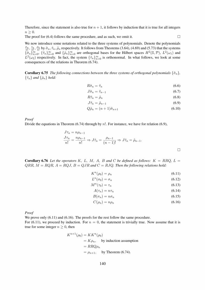
Therefore, since the statement is also true for n+ 1, it follows by induction that it is true for all integersn ≥ 0.The proof for (6.4) follows the same procedure, and as such, we omit it.

We now introduce some notations related to the three systems of polynomials. Denote the polynomialsσnn! ,

τnn! ,

ρnn! by σn, τn, ρn respectively. It follows from Theorems (3.64), (4.69) and (5.73) that the systems

σn∞n=0, τn∞n=0 and ρn∞n=0 are orthogonal bases for the Hilbert spaces H2(S,P), L2(ω1) andL2(ω2) respectively. In fact, the system τn∞n=0 is orthonormal. In what follows, we look at someconsequences of the relations in Theorem (6.74).

Corollary 6.75 The following connections between the three systems of orthogonal polynomials σn,τn and ρn hold:

Rσn = τn (6.6)

Jσn = τn−1 (6.7)

Rτn = ρn (6.8)

Jτn = ρn−1 (6.9)

Qρn = (n+ 1)σn+1 (6.10)

ProofDivide the equations in Theorem (6.74) through by n!. For instance, we have for relation (6.9),

Jτn = nρn−1

Jτnn!

=nρn−1

n!⇒ Jτn =

ρn−1

(n− 1)!⇒ Jτn = ρn−1.

Corollary 6.76 Let the operators K, L, M, A, B and C be defined as follows: K = RRQ, L =QRR, M = RQR, A = RQJ , B = QJR and C = RJQ. Then the following relations hold:

Kn(ρ0) = ρn (6.11)

Ln(σ0) = σn (6.12)

Mn(τ0) = τn (6.13)

A(τn) = nτn (6.14)

B(σn) = nσn (6.15)

C(ρn) = nρn (6.16)

ProofWe prove only (6.11) and (6.16). The proofs for the rest follow the same procedure.For (6.11), we proceed by induction. For n = 0, the statement is trivially true. Now assume that it istrue for some integer n ≥ 0, then

Kn+1(ρ0) = KKn(ρ0)

= Kρn, by induction assumption

= RRQρn

= ρn+1, by Theorem (6.74).

140

Therefore, since the statement is also true for n+ 1, it follows by induction that it is true for all integersn ≥ 0.For (6.16), we use the definition of C and the relations in Theorem (6.74),

C(ρn) = RJQ(ρn)

= RJσn+1

= Rnτn

= nρn.

Corollary 6.77 The following relations hold:

τn(x± i) = ρn(x)± iρn−1(x) (6.17)

σn(x± i) = τn(x)± iτn−1(x) (6.18)

ProofWe prove only (6.17) since the proof for (6.18) follows the same procedure. From corollary (6.75),ρn = Rτn and ρn−1 = Jτn. Thus,

ρn(x)± iρn−1(x) = Rτn(x)± iJτn(x)

= (R± iJ)τn(x)

= τn(x± i), by relation (4.3).

7. Two Bounded OperatorsIn this section, we study two more operators, namely T = R−1 and S = JR−1, where J and R arethe operators that where defined and presented in section (). It is clear from the connections in corollary(6.75) that

T ρn = τn (7.1)

T τn = σn (7.2)

Sτn = τn−1 (7.3)

Sρn = ρn−1 (7.4)

Also by relation (4.3),

Tf(x± i) = (R+ iJ)Tf(x)

= RTf(x) + iJTf(x)

= f(x) + iSf(x). (7.5)

The integral representations of these two operators, S and J , were developed and presented in Araaya’spaper [5]. For the operator T , we have

Tf =1

2 cosh π2x∗ f, (7.6)

141

and for the operator S, we have

Sf = − 1

2 sinh π2x∗ f, (7.7)

where in both cases ∗ denotes convolution. Using the convolution theorem, the Fourier transforms for Tand S were shown to be

T f(t) = sech tf(t) (7.8)

and

Sf(t) = −i tanh tf(t) (7.9)

respectively. We shall also make use of what is known as the Plancherel theorem which states that||f || = ||f || for any f ∈ L2(R). See [13, thm. 9.13].

Proposition 7.78 For the operator T , we have the following:

1. T is linear and bounded from L2(ω2) to L2(ω1).

2. If L20(ω1) = f ∈ L2(ω1) : 〈f, 1〉 = 0 and H2

0 (S,P) = f ∈ H2(S,P) : f(0) = 0, thenT/√

2 is a unitary operator from L20(ω1) onto H2

0 (S,P).

Remark 5 Let f ∈ L2(ω1) and bn = 〈f, τn〉. Then the operator U : L2(ω1) → H2(S,P) defined byUf = b0 + 1√

2

∑∞n=1 bnσn is unitary.

ProofSince all other properties are clear, we prove only boundedness.

1. Let f ∈ L2(ω2) and an = 〈f, ρn〉. By Theorem (5.73), the system ρn∞n=0 is an orthogonalbasis in L2(ω2) with norm

√n+ 1, and so, by proposition (2.56),

f =

∞∑n=0

anρn and ||f ||2L2(ω2) =

∞∑n=0

(n+ 1)|an|2.

By relation (7.1),

Tf =∞∑n=0

anτn.

Since by Theorem (3.64) the system τn∞n=0 is an orthonormal basis in L2(ω1), we have

||Tf ||2L2(w) =∞∑n=0

|an|2

≤∞∑n=0

(n+ 1)|an|2

= ||f ||2L2(ω2),

which proves boundedness of T from L2(ω2) to L2(w) with norm 1.

142

2. Let f ∈ L20(ω1) and bn = 〈f, τn〉. Then b0 = 〈f, τ0〉 = 〈f, 1〉 = 0, and since by Theorem (3.64)

the system τn∞n=0 is an orthonormal basis in L2(ω1), we have

f =

∞∑n=1

bnτn and ||f ||2L20(ω1) =

∞∑n=1

|bn|2.

By relation (7.2),

Tf =∞∑n=1

bnσn.

Since by Theorem (4.69) the system σn∞n=0 is an orthogonal basis in H2(S,P) with norm 1 forn = 0 and

√2 for n ≥ 1, we have

|| 1√2Tf ||2H2

0 (S,P) =∞∑n=1

|bn|2 = ||f ||2L2(ω1).

This proves that T/√

2 is an isometry.

Before proceeding further, we present three lemmas that will be useful in proving the main results of thissection. The proof of the next lemma depends on Cauchy’s theorem [2, thm. 1.4.2] which says that iftwo different paths connect the same two points, and a function is holomorphic everywhere in betweenthe two paths, then the two path integrals of the function will be the same.

Lemma 7.79 If f ∈ H2(S) then f ∈ L2(R, cosh 2t dt) where f is the Fourier transform of an analyticfunction f . Furthermore, ||f ||2H2(S) = ||f ||2L2(R,cosh 2t dt).

ProofRecall from subsection () that analytic functions in the Hilbert space H2(S) have the norm

||f ||H2(S) =

∞∫−∞

|f(x+ i)|2 + |f(x− i)|2

2dx.

For f(x+ i), we have the Fourier transform

1

2π

∞∫−∞

f(x+ i)e−ixtdx =1

2π

∞∫−∞

f(x+ i)e−i(x+i)tetdx

= et1

2π

∞∫−∞

f(x)e−ixtdx, by Cauchy’s theorem

= etf(t).

Similarly for f(x− i),

1

2π

∞∫−∞

f(x− i)e−ixtdx = e−tf(t).

143

It therefore follows by the Plancherel theorem that

||f ||H2(S) =

∞∫−∞

|f(x+ i)|2 + |f(x− i)|2

2dx

=1

2π

∞∫−∞

|etf(t)|2 + |e−tf(t)|2

2dt

=1

2π

∞∫−∞

|f(t)|2(e2t + e−2t

2

)dt

=1

2π

∞∫−∞

|f(t)|2 cosh 2t dt

= ||f ||L2(R,cosh 2t dt).

The proof of the next lemma depends on the Hadamard three-lines theorem [13, thm. 12.8] which for ourparticular case says that if f ∈ A0(S) and if M(n) = max |f(x+ in)| then M(0) ≤ (M(−1)M(1))

12 .

Lemma 7.80 If f ∈ H2(S) then ||f ||0 ≤ (||f ||+1 · ||f ||−1)12 where we have used the notation ||f ||2n =∫∞

−∞ |f(x+ in)|2dx.

ProofDefine the convolution F = f ∗ f ∈ A0(S) where f(x) = f(−x), that is,

F (z) =

∞∫−∞

f(z − x)f(x)dx.

Then

F (0) =

∞∫−∞

|f(−x)|2dx = ||f ||20.

Recall from subsection () that A0(S) is the space of functions that are analytic in S, continuous on ∂Sand f(x+ iy)→ 0 as |x| → ∞. Thus f(x+ in) attains a maximum, say, F (n) = maxx∈R |f(x+ in)|.Then by the Hadamard three-lines theorem [13, thm. 12.8],

F (0) ≤ (F (+1)F (−1))12 ,

and by the Schwarz inequality,

F (+1) ≤ ||f ||+1 · ||f ||0 and F (−1) ≤ ||f ||−1 · ||f ||0.

Therefore,

||f ||20 = F (0) ≤ (F (+1)F (−1))12

≤ (||f ||+1 · ||f ||0 · ||f ||−1 · ||f ||0)12

≤ (||f ||+1 · ||f ||−1)12 ||f ||0

144

so that

||f ||0 ≤ (||f ||+1 · ||f ||−1)12

Lemma 7.81 For all x ≥ 0,√x2 + 1

2 cosh π2x≤ π

2

x

2 sinh π2x

ProofThis is equivalent to proving the inequality

tanhπ

2x ≤ π

2

x√1 + x2

.

For all x ≥ 0, define

f(x) =π

2

x√1 + x2

− tanhπ

2x.

Then,

f(0) = 0 and f ′(x) =π

2

(1

(1 + x2)3/2− sech2 π

2x

).

We need to show that f ′ > 0 for all x > 0. This is equivalent to proving the inequality(1

(1 + x2)3/2− sech2 π

2x

)> 0

cosh2 π

2x > (1 + x2)3/2

cosh4 π

2x > (1 + x2)3 (7.10)

Inequality (7.10) can be proved using Maclaurin series expansion, that is,

(coshπx

2)4 > (1 +

π2x2

8)4 > (1 + x2)4 > (1 + x2)3.

We have thus showed that f ′(x) > 0 for all x > 0, and since f(0) = 0, it follows that for all x ≥ 0,

f(x) ≥ 0π

2

x√1 + x2

− tanhπ

2x ≥ 0

tanhπ

2x ≤ π

2

x√1 + x2

√x2 + 1

2 cosh π2x≤ π

2

x

2 sinh π2x.

We now have all the necessary definitions and lemmas needed to present and prove the main results ofthis section. In fact, they are the final results for this project thesis, and they will be presented in twoseparate theorems, one for the operator T and the other for the operator S.

145

Theorem 7.82 The operator S is linear and bounded on the following Hilbert spaces with norm 1:

1. L2(ω2)

2. L2(ω1)

3. L2(R)

4. H2(S,P)

5. H2(S)

ProofSince linearity follows immediately from the fact that S is a convolution, we shall prove only bounded-ness.

1. Let ˜ρn = ρn√n+1

, f ∈ L2(ω2) and an = 〈f, ˜ρn〉. Since by equation (5.10)√n+ 1 is the norm of

the polynomial ρn in the Hilbert space L2(ω2), it follows from Theorem (5.73) that ˜ρn∞n=0 isan orthonormal basis in L2(ω2). Thus by proposition (2.56),

f =∞∑n=0

an ˜ρn and ||f ||2 =

∞∑n=0

|an|2.

By relation (7.4),

Sf =

∞∑n=1

an

(ρn−1√n+ 1

)

=∞∑n=0

an+1

(ρn√n+ 2

)

=

∞∑n=0

an+1

(√n+ 1

n+ 2

)(ρn√n+ 1

)

=∞∑n=0

(√n+ 1

n+ 2

)an+1

˜ρn.

Thus,

||Sf ||2 =∞∑n=0

(n+ 1

n+ 2

)|an+1|2 =

∞∑n=1

(n

n+ 1

)|an|2 ≤

∞∑n=1

|an|2 ≤ ||f ||2,

which proves boundedness of S on L2(ω2) with norm 1.

2. Let f ∈ L2(ω1) and bn = 〈f, τn〉. By Theorem (3.64), the system τn∞n=0 is an orthonormalbasis in L2(ω1) so that by proposition (2.56),

f =∞∑n=0

bnτn and ||f ||2 =∞∑n=0

|bn|2.

By relation (7.3),

Sf =

∞∑n=1

bnτn−1 =

∞∑n=0

bn+1τn.

146

Thus,

||Sf ||2 =

∞∑n=0

|bn+1|2 =∞∑n=1

|bn|2 ≤∞∑n=0

|bn|2 = ||f ||2,

which boundedness of S on L2(ω1) with norm 1.

3. Let f ∈ L2(R). Using the Plancherel theorem, we have

||Sf ||2 = ||Sf ||2 =1

2π

∞∫−∞

|Sf(t)|2 dt

=1

2π

∞∫−∞

| tanh tf(t)|2 dt, by (7.9)

≤ 1

2π

∞∫−∞

|f(t)|2 dt, since | tanh t| ≤ 1

= ||f ||2

which proves boundedness of S on L2(R) with norm 1.

4. Let ˜σn = 1 if n = 0, and ˜σn = σn√2

for all n ≥ 1. Then by Theorem (4.69), the system ˜σn∞n=0

is an orthonormal basis in H2(S,P). Let f ∈ H2(S,P) and cn = 〈f, ˜σn〉. By proposition (2.56),

f =

∞∑n=0

cn ˜σn and ||f ||2 =

∞∑n=0

|cn|2.

Since RJ = JR by proposition (4.68), it follows that S = JR−1 = R−1J . Thus Sσn = σn−1

by corollary (6.75) so that

Sf =∞∑n=1

cn

(σn−1√

2

)

=

∞∑n=0

cn+1

(σn√

2

)

=c1√

2+∞∑n=1

cn+1˜σn.

Thus,

||Sf ||2 =|c1|2

2+

∞∑n=1

|cn+1|2 =|c1|2

2+

∞∑n=2

|cn|2 ≤∞∑n=1

|cn|2 ≤ ||f ||2,

which proves boundedness of S on H2(S,P) with norm 1.

147

5. Let f ∈ H2(S). Then by Lemma (7.79),

||Sf ||2H2(S) = ||Sf ||2L2(R,cosh 2t dt)

=1

2π

∞∫−∞

|Sf(t)|2 cosh 2t dt

=1

2π

∞∫−∞

| tanh tf(t)|2 cosh 2t dt, by (7.9)

≤ 1

2π

∞∫−∞

|f(t)|2 cosh 2t dt, since | tanh t| ≤ 1

= ||f ||2L2(R,cosh 2t dt)

= ||f ||2H2(S),

which proves boundedness of S on H2(S) with norm 1.

Theorem 7.83 The operator T is linear and bounded on the following Hilbert spaces:

1. L2(ω2) with norm less than or equal to√π.

2. L2(ω1) with norm less than or equal to 2.

3. L2(R) with norm 1.

4. H2(S) with norm 1.

ProofSince linearity follows immediately from the fact that S is a convolution, we shall prove only bounded-ness.

1. We first show that if f ∈ L2R(ω2) and ψ =

√ω2, then Tfψ ∈ H2(S). In particular, we show that

||Tfψ||2H2(S) =

∞∫−∞

|Tf(x+ i)ψ(x+ i)|2 + |Tf(x− i)ψ(x− i)|2

2dx

is finite. Now,

|ψ(x± i)|2 =

∣∣∣∣ x± i2 sinh π

2 (x± i)

∣∣∣∣ =

∣∣∣∣ x± i±i 2 cosh π

2x

∣∣∣∣ =

√x2 + 1

2 cosh π2x, (7.11)

and by relation (7.5),

|Tf(x± i)|2 = |f(x) + iSf(x)|2 = |f(x)|2 + |Sf(x)|2. (7.12)

148

Thus by (7.11) and (7.12),

|Tf(x+ i)ψ(x+ i)|2 = |Tf(x− i)ψ(x− i)|2 (7.13)

=(|f(x)|2 + |Sf(x)|2

) √x2 + 1

2 cosh π2x. (7.14)

Therefore,

||Tfψ||2H2(S) =

∞∫−∞

|Tf(x+ i)ψ(x+ i)|2 + |Tf(x− i)ψ(x− i)|2

2dx

=

∞∫−∞

|Tf(x+ i)ψ(x+ i)|2dx, by (7.13)

=

∞∫−∞

(|f(x)|2 + |Sf(x)|2

) √x2 + 1

2 cosh π2xdx, by (7.14)

≤ π

2

∞∫−∞

(|f(x)|2 + |Sf(x)|2

) x

2 sinh π2xdx, by lemma (7.81)

=π

2

∞∫−∞

|f(x)|2ω2dx+π

2

∞∫−∞

|Sf(x)|2ω2dx

=π

2||f ||2L2

R(ω2) +π

2||Sf ||2L2

R(ω2)

≤ π

2||f ||2L2

R(ω2) +π

2||f ||2L2

R(ω2), by Theorem (7.82) part(1)

= π ||f ||2L2R(ω2), (7.15)

which proves that Tfψ ∈ H2(S) for any f ∈ L2R(ω2).

Next, we show that T is bounded on L2R(ω2). Let f ∈ L2

R(ω2), then

||Tf ||2L2R(ω2) =

∞∫−∞

|Tf(x)|2ω2(x)dx

=

∞∫−∞

|Tf(x)√ω2(x)|2dx

=

∞∫−∞

|Tf(x)ψ(x)|2dx

≤

∞∫−∞

|Tf(x+ i)ψ(x+ i)|2dx

12 ∞∫−∞

|Tf(x− i)ψ(x− i)|2dx

12

=

∞∫−∞

|Tf(x+ i)ψ(x+ i)|2dx, by (7.13)

≤ π ||f ||2L2R(ω2), by (7.15)

149

where the first inequality follows by Lemma (7.80) since Tfψ ∈ H2(S).

We have shown that T is bounded on L2R(ω2) with norm

√π. Now since every analytic function

g can be written as g = f + i h for f, h ∈ L2R(ω2), it follows that T is bounded on L(ω2) with

norm√π.

Remark 6 Since T and S map functions that are real on the real line to functions that also havethis property and therefore T (f + ih) = Tf + iTh, the same bounds hold for complex-valuedfunctions as for real-valued.

2. We first show that if f ∈ L2R(ω1) and ϕ = 1/(2 cosh π

4x), then Tfϕ ∈ H2(S). In particular, weshow that

||Tfϕ||2H2(S) =

∞∫−∞

|Tf(x+ i)ϕ(x+ i)|2 + |Tf(x− i)ϕ(x− i)|2

2dx

is finite. Now, ∣∣∣2 coshπ

4(x± i)

∣∣∣2 =∣∣∣√2 cosh

π

4x± i

√2 sinh

π

4x∣∣∣2

=(√

2 coshπ

4x)2

+(√

2 sinhπ

4x)2

= 2 coshπ

2x,

and so,

|ϕ(x± i)|2 =1

2 cosh π2x. (7.16)

By relation (7.5),

|Tf(x± i)|2 = |f(x) + iSf(x)|2 = |f(x)|2 + |Sf(x)|2. (7.17)

Thus by (7.16) and (7.17),

|Tf(x+ i)ϕ(x+ i)|2 = |Tf(x− i)ϕ(x− i)|2 (7.18)

=(|f(x)|2 + |Sf(x)|2

) 1

2 cosh π2x. (7.19)

150

Therefore,

||Tfϕ||2H2(S) =

∞∫−∞

|Tf(x+ i)ϕ(x+ i)|2 + |Tf(x− i)ϕ(x− i)|2

2dx

=

∞∫−∞

|Tf(x+ i)ϕ(x+ i)|2dx, by (7.18)

=

∞∫−∞

(|f(x)|2 + |Sf(x)|2

) dx

2 cosh π2x, by (7.19)

=

∞∫−∞

|f(x)|2ω1dx+

∞∫−∞

|Sf(x)|2ω1dx

= ||f ||2L2R(ω1) + ||Sf ||2L2

R(ω1)

≤ ||f ||2L2R(ω1) + ||f ||2L2

R(ω1), by Theorem (7.82) part(2)

= 2||f ||2L2R(ω1), (7.20)

which proves that Tfϕ ∈ H2(S) for any f ∈ L2R(ω1).

Next, we show that T is bounded on L2R(ω1). Let f ∈ L2

R(ω1), then

∞∫−∞

|Tf(x)ψ(x)|2dx =

∞∫−∞

|Tf(x)|2(2 cosh π

4x)2dx

=

∞∫−∞

|Tf(x)|2

2(cosh π

2x+ 1)dx

≥∞∫−∞

|Tf(x)|2

2(cosh π

2x+ cosh π2x)dx, since cosh

π

2x ≥ 1

=

∞∫−∞

|Tf(x)|2

4 cosh π2xdx

=1

2

∞∫−∞

|Tf(x)|2ω1(x)dx

151

so that

||Tf ||2L2R(ω1) =

∞∫−∞

|Tf(x)|2ω1(x)dx

≤ 2

∞∫−∞

|Tf(x)ϕ(x)|2dx

≤ 2

∞∫−∞

|Tf(x+ i)ϕ(x+ i)|2dx

12 ∞∫−∞

|Tf(x− i)ϕ(x− i)|2dx

12

= 2

∞∫−∞

|Tf(x+ i)ϕ(x+ i)|2dx, by (7.18)

≤ 4||f ||2L2R(ω1), by (7.20)

where the second inequality follows by the Lemma (7.80) since Tfϕ ∈ H2(S).

We have shown that T is bounded on L2R(ω1) with norm 2. Now since every analytic function g

can be written as g = f + i h for f, h ∈ L2R(ω1), it follows by Remark (6) that T is bounded on

L(ω1) with norm 2.

3. Let f ∈ L2(R). Using the Plancherel theorem, we have

||Tf ||2 = ||T f ||2 =1

2π

∞∫−∞

|T f(t)|2 dt

=1

2π

∞∫−∞

| sech tf(t)|2 dt, by (7.8)

≤ 1

2π

∞∫−∞

|f(t)|2 dt, since | sech t| ≤ 1

= ||f ||2

which proves boundedness of T on L2(R) with norm 1.

152

4. Let f ∈ H2(S). Then by Lemma (7.79),

||Tf ||2H2(S) = ||T f ||2L2(R,cosh 2t dt)

=1

2π

∞∫−∞

|T f(t)|2 cosh 2t dt

=1

2π

∞∫−∞

| sech tf(t)|2 cosh 2t dt, by (7.8)

≤ 1

2π

∞∫−∞

|f(t)|2 cosh 2t dt, since | sech t| ≤ 1

= ||f ||2L2(R,cosh 2t dt)

= ||f ||2H2(S),

which proves boundedness of T on H2(S) with norm 1.

References[1] M. Abramowitz and I. A. Stegun. Handbook of Mathematical Functions. Dover Publications, Inc.,

New York, 1965.

[2] L. V. Ahlfors. Complex Analysis: An Introduction to the Theory of Analytic Functions of OneComplex Variable. 3rd ed., Mc-Graw-Hill, 1979.

[3] G. E. Andrews, R. Askey and R. Roy. Special Functions. Cambrige University Press, Cambrige,2000.

[4] T. K. Araaya. The Meixner-Pollaczek Polynomials and a System of Orthogonal Polynomials in aStrip. Uppsala, 1999.

[5] T. K. Araaya. Umbral Calculus and the Meixner-Pollaczek Polynomials. Uppsala, 2002.

[6] K. N. Chaudhury. Lp-Boundedness of the Hilbert Transform. arXiv:0909.1426v8 [cs.IT], 2010.

[7] L. Holst. Probabilistically Proving Some Identities of Euler. Department of Mathematics, KTH,SE-10044 Stockholm, Sweden.

[8] E. Koelink. Spectral Theory and Special Functions. arXiv:math/0107036v1 [math.CA], 2001.

[9] T. W. Korner. A Companion to Analysis: A Second First and First Second Course in Analysis.American Mathematical Society, 2004.

[10] E. Laeng. A Simple Real-Variable Proof that the Hilbert Transform is an L2-Isometry. C. R. Acad.Sci. Paris, Ser. I 348 (2010) 977980.

[11] M. Reed and B. Simon. Methods of Modern Mathematical Physics. Vol. 1 Functional Analysis.Academic Press Inc., New York, 1980.

153

[12] W. Rudin. Principles of Mathematical Analysis. Third edition, McGraw-Hill International Editions,1976.

[13] W. Rudin. Real and Complex Analysis. International Student Edition, McGraw-Hill, New York,1970.

[14] J. Shen. Orthogonal Polynomials and Polynomial Approximations: Chapter 3. Department ofMathematics, Purdue University, 2009.

[15] G. F. Simmons and S. G. Krantz. Differential Equations: Theory, Technique, and Practice.McGraw-Hill International Edition, New York, 2007.

[16] E. M. Stein and G. Weiss. Introduction to Fourier Analysis on Euclidean Spaces. Princeton Uni-versity Press, 1971, pp. 205-209.

[17] G. Szego. Orthogonal Polynomials. Amer. Math. Soc. Colloq. Pubb. 23, Fourth Edition, 1975, pp395.

[18] V. Totik. Orthogonal Polynomials. Surveys in Approximation Theory, Volume 1, 2005. pp. 70125.

154

ABSTRACTS

Asymptotic Properties of The Delannoy Numbers and Similar Arraysby

Christer [email protected]

Uppsala University, Department of Mathematics, Uppsala, Sweden

Abstract: Abstract: The Delannoy numbers were introduced and studied by Henri-Auguste Delannoy(1833-1915). He investigated the possible moves on a chessboard: the numbers under considerationappear when one studies “la marche de la Reine,” i.e., how the queen moves (the binomial coefficientsappear similarly for the moves of the rook). The asymptotic behavior of the array of Delannoy numbersis studied. The regularized upper and lower radial indicators of the array are determined, proved tocoincide, and to be concave. We also describe the radial indicator as an infimum of linear functions,which amounts to determining its Fenchel transform. Since the methods developed for this study applyto more general convolution equations, we prove results also for these equations.

The (Dis)connectedness of Products in the Box Topologyby

Vitalij A. ChatyrkoDepartment of Mathematics, Linkoping University, Linkoping, Sweden

Abstract: In this talk we suggest two independent sufficient conditions on topological connected spaceswhich imply disconnectedness, and one sufficient condition which implies connectedness, of productsof spaces endowed with the box topology. Some applications of that will be also presented.

Identification of Coefficients in Parabolic Equations Using Measurements on the Boundaryby

Frerik BerntssonLinkping University, Sweden

Abstract: To determine the thermal conductivity in the interior of a body using measurements onthe boundary is an important problem. Applications arise, e.g., in methods for non-destructive testingof adhesive bonds, or crack detection in metallic materials. In our application we measure the time-dependent temperature and heat-flux at certain locations on the boundary, or inside the domain, andattempt to reconstruct the thermal conductivity as accurately as possible. The coefficient identificationproblem is severely ill-posed in the sense that small changes in the measured data can lead to largechanges in the computed solution. The ill-posedness is analyzed using the singular value decomposition.Also, the recorded data may not contain any information about the unknown coefficient. We propose toformulate the coefficient identification problem as a non-linear least squares problem. The problem canbe solved using the Gauss-Newton method. The dimension of the least squares problem is reduced by

155

modelling the unknown coefficient using only a small number of parameters. Numerical tests show thatthe method works well.

Multidisciplinary Research in Mathematical Sciences With Applications to Real World Problemsin Biological, Bio-Inspired and Engineering Systems

byPadmanabhan Seshaiyer

George Mason University, USA Email: [email protected]

Abstract: Computational mathematics, which comprises of mathematical modeling, analysis and sim-ulation, is quickly becoming the foundation for solving most complex applications in biological, bio-inspired and engineering systems. Breakthrough research required to solve such complex problemsinvolves transformative and multidisciplinary efforts spanning scientific and engineering disciplines.In this talk, we will describe research methods using mathematical modeling, analysis and computa-tional techniques to explain fundamental mechanisms needed to understand the quantitative behaviorunderlying real-world applications. Specific examples of interdisciplinary projects involving analyticaland numerical solutions to partial differential equations that can help to encourage students to learn bydiscovery to enhance their understanding of the multidisciplinary role of mathematics in engineering,science and medicine will be presented.

Epidemic Potential for Malaria in Epidemiological Zones in Kenyaby

Wandera OganaSchool of Mathematics, University of Nairobi, Kenya

Abstract: Malaria is a vector-borne disease which annually results in over one million deaths andfive hundred million clinical episodes, most of which occur in sub-Sahara Africa. Since the diseaseis influenced by climate factors, it is important to assess the possible risk posed by climate change onmalaria transmission. A number of indices can be used to assess this risk but the most appropriateappears to be the epidemic potential, which is derived from the basic reproduction number, R0. Wedetermine the epidemic potential for selected areas within the four epidemiological zones in Kenya,using modeled temperature and rainfall data. For the years 2009 to 2011, for which detailed malariadata is available, we compare the variation in epidemic potential with malaria incidence. Results showthat the variation in epidemic potential, from month to month, reflects a pattern similar to the variationin malaria incidence.

How to Manipulate Derangementsby

Fanja Rakotondrajao,University of Antananarivo, Madagascar

Abstract: We are living in a period of change or/and of conflict: for example, the climate change,the trend to electronic systems, and so on. All these changes will also change our way of life. In

156

combinatorial word, we say that there are derangements. But ”derangements are like a rose bush, whenyou touch them; you need to be careful of thorns.” We will give different methods how to manipulatederangements combinatorially and how to analyze them.

The Dynamics of Populations in Wetlandsby

Abdou SeneGaston Berger University

Abstract: Some wetlands are centers of important migrations of populations of various species. Theseinterdependent migrations, caused by economic and environmental factors, are governed by Mathemati-cal nonlinear complexe systems. This work consists in developing and analysing a Mathematical modelof interconnection among:

• The quantity and quality of the water available in the wetland

• The size of the population of fish in the waterways

• The dynamics of migrating birds population

• The size of the tourists population

• The dynamics of human populations going to or coming from the sorrounding towns or villages.

Adaptive Markov Chain Monte Carlo Using Variational Bayesian Adaptive Kalman Filterby

Isambi Sailon Mbalawata and Simo SarkkaLappeenranta, Finland

Abstract: When we analyze the high dimensional complex models, the computation of the normal-ized posterior density and its expectations are intractable hence we employ the numerical approximationtechniques such as Markov chain Monte Carlo methods. Markov chain Monte Carlo (MCMC) methodis a powerful computational tool for analysis of complex statistical problems; it requires proper tuningof proposal distribution for better mixing of chains and suitable acceptance rate. However, in practicethe selection of a proper proposal distribution is not a trivial task because manual tuning of proposaldistribution is time consuming and laborious. The most used proposal distribution is the Gaussian distri-bution, due to its attractive computational and theoretical properties. One problem of Gaussian proposaldistribution is how to find a suitable covariance matrix. One way to overcome this problem is to use theadaptive Markov chain Monte Carlo algorithm. The algorithm automatically tunes the covariance matrixduring MCMC run. In this work, we propose a new adaptive MCMC algorithm where the covariancematrix is adapted using variational Bayesian adaptive Kalman filter. Numerical results for simulatedexamples are presented and discussed in detail.

157

Linear Estimation of Location and Scale Parameters for Logistic Distribution Based onConsecutive Order Statistics

byPatrick G. O. Weke

School of Mathematics University of Nairobi, Kenya

Abstract: Linear estimation of the scale parameter of the logistic population based on the sum ofconsecutive order statistics when the location parameter is unknown is discussed. A method based on apair of single spacing and the ’zero-one’ weights rather than the optimum weights is presented and usedto compute the bias, variance and relative efficiencies with respect to variance Cramer-Rao lower boundand best linear unbiased estimators (BLUE’s) for sample size . Finally, a comparison of these estimatorsis discussed.

A Stochastic Model for Planning a Compartmental Education System and Supply of Manpowerby

Lydia MusigaUniversity of Nairobi, Nairobi, Kenya

Abstract: This paper describes a Markov Chain transition model that encompasses the different com-partments of an education system. The model clearly shows transition rates within compartments andalso between compartments, thus planners in the country will understand better the flow of studentsfrom primary school to university level. Also, the theory of Absorbing Markov Chains, specifically theChapman-Kolmogorov result, assists in predicting future enrolments. Hence, the model will facilitatemore effective planning in the country’s education system and in the supply of manpower.

Financial Sector Performance Enhancersby

Emma Anyika and Patrick WekeUniversity of Nairobi, Nairobi, Kenya

Abstract: In any state or country there are certain sectors that are relied upon to drive its economy.For many of these countries the financial sector is seen as the driving force of the economy. This iswitnessed in many World economic crises which commence with the large organisations in the financialsector. This should aid entrepreneurs to be aware of the areas of emphasis and factors for considerationfor positive growth of their organisations. Existing organisations will also benefit by improving the saidareas and adopting the factors for continued growth and sustainability. A multiple regression modelwill be used to relate performance to its causes. Tests of hypothesis will then be made to allow for thegeneralization of the findings to the whole population

158

Estimating the List Size Using Bipartite Graph for Colouring Problemsby

Mashaka MkandawileUniversity of Dar es Salaam

Abstract: In graph theory a bipartite graph is a graph whose vertices can be divided into two disjointsets U and V such that every edge connects a vertex in U to one in V ; that is, U and V are independentsets. Bipartite graphs show up in many places and are therefore often used tool to model and calculatewith. Let B(n,m) be a bipartite graph with n vertices in each side and m edges. For each vertex wedraw uniformly at random a list of size k from a base set N of size n. In this paper we estimate the sizesof n and k so that B(n,m) has a perfect matching with high probability.

Mathematical Modeling of Pneumonia Transmission Dynamicsby

Emaline Joseph, Kgosimore and Teresia Marijani.

Department of Mathematics, University of Dar-es-Salaam Tanzania . Abstract: Pneumonia is oneof the leading causes of serious illness and deaths among children and adults around the world. Wetherefore, formulate and analyze a mathematical model of the transmission dynamics of pneumoniawith the aim of understanding its transmission dynamics. The study also evaluates the impact of controland prevention strategies in curtailing or mitigating against the spread of disease. We derive conditionsfor the clearance or persistence of the pneumonia infection through the stability of the equilibria. Weinfer the impact of control strategies on the dynamics of the disease through sensitivity analysis of thereproduction number, R0. Numerical simulations are carried out to illustrate the analytical results andtest the influence of certain parameters. The result of study showed that treatment and vaccination havethe effect of reducing the disease provided that the control reproduction number is reduced to a valuebelow one

Hydrodynamics of Shallow Water Equations: A Case Study of Lake Victoriaby

David Ddumba WalakiraMathematics Department, Makerere University

Abstract: A three dimensional hydrodynamic model has been applied to lake Victoria. We have as-sumed a vertical coriolis dominance because of the geographical location of lake Victoria at the equator,leading to a non-hydrostatic approximation. To capture not only the dis-continuities, but also the physi-cal and numerical shocks in the shallow water flow of the second largest fresh water body in the world,a min-mod flux limiter has been employed as a numerical finite volume high resolution method to solvea 3D model with Boussines and swallow water approximations. An energy method is applied for thewell-posedeness of this non-linear hyperbolic system of equations.

159

Boundary Layer Flow Over a Moving at Surface With Temperature Dependent Viscosityby

J.W. MwaonanjiMathematics and Statistics Dept, The Polytechnic, University of Malawi, Malawi

Abstract: Numerical investigation of two-dimensional laminar boundary layer flow over a movingflat surface with temperature dependent viscosity is studied. The flow is divided into two regimes: withviscous dissipation and without viscous dissipation. The flow is also restricted to a region where both thefree-stream and the flat surface are moving in the same direction i.e no reverse flow within the boundarylayer. Thus the velocity ratio, ξ, has generally been chosen in such a way that 0 < ξ < 1. The governingboundary layer equations of the flow are transformed to a dimensionless system of equations using asimilarity variable ζ(x, y). The resulting set of coupled non-linear ordinary differential equations aresolved numerically by applying shooting iteration technique together with fourth-order Runge-Kuttaintegration scheme. The effects of the various parameters of the flow e.g velocity variation variable, ξ,viscosity variation parameter, ε, etc. on velocity and temperature distribution in the boundary layer, onthe local skin friction and local heat transfer coefficients are investigated.

Absolute-Convective Instability of Mixed Forced-Free Convection Boundary Layersby

Eunice MureithiMathematics Department, University of Dar es salaam

Abstract: A spatio-temporal inviscid instability of a mixed forced-free convection boundary layeris investigated. The base flow considered is the self-similar flow with free-stream velocity µ ∼ xn.Such a boundary layer flow presents the unusual behaviour of generating a region of velocity overshoot,in which the stream-wise velocity within the boundary layer exceeds the free-stream speed. A linearstability analysis has been carried out. Saddle points have been located and a critical value for thebuoyancy parameter, G0 = G0C ≈ 3.6896, has been determined below which the flow is convectivelyunstable and above which the flow becomes absolutely unstable. Two families of spatial modes havebeen obtained, one family being of convective nature and the other of absolute nature. The convectivetype spatial mode shows mode crossing behaviour at lower frequencies. Thermal buoyancy has beenshown to be destabilizing to absolutely unstable spatial mode.

Optimal Premium Policy of an Insurance Firm With Delayby

Moses MwaleUniversity of Dar es Salaam, Tanzania

Abstract: In this work, we study the optimization problem confronted by an insurance firm whosemanagement can control its cash-balance dynamics by adjusting the underlying premium rate. The firm’sobjective is to minimize the total deviation of its cash-balance process to some pre-set target levels byselecting an appropriate premium policy. We make two inclusions to the problem; Firstly, we introducethe aspect of time delay to the system. Delay systems may occur in several situations, e.g. in financeand biology where the growth of the state depends not only on the current value of the state but also

160

on previous state values. Stochastic delay differential equations (SDDE’s) model systems with delay.The second inclusion is that we replace the standard expected additive utility function with a Stochasticdifferential utility (SDU). A SDU is an extension of the notion of recursive utility to a continuous-time, stochastic setting. It allows us to disentangle risk aversion and inter temporal substitution. Thepaper is devoted to the study of optimal control of stochastic differential delay equations in a firstly ingeneral framework. The Martingale Representation Theorem is applied to obtain a Backward StochasticDifferential Equation (BSDE) which represents the utility function. The resulting system is a Forward-Backward Stochastic Differential Equation which is not fully coupled and we also assume that it isquadratic in the cash-balance and control variables. We establish existence and prove for uniqueness ofthe solution to our FBSDE. We then also establish sufficient and necessary maximum principles for anoptimal control of such systems. We end with a case study of two particular works which fit into ourgeneral model.

On the Coexistence of Distributional and Rational Solutions for Ordinary Differential EquationsWith Polynomial Coefficients

byG.I. Mirumbe, Vincent SSembatya, Rikard Bgvad and Jan Erik Bjork

Abstract: Given an ordinary differential equation with polynomial coefficients, Wiener & Cooke (1990)gave a necessary and sufficient condition for the simultaneous existence of solutions to ordinary dif-ferential equations with polynomial coefficients in the form of finite order linear combination of theDirac-delta function and its derivatives and the rational function solutions using the Laplace transformand functional differential equations techniques. In this paper, we prove a similar result using the the-ory of boundary values and the Cauchy transform. This method has an advantage as it gives a closedform expression for the polynomial q(t) in case the finite order distributional solution and the rationalfunction solution do not satisfy the same differential equation but in different variables

On Modelling and Pricing Index Linked Catastrophe Derivativesby

Philip NgareSchool of Mathematics, University of Nairobi, Kenya

.

Abstract: We consider the problem of indifference pricing of derivatives written on CAT bonds. Theindustrial loss index is modeled by a compound Poisson process and the number of claims as doublystochastic process, such that its intensity varies over time. The insurer can adjust her portfolio by choos-ing the risk loading, which in turn determines the demand. We probably restrict the policies of theinsurance company in a way that does not permit changing the risk loading during catastrophe times.We compute the price of a CAT option written on that index using utility indifference pricing.

161

Optimal Portfolio Management When Stocks are Driven by Mean Reverting Processesby

Lusungu Mbiliri, Charles Mahera, and Sure Mataramvura

Abstract: In this paper we present and solve the problem of portfolio optimization within the context ofcontinuous-time stochastic model of financial variables. We consider an investment problem where aninvestor has two assets, namely, risk-free assets (eg bonds) and risky assets (eg stocks) to invest on andtries to maximize the expected utility of the wealth at some future time . The evolution of the risk-freeasset is described deterministically while the dynamics of the risky asset is described by the geometricmean reversion (GMR) model. The controlled wealth stochastic differential equations (SDE) as well asthe portfolio problem are formulated. Therefore the portfolio optimization problem is then successfullyformulated and solved with the help of the theory of stochastic control technique where the Dynamicprogramming principle (DPP) and the HJB theory are the perfect tools. We obtain the very interestingresults including the solution of the HJB equation which is the non-linear second order partial differentialequation and the optimal policy which is the optimal control strategy of the investment process. So wehave considered utility functions which are members of HARA, called power and exponential utility. Inboth cases, the optimal control (investment strategy) has explicit forms and is wealth dependant, in thesense that, as the investor becomes richer, the less he invests on the risky assets.

On Hub Number of Hypercube and Grid Graphsby

Egbert MujuniMathematics Department, University of Dar es Salaam, Tanzania

Abstract: A set H ⊂ V is a hub set of a graph G = (V,E) if, for every pair of vertices u, v ∈ V −H ,there exists a path from u to v such that all intermediate vertices are in H . The hub number of G isthe minimum size of a hub set in G. In this talk we derive the hub numbers of hypercube and gridgraphs. Meanwhile, new results on the size of maximum leaf spanning tree of grid graph problem arealso obtained.

Fixed Points of Homeomorphisms of Knaster Continuaby

Vincent A SsembatyaMakerere University, Uganda

Abstract: J. Aarts and R. Fokkink proved that every homeomorphism of the standard (dyadic) Knastercontinuum has two fixed points. This answered in the affirmative a question asked by W. Mahavier. Inthis paper we show that for generalized Knaster continua defined by an arbitrary sequence of primes,this result may be false. On the other hand, there are many circumstances where homeomorphisms ongeneralized Knaster continua do have more than one fixed point. In certain cases, one can give a lowerbound to the number of fixed points of a homeomorphism. Very often this lower bound is in fact verylarge. We also discuss a generalization of Knaster continua defined for dimensions greater than one. Weshow that some of the properties of Knaster continua hold for these generalized examples

162

Continuity of Inversion in the Algebra of Locality - Measurable Operatorsby

Isaac Daniel TemboUniversity of Zambia, Zambia

Abstract: Let M be a semi-finite von Neumann algebra in a Hilbert space H and τ be a faithfulnormal semi-finite trace on M . Let Mp denote the lattice of self-adjoint projections in M , I denote theidentity of M , and ||.|| denote the C∗-norm on M . The set of all measurable operators M with sumand product defined as the respective closures of the algebraic sum and product is ∗-algebra. Equippedwith a metrisable vector topology called the topology of convergence in measure τm, M is a completemetrisable topological ∗-algebra in which M is dense. For M , it has been shown that [1]

Proposition LetQ be the set of invertible elements in M , and (Sn) a sequence inQ such that Sn →τm I .Then S−1

n →τm I , that is to say inversion is τm-continuous on Q.

In this talk we present a similar result but for the topology of local convergence in measure, whosedefinition we shall present.

Uniquely Hamiltonian Graphsby

Herbert FleischnerVienna Technical University, Austria

Abstract: To decide whether a graphG has a hamiltonian cycle is an NP-complete problem. However, ifG has no vertices of even degree, then by a theorem of Thomason, every edge belongs to an even numberof hamiltonian cycle. In fact, J.Sheehan asked whether there exists a 4-regular uniquely hamiltoniangraph (i.e., with precisely one hamiltonian cycle), and J.A. Bondy posed the more general questionwhether there is a uniquely hamiltonian graph of minimum degree 3. In this talk we show how one canconstruct uniquely hamiltonian graphs of minimum degree 4 and arbitrary large maximum degree.

The Role of Backward Mutations on the Within Host Dynamics Of HIV-1by

Kitayimbwa M. John, Joseph Y. T. Mugisha and Robert A. Saenz

Abstract: The quality of life for patients infected with human immunodeficiency virus (HIV-1) hasbeen positively impacted by the use of antiretroviral therapy (ART). However, the benefits of ART areusually halted by the emergence of drug resistance. Drug-resistant strains arise from virusmutations,as HIV-1 reverse transcription is prone to errors, with mutations normally carrying fitness costs to thevirus. When ART is interrupted, the wild-type drug-sensitive strain rapidly out-competes the resistantstrain, as the former strain is fitter than the latter in the absence of ART. One mechanism for sustainingthe sensitive strain during ART is given by the virus mutating from resistant to sensitive strains, whichis referred to as backward mutation. This is important during periods of treatment interruptions asprior existence of the sensitive strain would lead to replacement of the resistant strain. In order toassess the role of backward mutations in the dynamics of HIV-1 within an infected host, we analyzea mathematical model of two interacting virus strains in either absence or presence of ART. We study

163

the effect of backward mutations on the definition of the basic reproductive number, and the valueand stability of equilibrium points. The analysis of the model shows that, thanks to both forward andbackward mutations, sensitive and resistant strains co-exist. In addition, conditions for the dominanceof a viral strain with or without ART are provided. For this model, backward mutations are shown to benecessary for the persistence of the sensitive strain during ART.

Comparative Study of the Distributions Used To Model Dispersionby

Kipchirchir, I. C.School of Mathematics, University of Nairobi, Nairobi Kenya

Abstract: The negative binomial distribution has been widely used and to a lesser extent the Ney-man Type A distribution, whereas the Polya-Aeppli distribution has received no attention in modelingoverdispersed (clustered) populations. On the other hand, the Poisson distribution is naturally used tomodel random populations. The aim of this paper is to carry out a comparative study of the aforemen-tioned distributions based on index of patchiness, correlation, skewness and kurtosis. The study revealedthat the negative binomial, the Neyman Type A and the Polya-Aeppli distributions are equivalent in de-scribing dispersion and they have Poisson as a limiting distribution. However, the distributions differin terms of skewness and kurtosis, though the Polya-Aeppli is closer to the negative binomial than theNeyman Type A. Thus, in order to discriminate probability models for over dispersion, an index whichincorporates skewness and kurtosis need to be devised.

A Within Host Model of Blood Stage Malariaby

Theresia MarijaniUniversity of Dar es Salaam, Tanzania

Abstract: Malaria is a deadly tropical disease caused by protozoa of the genus plasmodium. Themalaria parasite life cycle involves three cycles namely the sporogony (mosquito stages), exoerythrocyticschizogony (human liver stages), and the erythrocytic schizogony (human blood stage). We consider amathematical model for malaria involving, susceptible red blood cells, latent infected red blood cells,active infected red blood cells, intracellular parasites, extracellular parasites and effector cells. Themodels is analysed mathematically and numerically. One of the question addressed in our study is: whatreplicative characteristics offer the parasite opportunities to evade the host immune system? The resultsshowed that the longer it takes to produce the parasites, the higher the chance that an infected red bloodcell will be identified and apoptosised by the effector cells. Our sensitivity analysis results show thatpoor parametric estimation has serious implications on the prognosis of the disease. Treatment resultssuggest that a high drug efficacy can stop the development of the disease. The study has revealed thatthe parasite replicative characteristics enable the parasite to evade the immune response during the redblood stage malaria. We have found that the parasite has a strategy of infecting older red blood cellsas a strategy to evade immune surveillance. We recommend treatment to be used in areas where anti-malarial drugs do not show resistance to the parasites. We also recommend that individuals with malariaor showing some symptoms should be treated for both malaria and chronic infections.

164

Application of Stochastic Differential Equations to Model Dispersion of Pollutants in ShallowWater

byWilson Mahera Charles

University of Dar-es-salaam, Tanzania

Abstract: A two dimensional stochastic differential equations(SDEs) to describe the dispersion of pol-lutants in shallow water is developed. By deriving the Kolmogorov’s forward partial differential equa-tion or commonly called Fokker-Planck equation, the SDEs model is shown to be consistent with thetwo-dimensional advection-diffusion equation. To improve the behaviour of the model shortly after thedeployment of the pollutant, the SDEs called random flight model is developed too. It is shown that overlong simulation periods, this model is again consistent with the advection diffusion equation. The simu-lated results in an ideal two dimensional domain are presented to predict the dispersion of a pollutant inthe shallow waters.

Stochastic Model for In-Host HIV Virus Dynamics With Therapeutic Interventionby

R. W. Mbogo, L. LuboobiJ. W. Odhiambo

Abstract: Mathematical models are used to provide insights into the mechanisms and dynamics ofthe progression of viral infection in vivo. Untangling the dynamics between HIV and CD4+ cellularpopulations and molecular interactions can be used to investigate the effective points of interventionsin the HIV life cycle. With that in mind, we develop and analyze a stochastic model for In-Host HIVdynamics that includes combined therapeutic treatment and intracellular delay between the infectionof a cell and the emission of viral particles, which describes HIV infection of CD4+ T-cells duringtherapy. The unique feature is that both therapy and the intracellular delay are incorporated into themodel. Models of HIV infection that include intracellular delays are more accurate representations ofthe biological data. We show the usefulness of our stochastic approach towards modeling combinedHIV treatment by obtaining probability distribution, variance and co-variance structures of the healthyCD4+ cell, and the virus particles at any time t. Our analysis show that, when it is assumed that the drugis not completely effective, as is the case of HIV in vivo, the predicted rate of decline in plasma HIVvirus concentration depends on three factors: the death rate of the virons, the efficacy of therapy and thelength of the intracellular delay.

An Alternating Iterative Procedure for the Cauchy Problem for the Helmholtz Equationby

F. Berntsson, V. Kozlov, L. Mpinganzima, and B.O. TuressonDepartment of Mathematics, Linkoping University, Sweden

Abstract: Let ω be a bounded domain in R2with a Lipschitz boundary Γ divided into two parts Γ0

and Γ1 which do not intersect one another and have a common Lipschitz boundary. We consider thefollowing Cauchy problem for the Helmholtz equation

M u+ k2u = 0 in ωU = f on Γ0

∂vu = g on Γ1

165

where k is the wave number, ∂v denotes the outward normal derivative, and f and g are specified Cauchydata on Γ0. This problem is ill-posed.

The alternating iterative algorithms for solving this problem are developed and studied. These algorithmsare based on the alternating iterative schemes suggested in [1] and [2]. Since these original alternatingiterative algorithms diverge for a large constant k2in the Helmholtz equation, we develop a modificationof the alternating iterative algorithms which converge for such k2. We also perform numerical tests. Thenumerical experiments confirm that the proposed modification works.

166

IndexAbdou Sene, 157Alphonce, 87Anyika, 158

Berntsson, 155, 165Bjork, 161Bgvad, 161

Chatyrko, 155Ciriza, 108

El Tom, 11Evarest, iv

Fleischner, 163

Gahirima, v

Joseph, 159

Kasozi, vKgosimore, 159Kikonko, 52Kipchirchir, 164Kiselman, 155Kitayimbwa John, 163Kozlov, 165Kumar, 72

Luboobi, 81, 165

Mahara, vMahera, 162, 165Makame Mnyaa Mbarawa, 9Makinde, 43Mango, v, 3Marijani, iv, 159, 164Massawe, 1Mataramvura, 162Mbalawata, 157Mbiliri, 162Mbogo, 165Mirumbe, 161Mkandawile, 159Montaz Ali, 61Mpinganzima, 165Mugisha, 163Mujuni, iv, 162Mureithi, iv, 160

Musiga, 158Musonda, 120Mwale, 160Mwaonanji, 160

Ngare, 161

Odhiambo, 165Ogana, 156

Rakotondrajao, 156Rugeihyamu, iv

Saenz, 163Sarkka, 157Seshaiyer, 156Sima, 61Soud, 98Ssembatya, 161, 162

Tembo, vTembo , 163Turesson, 165

Vaderline, 23

Walakira, 159Weke, v, 26, 158

167

COVER PAGE - International Science Programme · 1 Herbert Fleischner Austria 41 Mohamed Eltom Sudan...

Documents

Transcript of COVER PAGE - International Science Programme · 1 Herbert Fleischner Austria 41 Mohamed Eltom Sudan...