cover - ENGINEERING LABORATORY AND...

UNIVERSITI MALAYSIA SARAWAK

FACULTY OF ENGINEERING DEPARMENT OF MECHANICAL AND

MANUFACTURING ENGINEERING

KNJ1241 MECHANICAL AND

MANUFACTURINGENGINEERING

LABORATORY2

LABORATORY MANUAL

TABLE OF CONTENT

Lab Code Title Page

SD1

SD2

SD3

SD4

SD5

SD6

SD7

SD8

SD9

SD10

Deflection of a Beam

Reaction of Continuous Beam

Reaction of Moment for a Fixed End Beam

Reaction of Propped Cantilever Beam

Torsion of Shaft

Flexure Stress

Relation between Angular Speed and Linear Speed

Compound Pendulum

Flywheel Apparatus

Belt Friction

1

5

9

13

17

21

25

29

35

39

Appendix

A

B

Safety First

Guidelines for Laboratory Report

43

44

KNJ1241 Engineering Laboratory 2 Faculty of Engineering Universiti Malaysia Sarawak

1

TITLE :

SD1 – Deflection of a Beam

THEORY :

Deflection of a beam can be described by the degree of the displaced beam or the

displacement of the certain point on the beam under a load application. The deflection of

a beam depends on its length, its cross-sectional shape, the material, where the deflecting

force is applied, and how the beam is supported. The equations given here are for

homogenous, linearly elastic materials, and where the rotations of a beam are small.

Figure 1: Simply Supported Beam

The mid-span deflection of a simply supported beam loaded with a load W at mid-span is

given by;

δ = (1)

Rewriting,

E = Or,

E =

OBJECTIVE :

To establish the relationship between deflection and applied load and determine the

Young Modulus of the beam specimen from the deflection data.

WL3 48 EI

L

L/2

W

L3 48 I

× Slope of the load deflection curve

L3 W 48 I δ


2

APPARATUS :

A support frame, a pair of pinned support, a load hanger, dial gauge, beam specimen, set

of weights.

SAFETY PRECAUTIONS :

Beware of the loose heavy items such as weights and make sure apparatus is well

tightened.

PROCEDURE :

1. Measure width and depth of specimen and record the readings (take measurement at 3

locations and record the average reading)

2. Place the beam specimen between the clamping plates and fix the load hanger at the

mid-span of the beam.

3. Position the dial gauge at the mid-span of the beam to measure the resulting

deflection and set the dial gauge reading to zero. (1 div = 0.01 mm)

4. Place a suitable load on the load hanger then record the resulting dial gauge reading.

Increase the load on the load hanger and record all the result in the table 1.


3

RESULTS :

1. Complete the required data

Span of tested beam, L = mm

Width of beam specimen, b = mm

Depth of beam specimen, d = mm

Moment of inertia of beam specimen, (bd3/12) = mm4

2. Tabulate the table below.

Table 1 : Deflection againts Applied Load

Applied Load

Experimental Deflection Theoretical Deflection

mm

Test 1 Test 2 Average Deflection

mm N div mm div mm

3. Using the tabulated data in the Table 1, plot the graph of load versus experimental

deflection. Draw the best fit curve through the plotted point and hence deduce the

relationship between the applied load and the resulting mid span deflection.

4. Calculate the Modulus of Elasticity using the slope of the graph obtained assuming a

linear relationship between load and deflection as shown below.

DISCUSSION :

1. Discuss the relationship between the load and the experimental deflection and

compare with the theoretical calculation.

2. What does the slope of the graph represents and how does it varies in relation to the

load position.

3. Calculate the Young Modulus from the result obtained and compared the result with

the reference.

4. Discuss the accuracy of the data.


4


5

TITLE :

SD2 – Reaction of a Continuous Beam

THEORY :

Continuous beam is a beam which extends over three or more supports that joined

together. Therefore, the given load on one span will effect on the other spans. Hence the

reaction on the other support can be calculated based on the given load. Typical reactions

at the support of a continuous beam is as shown below

Figure 2: Reaction of Continuous Beam a

Figure 3: Reaction of Continuous Beam b

Figure 4: Reaction of Continuous Beam c

Different arrangement of span and load will give a different value of reaction at the

support. Choose only one from the examples for your experiment.

3W / 8

2L

7 W / 8 W / 4

L

W

L

22 W / 16 5W / 16 5W / 16 L L

W W

L/2 L/2

22 W / 32 3W / 32 13W / 32 L L

W

L/2


6

OBJECTIVE :

To determine the reaction of a two-span continuous beam

APPARATUS :

A support frame, 3 nos. reaction support pier, 2 nos. load hanger, beam specimen, a meter

ruler, digital load reader, a set of weights.



tightened.

PROCEDURE :

1. Place the beam specimen between the two cylindrical pieces of each support.

Tightened the two screws at the top of each support with your fingers.

2. Fix the load hanger at the position where the beam is to be loaded.

3. Connect the load cell from the support pier to the display unit, each load cell

occupying one terminal on the display.

4. Beginning with channel 1 record the initial reading for each channel.

5. Place a suitable load on the load hanger and note the reading of each load cell. This

represents the reaction at each pier.

6. Increase the load on the load hanger and record the pier reactions.

7. Repeat step 8 for at least 5 load increments. (result on the display should be divided

by 5.7 as the offset because of the calibration problem)


7

RESULTS :


Left-Hand span of beam, LL = mm

Right-Hand span of beam, LR = mm

Distance of load from left-hand support, XL = mm

Distance of load from right-hand support, XR = mm

2. Tabulate the Reaction at the Support table below.

Table 2: Reaction At The Support

Load On LL Load On LR Support Reaction N N Left (N) Middle (N) Right (N)

3. Plot the graph of reaction against load for each support of the beam using the

tabulated data and draw the best-fit-curve through plotted points.

4. Using the slope of the graph, calculate the percentage error between the experimental

and theoretical reaction.

DISCUSSION :

1. Discuss the relationship between the reaction and load of each support of the beam.

2. How does the experimental reactions compare with the theoretical.

3. State the possible factors that might have influenced your results and possible means

of overcome it.


8


9

TITLE :

SD3 – Reaction of Moment for a Fixed End Beam

THEORY :

Fixed end beam is a beam that is supported at both free ends and is restrained against

rotation and vertical movement. This will produce the moment reaction on the support.

Fixed End Beam is also known as built-in beam.

The fixed end moment of a fixed end beam is given by the following equations;

MFAB = - W * a * b2/ L2 (1)

MFBA = - W * a2 * b/ L2 (2)

Figure 5: Theory of Fixed End Beam

OBJECTIVES :

To determine the relationship between fixed end moment of a fixed end beam and the

applied loads.

APPARATUS :

Two supports that able to measure moment, beam specimen and set of weights.



tightened.

W

b

B A

MFA

MF

B

L

a


10

PROCEDURE :

1. Fixed the two supports tightly to the base with the distant between them equals to the

span of the beam. (refer the attachment)

2. Place the ends of the beam between the clamping plates of the supports and tightened

the two screws to fix the beam.

3. Pass the cord at the end of the aluminum rod over the pulley on the right of the left

support and the pulley on the left of the right support. (Refer to experimental setup

diagram)

4. Clipped the load hanger at the position where the beam is to be loaded.

5. Zero the dial gauge reading at both supports.

6. Load the beam by placing weights on the load hanger fixed to the beam.

7. Notice that at support A the aluminum rod has rotated in a clockwise direction while

at support B the aluminum rod has rotated in an anticlockwise direction. Note the

readings on both dial gauges.

8. Record the loads on the beam and at the end of the both cords.

9. Remove the loads from the load hangers and zero the dial gauges reading.

10. Place a higher load on the beam and repeat step 5 to step 9 for four more loadings.

(result on the display should be divided by 5.7 as the offset because of the calibration

problem)


11

RESULTS :


Beam Span = mm

Distance of load from support A = mm

Distance of load from support B = mm

2. Tabulate the obtained result in the following table.

Table 3 : Relation between the loads

Load On The Beam

N

Load on Pulley at Support A, HA

N

Load on Pulley at Support B, HB

N

3. Calculate and complete the following table.

Table 4 : Moment at the support against load on the beam

Load on Beam (W)

Fixed End Moment at Support A Nmm

Fixed End Moment at Support B Nmm

MF (Exp) = HA * 220

MF(Theory), refer equation 1

MF (Exp) = HB * 220

MF(Theory), refer equation 2

4. Using the data from the Table above plot the graph of fixed end moment versus load

for both supports and determine the slope of each graph.


12

5. Calculate the percentage error using the slope obtained from the above graph.

For support A;

Theoretical slope = a * b2/ L2

Experimental slope is obtained from the graph

Percentage error = (slope theory – slope exp) * 100/ slope theory

For support B

Theoretical slope = a2 * b/ L2

Experimental slope is obtained from the graph

Percentage error = (slope theory – slope exp) * 100/ slope theory

DISCUSSION :

1. Discuss the relationship between the fixed end moment and load as well as the

reaction at the pinned support and load.

2. Describe the change in the magnitude of the fixed end moment and the reaction at the

fixed support if the load moves away from the pinned support.

3. Compare and discuss the empirical and theoretical calculation.

4. Comment on the accuracy of the result obtained in this experiment.


13

TITLE :

SD4 – Reaction of a Propped Cantilever Beam

THEORY :

Propped Cantilever Beam is a beam with a built in support at one side where there is no

rotation about or translation in the x, y, z direction. The other side of the beam is a point

support with no translation in the x, y, z direction but a rotation about the z direction.

The fixed end moment at the support of a propped cantilever beam is given by;

MF = - W * a * (L2 – a2) / (2L2) (1)

The reaction at the simple support is given by;

RA = W{ 1 - [(L-a)2 * (2L+a)] / (2*L3)} (2)

Figure 6: Theory of a Propped Cantilever Beam

OBJECTIVE :

To determine the fixed end moment and reaction at the supports of a propped cantilever

beam.

APPARATUS :

A support that able to measure moment and reaction, beam specimen and a set of

weights.



tightened.

L

MF W a

B A


14

PROCEDURE:

1. Please refer to attachment for experimental set up

2. Switch on the display unit to warm up the unit.

3. Fixed the two supports tightly to the base with the distant between them equals to the

span of the beam.

4. Check that the load cell is properly secured to the pivoting plate.

5. Place one end of the beam between the clamping plates of the moment support and

tightened the two screws to fixed the beam.

6. Place the other end of the beam with the load hanger.

7. Record the initial reading of the channel. (result on the display should be divided by

5.7 as the offset because of the calibration problem)

8. Place a suitable load on the load hanger and record the reading of the load cell.

9. Increase the load on the load hanger and record the pier reactions.

10. Repeat for a few more load increments


15

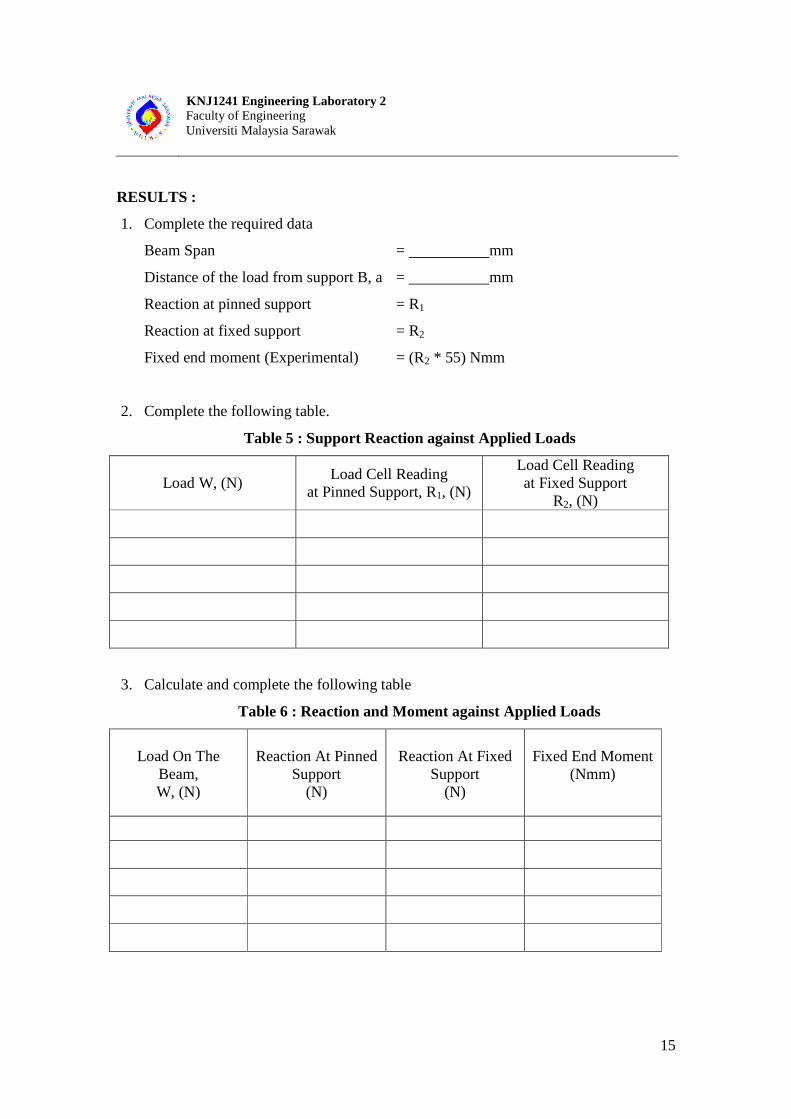
RESULTS :


Beam Span = mm

Distance of the load from support B, a = mm

Reaction at pinned support = R1

Reaction at fixed support = R2

Fixed end moment (Experimental) = (R2 * 55) Nmm

2. Complete the following table.

Table 5 : Support Reaction against Applied Loads

Load W, (N) Load Cell Reading

at Pinned Support, R1, (N)

Load Cell Reading at Fixed Support

R2, (N)

3. Calculate and complete the following table

Table 6 : Reaction and Moment against Applied Loads

Load On The

Beam, W, (N)

Reaction At Pinned

Support (N)

Reaction At Fixed

Support (N)

Fixed End Moment

(Nmm)


16

4. Using the data from the Table above plot the graph of:

(a) Fixed end moment verses load

(b) Reaction at the fixed support versus load

5. Determine the slope of each graph

6. Calculate the theoretical fixed end moment and reactions for 1 N load.

7. Determine the percentage error.

DISCUSSION :

1. For a beam loaded with a single point load as above, discuss the the relationship

between the fixed end moment and load as well as the reaction at the pinned support

and load.

2. Describe the change in the magnitude of the fixed end moment and the reaction at

the fixed support if the load moves away from the pinned support.

3. Compare and discuss the empirical and theoretical calculation.

4. List the possible cause of errors.


17

TITLE :

SD5 – Torsion of Shaft

THEORY :

Torsion is a straining action produced by couple moment that act normal to the axis of a

member. It is identified by a twisting deformation. When subjected only to torque, the

member is in pure torsion, which produces pure shear stresses. The shear properties of

materials are determined by a torsion test.

From the torsion theory the relationship between torque, section property, length,

material property, and angle of twist is given by,

T σ Gθ

J r L

Where T is the torque

r is the radius of the specimen where stress is to be determined

L is the length of the specimen

J is polar second moment of area of the section

G is the shear modulus of the material

σ is the stress at radius r

θ is the angle of twist in radian

From the above equation,

T Gθ

J L

Or

GJ

L

= =

=

T = x θ

(1)

(2)

(3)


18

Since G,J and L are constant for a particular experiment, therefore equation 3 can be

written as follows;

T = constant x θ

By plotting the graph of torque verses the angle of twist, the value of the constant can be

determined from the slope of the graph.

OBJECTIVE :

To determine the relationship between the applied torque and the angle of twist and hence

obtain the shear modulus.

APPARATUS :

Torsion apparatus, test specimen.


Beware of the apparatus controller; please don’t overdo the experiment to avoid the

failure of the specimen.

PROCEDURE :

1. Attach the specimen to the socket of the torsion apparatus. Measure the length and

diameter of the specimen.

2. Tighten all the parts including the protractor to read the degree rotation.

3. Apply torque to the specimen by pressing the motor switch to ‘test’ position.

Increase the load by 1N and for each increment switch off the motor to allow readings

to be taken. Whenever the motor is not capable of twisting the specimen further turn

the motor controller knob just slightly to increase the motor speed.

4. Record the load cell and the protractor readings for each load increment. The reading

of digital protractor can be omitted.

5. This experiment is to be conducted in the linear range only, it is advisable that the

torsional stress should not exceed 0.3 the yield stress of the material.

(4)


19

RESULTS :


Length of spesimen = mm

Diameter of spesimen = mm

Polar moment of inertia. = mm

Torque arm, L = mm

2. Record and calculate all the data in the following table

Table 7 : Experimental Data

Load Cell Applied Torque

Nmm Angle Of Twist

(degree) Angle of Twist

(radian)

3. Plot the graph of applied torque, T (Nmm) versus the angle of twist, θ (radian). Draw

the best fit curve through the plotted points.

4. Determine the slope of the graph. This represents the average torque per unit angle

of twist. Find the value of G.


20

DISCUSSION :

1. From the experimental data define the relationship between applied torque and angle

of twist.

2. How does the value of G obtained from the experiment compares with that normally

assumed in practice for the material being tested.

3. What are the possible sources of error in this experiment.

4. If the specimen is tested to failure describe the failure surface. Does it reflect the type

of material (brittle or ductile) being tested..


21

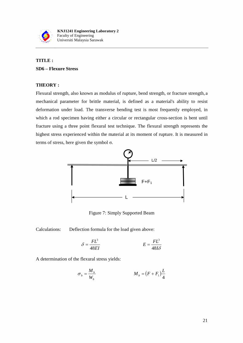
TITLE :

SD6 – Flexure Stress

THEORY :

Flexural strength, also known as modulus of rupture, bend strength, or fracture strength, a

mechanical parameter for brittle material, is defined as a material's ability to resist

deformation under load. The transverse bending test is most frequently employed, in

which a rod specimen having either a circular or rectangular cross-section is bent until

fracture using a three point flexural test technique. The flexural strength represents the

highest stress experienced within the material at its moment of rupture. It is measured in

terms of stress, here given the symbol σ.

Figure 7: Simply Supported Beam

Calculations: Deflection formula for the load given above:

δδ

I

FLE

EI

FL

4848

33

==

A determination of the flexural stress yields:

( )41

LFFM

W

Mb

b

bb +==σ

L

F+F1

L/2


22

When rectangular it is 12

3bhI = and

6

2bhWb =

When circular it is 64

4dI

π= and

32

3dWb

π=

δ = Deflection (mm.) E = Coefficient of Elasticity L = Span(mm.) I = Inertia Factor Mb = Moment of Flexure (Nmm) F1 = Load occasioned by weight of Load Device

(N) Wb = Resistance to Flexure (mm3) F = Load occasioned by additional weight (N) σb = Flexural Stress (N/mm2)

When E is calculated, the initial load caused by the load device has no significance since

the gauge has been set at zero with the device in place. However, when calculating

flexural stress, F1 is included.

OBJECTIVE :

To determine and compare the coefficient of elasticity for different materials.

APPARATUS :

Beam apparatus, beam specimen (steel, brass and aluminium), a set of weights.



tightened.

PROCEDURE :

1. Bolt the two supports to the support frame using the plate and bolt supplied with the

apparatus. The span is set at 500 mm and steel is employed

2. Mount load device and set the testing device.

3. Load with weights as shown in Table (shown in example) and read off the deflection.

(1 div = 0.01mm)

4. The test is repeated with test specimens of brass and aluminium.


23

RESULTS:


Beam Span, L = mm

Base length, b = mm

Height, h = mm

Weight load device, F1 = (N)

2. Complete the table with experimental results and calculate the coefficient of

Elasticity and the flexural stress.

Table 8 : Experimental Data

Material Load F (N)

Moment of Flexure

Mb (Nmm)

Flexural Stress

Deflection Coefficient of

Elasticity

σb

(N/mm2) δ

(mm) E

(N/mm2) Eave

(mm)

Steel

Brass

Aluminium

DISCUSSION :

1. Discuss the relationship between the Moment of flexure, Flexural Stress and

Coefficient of Elasticity with the increasing of loads.

2. Compare the Coefficient of Elasticity obtained with the theoretical value for each

material and discuss the results.


24


25

TITLE :

SD7 - Relation between Angular and Linear Speeds

THEORY :

Linear velocity is the distance travelled in a straight line per unit time while Angular

velocity is the angle travelled per unit time. Angular velocity expressed in the form of

what angle is rotated in a certain amount of time.

This relationship can be viewed in Uniform Circular Motion. For Instances, if ones

watches bicycle going along it is clear that, because there is no slippage between the

wheels and the road, there is a direct relationship connecting the linear speed along the

road and the rate at which the wheels turn. Instantaneously the speed at right angles to the

radius at the point of contact should be the rate of rotation of that radius.

OBJECTIVE :

To find the relationship between the angular rotation of a stopped shaft and the linear

travel of weights carried by cords wound round the shaft.

APPARATUS :

Mounting Bracket, Bob Weights, Measure Tape or Ruler.



tightened.


26

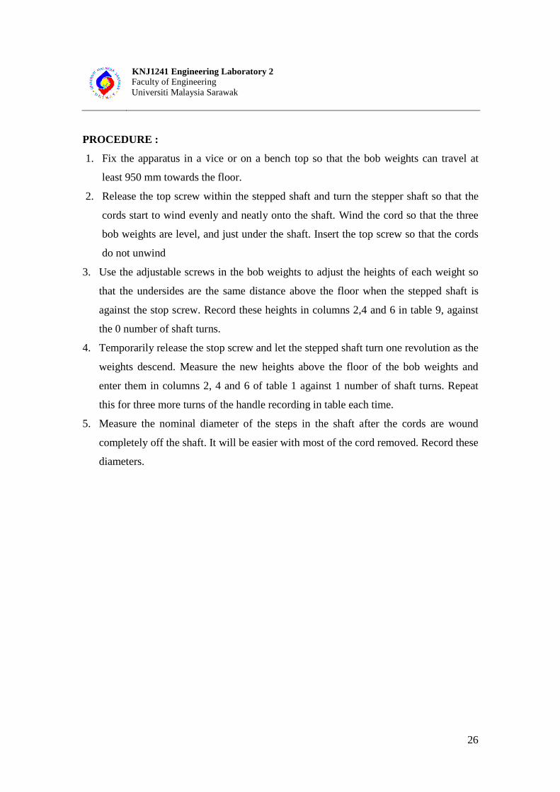
PROCEDURE :

1. Fix the apparatus in a vice or on a bench top so that the bob weights can travel at

least 950 mm towards the floor.

2. Release the top screw within the stepped shaft and turn the stepper shaft so that the

cords start to wind evenly and neatly onto the shaft. Wind the cord so that the three

bob weights are level, and just under the shaft. Insert the top screw so that the cords

do not unwind

3. Use the adjustable screws in the bob weights to adjust the heights of each weight so

that the undersides are the same distance above the floor when the stepped shaft is

against the stop screw. Record these heights in columns 2,4 and 6 in table 9, against

the 0 number of shaft turns.

4. Temporarily release the stop screw and let the stepped shaft turn one revolution as the

weights descend. Measure the new heights above the floor of the bob weights and

enter them in columns 2, 4 and 6 of table 1 against 1 number of shaft turns. Repeat

this for three more turns of the handle recording in table each time.

5. Measure the nominal diameter of the steps in the shaft after the cords are wound

completely off the shaft. It will be easier with most of the cord removed. Record these

diameters.


27

RESULTS :

1. Record all the required data in the following table.

Table 9 : Bob weight travel against shaft rotation for different diameters

1 2 3 4 5 6 7 Shaft Dia. Ø25 mm shaft Ø50 mm shaft Ø75 mm shaft

No. of turns of shaft, N

Height above floor (mm)

Distance Moved

s (mm)


Distance Moved

s (mm)


Distance Moved

s (mm)

0 1 2 3 4

2. Plot distance moved by each bob weight against turns of the shaft graph. Calculate

the gradient of each straight line and divide the gradients by the nominal diameters, d

to find the ratio in each case.

3. Convert the distances and rotation to linear and angular speeds by assuming that the

four turns of the shaft take four second.

DISCUSSION :

1. Comment on general accuracy of the results and suggest any improvements to the

procedure, which would minimize errors.

2. Describe was the relationship between the linear speeds and the angular rotation?

3. Why should the rpm of a drilling machine be varied to suit the size of the drill?


28


29

TITLE :

SD8 – Compound Pendulum

THEORY :

A compound pendulum, in its simplest form, consists of a rigid body suspended vertically

at a point which allows it to oscillate in small amplitude under the action of gravity.

Consider a bar suspended at point O and is free to oscillate.

Figure 8: A compound pendulum

O is the point of suspension

G is the centre of gravity

m is the mass of the body

θ is the angular displacement

α is the angular acceleration

I0 is the mass moment of inertia of the body

When the body is given a small displacement θ, the restoring moment about O to bring

the body back to its equilibrium position is given by:

Restoring moment, Mr = m×g×h sin θ (1)

Disturbing moment, Md = I0×α (2)


30

Since θ is small, sin θ = θ, therefore;

m×g×h = I0 ×α

α = (m×g×h) / I0 (3)

Periodic time = 2π × √(�� /�� )

= 2π × √(�/�)

= 2π × √(��/��ℎ) (4)

Frequency of motion, n = 1/ (periodic time) (5)

From parallel axis theorem,

I0 = Ig + mh2 (6)

Ig = m k2 (7)

Where k is the radius of gyration.

OBJECTIVE :

To determine the frequency of motion of a compound pendulum , mass moment of inertia

and the radius of gyration.

APPARATUS :

A simple compound pendulum (rod and a cylindrical bob weights), a stop watch.



tightened.


31

PROCEDURES :

A. Frequency of motion of the rod

1. If the bob weight is attached to the rod, remove it. Measure and record the diameter of

the rod.

2. Weigh and record the weight of the rod. Hang the rod at the point of suspension.

3. Hang the rod at the point of suspension. Measure and record the distance the point of

suspension from the end of the rod (close to the point of suspension) to obtain the

position of centre of gravity.

4. Displace the rod at a small angle and release the rod and start the stopwatch

simultaneously. Stop the watch after the rod has executed 5 cycles of oscillations.

Record this time in the Table provided.

5. Repeat step 5 for a few more times to get the average of time over 5 oscillations.

6. Remove the rod and hang it at a new point of suspension. Measure and record the

distance the point of suspension from the end of the rod (close to the point of

suspension).

7. Repeat step 3-6

B. Frequency of motion of the rod and bob weight

1. Take the bob weight and weight it. Record its weight

2. Measure and record the diameter of the bob weight to obtain the position of centre of

gravity.

3. Measure and record the thickness of the bob weight.

4. Decide the position of the bob weight on the rod and insert the rod through the hole in

the bob weight until the decided location. Tightened the screw on the bob weight against

the rod to hold the bob weight in position.

5. Measure the distance of the centre of gravity of the bob weight from the point of

suspension

6. Displace the rod at a small angle. Release the rod and start the stopwatch simultaneously.

7. Stop the watch after the rod has executed 5 cycles of oscillations.

8. Record the time in the Table provided.

9. Repeat step 6 to 8 for 10, 15 and 20 oscillations.

10. Repeat with a few more positions of the bob weight.


32

RESULTS :

1. Record the required data.

Part A:

Diameter of the rod = mm

Weight of the rod = mm

Length of the rod = mm

Part B:

Weight of the bob weight = mm

Diameter of bob weight = mm

Thickness of bob weight = mm

2. Tabulate the data in the following table.

Table 10 : Time of readings of time over 5 oscillations

Distance of the point of suspension from the top

end of the rod, mm

Time Taken, s

1 2 3 Average

3. Plot the data of average time taken against the distance.

4. Tabulate the following table.

Table 11 : Average time versus number of oscillations

Distance to the bob

weight (mm)

Number of Oscillations 5 10 15 20

1 2 3 �̅ 1 2 3 �̅ 1 2 3 �̅ 1 2 3 �̅


33

5. Plot the graph of average time (sec) versus number of oscillations (cycle)

6. Calculate the theoretical periodic time and hence the frequency of motion.

7. Calculate the mass moment of inertia about the point of suspension and radius of gyration

about axis passing through the centre of gravity.

DISCUSSION :

1. Describe your findings from the results obtained especially from the plotted graph.

2. Comment on general accuracy of the results and suggest any improvements to the

procedure, which would minimize errors.


34


35

TITLE :

SD9 – Flywheel Apparatus

THEORY :

Most machinery has parts, which revolve on their rotational axis; for example, wheels,

shafts, electric motors, centrifugal pumps, etc. This rotary motion is subject to the same

basic laws as linear motion, but all the terms have to be transformed to comply with the

special conditions of rotation.

For example the second law of motion changes as follows :-

Force = Mass × Acceleration ( F = ma)

Force × Radius = Rotational Mass × Rotational Acceleration

Couple = Moment of Inertia × Angular Acceleration (C=Iα)

The couple, C is also referred to as the torque, being the turning force exerted. The

application of this alternative form of the second law is widespread and most important in

understanding the performance of rotating machinery.

Where it is necessary to start rotating machinery quickly the moment of inertia must be as

small as possible to permit fast acceleration with the maximum value of torque.

On the other hand, when a reciprocating engine is required to run at a uniform speed

regardless of the fluctuation in driving force as each cylinder delivers power it is common

practice to increase the overall moment of inertia by adding a flywheel to the engine

shaft. A further use of flywheel is to store rotational energy, which is recoverable as it

slow down, thereby making a large couple available for a short period.

OBJECTIVE :

To determine the relationship between the angular acceleration of a flywheel and the

torque producing the acceleration.

APPARATUS :

Flywheel apparatus, bob weights, timer


36

SAFETY PRECAUTION :


tightened.

PROCEDURE :

1. Take the load hanger and pulling cord, and hook the end loop over the peg on the

flywheel shaft.

2. Wind up a definite number of turns; say 8, from the position where the cord falls off

the peg. This ensures that the driving torque due to a load on the hanger will act for a

set number of revolutions.

3. Wind up the pulling cord 8 turns and add a 10N load to the hanger. This load will

just allow the flywheel to rotate at a near constant angular velocity, and thus

overcome bearing function.

4. Hold the flywheel with one hand and a stopwatch in the other. The engraved mark

should be by the pointer at this stage.

5. Release the flywheel and start the watch. Count the revolutions with the aid of the

mark, using this to judge when to stop the watch as the set number of revolutions is

turned. The load hanger will fall onto the ground.

6. Repeat the above procedure adding load by increments of 1N. Keep on repeating the

experiment until at least six readings have been obtained. Try re-timing one or two

of the readings to see what the probable accuracy of the measurement is.


37

RESULTS :

1. Tabulate the times for the different values of mass plus hanger and calculate 1/t2

Table 12 : Acceleration of a Flywheel

No. of turns N

Weight mg (N)

Time (t) (s.)

1

�� Effective Couple

(Nm) 0 1 2 3 4 5 6 7 8

2. Plot the experimental results on a graph of total load against 1/t2, and draw the best

fit straight line through the points.

3. The gradient of the line provides an average value for the relationship between the

driving force and the angular acceleration, and should be multiplied by the

appropriate factor to obtain the value of k (that is, the moment of inertia). The

intercept on the total axis gives the initial load for which there is zero acceleration;

this must be the load required to overcome the friction in the bearings of the flywheel

shaft. Deduct this from the total load for each result and hence calculate the effective

couple, which should be entered in the table.

4. Convert the distances and rotation to linear and angular speeds by assuming that the

four turns of the shaft take four second.

DISCUSSION :

1. Compare the experimental and theoretical values of the moment of inertia obtained

in the experiment. Note the variability of any re-measured results of time, and of the

deduced friction if the experiment was repeated. Comment on the accuracy of the

experiment.

2. The theory, which was being verified, assumed the angular acceleration was uniform.

Can the experiment test this assumption?


38


39

TITLE :

SD10 – Belt Friction

THEORY :

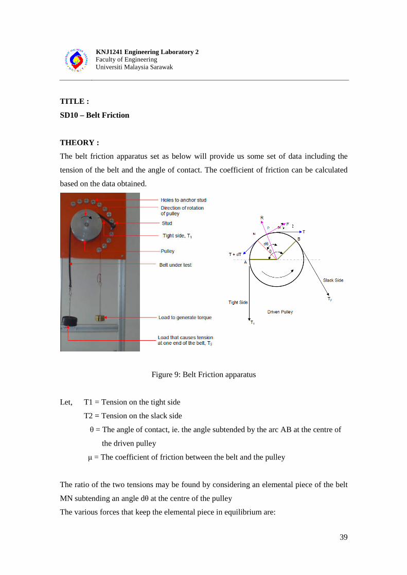
The belt friction apparatus set as below will provide us some set of data including the

tension of the belt and the angle of contact. The coefficient of friction can be calculated

based on the data obtained.

Figure 9: Belt Friction apparatus

Let, T1 = Tension on the tight side

T2 = Tension on the slack side

θ = The angle of contact, ie. the angle subtended by the arc AB at the centre of

the driven pulley

µ = The coefficient of friction between the belt and the pulley

The ratio of the two tensions may be found by considering an elemental piece of the belt

MN subtending an angle dθ at the centre of the pulley

The various forces that keep the elemental piece in equilibrium are:


40

(a) Tension T in the belt at M acting tangentially

(b) Tension T + dT in the belt at N acting tangentially

(c) Normal reaction R acting radially outward at P, where P is the mid point of

MN

(c) Friction force F = µR acting at right angle to R and in the opposite direction to

the motion of the pulley

The angle PCM = FMT = dθ/2

From the theory, we will obtain

R = T dθ (1)

R = dT / µ (2)

Equating (1) and (2) gives

T dθ = dT / µ

= µ dθ (3)

Intergrating Equation (3) gives

loge (T1 / T2) = µθ

or (T1 / T2) = eµθ (4)

The torque exerted on the driving pulley = (T1 – T2) * r1 (5)

For the this experiment T2 is the equal to the load applied at the hook end

T1 is obtained from equation (5)

By plotting the graph of loge (T1 / T2) versus θ the coefficient µ can be found.

OBJECTIVE :

To determine the coefficient of friction between belt and pulley

APPARATUS :

Belt friction apparatus, Set of Weights



tightened.


41

PROCEDURE :

1. Decide and record the angle θ.

2. Screw the stud to the mounting hole corresponding to this angle.

3. Hang a load hanger at the hook end of the belt.

4. Wound a cord round the pulley to apply torque to the system.

5. Hang a load hanger at the free end of the cord.

6. Apply tension to the belt by applying load on the hanger.

7. Place small weights on the torque hanger and observed the pulley. If the pulley does

not move, remove the load from the hanger. Increase the load and place it again on

the hanger. Repeat until the load on the hanger is able to rotate the pulley.

8. To get a more accurate result, adjust the last load on the hanger that causes the pulley

to rotate (decrease the load) and record the smallest load that causes the rotation.

This is the load that provides the torque just sufficient to overcome friction of the

belt.

9. Record the tension in the belt and repeat step 8 to 11 for a few more load increment.

10. Choose another angle θ and repeat the experiment.


42

RESULTS :

1. Record your observations for the load on belt and torque against angle.

Table 13 : Load on belt and torque hanger against angle

Stud Angle δ

Degrees

Angle of Contact, θ Degrees

Angle of Contact, θ Radian

Load on Belt, T2 (N)

Load on Torque Hanger, WT (N)

2. Plot the graph of T2 versus WT for each angle of contact.

3. Obtain the slope of each graph to obtain the average belt tension, T2 for each case.

4. Obtain the average values of T1 and T2 and fill the values in Table 2.

Table 14 : Average values of T1 and T2 against angle

Average T1 (N) Average T2 (N) Loge (T1/T2) Angle of Contact, θ, radian

5. Plot the graph of Loge (T1/T2) versus θ.

DISCUSSION :

1. Comment on the value of the coefficient of friction and the results.

2. How does the radius of the pulley affect the tensions in the belt?

3. How does the angle of contact affect the performance of the system?


43

APPENDIX A

SAFETY FIRST

• Follow all instructions carefully.

• Appropriate clothing must be worn in the lab. No loose clothing or jewelry around

operating equipment. Do not wear open toe shoes or sandal in operating laboratories.

• Do not operate equipment or carry on experiments unless the instructor/technician is

present in the laboratory.

• Assure that necessary safety equipment is readily available and in usable condition.

• Become familiar with safety precautions and emergency procedures before

undertaking any laboratory work.

• All injuries, no matter how small, must be reported.


44

APPENDIX B

GUIDELINES

• All laboratory works should be conducted within the period given.

• The laboratory rules and regulations apply throughout the lab sessions.

• Lab report should be submitted ONE (1) WEEK after every lab session.

• Attendance for every lab session is COMPULSORY. No mark will be given to any

report (s) submitted without attending the lab session (s).

• Reports must be written in the following format :-

� Formatting guidelines

– Font type & size : Times new roman, 12

– Spacing : 1.5 spacing

– Margin : left (1.5”), right (1.25”), top (1”) and

bottom (1”)

– Front Cover : Use Template Provided

– Tape binding

� Peers Evaluation Form – submit individually for every laboratory activity

weekly.

� Content guidelines

– Assessment Cover Page (only write the group name & signed by group’s

representative)

– Front Cover page

– Table of content

– Lab code & title of experiment

– Introduction / Theory

– Objectives

– Procedure

– Result

– Discussion

– Conclusion / recommendation

– References

cover - ENGINEERING LABORATORY AND...

Documents

Transcript of cover - ENGINEERING LABORATORY AND...